| Issue |
A&A
Volume 704, December 2025
|
|
|---|---|---|
| Article Number | A33 | |
| Number of page(s) | 12 | |
| Section | Interstellar and circumstellar matter | |
| DOI | https://doi.org/10.1051/0004-6361/202555641 | |
| Published online | 26 November 2025 | |
Edge-On Disk Study (EODS)
III. Molecular stratification in the Flying Saucer disk
1
Univ. Bordeaux, CNRS, Laboratoire d’Astrophysique de Bordeaux,
UMR 5804,
33600
Pessac,
France
2
Departamento de Física, Facultad de Ciencias, Universidad de Chile,
Av. Las Palmeras 3425,
Ñuñoa,
Santiago,
Chile
3
Dipartimento di Fisica e Astronomia, Università di Bologna,
via Gobetti 93/2,
40190
Bologna,
Italy
4
zAh/ITA, Heidelberg University,
Albert-Ueberle-Str. 2,
69120
Heidelberg,
Germany
5
Max-Planck-Institut für Astronomie (MPIA),
Königstuhl 17,
69117
Heidelberg,
Germany
6
IRAM,
300 Rue de la Piscine,
38046
Saint Martin d’Hères,
France
7
Institut des Sciences Moléculaires d’Orsay, CNRS, Univ. Paris-Saclay,
Orsay,
France
8
RIKEN Cluster for Pioneering Research,
2-1 Hirosawa,
Wako-shi,
Saitama
351-0198,
Japan
9
Carl Sagan Center, SETI Institute,
Mountain View,
CA,
USA
10
Aix-Marseille Univ, CNRS, CNES, LAM,
Marseille,
France
11
Konkoly Observatory, Research Centre for Astronomy and Earth Sciences,
Konkoly-Thege M. út 15-17,
1121
Budapest,
Hungary
12
Institute of Physics and Astronomy, ELTE Eötvös Loránd University,
Pázmány Péter sétány 1/A,
1117
Budapest,
Hungary
13
LUX, Observatoire de Paris, PSL Research University, CNRS, Sorbonne Universités,
92190
Meudon,
France
14
National Institute of Science Education and Research,
Jatni
752050,
Odisha,
India
15
Homi Bhabha National Institute,
Training School Complex, Anushaktinagar,
Mumbai
400094,
India
16
Astronomy Unit, School of Physics and Astronomy, Queen Mary University of London,
London
E1 4NS,
UK
17
National Astronomical Observatory of Japan, Division of Science,
2-21-1 Osawa, Mitaka,
Tokyo
181-8588,
Kanto,
Japan
18
Viet. Nat. Space Center, Viet. Academy of Science and Technology,
18, Hoang Quoc Viet, Nghia Do,
Cau Giay,
Ha Noi,
Vietnam
19
Academia Sinica Institute of Astronomy and Astrophysics,
No. 1, Sec. 4, Roosevelt Rd,
Taipei
106319,
Taiwan,
ROC
20
Institut für Theoretische Physik und Astrophysik, Christian-Albrechts-Universität zu Kiel,
Leibnizstraße 15,
24118
Kiel,
Germany
★ Corresponding author: This email address is being protected from spambots. You need JavaScript enabled to view it.
Received:
23
May
2025
Accepted:
29
September
2025
Abstract
Context. Investigating the vertical distribution of molecular content in protoplanetary disks remains difficult in most disks mildly inclined along the line of sight. In contrast, edge-on disks provide a direct (tomographic) view of the 2D molecular brightness.
Aims. We study the radial and vertical molecular distribution as well as the gas temperature and density by observing the Keplerian edge-on disk surrounding the Flying Saucer, a Class II object located in Ophiuchus.
Methods. We used new and archival ALMA data to perform a tomography of 12CO, 13CO, C18O, CN, HCN, CS, H2CO, c-C3H2, N2D+, DCN, and 13CS. We analyzed molecular tomographies and modeled data using the radiative transfer code DISKFIT.
Results. We directly measured the altitude above the mid-plane for each observed species. For the first time, we unambiguously demonstrate the presence of a common molecular layer and measure its thickness. Most molecules are located at the same altitude versus radius. Beyond CO, as predicted by chemical models, the CN emission traces the upper boundary of the molecular layer, whereas the deuterated species (DCN and N2D+) reside below one scale height. Our best fits from DISKFIT show that most observed transitions in the molecular layer are thermalized because their excitation temperature is the same, around ~17-20K.
Conclusions. These long-integration observations clearly reveal a molecular layer predominantly located around one to two scale heights at a temperature above the CO freeze-out temperature. The deuterated molecules are closer to the mid-plane, and N2D+ may be a good proxy for the CO snowline. Some molecules, such as CN and H2CO, are likely influenced by the disk environment, at least beyond the millimeter dust disk radius. The direct observation of the molecular stratification opens the door to detailed chemical modeling in a disk that appears representative of T Tauri disks.
Key words: astrochemistry / line: profiles / protoplanetary disks / ISM: abundances / radio lines: planetary systems / ISM: individual objects: Flying Saucer
© The Authors 2025
 Open Access article, published by EDP Sciences, under the terms of the Creative Commons Attribution License (https://creativecommons.org/licenses/by/4.0), which permits unrestricted use, distribution, and reproduction in any medium, provided the original work is properly cited.
This article is published in open access under the Subscribe to Open model. This email address is being protected from spambots. You need JavaScript enabled to view it. to support open access publication.
1 Introduction
Studying the gas and dust content of protoplanetary disks orbiting young low-mass stars is fundamental to unveiling the early phases of planet formation (Öberg et al. 2023). After low and moderate angular resolution studies revealed the inventory of the most abundant molecules (e.g., CO, HCO+, CN, HCN, CS, C2H, and H2CO) in T Tauri disks (e.g., Guilloteau et al. 2016b), the view of these gas-rich planet-forming disks has drastically improved thanks to the Atacama Large millimetre/submillimetre Array (ALMA). MAPS, the large program Molecules with ALMA at Planet-forming Scales (Öberg et al. 2021), studied the gas content of five large, relatively warm disks orbiting T Tauri and Herbig Ae stars, unveiling radial structures and allowing for more detailed analysis of chemistry (e.g., Guzmán et al. 2021; Öberg et al. 2023) and direct probing of the gas temperature (Law et al. 2021; Zhang et al. 2021).
The inclination of a disk with respect to the line of sight is an important parameter. Pole-on disks, such as that of TW Hya, allow detailed investigations of the gas and dust radial distribution (e.g., Teague et al. 2018; Andrews et al. 2012; Huang et al. 2018; Macías et al. 2021) but do not constrain the altitude at which the molecules reside inside the disk. For inclined disks, the situation is more favorable thanks to the Keplerian gradient (Dartois et al. 2003; Pinte et al. 2018), and their analysis provide very interesting results on the molecular chemistry (Bergin et al. 2016; Semenov et al. 2018; Guzmán et al. 2021; Kashyap et al. 2024). Recent papers using more sensitive ALMA observations and upgraded methods have improved our knowledge on the understanding of the stratification of the vertical molecular layer (e.g., Paneque-Carreño et al. 2022; Law et al. 2023; Paneque-Carreño et al. 2023; Hernández-Vera et al. 2024; Law et al. 2024; Paneque-Carreño et al. 2024; Keyte et al. 2024; Urbina et al. 2024; Temmink et al. 2025). Nevertheless, the accuracy obtained still strongly varies with radius because the intensity decreases with radius (>50-100 au) and the sensitivity becomes limited. While the altitude of the emitting layer can be estimated, this is not the case for the vertical width of the molecular layer, particularly for optically thin and moderate opacity lines, due to combined effects of inclination, density, temperature, and velocity gradients along the line of sight.
Edge-on disks, in contrast, are ideal targets to reconstruct the full 2D disk map by using its Keplerian rotation (Dutrey et al. 2017; Flores et al. 2021). We present new ALMA high angular resolution observations of the disk of the Flying Saucer (Grosso et al. 2003; Dutrey et al. 2017; Ruíz-Rodríguez et al. 2021), a Class II disk around a 0.60 M⊙ T Tauri star (Simon et al. 2019) located in Ophiuchus. An analysis of the continuum and CO data obtained in this project was presented in Guilloteau et al. (2025, hereafter Paper I). This second paper is dedicated to the first presentation of the extensive molecular dataset focused on the molecular stratification (based on 25 detected transitions) and contains an accompanying simple but robust analysis. Forthcoming papers will target molecules of specific interest.
2 Observations
2.1 Source presentation
The edge-on Flying Saucer disk, located in Ophiuchus at ~120 pc, was first imaged in the near-infrared domain by Grosso et al. (2003). The disk is not perfectly edge-on, and the scattered light morphology indicates that the southern part is closest to us (Grosso et al. 2003).
Using ALMA data from project 2013.1.00387.S at 0.5" resolution, Guilloteau et al. (2016a) reported that the dust disk is settled and close to edge-on (inclination >85°) and that it has an outer dust radius of ~180 au. They also measured the dust disk temperature because the emission of the bright CO background clouds is absorbed by the dust disk (~7 K). Dutrey et al. (2017) made the first CO and CS tomographies showing their vertical molecular extent in the Flying Saucer. Ruíz-Rodríguez et al. (2021) extended this to the analysis of CN emission available in the same dataset, revealing the relative stratification of CO, CN, and CS and estimating the excitation conditions in the outer region (~240 au) from the hyperfine intensity ratios of the N=2-1 transition.
The low dust and gas mid-plane temperature was confirmed by Guilloteau et al. (2025) (Paper I) using a higher angular data continuum and CO observations. Paper I also revealed the gas radial and vertical temperature gradients and how the surrounding CO clouds affect the CO emission.
2.2 Observations
In this work, we use the same ALMA Project 2023.1.00907.S (PI: O. Denis-Alpizar) as in Paper I. The project uses one spectral setup in Band 6 and another one in Band 7 and covers a large number of observed spectral lines (more than 20) at a spatial resolution as high as 0.18". Its spectral resolutions range from 0.040 to 0.2km s−1 (see Table A.1). We also included ALMA archival data from Projects 2013.1.00387 and 2013.2.00163.S that offer lower resolution observations of complementary spectral lines (Guilloteau et al. 2016a; Dutrey et al. 2017; Simon et al. 2019).
Observations and data reduction methods have already been presented in Paper I, and we summarize them in Appendix A.1. Imaging parameters are described in Appendix A.2.
3 Results from the tomographies and models
3.1 Tomographies
To present a synthetic view, we used the tomographic reconstruction method of Dutrey et al. (2017) that recovers the 2D molecular brightness temperature distribution using the velocity structure (Appendix A.3 presents the method). Figure 1 displays the tomographies that clearly reveal the vertical stratification of the molecular emission in the disk. In several cases there is little or no emission from the disk mid-plane. Figure 2 shows the superimposition of the 13CO tomography (in false color) with those of important molecules such as CN, HCN, CS, H2CO, DCN, and N2D+ (in black contours). The figure clearly reveals differences in the vertical location of the various molecular emissions. Making cuts through the tomographies illustrates this even better.
The vertical cuts in tomographies at various radii shown in Fig. A.1 reveal that the vertical emission profiles can be well approximated by two Gaussians, although some top and bottom differences are observed. These profiles were therefore fit by two Gaussians of the same width that were symmetrically placed below and above the disk plane for every radii. The intensities of the two Gaussians were kept as free parameters and then averaged, when needed.
The resulting fits with error bars are given in Fig. 3 and Figs. A.2–A.4. Fig. 3 shows the altitude and (deconvolved) thickness of the molecular emission. Fig. A.2 shows the radial extent and intensity. Fig. A.3 presents the south-to-north ratio that is discussed in Sect. 4.1. The measured widths (Fig. A.4) were deconvolved from the appropriate beam size for each line (bottom part of Fig. 3). Comparisons of Fig. A.4 with the bottom part of Fig. 3 show that the beam impact is small, except for the low-resolution (0.5") data where deconvolved widths are in agreement with those obtained at higher resolution. This clearly confirms that the thickness of the molecular layer is measured.
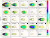 |
Fig. 1 Tomographic view of the observed spectral lines showing the mean brightness as a function of radius and height (both in au). Original beam sizes are indicated in the upper-right corner of each panel. CN hyperfine transitions are labeled by their frequency in MHz. Contour levels are 0.5-2 by 0.5, 3-10 by 1, and 12-30 by 2 K (except for the weak para-H2CO line, contour, at 0.25 K only). The panel labeled “CN Singles” shows a weighted average of three unblended lines at 338 516, 340 008, and 340 019 MHz, which is shown with a contour step of 0.25 K. The continuum at 230 GHz is shown in the bottom-left panel with contour levels 0.1, 0.2, 0.4, 0.8, and 1.2 K. |
3.2 Disk model fitting
While the tomography unveils the geometry, it is not capable of recovering the intrinsic physical parameters, such as molecular column densities. To do so, we used the parametric radiative transfer code DISKFIT (Piétu et al. 2007). Table 1 presents the best-fit model for each molecule (apart from CN, where the hyperfine structure allowed for fitting of the 3-2 and 2-1 transitions separately).
The analysis with DISKFIT is intended to provide the main properties of the 30-200 au region of the disk (where the dust disk extends), particularly the excitation temperature of the observed transitions and molecular surface densities. For this purpose, we adopted a simple Keplerian disk model with power law radial distributions and sharp edges. All radial quantities (temperatures, surface densities, scale heights) are power laws in the form x(r) = x0(r/r0)−ex, with ro being the reference radius taken to be 100 au. The local line width, δV, was assumed constant because of limited signal to noise. The model also incorporates continuum emission from dust, using the best-fit model from Paper i.
The molecular level populations are described by rotation temperatures that only depend on radius. The vertical molecular density profile is a Gaussian of independent (fit) scale height:

Each molecule, m, therefore has a different apparent scale height, Hm (r), that characterizes the vertical location of the bulk emission of the given molecule. in addition, to represent the lack of emission near the mid-plane, molecules are absent at all heights where z < ZdHm(r). For simplicity, here we assumed that Zd does not depend on r. A graphic representation of the temperature and density distributions for key molecules is given in Fig. 4. These approximations do not allow proper representation of the outer regions (r > 250 au, where the emission reaches the midplane) but are appropriate for the bulk of emission (see Fig. 1).
The apparent scale height and depletion level, Zd, are derived to reproduce the vertical brightness distribution, including the effect of line opacity. For Zd ~ 0.6, most molecules reside around Hm (r), which is thus comparable to the apparent height of the molecular layer seen in Fig. 3. An exception is CO, because of the large opacity of the 2-1 transition but also the increase in temperature in the disk atmosphere. The molecule dependent scale heights, Hm , should not be confused with the hydrostatic scale height of gas distribution, and Fig. 4 shows that the latter is about a factor of two smaller than those of CN, HCN, or CS.
For DCN and N2D+, which are located around the midplane in Fig. 1 (and thus required Zd ~ 0), assuming a scale height of 11 au (in agreement with the mid-plane temperature of 10 K) does not change the derived surface density within the current noise level. However, the vertical spread of DCN is best represented with an H(r) similar to that of the other molecules.
For the temperature, we used the local thermodynamic equilibrium (LTE) approximation, in which the molecular level population is controlled by a single temperature (see Piétu et al. 2007, for the interpretation of this temperature). DISKFIT then solved the radiative transfer equation along any line of sight by ray tracing while accounting for velocity gradients and the hyperfine structure of the spectral lines. Comparison to the data was made by comparing the interferometric visibilities resulting from the modeled intensity distribution to the observations.
The minimization was done through a Levenberg-Marquardt scheme, with multiple restarts (about ten) to avoid secondary minima. Error bars were taken from the covariance matrix. The disk orientation, inclination, and rotation velocity were derived from all strong lines, yielding consistent results (Table B.1). The kinematics was checked and found to be Keplerian for all lines. Line frequencies were taken from the Cologne database for molecular spectroscopy (CDMS). Details about individual molecules are given in Appendix B.
Apart from CO, the molecules are vertically concentrated around a relatively narrow altitude range. Fig. 4 shows that the best model assuming a vertical temperature gradient (Paper i) samples temperatures from 15 to 20 K in this altitude range. Our independently fit isothermal values fall exactly in this range and are thus representative of the average temperature of the molecular layer. Moreover, this isothermal assumption does not significantly affect the derived surface densities because in the relevant temperature range (15-20 K), the brightness of the observed transitions in the optically thin regime only depends weakly on temperature (see Fig. 4 of Dartois et al. 2003). Figure 5 shows the tomography of the residuals for lines with a signal-to-noise ratio high enough.
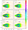 |
Fig. 2 13 CO tomography in false color with superimposition of the tomographies (black contours) of HCN 4-3, CS 7-6, and CN at 340.348 GHz; p-H2CO at 218.222 GHz; and DCN 3-2 and N2D+ 3-2. Contours are in steps of 1.5 K for HCN, CS, CN, and p-H2CO; 0.75 K for DCN; and 0.375 K for N2D+. The gray ellipses indicate the impact of line width on the effective beam at 80 and 240 au |
4 Discussion
4.1 Vertical molecular stratification
Molecular layer. Figures 1 and 3 reveal that, with the exception of 12CO and the deuterated species, all molecules reside in a well-defined layer at an altitude scaling linearly with radius up to about 200 au. The spatial resolution biases this altitude below −70 au because the two disk sides are no longer sufficiently separated (this bias is much larger for CS 5-4 or ortho-H2CO at 211.211 GHz due to their lower 0.5-0.6" resolution). Figs. 2 and 3 clearly show that the CN emission is more extended than those of HCN and CS, the latter being closer to the mid-plane. On the contrary, the DCN and N2D+ emissions clearly appear around the mid-plane.
The existence of such a well defined molecular layer has been predicted by many models over the last 20 years (e.g., Aikawa et al. 2002); see also Dutrey et al. (2014); Öberg et al. (2023) for reviews). The edge-on geometry provides for the first time the opportunity to directly measure the geometrical thickness of the molecular layer, as demonstrated in Fig. 3 (see also Appendix A.3 and Fig. A.4). We find that the deconvolved layer thickness also scales approximately linearly with the radius.
The DISKFIT results (Table 1) show that part of the disk mid-plane is devoid of molecules such as CN, CS, HCN, H2CO, 13CO, and C18O. The apparent scale heights of the molecular distributions at 100 au (Hm, Col.4) are all similar (18-20 au), and there is no molecular emission below the altitude zd(r) ≈ 0.5H(r) for the molecules (including 13CO) except the deuterated species and c-C3H2. Finally, CS and 13CS are located at the same altitude.
This is the first clear demonstration of a physical molecular layer that is common to many molecules. The width of the molecular layer is also properly measured thanks to the edge-on inclination, with molecular vertical freeze-out likely happening over a few au. For comparison, Paneque-Carreño et al. (2023) reported in their sample of seven inclined TTauri and Herbig Ae disks a molecular layer located at z/r ≤ 0.15 (see their Figs. 9 and 10). In our case, we clearly find z/r ≃ 0.2 inside a radius of 200 au and z/r ≃ 0.15-0.2 beyond for all molecules with the exception of CO, which is at a higher z/r ≃ 0.3, and the deuterated species, which are at z/r ≃ 0.1-0.12.
Molecules near the mid-plane. The emission from N2D+, DCN, and c-C3H2 is located closer to the mid-plane (Figs. 2 and 3), with the best fits converging toward Zd = 0. Following Willacy (2007), DCN is formed around ~10K via ion-molecule reactions. We therefore assumed a temperature of 10 K to derive the column density, checking that this value (consistent with the mid-plane temperature found in Paper I) does not affect the other parameters, in particular Zd. We only found a difference in surface density, Σ, of 30%.
Majumdar et al. (2017) and Aikawa et al. (2018) found that the formation of N2D+ is very efficient at low temperatures when CO is frozen onto grains, and it then becomes enhanced in the cold mid-plane. Thus N2D+ may trace the CO snow line better than N2H+. Cataldi et al. (2021) reported that the inner radius of the N2D+ column density profile roughly corresponds to the location of the CO snowline in most sources of project MAPS (except GM Aur because of a low S/N ratio). In the Flying Saucer, despite a limited S/N ratio, the N2D+ emission coincides with the location of the hole observed in CO (Figs. 1 and 2) at radius ~ 200 au.
South-to-north asymmetry. In a flared disk not exactly edge-on, the nearest side will be seen at a higher inclination angle that the most distant side. For partially optically thick lines, the outer (colder) regions will self-absorb the emission coming from the innermost (warmer) zones. In contrast, the furthest side is seen more face on, allowing the warmer regions to be directly seen. Hence, the furthest side should appear warmer. This was mentioned for the first time by Guilloteau & Dutrey (1998) for data in DM Tau, and it has since been used in many disks to recover the full disk orientation. The specific case of edge-on disks not exactly at 90 degrees is modeled in Dutrey et al. (2017).
A south-to-north asymmetry is exhibited by CO, CS, and the inner region in HCN (Fig. A.3), which is consistent with the known disk orientation with a brighter northern side. However, for molecules with low or moderate opacity, the southern side appears brighter, at least beyond the dust disk radius in the 150-200 to 300 au range. This is more pronounced at the lowest opacities (C18O, H2CO) than for CN (and HCN in the outer part). There is no obvious explanation for this intrinsic asymmetry. It may result from a difference in the disk illumination caused, for example, by an unseen disk warp or by an asymmetry in the external UV field. In this respect, Dutrey et al. (2017) noted that the Flying Saucer is located on the eastern side of the ρ Oph cloud, while most B stars are located on the western side, thus allowing dense clouds to absorb most of their UV radiation.
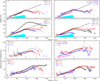 |
Fig. 3 Top: altitude A(r) of the molecular layer as a function of radius. The black curve is the HCN(4-3) altitude for comparison. The cyan region indicates the approximate size of the dust disk. The dotted line corresponds to z/r = 0.2. Bottom: deconvolved thickness of the molecular layer. The deconvolution has been done assuming Gaussian shapes using the clean beam minor axis since synthesized beams are elongated almost parallel to the disk plane. The black curve is the HCN(4-3) thickness, for comparison. The cyan bar marks the edge of the dust disk. |
Model fitting results.
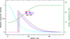 |
Fig. 4 Profiles resulting from DISKFIT at 100 au. The green curve is the temperature profile, and the cyan curves indicate the H2 density structure (thin: under isothermal assumption at the mid-plane temperature (10 K); thick: using the full temperature profile) that were derived from the CO analysis by Guilloteau et al. (2025). The other colored curves are the molecular density profiles for CS (red), HCN (black), CN 2-1 (blue), and 3-2 (magenta) and are based on the parameters from Table 1. The corresponding horizontal bars indicate the measured temperatures and the density weighted average height of the emission. |
4.2 Radial distribution
The radial distribution can be roughly separated in four parts: an inner cavity, a first molecular ring, a large gap (in the mid-plane), and a second molecular ring (or second emission peak) located beyond the millimeter dust outer radius. The sizes of the cavities and gaps vary depending on the molecules, and the second molecular ring is not always seen.
Inner radii. Dutrey et al. (2017) reported an upper limit on a possible central hole of ~15 au for CO and ~25 au for CS based on the position-velocity diagrams. This is roughly consistent with the values we determined for the CO and CS lines using DISKFIT. The continuum does not exhibit a central cavity and is not optically thick enough to hide molecules with an average dust opacity of ~0.2 (Paper I). Moreover, the size of the central cavity is slightly larger for CN (~50 au), suggesting that chemical effects may play a role in creating these inner depressions.
The H2CO and N2D+ emissions exhibit very large inner cavities (Table 1 and Fig. A.2). H2CO emission extends from radii of 130 au to 300 au, i.e., most of the H2CO emission comes from beyond the dust disk. N2D+ emission has an inner radius of 80 au, and its maximum intensity is near the dust disk outer radius (~ 200 au), where there is a very large gap in the CO emission. This large gap is also clearly seen in Fig. 2.
Rings in the molecular layer. In the molecular layer, the radial distribution of CO emission cannot be simply interpreted due to confusion with the surrounding clouds (see Paper I for details). However, the 13CO and C18O emissions, which are essentially free of confusion, peak exactly in the same radius range, 150-180 au.
In contrast, the maximum intensity of the optically thin 13 CS 5-4 emission radially coincides with the radial location of the maximum intensity of the CS 7-6 emission (~120 au, Fig. A.2). The CN 3-2 and HCN 4-3 emission also peaks at a radius of ~ 120 au, similar to CS. The DCN emission is prominent at radii of 70-100 au and then 200-220 au. This suggests the existence of at least two resolved rings (see also Fig. A.2), as already observed in less inclined disks (e.g., Öberg et al. 2023). Cataldi et al. (2021) also reported the presence of DCN beyond the radius of the millimeter dust disk in IM Lupi and GMAur. The c-C3H2 emission peaks at 70-80 au, similar to the first peak of the DCN emission. Unlike other species, the H2CO emission exhibits two maxima located beyond a radius of 150 au. The outer radius of the continuum is at ~ 180 au, and most of the H2CO emission extends outside of the dust disk.
In conclusion, with the exception of CO lines, there are at least two bright molecular areas. One is in an inner region extending from about 50 to 150 au, and the second is in an outer ring (secondary emission peak) peaking beyond the millimeter dust outer radius at 200-220 au (see also Fig. 2).
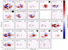 |
Fig. 5 Tomographies of the residuals of the DISKFIT models. For each line, the best-fit model visibilities are subtracted from the observed ones and imaged as done for observations. The tomographic method is then applied on these residual data cubes. Contour spacings are 0.5 K. |
4.3 Temperature in the molecular layer
Table 1 shows that the temperature in the molecular layer is about 17-20 K. 13 CO is partially optically thick and provides a temperature measurement in the radius range 150-200 au. Our vertically isothermal analysis provides results in excellent agreement with those obtained in Paper I with a temperature model that follows the vertical prescription by Dutrey et al. (2017). This justifies our simplified assumption with only 12CO probing the uppermost layers. This is also clearly demonstrated by Fig. 4, which compares the average temperature derived from this paper with the temperature derived from CO using the more physical description of Paper i.
The derived temperature is always slightly above the CO freeze-out temperature of 17 K (Qi et al. 2013, although there are variations on the exact value for the CO freeze-out temperature, e.g., Qi et al. 2019). Nevertheless, the derived temperature can be considered as representative of the gas temperature in the bulk of the molecular layer. Similarly, Foucher et al. (2025) reported, for the molecular layer of the cold edge-on disk of SST-Tau 042021, a temperature (derived from CO and 13 CO ALMA data) that is also almost radially constant and also slightly above the CO freeze-out temperature of 17 K.
Radial dependence. The temperature also appears almost constant in the radius range 50-200 au. The value of exponent q is close to zero for the CS, HCN, and CO isotopologues. Our dual line analysis (J=5-4 and J=7-6) of CS yielded a temperature that is in excellent agreement with that found by Dutrey et al. (2017) based only on the transition of 5-4.
The case of CN. For CN, we were able to measure the temperature independently for each transition thanks to the hyperfine structure that directly constrains the line opacities (see Appendix B for details). The same value of 19-20 K was found for the N=2-1 and N=3-2 transitions. Ruíz-Rodríguez et al. (2021) used the same CN 2-1 data at a 0.5" resolution to derive the temperature in the outer disk, beyond 210 au, and found T ≈ 12 K in the mid-plane. Although our model is based on measurements at smaller radii, our extrapolated value at 250 au is ~13 K.
4.4 Surface density in the molecular layer
The CO isotopologues show flat surface density profiles (p ≃ 0). The 13CO/C18O ratio of approximately eight, which is consistent with the local elemental isotopic ratios (Wilson & Rood 1994), suggests a relatively limited impact of selective photo-dissociation and fractionation in the molecular layer for CO (Langer et al. 1980; Miotello et al. 2014). The derived CS/13CS ratio of about 50 also excludes strong fractionation in this molecule (Wilson & Rood 1994; Rodríguez-Baras et al. 2021).
The HCN, CS, and c-C3H2 lines exhibit a steep decline with radius (exponent p). This may be due in part to excitation conditions, at least for CS and HCN. The surface densities of CN and H2CO have an intermediate behavior (p ~ 1.5) since their emission extends beyond the radius of the dust disk. This may be related to significant changes in chemistry and illumination. The CN surface density, ~1.2 ∙ 1014cm−2 at radius 100 au, and the CN/HCN ratio (~10) are also similar to the values quoted by Bergner et al. (2021) in IM Lupi and GM Aur.
Finally, we compared the results from Table 1 with the surface densities derived from 30 T Tauri disks by Guilloteau et al. (2016a). This comparison clearly shows that the Flying Saucer disk exhibits gas properties representative of those of T Tauri disks.
4.5 Departure from a simple model
Figure 5 shows the tomographies of the residual emission after subtraction of our best-fit DISKFIT model from the data. The CO emission cannot be discussed in a simple manner due to the confusion of the CO cloud. 13CO is also affected to some extent, which may partially explain its anomalous south-north intensity ratio. However, other molecules are free of confusion. Beyond 200 au, CN, HCN, CS, and to a lesser extent 13CO clearly exhibit emission close to the disk mid-plane from the outer ring. As our disk model assumes the emission height varies as a power law, it is unable to properly represent the regions beyond about 200 au, where the altitude of the molecular layer starts decreasing (see Fig. 3).
These residuals also reveal that CN appears more extended vertically than in our simple model, with significant residuals above the common molecular layer. Such residuals are much fainter in HCN, although fit results in Table 1 do not indicate significant differences in the altitude of CN and HCN. This indicates that CN, although predominantly located in the molecular layer, extends to higher altitudes, as expected because of its sensitivity to UV radiation. A more complex approach is needed to quantify this behavior. CS displays an intermediate behavior between CN and HCN in this respect. The H2CO location is also different than our simple assumption, being more extended both vertically and radially. These residuals indicate that our assumed vertical profiles, displayed in Fig. 4, may require a more pronounced tail at high altitudes instead of our assumed Gaussian drop-off.
5 Conclusion and perspectives
For the first time, we clearly show that most molecules (apart from the deuterated species) reside in a common molecular layer, and we were able to measure its geometrical thickness. Furthermore, the transition between the depleted mid-plane and the lower edge of this layer seems to occur over a few au (see Fig. 4). This unique dataset provides new insights that deserve more sophisticated thermo-chemical modeling in order to be understood, as illustrated by Figs. 1 and 5. We emphasize some important points here.
We find that the molecular layer is at z/ r ~ 0.2, which is larger than in the sample studied by Paneque-Carreño et al. (2023) (z/r ≤ 0.15). This difference is perhaps due to the lower disk temperature, as the central star is of lower mass than in their sample. This needs to be confirmed by studying other edge-on disks;
The molecular layer has a relatively shallow radial temperature profile, ~17-20 K at radius 100 au, only slightly above the CO freeze-out temperature;
As predicted by astrochemical models (e.g., Aikawa et al. 2018), the deuterated species are clearly located closer to the mid-plane, but they are likely at a lower altitude than estimated for TW Hydra (Romero-Mirza et al. 2023). N2D+ emission has a low S/N ratio, but its extent suggests that N2D+ may be a good tracer of the CO snowline. Comparing N2H+ and N2D+ distributions would be invaluable;
As visible from Figs. 5 and A.1, although CN has a scale height similar to the other molecules, the CN layer appears slightly more vertically extended than most of the other molecules except for CO (see also Paneque-Carreño et al. 2022), probably because of its sensitivity to UV radiation (Cazzoletti et al. 2018; Nomura et al. 2021; Ruaud 2021). Yoshida et al. (2024) and Paneque-Carreño et al. (2023) observed the same behavior in the case of TW Hydra and Elias 2-27, respectively. For Elias 2-27, the behavior appears compatible with predictions from thermo-chemical models. Large CN radial extents (in part beyond millimeter dust disks) have also been seen by Bergner et al. (2021) for the five sources of the MAPS project;
The H2CO distribution has a large central cavity and peaks beyond the dust disk edge, a situation similar to that found by Guzmán et al. (2021); Hernández-Vera et al. (2024) for AS 209, HD 163296, and IM Lupi. The ortho-para ratio is around two and consistent with the low temperature of 1214 K. The different slopes (p) indicate that this ratio may increase with radius. This may reflect the formation of H2CO by two different routes: a cold formation path on grain surfaces (Fayolle et al. 2016) and a gas-phase path, such as for DM Tau (Loomis et al. 2015);
The c-C3H2 emission steeply decreases with radius, such as for 13CS, but appears somewhat below the molecular layer. The latter point is also reported by Paneque-Carreño et al. (2023) in the case of the warmer disk of HD 163296;
Finally, several molecular emissions have a secondary emission peak or outer ring beyond the millimeter dust outer radius, suggesting that photo-desorption may play an important role for many molecules to replenish the gas phase in cold disks around T Tauri stars.
These points clearly deserve deeper observational and model studies to confirm the observed behaviors on more sources in different molecules.
Acknowledgements
This work was supported by the Thematic Actions PNPS and PCMI of INSU Programme National “Astro”, with contributions from CNRS Physique & CNRS Chimie, CEA, and CNES. N.T.P. acknowledges support from the Vietnam Academy of Science and Technology under grand number VAST 08.02/25-26. Y.W.T. acknowledges support through NSTC grant 111-2112-M-001-064- and 112-2112-M-001-066-. This work was also supported by the NKFIH NKKP grant ADVANCED 149943 and the NKFIH excellence grant TKP2021-NKTA-64. This paper makes use of the following ALMA data: ADS/JAO.ALMA#2013.1.00163.S, ADS/JAO.ALMA#2013.1.00387.S and ADS/JAO.ALMA#2023.1.00907.S. ALMA is a partnership of ESO (representing its member states), NSF (USA) and NINS (Japan), together with NRC (Canada), NSTC and ASIAA (Taiwan), and KASI (Republic of Korea), in cooperation with the Republic of Chile. The Joint ALMA Observatory is operated by ESO, AUI/NRAO and NAOJ.
References
- Aikawa, Y., van Zadelhoff, G. J., van Dishoeck, E. F., & Herbst, E. 2002, A&A, 386, 622 [NASA ADS] [CrossRef] [EDP Sciences] [Google Scholar]
- Aikawa, Y., Furuya, K., Hincelin, U., & Herbst, E. 2018, ApJ, 855, 119 [NASA ADS] [CrossRef] [Google Scholar]
- Andrews, S. M., Wilner, D. J., Hughes, A. M., et al. 2012, ApJ, 744, 162 [NASA ADS] [CrossRef] [Google Scholar]
- Bergin, E. A., Du, F., Cleeves, L. I., et al. 2016, ApJ, 831, 101 [Google Scholar]
- Bergner, J. B., Öberg, K. I., Guzmán, V. V., et al. 2021, ApJS, 257, 11 [NASA ADS] [CrossRef] [Google Scholar]
- Cataldi, G., Yamato, Y., Aikawa, Y., et al. 2021, ApJS, 257, 10 [NASA ADS] [CrossRef] [Google Scholar]
- Cazzoletti, P., van Dishoeck, E. F., Visser, R., Facchini, S., & Bruderer, S. 2018, A&A, 609, A93 [NASA ADS] [CrossRef] [EDP Sciences] [Google Scholar]
- Dartois, E., Dutrey, A., & Guilloteau, S. 2003, A&A, 399, 773 [CrossRef] [EDP Sciences] [Google Scholar]
- Dutrey, A., Semenov, D., Chapillon, E., et al. 2014, in Protostars and Planets VI, eds. H. Beuther, R. S. Klessen, C. P. Dullemond, & T. Henning, 317 [Google Scholar]
- Dutrey, A., Guilloteau, S., Piétu, V., et al. 2017, A&A, 607, A130 [CrossRef] [EDP Sciences] [Google Scholar]
- Fayolle, E. C., Balfe, J., Loomis, R., et al. 2016, ApJ, 816, L28 [Google Scholar]
- Flores, C., Duchêne, G., Wolff, S., et al. 2021, AJ, 161, 239 [NASA ADS] [CrossRef] [Google Scholar]
- Foucher, C., Dutrey, A., Piétu, V., et al. 2025, A&A, 704, A32 [NASA ADS] [CrossRef] [EDP Sciences] [Google Scholar]
- Grosso, N., Alves, J., Wood, K., et al. 2003, ApJ, 586, 296 [Google Scholar]
- Guilloteau, S., & Dutrey, A. 1998, A&A, 339, 467 [Google Scholar]
- Guilloteau, S., Piétu, V., Chapillon, E., et al. 2016a, A&A, 586, L1 [NASA ADS] [CrossRef] [EDP Sciences] [Google Scholar]
- Guilloteau, S., Reboussin, L., Dutrey, A., et al. 2016b, A&A, 592, A124 [NASA ADS] [CrossRef] [EDP Sciences] [Google Scholar]
- Guilloteau, S., Denis-Alpizar, O., Dutrey, A., et al. 2025, A&A, 700, L5 [NASA ADS] [CrossRef] [EDP Sciences] [Google Scholar]
- Guzmán, V. V., Bergner, J. B., Law, C. J., et al. 2021, ApJS, 257, 6 [CrossRef] [Google Scholar]
- Hernández-Vera, C., Guzmán, V. V., Artur de la Villarmois, E., et al. 2024, ApJ, 967, 68 [CrossRef] [Google Scholar]
- Huang, J., Andrews, S. M., Cleeves, L. I., et al. 2018, ApJ, 852, 122 [Google Scholar]
- Kashyap, P., Majumdar, L., Dutrey, A., et al. 2024, ApJ, 976, 258 [Google Scholar]
- Keyte, L., Kama, M., Booth, A. S., Law, C. J., & Leemker, M. 2024, MNRAS, 534, 3576 [Google Scholar]
- Langer, W. D., Goldsmith, P. F., Carlson, E. R., & Wilson, R. W. 1980, ApJ, 235, L39 [NASA ADS] [CrossRef] [Google Scholar]
- Law, C. J., Teague, R., Loomis, R. A., et al. 2021, ApJS, 257, 4 [NASA ADS] [CrossRef] [Google Scholar]
- Law, C. J., Booth, A. S., & Öberg, K. I. 2023, ApJ, 952, L19 [NASA ADS] [CrossRef] [Google Scholar]
- Law, C. J., Benisty, M., Facchini, S., et al. 2024, ApJ, 964, 190 [NASA ADS] [CrossRef] [Google Scholar]
- Loomis, R. A., Cleeves, L. I., Öberg, K. I., Guzman, V. V., & Andrews, S. M. 2015, ApJ, 809, L25 [Google Scholar]
- Macías, E., Guerra-Alvarado, O., Carrasco-González, C., et al. 2021, A&A, 648, A33 [EDP Sciences] [Google Scholar]
- Majumdar, L., Gratier, P., Ruaud, M., et al. 2017, MNRAS, 466, 4470 [Google Scholar]
- Miotello, A., Bruderer, S., & van Dishoeck, E. F. 2014, A&A, 572, A96 [NASA ADS] [CrossRef] [EDP Sciences] [Google Scholar]
- Nomura, H., Tsukagoshi, T., Kawabe, R., et al. 2021, ApJ, 914, 113 [NASA ADS] [CrossRef] [Google Scholar]
- Öberg, K. I., Guzmán, V. V., Walsh, C., et al. 2021, ApJS, 257, 1 [CrossRef] [Google Scholar]
- Öberg, K. I., Facchini, S., & Anderson, D. E. 2023, ARA&A, 61, 287 [CrossRef] [Google Scholar]
- Paneque-Carreño, T., Miotello, A., van Dishoeck, E. F., et al. 2022, A&A, 666, A168 [NASA ADS] [CrossRef] [EDP Sciences] [Google Scholar]
- Paneque-Carreño, T., Miotello, A., van Dishoeck, E. F., et al. 2023, A&A, 669, A126 [NASA ADS] [CrossRef] [EDP Sciences] [Google Scholar]
- Paneque-Carreño, T., Izquierdo, A. F., Teague, R., et al. 2024, A&A, 684, A174 [NASA ADS] [CrossRef] [EDP Sciences] [Google Scholar]
- Park, I. H., Wakelam, V., & Herbst, E. 2006, A&A, 449, 631 [NASA ADS] [CrossRef] [EDP Sciences] [Google Scholar]
- Piétu, V., Dutrey, A., & Guilloteau, S. 2007, A&A, 467, 163 [Google Scholar]
- Pinte, C., Ménard, F., Duchêne, G., et al. 2018, A&A, 609, A47 [NASA ADS] [CrossRef] [EDP Sciences] [Google Scholar]
- Qi, C., Öberg, K. I., Wilner, D. J., et al. 2013, Science, 341, 630 [Google Scholar]
- Qi, C., Öberg, K. I., Espaillat, C. C., et al. 2019, ApJ, 882, 160 [Google Scholar]
- Rodríguez-Baras, M., Fuente, A., Riviére-Marichalar, P., et al. 2021, A&A, 648, A120 [NASA ADS] [CrossRef] [EDP Sciences] [Google Scholar]
- Romero-Mirza, C. E., Öberg, K. I., Law, C. J., et al. 2023, ApJ, 943, 35 [CrossRef] [Google Scholar]
- Ruaud, M. 2021, ApJ, 916, 103 [CrossRef] [Google Scholar]
- Ruíz-Rodríguez, D., Kastner, J., Hily-Blant, P., & Forveille, T. 2021, A&A, 646, A59 [NASA ADS] [CrossRef] [EDP Sciences] [Google Scholar]
- Semenov, D., Favre, C., Fedele, D., et al. 2018, A&A, 617, A28 [NASA ADS] [CrossRef] [EDP Sciences] [Google Scholar]
- Simon, M., Guilloteau, S., Beck, T. L., et al. 2019, ApJ, 884, 42 [NASA ADS] [CrossRef] [Google Scholar]
- Teague, R., Henning, T., Guilloteau, S., et al. 2018, ApJ, 864, 133 [NASA ADS] [CrossRef] [Google Scholar]
- Temmink, M., Booth, A. S., Leemker, M., et al. 2025, A&A, 693, A101 [NASA ADS] [CrossRef] [EDP Sciences] [Google Scholar]
- Urbina, F., Miley, J., Kama, M., & Keyte, L. 2024, A&A, 686, A120 [NASA ADS] [CrossRef] [EDP Sciences] [Google Scholar]
- Willacy, K. 2007, ApJ, 660, 441 [Google Scholar]
- Wilson, T. L., & Rood, R. 1994, ARA&A, 32, 191 [Google Scholar]
- Yoshida, T. C., Nomura, H., Furuya, K., et al. 2024, ApJ, 966, 63 [Google Scholar]
- Zhang, K., Booth, A. S., Law, C. J., et al. 2021, ApJS, 257, 5 [NASA ADS] [CrossRef] [Google Scholar]
Appendix A Observations and tomographies
A.1 Observations and data reduction
Table A.1 summarizes the observed molecular transitions. Visibilities obtained in the new Project 2023.1.00907.S (PI:O.Denis-Alpizar) were calibrated using the Casa calibration scripts provided by the ALMA observatory. Calibrated visibilities were then exported into UVFITS data format for imaging and further analysis, using the IMAGER package 1. Spectral resampling and conversion to the LSR velocity frame were done within Casa prior to export in UVFITS format.
ALMA data.
We also analyzed ALMA archival data from Projects 2013.1.00387.S and 2013.2.00163.S (Guilloteau et al. 2016a; Dutrey et al. 2017; Simon et al. 2019). We were thus able to derive the proper motions of the source by comparing the apparent positions as a function of time (2012-2024). All observations were then registered to Epoch 2016.0 using the derived proper motion, the nominal position of the source being then R.A. 16:28:13.6979 and Declination −24:31:39.491 (see Guilloteau et al. 2025). Self-calibration using the continuum data was performed on the most compact configurations only as the source (to first order a bar of apparent size 3 × 0.3″) is heavily resolved and does not leave enough flux on most baselines for this purpose.
A.2 Imaging
After astrometric registration and a small (~5%) flux scale adjustment between epochs (see Guilloteau et al. 2025, for details), all data was then imaged with IMAGE R using a common grid, with images of 512 × 512 pixels of 0.025″ size, covering a field of view of 12.8″. Different choices of robust weighting parameters (robust parameter MAP_ROBUST = 2 for high frequency data, and 3 for low frequency ones), were made in order to offer an adequate compromise between angular resolution, sensitivity and dirty beam shape (to minimize in particular the plateau of near sidelobes that occurs when combining two ALMA array configurations). A twice larger field of view was used for CO and 13CO because of contamination by background clouds, although the selected field of view had minor impact on the reconstructed image of the disk itself. The typical synthesized beam is 0.27 × 0.19″ at PA 90-110° for the high resolution data, and 0.54 × 0.51″ at PA 75° for the low resolution ones. Noise levels are respectively ~0.5 K and 0.15 K at 0.2 km s−1 spectral resolution.
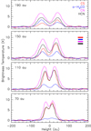 |
Fig. A.1 Cut in the tomographies at various radii for the brighter lines detected using Band 7. Color bars indicate their respective linear resolutions. |
A.3 Tomographies
In a rotating disk, the velocity along the line-of-sight projects as the impact parameter therefore each radius appears as a straight line in the Position-Velocity diagram. This allows a direct reconstruction of the 2D brightness distribution (Dutrey et al. 2017). The tomography has a constant linear resolution as a function of height above the disk plane, but a radius dependent linear resolution decreasing with increasing radius. It happens because the Keplerian shear is decreasing with radius compared to the finite local line width (Dutrey et al. 2017). Thus, we used the best available spectral resolution to compute the tomography. As the original beam is essentially elongated parallel to the mid-plane, the vertical resolution is given by the beam minor axis, and is about 22 au at the assumed distance (to compare with 60 au for the older low resolution data).
Figure 1 shows the tomographies with estimates of the tomographic radial resolution. Note that we did not attempt to correct for line opacity, neither for deviations from the Rayleigh Jeans law. To ease the comparison of the tomographies, Fig. 2 presents the superimposition of the main molecule emission (in contours) to the 13 CO tomography (in color).
Fig. A.1 presents vertical cuts, revealing double Gaussian shapes for vertical distributions. We model these at each radius by fitting two Gaussian, symmetric about the mid-plane in height and width, but of separate intensities:

The results of these fits are displayed in Fig. 3 and Figs. A.2–A.4 as a function of radius. Figure 3 shows the altitude A(r) and the deconvolved thickness, Fig. A.2 the peak brightness max(Is(r), In(r)), while Fig. A.3 displays the intensity ratio of both sides, Is(r)/In(r). The apparent (FWHM) width, 2√log(2) W ( r ), is displayed in Fig. A.4. The intrinsic thickness displayed in Fig. 3 is recovered from this FWHM by correcting for the beam size (assuming Gaussian shapes), using the clean beam minor axis since synthesized beams are elongated almost parallel to the disk plane.
Appendix B Individual molecule fitting
Geometry and velocity for the Flying Saucer disk.
For CS, ortho- and para-H2CO, and C3H2, several transitions were observed and fit together, allowing a derivation of the rotation temperature for these molecules. Cyclic C3H2 has transitions of its ortho and para forms at identical frequencies: we thus had to assumed an ortho-to-para ratio of 3, the high temperatures limit due to spin statistic, which is justified since the ground state of ortho-c-C3H2 lies only 2.3 K above that of para-c-C3H2, see Park et al. (2006).
The two rotational transitions of CN were fit separately, and an accurate separation of opacity from excitation temperature is possible for each of them because of their complex hyperfine structures, with hyperfine components spanning 1 to 2 orders of magnitude in opacity. The excellent agreement between both lines indicate that the emission is thermalized.
Only one transition is available for HCN, which has faint hyperfine structure, so that the derived temperature is based on the optically thick region within r < 150 au. DCN and N2D+ lines are too optically thin, the temperature had to be assumed. We have chosen to present in Table 1 the models assuming the mid-plane temperature (10 K) found in Paper I, such a temperature being more representative of location of DCN and N2D+ near the mid-plane. Note that assuming 17 K (the derived molecular layer temperature) provides derived surface densities which are only 30% smaller.
The stronger lines (13CO, CS, HCN) are optically thick up to about 150-200 au, allowing the temperature to be determined. The derived surface density profiles for these molecules is determined from the optically thin region outward under the assumption that the temperature law remains valid (see Piétu et al. 2007, for details, in particular their Fig. 4).
For C18O, the temperature was assumed identical to that of 13 CO.
Both 13CO and C18O lines are affected by background cloud emission, in ranges 3.1 to 4.6, and 4.1 to 4.6 km.s−1, respectively and the contaminated velocities have been ignored in the fit. For 12 CO, we used results from the more elaborate model of Guilloteau et al. (2025) that uses a vertical temperature gradient and accounts for the background emission.
Our disk model is relatively inappropriate for H2CO, whose emission is dominated by the outer regions and almost reaches the disk mid-plane. The best fit solutions thus leave some residuals for one of the three bright lines. The ortho-H2CO results seem more influenced by emission from the common molecular layer, in particular the transition at 351.768 GHz, while para-H2CO has a larger contribution from the outer parts.
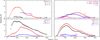 |
Fig. A.2 Apparent peak brightness max(Is(r), In(r)) as a function of radius. The cyan bar indicates the dust disk edge. |
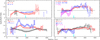 |
Fig. A.3 South-to-north layer brightness ratio Is(r)/In(r). The cyan bar indicates the dust disk edge. |
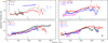 |
Fig. A.4 Apparent thickness (full width at half maximum) of the molecular layer 2 √log(2) W(r) as a function of radius. The black curve is the HCN(4-3) thickness for comparison. |
All Tables
All Figures
|
Fig. 1 Tomographic view of the observed spectral lines showing the mean brightness as a function of radius and height (both in au). Original beam sizes are indicated in the upper-right corner of each panel. CN hyperfine transitions are labeled by their frequency in MHz. Contour levels are 0.5-2 by 0.5, 3-10 by 1, and 12-30 by 2 K (except for the weak para-H2CO line, contour, at 0.25 K only). The panel labeled “CN Singles” shows a weighted average of three unblended lines at 338 516, 340 008, and 340 019 MHz, which is shown with a contour step of 0.25 K. The continuum at 230 GHz is shown in the bottom-left panel with contour levels 0.1, 0.2, 0.4, 0.8, and 1.2 K. |
| In the text | |
|
Fig. 2 13 CO tomography in false color with superimposition of the tomographies (black contours) of HCN 4-3, CS 7-6, and CN at 340.348 GHz; p-H2CO at 218.222 GHz; and DCN 3-2 and N2D+ 3-2. Contours are in steps of 1.5 K for HCN, CS, CN, and p-H2CO; 0.75 K for DCN; and 0.375 K for N2D+. The gray ellipses indicate the impact of line width on the effective beam at 80 and 240 au |
| In the text | |
|
Fig. 3 Top: altitude A(r) of the molecular layer as a function of radius. The black curve is the HCN(4-3) altitude for comparison. The cyan region indicates the approximate size of the dust disk. The dotted line corresponds to z/r = 0.2. Bottom: deconvolved thickness of the molecular layer. The deconvolution has been done assuming Gaussian shapes using the clean beam minor axis since synthesized beams are elongated almost parallel to the disk plane. The black curve is the HCN(4-3) thickness, for comparison. The cyan bar marks the edge of the dust disk. |
| In the text | |
|
Fig. 4 Profiles resulting from DISKFIT at 100 au. The green curve is the temperature profile, and the cyan curves indicate the H2 density structure (thin: under isothermal assumption at the mid-plane temperature (10 K); thick: using the full temperature profile) that were derived from the CO analysis by Guilloteau et al. (2025). The other colored curves are the molecular density profiles for CS (red), HCN (black), CN 2-1 (blue), and 3-2 (magenta) and are based on the parameters from Table 1. The corresponding horizontal bars indicate the measured temperatures and the density weighted average height of the emission. |
| In the text | |
|
Fig. 5 Tomographies of the residuals of the DISKFIT models. For each line, the best-fit model visibilities are subtracted from the observed ones and imaged as done for observations. The tomographic method is then applied on these residual data cubes. Contour spacings are 0.5 K. |
| In the text | |
|
Fig. A.1 Cut in the tomographies at various radii for the brighter lines detected using Band 7. Color bars indicate their respective linear resolutions. |
| In the text | |
|
Fig. A.2 Apparent peak brightness max(Is(r), In(r)) as a function of radius. The cyan bar indicates the dust disk edge. |
| In the text | |
|
Fig. A.3 South-to-north layer brightness ratio Is(r)/In(r). The cyan bar indicates the dust disk edge. |
| In the text | |
|
Fig. A.4 Apparent thickness (full width at half maximum) of the molecular layer 2 √log(2) W(r) as a function of radius. The black curve is the HCN(4-3) thickness for comparison. |
| In the text | |
Current usage metrics show cumulative count of Article Views (full-text article views including HTML views, PDF and ePub downloads, according to the available data) and Abstracts Views on Vision4Press platform.
Data correspond to usage on the plateform after 2015. The current usage metrics is available 48-96 hours after online publication and is updated daily on week days.
Initial download of the metrics may take a while.