| Issue |
A&A
Volume 704, December 2025
|
|
|---|---|---|
| Article Number | A310 | |
| Number of page(s) | 6 | |
| Section | Cosmology (including clusters of galaxies) | |
| DOI | https://doi.org/10.1051/0004-6361/202555791 | |
| Published online | 18 December 2025 | |
Constraints on AvERA cosmologies from cosmic chronometers and type Ia supernovae
1
Institute of Physics and Astronomy, ELTE Eötvös Loránd University, 1117 Budapest, Hungary
2
HUN-REN–ELTE Extragalactic Astrophysics Research Group, 1117 Budapest, Hungary
3
Department of Physics of Complex Systems, ELTE Eötvös Loránd University, 1117 Budapest, Hungary
4
Department of Physics, University of Helsinki, Gustaf Hällströmin katu 2, FI-00014 Helsinki, Finland
5
Institute for Astronomy, University of Hawaii, 2680 Woodlawn Drive, Honolulu, HI 96822, USA
★ Corresponding author: This email address is being protected from spambots. You need JavaScript enabled to view it.
Received:
3
June
2025
Accepted:
4
November
2025
Abstract
We constrain AvERA cosmologies in comparison with the flat Λ-cold dark matter (ΛCDM) model using cosmic chronometer (CC) data and the Pantheon+ sample of type Ia supernovae (SNe Ia). The analysis includes fits to both CC and SN datasets using the dynesty dynamic nested sampling algorithm. For the model comparison, we used the Bayesian model evidence and Anderson-Darling tests applied to the normalized residuals to assess consistency with a standard normal distribution. Best-fit parameters were derived within the redshift ranges z ≤ 2 for CCs and z ≤ 2.3 for SNe. For the baseline AvERA cosmology, we obtained best-fit values of the Hubble constant of H0 = 68.32−3.27+3.21 km s−1 Mpc−1 from the CC analysis and H0 = 71.99−1.03+1.05 km s−1 Mpc−1 from the SN analysis, each consistent within 1σ with the corresponding AvERA simulation value of H(z = 0). While both the CC and SN datasets yield higher Bayesian evidence for the flat ΛCDM model, they favor the AvERA cosmologies according to the Anderson-Darling test. We have identified signs of overfitting in each model, which suggests the possibility of overestimating the uncertainties in the Pantheon+ covariance matrix.
Key words: cosmological parameters
MTA Guest Professor 2023.
© The Authors 2025
 Open Access article, published by EDP Sciences, under the terms of the Creative Commons Attribution License (https://creativecommons.org/licenses/by/4.0), which permits unrestricted use, distribution, and reproduction in any medium, provided the original work is properly cited.
This article is published in open access under the Subscribe to Open model. This email address is being protected from spambots. You need JavaScript enabled to view it. to support open access publication.
1. Introduction
The Hubble tension is the most notable discrepancy of modern cosmology. The expansion rate measured from late-time and early-time observations shows a 4 − 6σ deviation (Riess 2020) if the standard Λ-cold dark matter (ΛCDM; see Peebles & Ratra 2003 for a review) cosmological model is used to compare the observations (Hu & Wang 2023). Measurements from the cosmic microwave background (CMB) suggest a lower H0 value (Planck Collaboration VI 2020), while local Universe observations, such as type Ia supernovae (Riess et al. 2022; Breuval et al. 2024), indicate a higher expansion rate. This inconsistency challenges our understanding of the Universe’s expansion history and suggests potential new physics beyond the ΛCDM paradigm. To address this tension, alternative cosmological models such as the timescape and backreaction models have been proposed. The timescape model introduced by Wiltshire (2007) posits that the Universe’s inhomogeneous structure leads to differential aging in regions of varying gravitational potential. This model suggests that the observed acceleration of cosmic expansion could be attributed to time dilation effects in low-density voids, thereby reconciling the disparate H0 measurements. Similarly, the backreaction models (Buchert 2000; Buchert et al. 2015) emphasize the influence of cosmic inhomogeneities on the Universe’s average expansion rate. By accounting for the effects of large-scale structures, such as voids and clusters, this model challenges the assumption of a perfectly homogeneous Universe inherent in the ΛCDM framework. Incorporating backreaction effects can add late-time complexity to the expansion history, and it can adjust the effective Hubble constant, potentially resolving the observed tension between early and late Universe measurements. These models offer promising avenues for resolving the Hubble tension, highlighting the need for a deeper understanding of cosmic inhomogeneities and their impact on the Universe’s expansion dynamics.
Average expansion rate approximation (AvERA) cosmology is a statistical, non-perturbative approach to model the cosmic backreaction (Rácz et al. 2017). It builds on the general relativistic separate Universe conjecture, which states that spherically symmetric regions in an isotropic Universe behave as independent mini-Universes with their own energy density – a concept proven by Dai, Pajer, and Schmidt (Dai et al. 2015). The AvERA approach uses these local densities to compute local expansion rates from the Friedmann equations and performs spatial averaging to estimate the overall expansion rate.
Local inhomogeneities influence the global expansion rate due to the nonlinearity of Einstein’s equations (Buchert et al. 2018). Under the AvERA approximation, the non-Gaussian distribution of matter and the growing low-density void regions cause the expansion to accelerate even with the flat ΩΛ = 0 initial conditions. Consequently, this approach has the potential to eliminate the need for dark energy – an unknown form of energy introduced within the concordance ΛCDM model – to explain cosmic evolution. Furthermore, Rácz et al. (2017) concluded that AvERA cosmology can resolve the Hubble tension.
The AvERA code is a collisionless N-body simulation that estimates the scale factor increment at each time step by averaging the local volumetric expansion rates of small subvolumes. Although local redshift evolution can vary across regions, the simulation uses a single global time step and applies a homogeneous rescaling of distances and velocities based on the effective scale factor, ensuring a one-to-one correspondence between time and redshift.
Within the AvERA framework, no closed-form analytic expression is available to describe the expansion history of the Universe. Instead, each simulation outputs tabulated redshifts, z, and Hubble parameters, H(z), at discrete time steps. The particle mass, corresponding to a coarse graining scale, is an adjustable parameter, that correlates with the matter density and thereby sets the expansion function, E(z). According to Rácz et al. (2017) the simulations were run with four different settings, using {135, 320, 625, 1080}×103 particles that correspond to {9.4, 3.96, 2.03, 1.17}×1011 M⊙ coarse graining scales, within a comoving volume of 147.623 Mpc3. The overall expansion amplitude was fixed by anchoring the Hubble parameter at z = 9 to H(z = 9) = 1191.9 km s−1 Mpc−1, complying with the Planck ΛCDM best-fit parameters – thereby ensuring consistency with CMB measurements. Consequently, different coarse graining scale settings lead to different present-day Hubble constants, H0, model (listed in Table 4).
In this paper, we use the four simulation outputs to test and constrain the AvERA cosmology with cosmic chronometers (CCs) and type Ia supernovae (SNe Ia). We probe E(z) = H(z)/H0, model evaluated at the data redshifts (by linear interpolation), while treating H0 as a free parameter. This separation enables a shape-only analysis, independent of the Planck-calibration. Agreement between the fit H0 and H0, model then indicates that AvERA, under that coarse graining setting, is simultaneously consistent with the dataset and the CMB. In both tests, we compare the performance of the AvERA cosmologies to that of the flat ΛCDM model. Sections 2 and 3 present the analyses and test results for CCs and SNe Ia, respectively, while Section 4 discusses our findings and summarizes our conclusions. Hereafter, we refer to AvERA cosmology as “the AvERA model”.
2. Test with cosmic chronometers
Under the assumption of the Friedmann-Lemaître-Robertson-Walker metric, the Hubble parameter is given by
The CC method, originally introduced by Jimenez & Loeb (2002) as the differential age method, estimates dz/dt by measuring the age and redshift differences (Δt and Δz, respectively) between two ensembles of passively evolving massive galaxies that are separated by a small redshift interval. The dominant source of measurement uncertainty typically arises from the determination of Δt.
For our analysis, we used the most up-to-date compilation of H(z) measurements obtained with the CC method (Simon et al. 2005; Stern et al. 2010; Moresco et al. 2012, 2016; Zhang et al. 2014; Moresco 2015; Ratsimbazafy et al. 2017; Borghi et al. 2022; Tomasetti et al. 2023) as listed in Table 1 of Moresco (2024). Among the three flagged data points that should not be used jointly in an analysis – because they are based on the same (or calibrated on the same) sample but obtained with different methods – we retained only the one originally included in Table 1 of Moresco et al. (2022). We therefore used a total of 33 CC data points.
From the AvERA simulation outputs, we obtained H(zi)sim at the CC redshifts, zi (with i indexing the individual CC data points), by linear interpolation between the two adjacent tabulated values bracketing zi. Although H(z)sim appears to be nearly linear across the CC redshift range (see Figure 1) and the simulation grid is reasonably dense, we estimated an upper bound on the interpolation error. This was quantified by comparing, at each tabulated redshift, the exact H(z)sim value with that obtained by interpolating between its two neighboring H(z)sim points. The relative deviation was calculated as |H(z)sim/H(z)sim, interp − 1|. Across the CC redshift range, it remained below 0.12% at maximum and below 0.03% on average. We therefore conclude that linear interpolation provides sufficient accuracy for our analysis, and thus does not affect our conclusions.
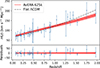 |
Fig. 1. Thirty-three CC data points from Table 1 of Moresco (2024) (blue dots with error bars), shown together with the best-fit H(z) curves for the AvERA-625k model (solid red curve with 1σ confidence bands) and the flat ΛCDM model (dash-dotted black curve). The lower panel displays the residuals after subtracting the best-fit AvERA-625k H(z) curve. The best-fit parameters for both models are given in Table 1. “625k” indicates the particle number used in the AvERA simulation. |
The expansion function at the ith CC redshift, zi, is then
 (1)
(1)
and the model H(z) used for testing is
 (2)
(2)
The H(z) function for the flat ΛCDM model is given by
 (3)
(3)
where Ωm, 0 is the present-day matter density parameter and H0 are free parameters. The contribution of radiation to the total density is neglected.
In our analysis, we fit H0 for the AvERA model, and H0 and Ωm, 0 for the flat ΛCDM model, to the CC data using the dynesty (Speagle 2020) Python package for dynamic nested sampling. We adopted uniform priors for all fits, with H0 ∼ 𝒰(50, 80) km s−1 Mpc−1 and Ωm, 0 ∼ 𝒰(0, 1). The parameters were constrained by minimizing
 (4)
(4)
where ΔD is the vector of 33 residuals, with the ith component given by
 (5)
(5)
and Cstat + syst is the full statistical and systematic covariance matrix. Instructions on how to properly estimate the CC total covariance matrix and incorporate it into a cosmological analysis are provided in the GitLab repository1, as is referenced in Moresco (2024).
The 33 CC data points used for the fitting, along with their statistical errors, are shown in Figure 1. Figure 1 also displays the best-fit H(z) curves for the AvERA-625k model and the flat ΛCDM model, where “625k” refers to the particle number used in the AvERA simulation. The best-fit parameter values and their uncertainties, given as the 16th, 50th, and 84th percentiles of the parameter posteriors, are presented in Table 1, while corner plots of the posteriors are available in our public code repository2 (Pataki et al. 2025). Our best-fit H0 and Ωm, 0 values in the flat ΛCDM model are consistent with the results of Moresco (2023), where H0 = 66.7 ± 5.3 km s−1 Mpc−1 (within 0.015σ) and  (within 0.06σ).
Model fit and test results for CC data.
In addition to parameter posterior estimation, the dynesty fit also yields the logarithm of the Bayesian evidence, log Z, which quantifies the marginal likelihood of the data under each model. These values enable direct model comparison via the Bayes factor, defined as log10ℬ = log10(Zmax/Z), where Zmax is the highest evidence value among the models considered. For model testing and comparison, we also adopted the Anderson-Darling (AD) test for normality (Anderson & Darling 1952; The MathWorks Inc. 2024), following the recommendations of Andrae et al. (2010). With this test, we evaluate a key property expected of a statistically valid model: that the fit residuals, once normalized by their observational uncertainties, are consistent with a standard normal distribution. A model is considered consistent with the null hypothesis of being the true model if the AD test yields a p value of p ≥ 0.05. For the model comparison, we defined Bayes factors from the AD test as log10ℬ = log10(pmax/p), where pmax is the highest p value among the tested models. While log Z is based on the likelihood and thus on the χ2 statistics – which compresses all residual deviations into a single scalar – the AD test directly probes the full shape of the normalized residual distribution. This enables a more detailed statistical assessment of model performance and makes the AD test particularly sensitive to overfitting effects, as we discuss in Section 3. The χ2 values, along with the Bayes factors from both nested sampling and the AD test, are reported in Table 1.
The model evidence derived from nested sampling indicates weak preferences for the flat ΛCDM model over all AvERA models (see Table 1). According to the AD test, both the AvERA and the flat ΛCDM models satisfy the p ≥ 0.05 criterion, with the AvERA model being slightly favored by the CC data. The AD test results show no significant differences between the various AvERA models with different coarse graining scale settings. However, only the best-fit H0 values for the AvERA-320k and AvERA-625k models are consistent within 1σ with their corresponding simulated values of H0, model (see Table 4). This indicates that, for the 320k and 625k settings, the CC and CMB data are mutually consistent, whereas the CMB-calibrated 135k and 1080k models are incompatible with the CC dataset.
3. Test with type Ia supernovae
We tested and constrained the AvERA model and the flat ΛCDM model using the Pantheon+ sample3 of SNe Ia (Scolnic et al. 2022), which comprises 1701 light curves of 1550 SNe within z ≲ 2.3. Our methodology followed Brout et al. (2022a), where – building on Tripp (1998) and Kessler & Scolnic (2017) – the SN distance moduli were defined from the standardized SN brightnesses, using the parameters obtained from SALT2 light-curve fits (Guy et al. 2007; Brout et al. 2022b):
 (6)
(6)
where
 (7)
(7)
Here, the x0 amplitude, used as mB ≡ −2.5log10(x0), the x1 stretch, and the c color parameters are from the light-curve fits. α and β are global nuisance parameters, related to stretch and color, respectively. The parameter MB is the fiducial magnitude of a SN, and δbias is a correction term to account for selection biases. The term δhost is the luminosity correction for the mass step (Popovic et al. 2021), where γ quantifies the magnitude of the luminosity difference between SNe in high- and low-mass galaxies; M* is the stellar mass of the host galaxy in units of solar masses, while S ∼ 10 (corresponding to 1010 M⊙) and τ define the step location and the step width, respectively. Altogether mB, x1, c, δbias, and log10M* are available for each SN in the Pantheon+ database3, whereas the global nuisance parameters α, β, γ, and MB must be fit simultaneously with the cosmological parameters.
The model distance modulus is defined as
 (8)
(8)
where dL(z) is the luminosity distance. The AvERA model does not provide explicit information about the present curvature density parameter, Ωk, 0. However, within the redshift range of the Pantheon+ sample (z ≲ 2.3), dL(z) has a weak dependence on the Universe’s spatial geometry. Moreover, since the Hubble parameter values, H(z), obtained from the AvERA simulations already encode the effects of curvature through the model’s dynamics, the main curvature dependence is effectively incorporated into the integral for dL(z). Empirically, we also found that the explicit (geometrical) dependence of dL(z) on Ωk, 0 has a negligible impact on the best-fit parameters. Therefore, we have adopted the flat-Universe approximation in our analysis, and leave the determination of Ωk, 0 in the AvERA model for future work. The luminosity distance used in the fits, for both the AvERA and the flat ΛCDM models, is thus given by
 (9)
(9)
In this expression, we used the cosmological redshift of each SN host galaxy in the CMB frame, corrected for the peculiar velocity (denoted as zHD in the Pantheon+ dataset3; see Carr et al. 2022).
For the AvERA model, the expansion function, E(z), was computed as described in Section 2. Specifically, we evaluated E(zi) at each SN redshift, zi, using Equation (1), where the corresponding H(zi)sim values were obtained by linear interpolation between adjacent H(z)sim points in the simulation output. Across the SN redshift range, the maximum and average interpolation errors matched the CC values reported in Section 2. In this model, only one cosmological parameter, H0, was fit simultaneously with the SN parameters. For the flat ΛCDM model, E(z) is defined by Equation (3), leading to two free cosmological parameters: H0 and Ωm, 0.
Since the parameters MB and H0 are degenerate (see Eqs. (6), (8), and (9)), we followed Brout et al. (2022a) and, for the 77 SNe located in Cepheid hosts, we replaced the model distance modulus (μ(z)) with the Cepheid-calibrated host-galaxy distance modulus (μCepheid) provided by SH0ES (Riess et al. 2022). Parameter estimation was performed using dynesty (Speagle 2020), minimizing χ2 as defined in Equation (4), with
 (10)
(10)
representing the ith component of the SN residual vector. The full statistical and systematic covariance matrix, Cstat + syst, from Brout et al. (2022a)3 was used in the fits and already accounts for the uncertainties in Cepheid-calibrated host distances. Uniform priors were applied for all parameters, with ranges listed in Table 2.
Uniform prior ranges used in the SN fit.
In the determination of best-fit model parameters, we followed the approach of Amanullah et al. (2010), Riess et al. (2022), and others, by employing the sigma clipping technique during model fitting, iteratively removing data points that deviated more than 3σ from the global fits until no such outliers remained. This method, as has been demonstrated by simulations such as those by Kowalski et al. (2008), helps preserve the fit results in the absence of contamination, while mitigating the influence of any outliers. For the 1701 SN data points, sigma clipping eliminated N = {15,16,16,16} for the AvERA model with {135k,320k,625k,1080k} particles, and N = 15 for the flat ΛCDM model.
We present the best-fit parameters and their uncertainties, given as the 16th, 50th, and 84th percentiles of the parameter posteriors, along with the test statistics in Table 3. The posterior distribution plots are available in our public code repository2 (Pataki et al. 2025). Figure 2 shows the distance moduli for all 1701 SNe, computed using the best-fit SN parameters of the AvERA-625k model, together with the corresponding μ(z) curve based on the best-fit value of  . As is shown in Table 4, only the AvERA-625k model exhibits agreement within 1σ between the best-fit H0 and the simulated value H0, model, indicating that SN and CMB data are mutually consistent only under the 625k setting.
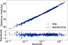 |
Fig. 2. Distance moduli for 1701 SN Ia observations (blue diamonds with error bars) and the AvERA-625k model (solid red curve), computed using the best-fit parameters (see Table 3). The SN data are from the Pantheon+ sample (Scolnic et al. 2022). The lower panel shows the residuals, obtained by subtracting the model μ(z) curve. |
Our best-fit H0 and Ωm, 0 values in the flat ΛCDM model are consistent with the results of Brout et al. (2022a), where H0 = 73.6 ± 1.1 km s−1 Mpc−1 (within 0.3σ) and Ωm, 0 = 0.334 ± 0.018 (within 0.2σ). Our H0 is also consistent with H0 = 73.30 ± 1.04 km s−1 Mpc−1 (within 0.1σ) and H0 = 73.04 ± 1.04 km s−1 Mpc−1 (within 0.06σ), obtained by Riess et al. (2022) with and without the inclusion of high-redshift (z ∈ [0.15, 0.8)) SNe, respectively. However our H0 in the flat ΛCDM model is in 4.8σ tension with the Planck+BAO H0 = 67.66 ± 0.42 km s−1 Mpc−1 (Planck Collaboration VI 2020), confirming the Hubble tension.
For the model comparison, we applied the same methods as in Section 2: model evidence and AD test to the residuals. The normalized residuals were computed as r = L−1ΔD, with Cstat + syst = LLT the Cholesky factorization of the covariance. The χ2 values, along with the Bayes factors derived from nested sampling and from the AD test, are reported in Table 3. Since the nested sampling evidence (log Z) was generated during the fitting process, we report log10ℬ (NS) values from the initial fit iteration, which used the complete SN dataset prior to any sigma clipping, in order to maintain consistency across all statistics.
Model fit and test results for SN Ia data.
Although none of the best-fit models satisfied the p ≥ 0.05 criterion for consistency with the SN data, the AD test-based Bayes factors indicate that the AvERA model is at least substantially favored over the flat ΛCDM model. As is shown in Table 3, this ranking is in contrast to that implied by the Bayes factors from nested sampling, which strongly favors the flat ΛCDM model. This discrepancy is due to the flat ΛCDM model overfitting the SN data, as is illustrated in Figure 3. The AD test is particularly sensitive to such effects, as it responds to subtle deviations from the expected normal distribution of residuals, which may not be captured by global statistics like χ2 or log Z. In the upper panel of Figure 3, we show the histogram of normalized residuals, which are expected to follow a standard normal distribution for the true model underlying the SN data. Both the flat ΛCDM and AvERA-625k models yield residuals that are overly concentrated near zero (i.e., under–dispersed relative to 𝒩(0, 1)), with sample standard deviations of σ = 0.93 and σ = 0.94, respectively. The lower panel of Figure 3 displays histograms of AD-test log10p values computed for half a million samples drawn from the joint posterior distributions of the SN fit. While none of the flat ΛCDM or AvERA realizations satisfy the p ≥ 0.05 (log10p ≥ −1.3) criterion, the preference for the AvERA model remains clearly evident. The highest (median) p value for the flat ΛCDM model is exceeded by {0.2%, 0.7%, 2.6%, 6.1%} ({64%, 69%, 71%, 73%}) of the p values for the AvERA model with {135k,320k,625k,1080k} particles.
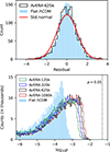 |
Fig. 3. Upper panel: Histograms of normalized residuals for the best-fit AvERA-625k and flat ΛCDM models, fit to the Pantheon+ SN Ia data (Scolnic et al. 2022). The red curve represents the standard normal distribution expected for the true model underlying the data. Lower panel: Histograms of AD-test log10p values for half a million realizations sampled from the joint posterior distributions. The dashed vertical line marks the significance threshold of p = 0.05 (log10p = −1.301) for consistency with the null hypothesis of being the true model. While none of the realizations reach this level, the preference for the AvERA model is clearly evident. |
Despite its lower χ2 value, the flat ΛCDM model is inconsistent with the Pantheon+ data according to the AD test. This is due to the model overfitting the SN data, potentially as a consequence of the error estimation strategy (Raffai et al. 2025). While conservative error estimation is generally a sound approach for robust parameter inference, it can result in the tested models overfitting data, potentially leading to false conclusions in model comparisons. Consistent with our finding, Keeley et al. (2024) also concluded that the flat ΛCDM model overfits the Pantheon+ SN data, hinting that SN measurement errors may have been conservatively overestimated. Another potential source of overfitting is that the preprocessed observational data may not be entirely independent from the concordance (flat ΛCDM) cosmological model. For example, as is noted by Carr et al. (2022), zHD values in the Pantheon+ dataset are corrected for peculiar velocities of SN host galaxies calculated by assuming flat ΛCDM cosmology. This model dependency may contribute to the flat ΛCDM model overfitting the SN data, although Carr et al. (2022) note that the cosmology-dependence of the correction is weak.
4. Conclusions
In Sections 2 and 3, we tested and compared the predictions of the AvERA model with those of the flat ΛCDM model. A comprehensive summary of our results is provided in Tables 1 and 3.
The CC and SN datasets favor the AvERA model over the flat ΛCDM model according to the AD test, but indicate a preference for the flat ΛCDM model based on the nested sampling evidence. Among the tested AvERA models, the 625k setting stands out: the simulated H0, model lies within the 1σ credible interval of the fit H0 in both the CC and SN analyses (Table 4). Since H0, model results from calibrating the simulation to the CMB, this concordance implies mutual consistency of the CC, SN, and CMB data under the AvERA-625k model; accordingly, we adopted it as our baseline AvERA model. Within this model, such concordance points to a potential alleviation of the Hubble tension – that is, the discrepancy between CMB- and SN-based determinations of H0.
Deviations in H0 between simulations and tests.
Only four outputs, corresponding to four discrete coarse graining settings, were available for this analysis; however, the true scale could in principle lie between them. To seek the optimal coarse graining scale, we performed a joint CC+SN fit for the AvERA model, treating the coarse graining scale as a free parameter. To achieve this, we applied linear interpolation between the four simulation outputs to compute the model H(z) for any integer particle number within the range [135k, 1080k]. In this analysis, the SN parameters were fixed to the average of their best-fit values from Table 3, as the table shows that these parameters vary only minimally across different graining scales. The implementation code and the corresponding corner plot are available in our code repository2 (Pataki et al. 2025). This analysis did not reveal a single preferred graining scale, as is indicated by the nearly uniform posterior distribution of the particle number. We obtained  km s−1 Mpc−1, which is in only 0.06σ tension with the simulated value of H0 for the AvERA-625k model, further supporting its choice as the baseline AvERA model.
Acknowledgments
The authors would like to thank Bence Bécsy for his assistance with dynesty. This project has received funding from the HUN-REN Hungarian Research Network and was also supported by the NKFIH excellence grant TKP2021-NKTA-64 and NKFI-147550. IS acknowledges NASA grants 80NSSC24K1489 and 24-ADAP24-0074 and thanks the hospitality of the MTA-CSFK Lendület “Momentum” Large-Scale Structure (LSS) Research Group at Konkoly Observatory supported by a Lendület excellence grant by the Hungarian Academy of Sciences (MTA). GR acknowledges the support of the Research Council of Finland grant 354905 and the support by the European Research Council via ERC Consolidator grant KETJU (no. 818930).
References
- Amanullah, R., Lidman, C., Rubin, D., et al. 2010, ApJ, 716, 712 [CrossRef] [Google Scholar]
- Anderson, T. W., & Darling, D. A. 1952, Ann. Math. Stat., 23, 193 [Google Scholar]
- Andrae, R., Schulze-Hartung, T., & Melchior, P. 2010, ArXiv e-prints [arXiv:1012.3754] [Google Scholar]
- Borghi, N., Moresco, M., & Cimatti, A. 2022, ApJ, 928, L4 [NASA ADS] [CrossRef] [Google Scholar]
- Breuval, L., Riess, A. G., Casertano, S., et al. 2024, ApJ, 973, 30 [Google Scholar]
- Brout, D., Scolnic, D., Popovic, B., et al. 2022a, ApJ, 938, 110 [NASA ADS] [CrossRef] [Google Scholar]
- Brout, D., Taylor, G., Scolnic, D., et al. 2022b, ApJ, 938, 111 [NASA ADS] [CrossRef] [Google Scholar]
- Buchert, T. 2000, Gen. Relat. Grav., 32, 105 [Google Scholar]
- Buchert, T., Carfora, M., Ellis, G. F. R., et al. 2015, Class. Quant. Grav., 32, 215021 [NASA ADS] [CrossRef] [Google Scholar]
- Buchert, T., Mourier, P., & Roy, X. 2018, Class. Quant. Grav., 35, 24LT02 [Google Scholar]
- Carr, A., Davis, T. M., Scolnic, D., et al. 2022, PASA, 39, e046 [NASA ADS] [CrossRef] [Google Scholar]
- Dai, L., Pajer, E., & Schmidt, F. 2015, JCAP, 2015, 059 [CrossRef] [Google Scholar]
- Guy, J., Astier, P., Baumont, S., et al. 2007, A&A, 466, 11 [NASA ADS] [CrossRef] [EDP Sciences] [Google Scholar]
- Hu, J.-P., & Wang, F.-Y. 2023, Universe, 9, 94 [CrossRef] [Google Scholar]
- Jimenez, R., & Loeb, A. 2002, ApJ, 573, 37 [NASA ADS] [CrossRef] [Google Scholar]
- Keeley, R. E., Shafieloo, A., & L’Huillier, B. 2024, Universe, 10, 439 [Google Scholar]
- Kessler, R., & Scolnic, D. 2017, ApJ, 836, 56 [Google Scholar]
- Kowalski, M., Rubin, D., Aldering, G., et al. 2008, ApJ, 686, 749 [NASA ADS] [CrossRef] [Google Scholar]
- Moresco, M. 2015, MNRAS, 450, L16 [NASA ADS] [CrossRef] [Google Scholar]
- Moresco, M. 2023, ArXiv e-prints [arXiv:2307.09501] [Google Scholar]
- Moresco, M. 2024, ArXiv e-prints [arXiv:2412.01994] [Google Scholar]
- Moresco, M., Cimatti, A., Jimenez, R., et al. 2012, JCAP, 2012, 006 [CrossRef] [Google Scholar]
- Moresco, M., Pozzetti, L., Cimatti, A., et al. 2016, JCAP, 2016, 014 [CrossRef] [Google Scholar]
- Moresco, M., Amati, L., Amendola, L., et al. 2022, Liv. Rev. Relat., 25, 6 [NASA ADS] [Google Scholar]
- Pataki, A., Raffai, P., Csabai, I., Rácz, G., & Szapudi, I. 2025, https://doi.org/10.5281/zenodo.15478706 [Google Scholar]
- Peebles, P. J., & Ratra, B. 2003, Rev. Mod. Phys., 75, 559 [NASA ADS] [CrossRef] [Google Scholar]
- Planck Collaboration VI. 2020, A&A, 641, A6 [NASA ADS] [CrossRef] [EDP Sciences] [Google Scholar]
- Popovic, B., Brout, D., Kessler, R., Scolnic, D., & Lu, L. 2021, ApJ, 913, 49 [NASA ADS] [CrossRef] [Google Scholar]
- Rácz, G., Dobos, L., Beck, R., Szapudi, I., & Csabai, I. 2017, MNRAS, 469, L1 [Google Scholar]
- Raffai, P., Pataki, A., Böttger, R. L., Karsai, A., & Dálya, G. 2025, ApJ, 979, 51 [Google Scholar]
- Ratsimbazafy, A. L., Loubser, S. I., Crawford, S. M., et al. 2017, MNRAS, 467, 3239 [NASA ADS] [CrossRef] [Google Scholar]
- Riess, A. G. 2020, Nat. Rev. Phys., 2, 10 [NASA ADS] [CrossRef] [Google Scholar]
- Riess, A. G., Yuan, W., Macri, L. M., et al. 2022, ApJ, 934, L7 [NASA ADS] [CrossRef] [Google Scholar]
- Scolnic, D., Brout, D., Carr, A., et al. 2022, ApJ, 938, 113 [NASA ADS] [CrossRef] [Google Scholar]
- Simon, J., Verde, L., & Jimenez, R. 2005, Phys. Rev. D, 71, 123001 [NASA ADS] [CrossRef] [Google Scholar]
- Speagle, J. S. 2020, MNRAS, 493, 3132 [Google Scholar]
- Stern, D., Jimenez, R., Verde, L., Stanford, S. A., & Kamionkowski, M. 2010, ApJS, 188, 280 [NASA ADS] [CrossRef] [Google Scholar]
- The MathWorks Inc. 2024, adtest, MATLAB Version: 24.1.0.2628055 (R2024a) Update 4 [Google Scholar]
- Tomasetti, E., Moresco, M., Borghi, N., et al. 2023, A&A, 679, A96 [NASA ADS] [CrossRef] [EDP Sciences] [Google Scholar]
- Tripp, R. 1998, A&A, 331, 815 [NASA ADS] [Google Scholar]
- Wiltshire, D. L. 2007, Phys. Rev. Lett., 99, 251101 [Google Scholar]
- Zhang, C., Zhang, H., Yuan, S., et al. 2014, Res. Astron. Astrophys., 14, 1221 [CrossRef] [Google Scholar]
All Tables
All Figures
|
Fig. 1. Thirty-three CC data points from Table 1 of Moresco (2024) (blue dots with error bars), shown together with the best-fit H(z) curves for the AvERA-625k model (solid red curve with 1σ confidence bands) and the flat ΛCDM model (dash-dotted black curve). The lower panel displays the residuals after subtracting the best-fit AvERA-625k H(z) curve. The best-fit parameters for both models are given in Table 1. “625k” indicates the particle number used in the AvERA simulation. |
| In the text | |
|
Fig. 2. Distance moduli for 1701 SN Ia observations (blue diamonds with error bars) and the AvERA-625k model (solid red curve), computed using the best-fit parameters (see Table 3). The SN data are from the Pantheon+ sample (Scolnic et al. 2022). The lower panel shows the residuals, obtained by subtracting the model μ(z) curve. |
| In the text | |
|
Fig. 3. Upper panel: Histograms of normalized residuals for the best-fit AvERA-625k and flat ΛCDM models, fit to the Pantheon+ SN Ia data (Scolnic et al. 2022). The red curve represents the standard normal distribution expected for the true model underlying the data. Lower panel: Histograms of AD-test log10p values for half a million realizations sampled from the joint posterior distributions. The dashed vertical line marks the significance threshold of p = 0.05 (log10p = −1.301) for consistency with the null hypothesis of being the true model. While none of the realizations reach this level, the preference for the AvERA model is clearly evident. |
| In the text | |
Current usage metrics show cumulative count of Article Views (full-text article views including HTML views, PDF and ePub downloads, according to the available data) and Abstracts Views on Vision4Press platform.
Data correspond to usage on the plateform after 2015. The current usage metrics is available 48-96 hours after online publication and is updated daily on week days.
Initial download of the metrics may take a while.