| Issue |
A&A
Volume 704, December 2025
|
|
|---|---|---|
| Article Number | A237 | |
| Number of page(s) | 12 | |
| Section | Planets, planetary systems, and small bodies | |
| DOI | https://doi.org/10.1051/0004-6361/202555940 | |
| Published online | 19 December 2025 | |
A kinematic history of stellar encounters with Beta Pictoris
1
Centro de Astrobiología (CAB), CSIC-INTA,
Camino Bajo del Castillo s/n,
28692,
Villanueva de la Cañada, Madrid,
Spain
2
Departamento de Física de la Tierra y Astrofísica, Facultad de Ciencias Físicas, Universidad Complutense de Madrid,
28040
Madrid,
Spain
3
Institute of Science and Technology Austria (ISTA),
Am Campus 1,
3400
Klosterneuburg,
Austria
4
Lund Observatory, Division of Astrophysics, Department of Physics, Lund University,
Box 118,
221 00
Lund,
Sweden
5
Instituto de Astrofísica de Canarias,
38200
La Laguna, Tenerife,
Spain
6
Universidad de La Laguna (ULL), Astrophysics Department,
38206 La Laguna, Tenerife,
Spain
★ Corresponding author: This email address is being protected from spambots. You need JavaScript enabled to view it.
Received:
13
June
2025
Accepted:
30
September
2025
Abstract
Context. Beta Pictoris is an A-type star that hosts a complex planetary system with two massive gas giants and a prominent debris disc. Variable absorption lines in its stellar spectrum have been interpreted as signatures of exocomets – comet-like bodies transiting the star. Stellar flybys can gravitationally perturb objects in the outer comet reservoir, altering their orbits and potentially injecting them into the inner system, thereby triggering exocomet showers.
Aims. We assessed the contribution of stellar flybys to the observed exocomet activity by reconstructing the stellar encounter history of β Pictoris in the past and future.
Methods. We used Gaia DR3 data, supplemented with radial velocities from complementary spectroscopic surveys, to compile a catalogue of stars currently within 80 pc of β Pictoris. Their orbits were integrated backwards and forwards in time in an axisymmetric Galactic potential (via the GALA package) to identify encounters within 2 pc of the system.
Results. We identified 99 416 stars currently within 80 pc of β Pictoris with resolved kinematics. Among these, 49 stars (including the eight components of five binaries) encounter β Pictoris within 2 pc between –1.5 Myr and +2 Myr. For four of the binaries, the centre-of-mass trajectories also pass within 2 pc. We estimated the sample to be more than 60% complete within 0.5 Myr of today.
Conclusions. Despite β Pictoris being the eponym of its famous moving group, none of the identified encounters involved its moving group members; all are unrelated field stars. We found no encounter capable of shaping the observed disc structures, although stellar flybys may contribute to the long-term evolution of an Oort Cloud-like structure. Our catalogue constitutes the most complete reconstruction of the β Pictoris encounter history to date and provides a robust foundation for future dynamical simulations.
Key words: catalogs / comets: general / Oort Cloud / stars: kinematics and dynamics / stars: individual: β Pictoris
© The Authors 2025
 Open Access article, published by EDP Sciences, under the terms of the Creative Commons Attribution License (https://creativecommons.org/licenses/by/4.0), which permits unrestricted use, distribution, and reproduction in any medium, provided the original work is properly cited.
This article is published in open access under the Subscribe to Open model. This email address is being protected from spambots. You need JavaScript enabled to view it. to support open access publication.
1 Introduction
The β Pictoris system (hereafter β Pic) is one of the most iconic examples of a young, dynamically evolving planetary system. It offers a valuable laboratory for investigating planet formation, disc evolution, and exocomet activity. Located at 19.6 pc from the Sun (Gaia Collaboration 2016b; Lindegren et al. 2021b), β Pic is a ~20 Myr-old A6V-type star (Couture et al. 2023; Gray et al. 2006) and the namesake of the β Pic Moving Group (β PMG), whose members share common kinematics and likely originated in the same star-forming region (Zuckerman et al. 2001; Couture et al. 2023; Lee et al. 2024; Lee & Song 2024).
Beta Pic hosts a prominent edge-on debris disc, first imaged by Smith & Terrile (1984), which has been the focus of extensive study due to its structure. High-resolution observations have revealed a complex morphology, including a primary disc and an inclined secondary component (Heap et al. 2000), along with warps, clumps, and large-scale asymmetries (Golimowski et al. 2006; Lagrange et al. 2012). Using Atacama Large Millimeter Array imaging, Dent et al. (2014) and Matrà et al. (2019) traced a planetesimal belt extending from ~50 to 150 au, with ongoing dust production attributed to collisional cascades and comet-like activity (Thébault & Beust 2001; Tobin et al. 2019). In addition to dust, the disc contains a significant amount of CO and atomic carbon gas (Lagrange et al. 1995; Cataldi et al. 2018), which is atypical for systems of comparable ages.
Recent JWST observations (Rebollido et al. 2024) have revealed a large, asymmetric dust feature – nicknamed the ‘Cat’s tail’ – originating from the secondary disc. This structure likely results from a recent collisional or outgassing event and is associated with a region with a higher density of circumstellar gas (Dent et al. 2014). Mid-infrared spectroscopy shows that the hot crystalline dust features present in 2004–2005 have since disappeared, consistent with a major collision followed by the radiation-pressure blowout of small grains (Chen et al. 2024). Spectroscopic monitoring of the system has also revealed transient absorption features attributed to exocomets transiting the stellar disc (Ferlet et al. 1987; Beust et al. 1990; Kiefer et al. 2014; Lecavelier des Etangs et al. 2022; Hoeijmakers et al. 2025), reinforcing the interpretation of a highly active and dynamically rich environment.
The system also hosts two directly imaged giant exoplanets. Beta Pic b, with a mass of 12 MJup and an orbital distance of 10 au, was one of the first exoplanets discovered via direct imaging (Lagrange et al. 2009a,b, 2010). Beta Pic c, a closer-in giant of 9 MJup at 2.7 au, was detected through a combination of radial velocity (RV) measurements and direct imaging (Lagrange et al. 2019; Nowak et al. 2020). Both planets have inclinations of ~89° (Lacour et al. 2021) and are aligned with the main disc but misaligned with the secondary disc (Rebollido et al. 2024). They were proposed – prior to their discovery – to be dynamical sculptors of the observed warps and resonant structures of the surrounding disc (Mouillet et al. 1997). Numerical simulations suggest that their gravitational influence can perturb planetesimals onto star-grazing orbits via mean-motion resonances, potentially explaining the observed exocomet activity (Thébault & Beust 2001; Beust et al. 2024).
Given the presence of giant planets and an extended planetesimal disc, it is plausible that β Pic hosts a distant, dynamically evolving reservoir of icy bodies – an analogue to the Solar System’s Oort Cloud. In the Solar System, the Oort Cloud is thought to have formed through a combination of scattering by giant planets and external perturbations from the Galactic tidal field and stellar encounters (Oort 1950; Dones et al. 2004; Brasser et al. 2008; Brasser & Morbidelli 2013; Nesvornỳ 2018; Shannon et al. 2019). Several studies have used N-body simulations to explore the formation and evolution of such reservoirs (Levison et al. 2004; Fouchard et al. 2006; Kaib & Quinn 2008; Morbidelli 2005; Torres et al. 2019; Vokrouhlickỳ et al. 2019; Portegies Zwart et al. 2021). Unlike the Oort Cloud – which has had billions of years to reach a dynamically relaxed state – the cometary cloud around β Pic would at present be dynamically unevolved, potentially resembling a proto-Oort Cloud in its formative stages. Studies of the influence of stellar encounters on this distant reservoir in the Solar System (Rickman 1976; García-Sánchez et al. 1999; Bailer-Jones 2015, 2018; Bailer-Jones et al. 2018; Torres et al. 2019) often employ the impulse approximation (Oort 1950; Rickman 1976; Dybczyński 1994; Binney & Tremaine 2011) as an alternative to full N-body simulations to study the dynamical effect induced by a fast-moving stellar perturber, reducing the three-body Sun–star–comet problem to the net impulse transferred by the star to the Sun and the comet.
Kalas et al. (2001) conducted an early investigation of the encounter history of β Pic using astrometric data from the HIPPARCOS catalogue (Perryman et al. 1997) and RVs from Barbier-Brossat & Figon (2000). They propagated the rectilinear trajectories of 21 497 stars and identified 18 candidates that passed within 5 pc of β Pic over the past 1 Myr. Applying the impulse approximation, they assessed the effects of these encounters on the eccentricities of a hypothetical cometary cloud and concluded that, if such a reservoir exists, past stellar encounters may have contributed to the formation and shaping of an Oort Cloud-like structure.
The data releases of the European Space Agency’s Gaia mission (Gaia Collaboration 2016b,a, 2018, 2021a, 2023) have enabled a major advance in our understanding of stellar dynamics in the solar neighbourhood. With astrometry data for 1.46 billion stars and RVs for 33 million, it is now possible to reassess the encounter history of β Pic with greatly improved precision and completeness.
The aim of this work is to construct the most complete and accurate catalogue to date of stellar encounters with β Pic, using Gaia astrometry and complementary RV data. Section 2 describes our catalogue of stars within 80 pc of β Pic and the selection criteria applied. Section 3 details the orbital integration of these stars to identify past and future encounters with β Pic; we also assessed the completeness of our results using encounter probability estimates and identified binary and higher-multiplicity systems within our sample. Section 4 compares our findings with the earlier study by Kalas et al. (2001). Finally, Sect. 5 presents our summary and conclusions.
2 The β Pictoris neighbourhood catalogue
To construct a catalogue of stars in the vicinity of β Pic, we began with Gaia data. The latest release, Gaia Data Release 3 (Gaia Collaboration 2023) was divided into two parts: the Early Data Release 3 (hereafter GEDR3; Gaia Collaboration 2021a), which provides astrometry (Lindegren et al. 2021b) and integrated photometry, and the full Gaia Data Release 3 (hereafter GDR3), which superseded GEDR3 and includes additional products such as RV data (Katz et al. 2023), spectra, astrophysical parameter tables, and results for non-single stars, among others. Also included in GEDR3 is the Gaia Catalogue of Nearby Stars (GCNS; Gaia Collaboration 2021b), a census of 331 312 Gaia sources that is volume-complete for spectral types earlier than M8 within a 100 pc radius centred on the Sun.
We applied the parallax correction from Lindegren et al. (2021a), the proper motion correction proposed by Cantat-Gaudin & Brandt (2021), and the uncertainty corrections for both parallax and proper motion as outlined by Maíz Apellániz (2022), using a Python function provided by M. Pantaleoni González (priv. comm.) to account for known systematics in the astrometric data. This method inflates the uncertainties according to the renormalised unit weight error of the source astrometry (ruwe), so the objects with poor solutions are assigned larger uncertainties.
As β Pic lies approximately 20 pc from the Sun, the largest sphere centred on β Pic that fits within the GCNS coverage has a radius of about 80 pc. We used the dedicated functions of the Tool for OPerations on Catalogues And Tables (TOP-CAT; Taylor 2005) to select sources within this region (see Appendix A). Our initial sample comprises 156 995 stars from the GCNS catalogue. Among these, 46 321 have complete 6D phase space information (right ascension, declination, parallax, proper motion, and RV) with associated errors and astrometric covariances. The RV data in GCNS are sourced from GDR2 and supplemented by references compiled in the Set of Identifications, Measurements and Bibliography for Astronomical Data (SIMBAD; Wenger et al. 2000).
To incorporate the latest RV data from Gaia (Katz et al. 2023), we crossmatched the GCNS sources with GDR3, which is straightforward as the two catalogues share the same Gaia source ID. This increased the number of sources with RVs to 95 453.
To further expand RV coverage, we crossmatched the GCNS sources with major spectroscopic surveys: The Sixth Data Release of the Radial Velocity Experiment (RAVE; Steinmetz et al. 2020), the Fourth Data Release of the GALactic Archaeology with HERMES (GALAH, Buder et al. 2025), the Seventeenth Data Release of the Apache Point Observatory Galactic Evolution Experiment (APOGEE; Abdurro’uf et al. 2022), and the Low Resolution Survey (LRS; Deng et al. 2012) and Medium Resolution Survey (MRS; Liu et al. 2020) of the Tenth Data Release of the Large Sky Area Multi-Object Fiber Spectroscopic Telescope (LAMOST). These catalogues include Gaia IDs, which were used for the crossmatch.
2.1 Selection filters
We applied quality filters to discard the poorest data, adapting the criteria proposed by Tsantaki et al. (2022) and following the documentation of each survey12 (Steinmetz et al. 2020; Luo et al. 2015):
RAVE: RV zero-point correction |cHRV| < 10 km s−1; RV error e_HRV < 8 km s−1; correlation coefficient R > 10; quality flag Qual ≠ 1; and a signal-to-noise ratio S_Nm > 0, which also flags errors when negative.
GALAH: Signal-to-noise per pixel snr_px_ccd3 > 30; stellar parameters quality flag flag_sp = 0; and RV error e_rv_comp_1 < 100 km s−1).
APOGEE: Quality flag STARFLAG mod 2flag ≠ 0, (keeping flags 0,3,4,9,12,13,19,22); signal-to-noise ratio SNR > 5; and RV error 0 km s−1 < VRELERR < 2 km s−1.
LAMOST-LRS: Signal-to-noise ratio snrg > 15; and RV error rv_err > 0 km s−1.
LAMOST-MRS: Signal-to-noise ratio snr > 15; and RV error 0 km s−1<rv_lasp1_err. < 100 km s−1.
RV data for the GCNS sources within 80 pc of β Pic.
2.2 Source catalogues and visit catalogues
The previously mentioned surveys conduct multiple observations of the same object to enhance result accuracy. Depending on the curation strategy, these are either merged into a single entry per source (hereafter referred to as ‘source catalogues’) or stored as multiple observations (hereafter referred to as ‘visit catalogues’). In our science case, we had to use the source catalogue to crossmatch between sources.
Gaia releases source catalogues, whereas LAMOST-LRS, LAMOST-MRS and RAVE provide visit catalogues. GALAH and APOGEE offer both types of catalogues. Following the recommendations for each survey, we used the APOGEE visit catalogue and the GALAH source catalogue.
Where necessary, we transformed visit catalogues into source catalogues. For each star, we computed the median RV from its visits. If the number of visits was even, instead of calculating the mean between the two central values, we selected the value with the smallest associated error. When multiple RV values were available from different surveys, we retained the one with the smallest error.
The main GDR3 table provides astrometric and RV data obtained by fitting the standard single-star model (Perryman et al. 1997) to the spacecraft measurements. As a first attempt to account for binaries, GDR3 also includes dedicated tables that refit poor astrometric results as accelerated models compatible with binaries (Halbwachs et al. 2023; Holl et al. 2023), and variable RVs as eclipsing or spectroscopic binaries (Gosset et al. 2025). When available, we replaced the original astrometric or RV entries with the corresponding binary solutions.
As with astrometry, RV data can not be used directly from the archive tables without correction for known systematics. For cool stars (rv_template_teff < 8500 K), we applied the prescription of Katz et al. (2023), for hot stars that of Blomme et al. (2023), and for the uncertainties the recipe of Babusiaux et al. (2023).
The final sample includes 99 416 sources within 80 pc of β Pic with RVs and associated uncertainties – representing 63.3% of the total GCNS sources in this volume. The remaining 57 579 (36.7%) lack RV data. The distribution of RV sources across surveys is summarised in Table 1. Note that the Gaia counts differ from those mentioned earlier in this section, as we adopted RV data from the other surveys when they offered lower uncertainties.
2.3 Convective blueshift and gravitational redshift
Spectroscopic RVs should not be used as kinematic RVs (Lindegren et al. 2003). Two main effects contribute to systematic shifts in the measured line positions: the gravitational redshift and the convective blueshift.
The gravitational redshift arises because photons lose energy when escaping from the stellar gravitational potential of the star, producing a systematic redshift that depends on the stellar mass and radius (see Couture et al. 2023), but in this work we adopted mass and log g due to data availability:
 (1)
(1)
The convective blueshift is related to the dynamics of convective atmospheres: hotter, rising gas contributes more flux than cooler, descending material, leading to asymmetric spectral lines and a net blueshift. Its amplitude depends on the stellar structure, which is significant in giants and cool dwarfs with outer convective layers, but negligible in hot dwarfs and white dwarfs. For the corrections, we followed the formulation of Couture et al. (2023) for dwarfs, and the dependence described by Liebing et al. (2023) for evolved stars. Typical values of the gravitational redshift are 0.4–0.6 km s−1, whereas the convective blueshift generally has lower absolute values, in the range 0.02–0.4 km s−1.
As a source of stellar parameters, we used the same spectroscopic surveys that provided RV data, complemented with the TESS Input Catalogue (TIC) values (Paegert et al. 2021), and additional works dedicated to white dwarfs (Gianninas et al. 2015; Bédard et al. 2017; Kilic et al. 2020; Bonavita et al. 2020; Jiménez-Esteban et al. 2023; Vincent et al. 2024). The TIC catalogue classifies stars as dwarfs (main-sequence and white dwarfs), giants, or subgiants (the last two being evolved stars). We also employed the luminosity classes of spectral types available in SIMBAD to complete the classification; objects without spectral type information were assumed to be dwarfs. Once classified, missing parameters were estimated by interpolation within each class: for evolved stars and white dwarfs we used available data for objects with similar known parameters, while for main-sequence dwarfs, we relied on the updated version3 of Table 3 of Pecaut & Mamajek (2013). Objects with no available data were assumed to be faint, low-mass stars and were assigned the corresponding gravitational redshift (0.4±0.3 km s−1) and convective blueshift (0.0 ± 0.2 km s−1), according to Couture et al. (2023).
After applying the corrections to all sources, the kinematic RVs can be used. The complete catalogue is available on Zenodo.
Galactic potential parameters of MilkyWayPotential2022.
3 Close encounters with β Pic
To calculate the stellar encounters with β Pic and its nearby stars, we traced their orbits backwards and forwards in time and calculated the minimum distance between their positions over time. In these integrations we neglected star-star interactions (see the discussion in Sect. 3.1), so each orbit was determined solely by its initial conditions and the Galactic potential. We used the Galactic potential MilkyWayPotential2022 presented in the Python package GALA (Price-Whelan 2017; Price-Whelan et al. 2020) to perform the integration of stellar motions within a Galaxy model. This potential comprises four components: a Hernquist bulge and nucleus, a Miyamoto-Nagai disc, and a Navarro– Frenk–White dark matter halo. The developers fitted the disc model to the Eilers et al. (2019) rotation curve for radial dependence, and its vertical structure was fitted to the phase-space spiral in the solar neighbourhood as described in Darragh-Ford et al. (2023)4. The parameters defining the potential are listed in Table 2.
Prior to integration, we transformed the Gaia coordinates into a Galactocentric reference frame using ASTROPY, adopting the following parameters: the coordinates of the Galactic Centre at [RA, Dec.]GC = [17h45m37.224s, −28°56′10.23′′] (Reid & Brunthaler 2004), the distance from the Sun to the Galactic Centre of 8.275 kpc (GRAVITY Collaboration 2021), the Sun’s height above the Galactic plane z⊙ = 20.8 pc (Hunt et al. 2022), and its Galactocentric velocity [U⊙, V⊙, W⊙] = [8.4, 251.8, 8.4] km s−1 (Hunt et al. 2022).
We integrated the orbits of β Pic and the remaining 99 416 stars both forwards and backwards in time using a timestep of |∆t| = 50 yr until a maximum integration time tmax. Because GALA requires the integration interval to be defined in advance, halting and restarting the simulation at each timestep to check if the minimum was reached may introduce cumulative numerical errors. For both numerical safety and efficiency, we therefore adopted a sequence of integration windows from the present to |tmax| = [5, 10, 15, 20, 25, 30, 35, 40, 60, 100] Myr, checking at each whether the minimum Euclidean distance between β Pic and a given star was achieved. If so, the integration terminated; otherwise, it continued to the next tmax. Though integrations beyond β Pic’s 20 Myr lifespan are not physically meaningful, they are useful for statistical analysis. Specific energy conservation during integration was verified to machine precision, max(|∆E/E0|) < 10−14.
We used the fourth-order symplectic integrator of Forest & Ruth (1990), as implemented in GALA. Each integrated orbit is represented by galactocentric coordinates Xi, Yi, Zi and velocities Ui, Vi, Wi along a time vector ti. After integration, we computed the Euclidean distance (di) between β Pic and each star at each ti, identifying the time (tmin) and distance (dmin = min di) of closest approach. Relative encounter velocities were also stored.
We were only interested in stars that approach closely enough to affect the surroundings of β Pic significantly. The particles gravitationally bound to β Pic must lie within its Hill radius in the gravitational potential of the Galaxy, which is about 1.1 pc (Kalas et al. 2001). To estimate the distance at which a stellar flyby significantly influences the system’s exocomets, we employed the concept of the ‘critical radius’ (Torres et al. 2019). Using a particle from the cloud of comets of β Pic with a semi-major axis of a = 105 au and an eccentricity e = 0.9, we estimated this radius to be dcrit = 2 pc, corresponding to an impulse equal to one-thousandth the orbital velocity of the particle at apocentre.
In Fig. 1, we show the distribution of the closest distances (dmin) as a function of encounter times (tmin). As integration time increases, the number of encounters decreases. The stars of the present-day sample typically have encounters in recent times and then move further away from β Pic. To identify additional encounters, we would need to increase the present-day sample; however, beyond 100 pc from the Sun, the sample completeness across spectral types drops rapidly (Gaia Collaboration 2021b).
One might expect a time asymmetry due to β Pic’s youth (∼20 Myr), yet no such effect was observed in the full sample. However, when examining β PMG members using the Luhman (2024) census, more past than future encounters were found, although none were among the closest. Indeed, none of the closest encounters studied later on are with β PMG members.
3.1 Uncertainty estimation
We used a Monte Carlo method to assess uncertainties for the closest star encounters (<6 pc) with 10 000 orbit integrations per star. To manage computational cost, we applied a 6 pc prese-lection cut, reducing the sample to 1005 stars. This threshold, discussed later, balances feasibility with the risk of missing significant close approaches.
For each of the selected stars (including β Pic), we generated 10 000 samples (hereafter referred to as ‘clones’) from a 6D Gaussian distribution defined by GDR3 astrometric and RV data, incorporating full covariance matrices. For each clone j of a given star, we computed the encounter parameters with the corresponding j clone of β Pic, using the same orbital integration method described previously. We stored the three components of the relative Galactocentric position (Xj, Yj, Zj) and velocity (Uj, Vj, Wj) with respect to β Pic, and their modules, as well as the encounter time (ti).
Figure 2 displays the medians (50th percentiles) of the marginal distributions of encounter times (t50) and distances (d50) for these stars. As in Fig. 1, there is a noticeable clustering of encounters near the present epoch. We identify 47 stars with d50 > 6 pc, indicating large uncertainties and highly scattered distance distributions.
To define a high-confidence subset of encounters, we retained only stars with >95% empirical probability (i.e. >9500 out of 10 000 clones) of passing within 2 pc. This criterion yielded 49 stars that will encounter β Pic (see Table C.1). A more detailed assessment of the 95% threshold is presented in Sect. 3.3.2. Notably, all of these have closest-approach distances in the single-orbit integration below 1.8 pc, validating our initial 6 pc preselection cut. In Sect. 3.2 we assess the multiplicity of the encounters. As can be seen in the Gaia colour-magnitude Hertzsprung-Russell diagram of the sources shown in Fig. 3, the majority of the stars are main-sequence FGKM dwarf stars, except the red giant GDR3 2887731882922767744, the subgiant GDR3 6353376831270492800, the L-type brown dwarfs GDR3 5185493447310441728 and GDR3 1311454726097258368, and the white dwarf GDR3 1193520666521113344.
To visualise the clone distribution in the (X, Y, Z, U, V, W, t) encounter parameter space, we computed the Mahalanobis distance of each clone relative to the overall distribution and retained the 50% with the lowest values as the most clustered subset. An example corner plot is shown in Fig. B.1. The expected hyperbolic deviation from a straight-line path was also estimated and found to be < 0.01 pc for most of the clones, supporting the neglect of star–star interactions in the integrations. Corner plots for all other encounters are provided at Zenodo.
Table C.1 reports the marginal 95% confidence intervals for the scalar magnitudes of the high-confidence encounters and their companions. For extremely close encounters, the ones with d2.5 < 0.1 pc one-sided intervals were adopted; otherwise, two-sided intervals were used.
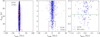 |
Fig. 1 Distance versus time distribution of each close encounter of our sample of stars with β Pic (see Table 1). Left: full sample of 99 416 from the GCNS catalogue. Middle: subset of 1 005 within 6 pc. Right: 116 stars with a closest approach distance dmin < 2 pc. The members of the β PMG are shown in orange. |
3.2 Binary systems
In the previous section, we have treated all the stars as single when propagating their orbits. To account for multiplicity, we searched for companions in the Washington Double Star Catalogue (WDS; Mason et al. 2001), the Multiple Star Catalogue (MSC; Tokovinin 2018), and the wide binary candidate list from El-Badry et al. (2021) based on GEDR3 astrometry. We identified 8 stars among our 49 close encounters as members of 5 binary systems. These cases require further scrutiny to accurately assess their encounter parameters and the possible influence on β Pic. Multiplicity can significantly enhance the perturbative effect – sometimes by more than an order of magnitude – potentially leading to outcomes such as pair disruptions, stellar collisions, or member captures (Li et al. 2020; Torres et al. 2023).
For 4 of the binary systems, full astrometric and RV data are available for both components. One additional companion, GDR3 6377398274119547392 to GDR3 6353376831270492800, lacks RV data. We also added to Table C.1 the companion of GDR3 4078432504018987904, GDR3 4078432297860547072, which as a single star has an empirical probability of less than 87% of encountering β Pic within 2 pc.
For binaries with complete data for both components, we drew stellar masses for each clone from a normal distribution defined by the reported value and its uncertainty, computed the centre-of-mass positions and velocities, and integrated their orbits accordingly. The resulting encounter parameters are listed in Table 3. As with the single-star calculations, the centre-of-mass trajectories confirm the possibility of a close encounter of these systems with β Pic.
Figure 4 shows the distributions of closest-approach distances and times for the final subset, using the centres of mass for the binary systems. As previously noted and visible in Fig. 4, the encounter rate is highest near the present epoch and declines steeply with time (see Sect. 3.3).
3.3 Encounter completeness
We acknowledge that our encounter catalogue (Table C.1) constitutes a lower limit on the true number of close encounters experienced by β Pic. As shown in Table 1, approximately one-third of the stars currently known in the vicinity of β Pic lack RV measurements, making orbital reconstruction for these stars impossible.
Our method identifies encounters by integrating stellar orbits and detecting passages within a critical distance of β Pic. Given the typical relative velocities of the encounters listed in Table C.1, a star can traverse the initial 80 pc sphere around β Pic in just a few megayears or less. Consequently, the number of detected encounters drops sharply when looking further backwards or forwards in time. Beyond 2 Myr, the stellar encounters drop significantly – a trend clearly ∼illustrated in Figs. 1, 2, and 4.
Expanding the search volume by increasing the initial radius would not significantly improve this limitation. For example, of the 49 high-confidence encounters listed in Table C.1, only 7 are presently located at distances greater than 50 pc from β Pic, and all but one of these occurred outside the 0.5 Myr interval. However, the stars currently located further±away would yield less accurate encounters because of the limitations of Gaia data.
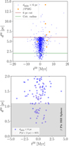 |
Fig. 2 Top: medians of the distance versus time distributions for the 1 005 candidate encounters with β Pic that had dmin < 6 pc, calculated using the method described in Sect. 3.1. The horizontal red line marks the 6 pc limit used to select these sources based on their dmin values (middle panel of Fig. 1). Distributions with d50 values above this line correspond to the 47 more distant, higher-dispersion encounters. The horizontal green line denotes the 2 pc critical radius. The orange points indicate the β PMG members. Bottom: same but for the 96 sources with d50 < 2 pc. The Hill sphere of β Pic is highlighted in grey. Only 49 stars have at least a 95% empirical probability of passing within 2 pc of β Pic and are considered actual encounters (highlighted in pink). |
3.3.1 Expected encounter rates from stellar density
To quantify the completeness of our encounter catalogue, we estimated the expected number of stellar encounters for different spectral types, accounting for their distinct kinematics. The expected number of encounters was calculated as the number of stars passing through a cylindrical interaction volume defined by a cross-sectional area  and a length determined by the travel distance tvS.T., where vS.T. is the characteristic encounter velocity for a given spectral type and t is the time interval considered. The expected number of encounters is given by
  . (Binney & Tremaine 2011), where nS.T. is the number density of stars of a given spectral type. The characteristic encounter velocity is defined as
  . (Torres et al. 2019), where vβP, S.T. is the relative velocity of β Pic with respect to the mean for stars of that spectral type, and σvS.T. is the corresponding velocity dispersion. We adopted solar-relative velocities from Mihalas & Binney (1981), transformed into β Pic’s reference frame, and used stellar densities and velocity dispersions from Torres et al. (2019).
If we apply this method over the 3.5 Myr span between the earliest and the latest encounter, we find an expected total of 160 encounters – over five times the number actually identified (49). However, restricting the analysis to the better-sampled ±0.5 Myr interval, we find 30 encounters identified versus 46 expected, indicating a shortfall of ~35%. This incompleteness is consistent with the ~38% of stars in the GCNS sample lacking RVs, suggesting that our encounter recovery rate is broadly in line with the observational limitations.
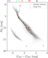 |
Fig. 3 Gaia colour-magnitude Hertzsprung-Russell diagram for the 52 stars that we estimate have a close encounter with β Pic (see Table C.1). The grey field sources were obtained from a Gaia query using magnitude-over-error thresholds matching the lowest-quality values among the encounter sources: parallax>10 mas (maximum distance of 100 pc), parallax_over_error>58, phot_g_mean_flux_over_ error>220, phot_bp_mean_flux_over_error>2.3, and phot_rp_mean_flux_over_error>23.5. Symbols are colour-coded by spectral type. |
3.3.2 The 95% probability threshold
We conducted a self-consistency check to evaluate the impact of our 95% confidence cut. Since we calculated the empirical probability of each star coming within 2 pc of β Pic, summing these probabilities yields the expected number of such close passages over the whole statistical ensemble.
As an example, four stars with probabilities of 2%, 20%, 80%, and 98% contribute a total of two expected encounters. Keeping all four with a low threshold (e.g. 1%) increases completeness but risks false positives; a stricter threshold (e.g. 99%) improves reliability but may exclude real events. The objective is to strike a balance between completeness and robustness, and we therefore adopted a 95% threshold in this work.
By summing only those probabilities above various thresholds, we estimated how many real passages are expected at each confidence level. These results are shown in Fig. 5, alongside the stellar-density-based estimates. We applied this analysis for both the full sample and the ±0.5 Myr interval around the present, where the dataset is more complete.
Overall, our catalogue captures over 40% of the expected close approaches across the full 3.5 Myr, and more than 70% within ±0.5 Myr. Future Gaia data releases are expected to improve this by adding both new sources and better-quality RVs. Currently, RV uncertainties are, on average, ten times larger than those of tangential velocities derived from astrometry, indicating room for improvement in both RV quantity and quality.
Encounter parameters of the centres of mass of the binary systems in which at least one member is among the 49 stars with a 95% empirical probability of having a close encounter with β Pic.
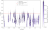 |
Fig. 4 Distance versus time distributions for the 49 encounters with β Pic that have an empirical probability of at least 95% of occurring within 2 pc. The coloured points indicate the rescaled Mahalanobis distances (ensuring a common colour scale for all stars) derived from the encounter parameters. Points above the 95th percentile of this metric are shown in grey. The black bars represent the 95% confidence intervals in time and distance, obtained from the 2.5th and 97.5th percentiles of the corresponding marginal distributions for the further encounters and using the 95th percentile to define the one-tailed distance interval for the closest ones. The central points are the 50th percentiles. The critical radius of 2 pc is indicated by the red horizontal line. The centres of mass of binary systems, listed in Table 3, are marked at the pair [t50, d50] corresponding to that star. |
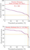 |
Fig. 5 Expected number of stars undergoing a close encounter with β Pic (within 2 pc) as a function of the minimum encounter probability threshold. Top: entire time interval studied (~3.5 Myr). Bottom: most complete portion of the dataset, within the interval ± 0.5 Myr. The orange lines mark the 95% probability threshold adopted±in this work. At this threshold, the expected number of encounters is 49 over 3.5 Myr and 30 in the ±0.5 Myr interval. The red line indicates the independent estimate obtained from the stellar-density-based calculation, yielding 46 encounters in the ±0.5 Myr interval. The total number of expected encounters from our data – corresponding to a 0% probability threshold – is 117 for the full sample and 42 for the ±0.5 Myr interval. |
4 Comparison with Kalas et al. (2001)
The first systematic search for stellar encounters with β Pic was carried out by Kalas et al. (2001), who used astrometric data from the HIPPARCOS catalogue (Perryman et al. 1997) and RVs from Barbier-Brossat & Figon (2000). By propagating linear trajectories for a sample of 21 497 stars, they identified 18 candidates that passed within 5 pc of β Pic over the past 1 Myr. In contrast, our study using Gaia data reveals 146 in the same time span and distance range – nearly an order of magnitude more. This increase reflects both the superior precision and improved completeness of the Gaia dataset. Nonetheless, based on stellar density estimates, that sample is only 50% complete (see Fig. 5).
To directly compare our results with those of Kalas et al. (2001), we computed the 1σ confidence intervals for the time and distance of closest approach using the limits that enclose the 39.35% clones with the lower Mahalanobis distance to the distribution. For the relative velocities at closest approach, we used the 68.27% confidence interval, defined by the 15.87th and the 84.14th percentiles of the marginal velocity distributions. These values are reported in Table 4 for the 17 stars from Kalas et al. (2001) for which Gaia astrometric solutions are available.
One star from the original sample, HIP 93506 (GDR3 6760703042771435136), is absent from our catalogue due to the lack of Gaia astrometry. Additionally, HIP 22122, HIP 31711, HIP 89042, and HIP 114996 are not present in the HIPPARCOS–Gaia crossmatch tables, likely due to low-quality HIPPARCOS astrometric solutions that prevented a robust identification with Gaia. For these objects, we adopted the SIMBAD identification.
Among the 49 encounters listed in Table C.1, only 5 overlap with those from Kalas et al. (2001). It is important to note that Kalas et al. (2001) used a cutoff of 5 pc. They reported 6 stars that have a passage closer than 2 pc with β Pic. Applying our 95% confidence criterion excludes HIP 114996 (GDR3 6492406743706907776), while Kalas et al. (2001) also identified HIP 29958 (GDR3 2993676867708999296) and HIP 38908 (GDR3 5291028181119851776) as having close encounters within 2 pc – cases not supported by our results.
A search in SIMBAD reveals that the Kalas et al. (2001) candidates HIP 19921, HIP 23693, HIP 29568, and HIP 38908 belong to multiple systems. Unresolved multiplicity can distort the astrometry reported in the HIPPARCOS catalogue, likely contributing to inaccuracies in the derived stellar trajectories.
5 Summary and conclusions
We have compiled the most comprehensive catalogue to date of stellar encounters with β Pic by reconstructing the orbits of nearly 100 000 nearby stars using GDR3 astrometry and RV data from Gaia and other major spectroscopic surveys. From this dataset, we identified 49 stars (Table C.1) that either have passed or will pass within 2 pc of β Pic, each with a probability greater than 95%, based on Monte Carlo orbital propagations. Based on stellar density estimates, we assess our sample to be about 65% complete within the time interval ±0.5 Myr. Notably, despite β Pic being the eponym of its famous moving group, none of these encounters involved β PMG members; all were with unrelated field stars.
Among the 49 encounters, we identified 41 single stars and 8 members of 5 binary systems. Four of these systems (WDS J03572-4413, WDS J13237+0243, WDS J05055-5728, and the pair GDR3 4078432504018987904/GDR3 4078432297860547072) seem to have coherent centre-of-mass trajectories, suggesting a genuine close encounter with β Pic. Multiplicity in stellar perturbers can enhance their gravitational influence, highlighting the need for sophisticated dynamical treatments.
Although GDR3 1311454726097258368 passes closest to β Pic (0.442 pc), its relatively low mass (0.07 M⊙) and high velocity (62.16 km s−1) make its perturbation negligible, insufficient to shape the β Pic disc or account for its observed features. The stellar encounters we identify are therefore expected to affect only the distant outskirts of the system; the disc structures revealed by JWST imaging (Rebollido et al. 2024) are more likely the result of internal dynamical processes (e.g. Beust et al. 2024).
This work is limited by the initial data used, particularly the RVs. One-third of our sample near β Pic lacks known RVs, and RV errors are typically ten times larger than those in tangential velocities derived from proper motions and parallaxes. We expect future Gaia data releases to increase the number of stars with available RVs. While planet-hunting RV surveys offer higher accuracy, they are only available for a small subset of stars compared to the Gaia catalogues, and the heterogeneity of sources complicates their systematic use.
Future work should incorporate detailed N-body simulations (that include binary perturbers) and high particle counts; this will allow stronger statistical conclusions to be drawn. The encounter catalogue presented here provides a robust foundation for future dynamical studies of β Pic and, more generally, of how stellar encounters shape the architecture of planetary systems.
Comparison of encounter parameters with those reported by Kalas et al. (2001).
Data availability
The data underlying this article are available on Zen-odo through the following records: sources with RV data within 80 pc of β Pic, the encounter parameters table, the encounter parameters corner plots, and the comparison with Kalas et al. (2001).
Acknowledgements
We thank the referee for their suggestions and comments, which helped us improve the quality and clarity of the paper. JLGM and EV acknowledge the support from the Spanish Ministry of Science and Innovation/State Agency of Research (MCIN/AEI) under the grant PID2021-127289-NB-I00. ST acknowledges the funding from the European Union’s Horizon 2020 research and innovation program under the Marie Skłodowska-Curie grant agreement No. 101034413. AJM acknowledges support from the Swedish National Space Agency (Career Grant 2023-00146) and from the Swedish Research Council (Project Grant 2022-04043). JLGM also sincerely thanks AMP for his careful final reading of this manuscript. This work has made use of data from the European Space Agency (ESA) mission Gaia (https://www.cosmos.esa.int/gaia), processed by the Gaia Data Processing and Analysis Consortium (DPAC). Funding for the DPAC has been provided by national institutions, in particular the institutions participating in the Gaia Multilateral Agreement. We acknowledge the use of the public data products from RAVE (https://www.rave-survey.org), GALAH (https://galah-survey.org), APOGEE ((https://www.sdss.org) and LAMOST (http://www.lamost.org) surveys. This research has also made use of the SIMBAD database and the VizieR catalogue access tool, operated at CDS, Strasbourg, France, as well as the NASA Astrophysics Data System Bibliographic Services and the arXiv pre-print server operated by Cornell University. Computational analyses in this work relied extensively on the NumPy and SciPy libraries for numerical computing, matplotlib and seaborn for data visualization, and the Gala package for Galactic dynamics. This work also made use of Astropy, a community-developed core PYTHON package and an ecosystem of tools and resources for astronomy. We thank the developers and maintainers of these open-source resources for their invaluable contributions to the astronomical community.
References
- Abdurro’uf, Accetta, K., Aerts, C., et al. 2022, ApJS, 259, 35 [NASA ADS] [CrossRef] [Google Scholar]
- Babusiaux, C., Fabricius, C., Khanna, S., et al. 2023, A&A, 674, A32 [NASA ADS] [CrossRef] [EDP Sciences] [Google Scholar]
- Bailer-Jones, C. 2015, A&A, 575, A35 [NASA ADS] [CrossRef] [EDP Sciences] [Google Scholar]
- Bailer-Jones, C. 2018, A&A, 609, A8 [NASA ADS] [CrossRef] [EDP Sciences] [Google Scholar]
- Bailer-Jones, C., Rybizki, J., Andrae, R., & Fouesneau, M. 2018, A&A, 616, A37 [NASA ADS] [CrossRef] [EDP Sciences] [Google Scholar]
- Barbier-Brossat, M., & Figon, P. 2000, A&AS, 142, 217 [NASA ADS] [CrossRef] [EDP Sciences] [Google Scholar]
- Bédard, A., Bergeron, P., & Fontaine, G. 2017, ApJ, 848, 11 [CrossRef] [Google Scholar]
- Beust, H., Lagrange-Henri, A., Vidal-Madjar, A., & Ferlet, R. 1990, A&A, 236, 202 [NASA ADS] [Google Scholar]
- Beust, H., Milli, J., Morbidelli, A., et al. 2024, A&A, 683, A89 [NASA ADS] [CrossRef] [EDP Sciences] [Google Scholar]
- Binney, J., & Tremaine, S. 2011, Galactic Dynamics (Princeton University Press) [Google Scholar]
- Blomme, R., Frémat, Y., Sartoretti, P., et al. 2023, A&A, 674, A7 [NASA ADS] [CrossRef] [EDP Sciences] [Google Scholar]
- Bonavita, M., Fontanive, C., Desidera, S., et al. 2020, MNRAS, 494, 3481 [NASA ADS] [CrossRef] [Google Scholar]
- Brasser, R., & Morbidelli, A. 2013, Icarus, 225, 40 [Google Scholar]
- Brasser, R., Duncan, M., & Levison, H. 2008, Icarus, 196, 274 [Google Scholar]
- Buder, S., Kos, J., Wang, X. E., et al. 2025, PASA, 42, e051 [Google Scholar]
- Cantat-Gaudin, T., & Brandt, T. D. 2021, A&A, 649, A124 [NASA ADS] [CrossRef] [EDP Sciences] [Google Scholar]
- Cataldi, G., Brandeker, A., Wu, Y., et al. 2018, ApJ, 861, 72 [NASA ADS] [CrossRef] [Google Scholar]
- Chen, C. H., Lu, C. X., Worthen, K., et al. 2024, ApJ, 973, 139 [Google Scholar]
- Couture, D., Gagné, J., & Doyon, R. 2023, ApJ, 946, 6 [NASA ADS] [CrossRef] [Google Scholar]
- Darragh-Ford, E., Hunt, J. A. S., Price-Whelan, A. M., & Johnston, K. V. 2023, ApJ, 955, 74 [NASA ADS] [CrossRef] [Google Scholar]
- Deng, L.-C., Newberg, H. J., Liu, C., et al. 2012, RAA, 12, 735 [Google Scholar]
- Dent, W. R., Wyatt, M., Roberge, A., et al. 2014, Science, 343, 1490 [NASA ADS] [CrossRef] [Google Scholar]
- Dones, L., Weissman, P. R., Levison, H. F., & Duncan, M. J. 2004, Star Formation in the Interstellar Medium: In Honor of David Hollenbach, 323, 371 [Google Scholar]
- Dybczyński, P. A. 1994, Celest. Mech. Dyn. Astron., 58, 139 [Google Scholar]
- Eilers, A.-C., Hogg, D. W., Rix, H.-W., & Ness, M. K. 2019, ApJ, 871, 120 [Google Scholar]
- El-Badry, K., Rix, H.-W., & Heintz, T. M. 2021, MNRAS, 506, 2269 [NASA ADS] [CrossRef] [Google Scholar]
- Ferlet, R., Hobbs, L., & Vidal-Madjar, A. 1987, A&A, 185, 267 [NASA ADS] [Google Scholar]
- Forest, E., & Ruth, R. D. 1990, Phys. D: Nonlinear Phenom., 43, 105 [Google Scholar]
- Fouchard, M., Froeschlé, C., Valsecchi, G., & Rickman, H. 2006, Celest. Mech. Dyn. Astron., 95, 299 [NASA ADS] [CrossRef] [Google Scholar]
- Gaia Collaboration (Brown, A. G. A., et al.) 2016a, A&A, 595, A2 [NASA ADS] [CrossRef] [EDP Sciences] [Google Scholar]
- Gaia Collaboration (Prusti, T., et al.) 2016b, A&A, 595, A1 [NASA ADS] [CrossRef] [EDP Sciences] [Google Scholar]
- Gaia Collaboration (Brown, A. G. A., et al.) 2018, A&A, 616, A1 [NASA ADS] [CrossRef] [EDP Sciences] [Google Scholar]
- Gaia Collaboration (Brown, A. G. A., et al.) 2021a, A&A, 649, A1 [NASA ADS] [CrossRef] [EDP Sciences] [Google Scholar]
- Gaia Collaboration, (Smart, R. L., et al.) 2021b, A&A, 649, A6 [Google Scholar]
- Gaia Collaboration (Vallenari, A., et al.) 2023, A&A, 674, A1 [NASA ADS] [CrossRef] [EDP Sciences] [Google Scholar]
- García-Sánchez, J., Preston, R. A., Jones, D. L., et al. 1999, AJ, 117, 1042 [Google Scholar]
- Gianninas, A., Curd, B., Thorstensen, J. R., et al. 2015, MNRAS, 449, 3966 [Google Scholar]
- Golimowski, D. A., Ardila, D. R., Krist, J., et al. 2006, AJ, 131, 3109 [NASA ADS] [CrossRef] [Google Scholar]
- Gosset, E., Damerdji, Y., Morel, T., et al. 2025, A&A, 693, A124 [NASA ADS] [CrossRef] [EDP Sciences] [Google Scholar]
- GRAVITY Collaboration (Abuter, R., et al.) 2021, A&A, 647, A59 [NASA ADS] [CrossRef] [EDP Sciences] [Google Scholar]
- Gray, R. O., Corbally, C. J., Garrison, R. F., et al. 2006, AJ, 132, 161 [Google Scholar]
- Halbwachs, Jean-Louis, Pourbaix, Dimitri, Arenou, Frédéric, et al. 2023, A&A, 674, A9 [NASA ADS] [CrossRef] [EDP Sciences] [Google Scholar]
- Heap, S. R., Lindler, D. J., Lanz, T. M., et al. 2000, ApJ, 539, 435 [Google Scholar]
- Hoeijmakers, H. J., Jaworska, K. P., & Prinoth, B. 2025, A&A, 700, A239 [NASA ADS] [CrossRef] [EDP Sciences] [Google Scholar]
- Holl, B., Sozzetti, A., Sahlmann, J., et al. 2023, A&A, 674, A10 [NASA ADS] [CrossRef] [EDP Sciences] [Google Scholar]
- Hunt, J. A. S., Price-Whelan, A. M., Johnston, K. V., & Darragh-Ford, E. 2022, MNRAS, 516, L7 [NASA ADS] [CrossRef] [Google Scholar]
- Jiménez-Esteban, F. M., Torres, S., Rebassa-Mansergas, A., et al. 2023, MNRAS, 518, 5106 [Google Scholar]
- Kaib, N. A., & Quinn, T. 2008, Icarus, 197, 221 [NASA ADS] [CrossRef] [Google Scholar]
- Kalas, P., Deltorn, J.-M., & Larwood, J. 2001, ApJ, 553, 410 [Google Scholar]
- Katz, D., Sartoretti, P., Guerrier, A., et al. 2023, A&A, 674, A5 [NASA ADS] [CrossRef] [EDP Sciences] [Google Scholar]
- Kiefer, F., Des Etangs, A. L., Boissier, J., et al. 2014, Nature, 514, 462 [NASA ADS] [CrossRef] [Google Scholar]
- Kilic, M., Bergeron, P., Kosakowski, A., et al. 2020, ApJ, 898, 84 [Google Scholar]
- Lacour, S., Wang, J., Rodet, L., et al. 2021, A&A, 654, L2 [NASA ADS] [CrossRef] [EDP Sciences] [Google Scholar]
- Lagrange, A., Vidal-Madjar, A., Deleuil, M., et al. 1995, A&A, 296, 499 [Google Scholar]
- Lagrange, A.-M., Gratadour, D., Chauvin, G., et al. 2009a, A&A, 493, L21 [NASA ADS] [CrossRef] [EDP Sciences] [Google Scholar]
- Lagrange, A.-M., Kasper, M., Boccaletti, A., et al. 2009b, A&A, 506, 927 [NASA ADS] [CrossRef] [EDP Sciences] [Google Scholar]
- Lagrange, A.-M., Bonnefoy, M., Chauvin, G., et al. 2010, Science, 329, 57 [Google Scholar]
- Lagrange, A.-M., Boccaletti, A., Milli, J., et al. 2012, A&A, 542, A40 [NASA ADS] [CrossRef] [EDP Sciences] [Google Scholar]
- Lagrange, A.-M., Meunier, N., Rubini, P., et al. 2019, Nat. Astron., 3, 1135 [NASA ADS] [CrossRef] [Google Scholar]
- Lecavelier des Etangs, A., Cros, L., Hébrard, G., et al. 2022, Sci. Rep., 12, 5855 [NASA ADS] [CrossRef] [Google Scholar]
- Lee, J., & Song, I. 2024, ApJ, 967, 113 [Google Scholar]
- Lee, R. A., Gaidos, E., van Saders, J., Feiden, G. A., & Gagné, J. 2024, MNRAS, 528, 4760 [NASA ADS] [CrossRef] [Google Scholar]
- Levison, H. F., Morbidelli, A., & Dones, L. 2004, AJ, 128, 2553 [Google Scholar]
- Li, D., Mustill, A. J., & Davies, M. B. 2020, MNRAS, 499, 1212 [Google Scholar]
- Liebing, F., Jeffers, S. V., Zechmeister, M., & Reiners, A. 2023, A&A, 673, A43 [NASA ADS] [CrossRef] [EDP Sciences] [Google Scholar]
- Lindegren, L., & Dravins, D.. 2003, A&A, 401, 1185 [NASA ADS] [CrossRef] [EDP Sciences] [Google Scholar]
- Lindegren, L., Bastian, U., Biermann, M., et al. 2021a, A&A, 649, A4 [EDP Sciences] [Google Scholar]
- Lindegren, L., Klioner, S. A., Hernández, J., et al. 2021b, A&A, 649, A2 [EDP Sciences] [Google Scholar]
- Liu, C., Fu, J., Shi, J., et al. 2020, RAA, submitted [arXiv:2005.07210] [Google Scholar]
- Luhman, K. L. 2024, AJ, 168, 159 [NASA ADS] [CrossRef] [Google Scholar]
- Luo, A.-L., Zhao, Y.-H., Zhao, G., et al. 2015, RAA, 15, 1095 [NASA ADS] [Google Scholar]
- Maíz Apellániz, J. 2022, A&A, 657, A130 [NASA ADS] [CrossRef] [EDP Sciences] [Google Scholar]
- Mason, B. D., Wycoff, G. L., Hartkopf, W. I., Douglass, G. G., & Worley, C. E. 2001, AJ, 122, 3466 [Google Scholar]
- Matrà, L., Wyatt, M. C., Wilner, D. J., et al. 2019, AJ, 157, 135 [CrossRef] [Google Scholar]
- Mihalas, D., & Binney, J. 1981, Galactic Astronomy. Structure and Kinematics (San Francisco: Freeman) [Google Scholar]
- Morbidelli, A. 2005, arXiv preprint [arXiv:astro-ph/0512256] [Google Scholar]
- Mouillet, D., Larwood, J. D., Papaloizou, J. C. B., & Lagrange, A. M. 1997, MNRAS, 292, 896 [Google Scholar]
- Nesvornỳ, D. 2018, ARA&A, 56, 137 [CrossRef] [Google Scholar]
- Nowak, M., Lacour, S., Lagrange, A.-M., et al. 2020, A&A, 642, L2 [NASA ADS] [CrossRef] [EDP Sciences] [Google Scholar]
- Oort, J. 1950, BAN, 11, 91 [NASA ADS] [Google Scholar]
- Paegert, M., Stassun, K. G., Collins, K. A., et al. 2021, arXiv e-prints [arXiv:2108.04778] [Google Scholar]
- Pecaut, M. J., & Mamajek, E. E. 2013, ApJS, 208, 9 [Google Scholar]
- Perryman, M. A., Lindegren, L., Kovalevsky, J., et al. 1997, A&A, 323, L49 [NASA ADS] [Google Scholar]
- Portegies Zwart, S., Torres, S., Cai, M. X., & Brown, A. G. A. 2021, A&A, 652, A144 [NASA ADS] [CrossRef] [EDP Sciences] [Google Scholar]
- Price-Whelan, A. M. 2017, JOSS, 2, 18 [Google Scholar]
- Price-Whelan, A., Sipőcz, B., Lenz, D., et al. 2020, https://doi.org/10.5281/zenodo.4159870 [Google Scholar]
- Rebollido, I., Stark, C. C., Kammerer, J., et al. 2024, AJ, 167, 69 [NASA ADS] [CrossRef] [Google Scholar]
- Reid, M. J., & Brunthaler, A. 2004, ApJ, 616, 872 [Google Scholar]
- Rickman, H. 1976, Bull. Astron. Inst. Czechosl., 27, 92 [Google Scholar]
- Shannon, A., Jackson, A. P., & Wyatt, M. C. 2019, MNRAS, 485, 5511 [CrossRef] [Google Scholar]
- Smith, B. A., & Terrile, R. J. 1984, Science, 226, 1421 [Google Scholar]
- Steinmetz, M., Matijevič, G., Enke, H., et al. 2020, AJ, 160, 82 [NASA ADS] [CrossRef] [Google Scholar]
- Taylor, M. B. 2005, in Astronomical Society of the Pacific Conference Series, 347, Astronomical Data Analysis Software and Systems XIV, eds. P. Shopbell, M. Britton, & R. Ebert, 29 [Google Scholar]
- Thébault, P., & Beust, H. 2001, A&A, 376, 621 [Google Scholar]
- Tobin, W., Barnes, S. I., Persson, S., & Pollard, K. R. 2019, MNRAS, 489, 574 [NASA ADS] [CrossRef] [Google Scholar]
- Tokovinin, A. 2018, ApJS, 235, 6 [NASA ADS] [CrossRef] [Google Scholar]
- Torres, S., Cai, M. X., Brown, A., & Zwart, S. P. 2019, A&A, 629, A139 [NASA ADS] [CrossRef] [EDP Sciences] [Google Scholar]
- Torres, S., Naoz, S., Li, G., & Rose, S. C. 2023, MNRAS, 524, 1025 [Google Scholar]
- Tsantaki, M., Pancino, E., Marrese, P., et al. 2022, A&A, 659, A95 [NASA ADS] [CrossRef] [EDP Sciences] [Google Scholar]
- Vincent, O., Barstow, M. A., Jordan, S., et al. 2024, A&A, 682, A5 [NASA ADS] [CrossRef] [EDP Sciences] [Google Scholar]
- Vokrouhlický, D., Nesvornỳ, D., & Dones, L. 2019, AJ, 157, 181 [CrossRef] [Google Scholar]
- Wenger, M., Ochsenbein, F., Egret, D., et al. 2000, A&AS, 143, 9 [NASA ADS] [CrossRef] [EDP Sciences] [Google Scholar]
- Zuckerman, B., Song, I., Bessell, M. S., & Webb, R. A. 2001, ApJ, 562, L87 [NASA ADS] [CrossRef] [Google Scholar]
Appendix A TOPCAT queries
To select the sphere around β Pic, we used the heliocentric positions of each star, r⋆, and β Pic, rβP, to check whether the distance is less than 80 pc, ((r⋆ − rβP)2 < (80 pc)2):
dotProduct(subtract(astromXYZ(RA_ICRS, DE_ICRS, Plx), astromXYZ(BP_RA, BP_DEC, BP_Plx)), subtract(astromXYZ(RA_ICRS, DE_ICRS, Plx), astromXYZ(BP_RA, BP_DEC, BP_Plx))) < 80*80
Here the function astromXYZ calculates the Cartesian components of the position in parsecs from right ascension and declination (in degrees) and parallax (in milliarcseconds) and BP_RA = 86.8212345201 deg, BP_DEC = −51.0661362578 deg and BP_Plx = 86.8212345201 mas, the coordinates of β Pic.
To select GDR3 RV data over GCNS, we used the error value as an indicator of data availability:
| RV_o = eRV_dr3 > 0 ? RV_dr3 : RV_GCNS | # Radial velocity |
| eRV_o = eRV_dr3 > 0 ? eRV_dr3 : eRV_GCNS | # Radial velocity uncertainty |
| r_RV_o = eRV_dr3 > 0 ? "GDR3" : r_RV_GCNS | # Radial velocity reference |
To select the data from the survey with the smallest error:
| RV_o = (eRV_i < eRV_a) | !(eRV_a > 0) ? RV_i : RV_a |
| eRV_o = (eRV_i < eRV_a) | !(eRV_a > 0) ? eRV_i : eRV_a |
| r_RV_o = (eRV_i < eRV_a) | !(eRV_a > 0) ? r_RV_i : "ALTERNATIVE_SURVEY_NAME" |
Here, the subscript ‘_i’ refers to the input survey, ‘_a’ to the alternative survey whose error is being compared, and ‘_o’ to the resulting parameters.
Appendix B Clone set example
This appendix presents an example outcome of the orbital integrations: the clone distribution of relative positions, velocities, and encounter times for GDR3 5038817840251308288 with β Pic. The corresponding corner plot is shown in Fig. B.1. Corner plots for the remaining high-confidence encounters, as well as for the centres of mass of the binary systems, are available at Zenodo.
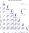 |
Fig. B.1 Encounter parameters (X, Y, Z, U, V, W, t) of the clones of GDR3 5038817840251308288 relative to β Pic. The 50% most clustered clones, selected using the Mahalanobis distance, are highlighted. The values above the histograms indicate the median (x50) and the 95% confidence interval [x2.5, x97.5]. |
Appendix C Encounter parameter table
Encounter parameters of the 49 stars with a 95% empirical probability of having a close encounter with β Pic (d < 2 pc), or their companions, treating all sources as single.
All Tables
Encounter parameters of the centres of mass of the binary systems in which at least one member is among the 49 stars with a 95% empirical probability of having a close encounter with β Pic.
Encounter parameters of the 49 stars with a 95% empirical probability of having a close encounter with β Pic (d < 2 pc), or their companions, treating all sources as single.
All Figures
|
Fig. 1 Distance versus time distribution of each close encounter of our sample of stars with β Pic (see Table 1). Left: full sample of 99 416 from the GCNS catalogue. Middle: subset of 1 005 within 6 pc. Right: 116 stars with a closest approach distance dmin < 2 pc. The members of the β PMG are shown in orange. |
| In the text | |
|
Fig. 2 Top: medians of the distance versus time distributions for the 1 005 candidate encounters with β Pic that had dmin < 6 pc, calculated using the method described in Sect. 3.1. The horizontal red line marks the 6 pc limit used to select these sources based on their dmin values (middle panel of Fig. 1). Distributions with d50 values above this line correspond to the 47 more distant, higher-dispersion encounters. The horizontal green line denotes the 2 pc critical radius. The orange points indicate the β PMG members. Bottom: same but for the 96 sources with d50 < 2 pc. The Hill sphere of β Pic is highlighted in grey. Only 49 stars have at least a 95% empirical probability of passing within 2 pc of β Pic and are considered actual encounters (highlighted in pink). |
| In the text | |
|
Fig. 3 Gaia colour-magnitude Hertzsprung-Russell diagram for the 52 stars that we estimate have a close encounter with β Pic (see Table C.1). The grey field sources were obtained from a Gaia query using magnitude-over-error thresholds matching the lowest-quality values among the encounter sources: parallax>10 mas (maximum distance of 100 pc), parallax_over_error>58, phot_g_mean_flux_over_ error>220, phot_bp_mean_flux_over_error>2.3, and phot_rp_mean_flux_over_error>23.5. Symbols are colour-coded by spectral type. |
| In the text | |
|
Fig. 4 Distance versus time distributions for the 49 encounters with β Pic that have an empirical probability of at least 95% of occurring within 2 pc. The coloured points indicate the rescaled Mahalanobis distances (ensuring a common colour scale for all stars) derived from the encounter parameters. Points above the 95th percentile of this metric are shown in grey. The black bars represent the 95% confidence intervals in time and distance, obtained from the 2.5th and 97.5th percentiles of the corresponding marginal distributions for the further encounters and using the 95th percentile to define the one-tailed distance interval for the closest ones. The central points are the 50th percentiles. The critical radius of 2 pc is indicated by the red horizontal line. The centres of mass of binary systems, listed in Table 3, are marked at the pair [t50, d50] corresponding to that star. |
| In the text | |
|
Fig. 5 Expected number of stars undergoing a close encounter with β Pic (within 2 pc) as a function of the minimum encounter probability threshold. Top: entire time interval studied (~3.5 Myr). Bottom: most complete portion of the dataset, within the interval ± 0.5 Myr. The orange lines mark the 95% probability threshold adopted±in this work. At this threshold, the expected number of encounters is 49 over 3.5 Myr and 30 in the ±0.5 Myr interval. The red line indicates the independent estimate obtained from the stellar-density-based calculation, yielding 46 encounters in the ±0.5 Myr interval. The total number of expected encounters from our data – corresponding to a 0% probability threshold – is 117 for the full sample and 42 for the ±0.5 Myr interval. |
| In the text | |
|
Fig. B.1 Encounter parameters (X, Y, Z, U, V, W, t) of the clones of GDR3 5038817840251308288 relative to β Pic. The 50% most clustered clones, selected using the Mahalanobis distance, are highlighted. The values above the histograms indicate the median (x50) and the 95% confidence interval [x2.5, x97.5]. |
| In the text | |
Current usage metrics show cumulative count of Article Views (full-text article views including HTML views, PDF and ePub downloads, according to the available data) and Abstracts Views on Vision4Press platform.
Data correspond to usage on the plateform after 2015. The current usage metrics is available 48-96 hours after online publication and is updated daily on week days.
Initial download of the metrics may take a while.