| Issue |
A&A
Volume 704, December 2025
|
|
|---|---|---|
| Article Number | A292 | |
| Number of page(s) | 11 | |
| Section | Galactic structure, stellar clusters and populations | |
| DOI | https://doi.org/10.1051/0004-6361/202555965 | |
| Published online | 22 December 2025 | |
Kinematic, elemental, and structural dependences on metallicity in the Galactic bulge
School of Astronomy and Space Sciences, University of Chinese Academy of Sciences,
Beijing
100049,
PR China
★ Corresponding author: This email address is being protected from spambots. You need JavaScript enabled to view it.
Received:
16
June
2025
Accepted:
22
October
2025
Abstract
Context. The Galactic bulge is known to have multiple stellar populations according to the metallicity-distribution-function (MDF) peaks. These populations show varying properties of kinematic, elemental, and spatial distributions.
Aims. This study aims to investigate metallicity-dependent variations in the kinematic properties, elemental abundances, and spatial distributions of Galactic-bulge stars and distinguishes these populations.
Methods. We selected bulge stars from APOGEE DR17 cross-matched with astrometric data from Gaia DR3. Bulge stars were divided into subsamples with the line-of-sight velocity dispersion analyzed, and the peaks of MDF were detected by both Gaussian mixture models (GMMs) and scipy.signal.find_peaks. Orbital parameters (e.g., actions) were calculated via orbital integration, and the kinematic dependence on metallicity was investigated. A GMM was also conducted to kinematically distinguish the metal-poor and metal-rich populations. Analyses were carried out of the bulge stars (including retrograde stars), their elemental abundances, and the [Mg/Mn]–[Al/Fe] plane to investigate potential accreted components. Finally, the shapes (X-shaped or boxy) of bulge stars with different metallicities were analyzed through least-squares fitting based on the analytical bulge models.
Results. By studying the kinematic, elemental, and structural dependences on metallicity for bulge stars, our findings are concluded as follows. (1) Six peaks are detected in the bulge MDF, encompassing values reported in previous studies, suggesting a complex composition of bulge populations. (2) An inversion relationship is well observed in metal-rich subsamples, while absent in metal-poor subsamples. (3) Metal-poor populations exhibit larger dispersions than metal-rich stars (which is also revealed by GMM decomposition), suggesting that metal-rich stars are kinematically coherent. (4) Retrograde stars are confined to ∼1 kpc of the Galactic center, with their relative fraction decreasing at higher [Fe/H] – a trend potentially linked to the “spin-up” process of Galactic disks. (5) Metal-rich bulge stars with [Al/Fe] < −0.15 are likely associated with a disk-accreted substructure, while all elemental planes exhibit bimodality, but Na abundances rise monotonically with metallicity. (6) In general, stars with all metallicities support a boxy profile.
Key words: Galaxy: bulge / Galaxy: kinematics and dynamics / Galaxy: structure
© The Authors 2025
 Open Access article, published by EDP Sciences, under the terms of the Creative Commons Attribution License (https://creativecommons.org/licenses/by/4.0), which permits unrestricted use, distribution, and reproduction in any medium, provided the original work is properly cited.
This article is published in open access under the Subscribe to Open model. This email address is being protected from spambots. You need JavaScript enabled to view it. to support open access publication.
1 Introduction
The bulges and bars are commonly found in disk galaxies, with at least ∼45% of disk galaxies exhibiting these features (Lütticke et al. 2000). There are two main types of bulges: classical bulges and pseudo-bulges. The classical bulges are formed through hierarchical mergers (Wyse et al. 1997) with predominant random motions of stars (Fisher & Drory 2016) and they have a surface-brightness profile with Sersic index n > 2 and kinematics similar to elliptical galaxies (Kormendy & Kennicutt 2004; Athanassoula 2005). By contrast, the pseudo-bulges could have formed by disk and bar instabilities on a longer timescale (Combes & Sanders 1981; Wyse et al. 1997) or by a high-redshift starburst (see Okamoto 2013 for an alternative view).
Previous studies have shown that the Galactic bulge is a boxy/peanut (B/P) shaped pseudo-bulge using the red-clump-giant (RCG) star count method (Stanek et al. 1994; Babusiaux & Gilmore 2005; Ness & Lang 2016). An X-shaped component in the bulge at higher latitude is also identified using RCG star counts (McWilliam & Zoccali 2010; Nataf et al. 2010; Wegg & Gerhard 2013) and simulations (Gardner et al. 2014; Li & Shen 2015; Abbott et al. 2017). However, there are arguments that the X-shaped structure could be an artifact, as RCGs do not exhibit a distinct narrow peak in their luminosity function, which is attributed to observational evidence of an X shape in the density (López-Corredoira 2016; López-Corredoira et al. 2019). The morphology of the Galactic bulge is also related to stellar ages and metallicity. Semczuk et al. (2022) used the Auriga simulation to find that younger stars exhibited a more pronounced B/P shape and X-shaped component when projected side-on, compared to older stars. Athanassoula et al. (2017) found that the metal-poor stars form a flattened spheroidal-like component, while the metal-rich stars show a clear X shape when viewed side-on in their simulation.
The presence of multiple stellar populations in the Galactic bulge leads to several peaks in the metallicity distribution function (MDF). The MDF has been studied using various tracers such as RGB, RCG, M giants, and dwarfs (Zoccali et al. 2008; Uttenthaler et al. 2012; Hill et al. 2011; Ness et al. 2013a; Rich et al. 2012; Bensby et al. 2017). Notably, several peaks have been discovered in the metal-poor range (−0.8 < [Fe/H] < 0) in previous studies, while only two peaks were found at ∼0.10 and ∼0.30 in the metal-rich region ([Fe/H] > 0), possibly suggesting a more complex origin of those metal-poor stars and a relatively coherent origin of the metal-rich stars. Using a limited sample of metal-poor stars, Lucey et al. (2019) suggested these stars were neither halo interlopers nor accreted populations, based on their large dispersions in both elemental abundances and α-element enhancement. However, the metal-poor bulge may still keep records about the proto-Galaxy (Rix et al. 2022; Horta & Schiavon 2024) or possible accreted substructures, known as Kraken, Koala, or Heracles (Kruijssen et al. 2020; Forbes 2020; Horta et al. 2021), that are within the inner Galaxy. By contrast, the origin of the metal-rich stars in the bulge has not been thoroughly explored, and the reason why the extremely metal-rich stars are confined within ∼1.5 kpc of the Galactic center remains unclear (Rix et al. 2024).
The kinematic properties of the Galactic bulge also exhibit a strong dependence on metallicity. Along the minor axis of the bulge, metal-poor stars have larger dispersions of radial velocity and line-of-sight velocity than the metal-rich stars at |b| > 4°, as revealed by giant stars (Rich 1990; Minniti 1996). An inverted trend could also be observed at lower latitudes where the metal-rich stars show bar-like high-velocity dispersions (Babusiaux et al. 2014; Babusiaux 2016). This situation differs from that of the Galactic disk, where metal-rich young-disk stars are less perturbed by the gravitational potential and exhibit lower velocity dispersions (Garzon et al. 2024). Boin et al. (2024) conducted an N-body simulation in which metal-rich stars were placed in a thin disk, while metal-poor stars were assigned to a thick disk. Their simulation demonstrated that metal-rich stars were more easily trapped by bar instability, successfully reproducing the observed trend at low latitudes and suggesting a disk origin for the bulge. This is not surprising, as early studies have indicated the chemical similarities between the local thick disk and the Galactic bulge (Meléndez et al. 2008; Alves-Brito et al. 2010), indicating that the bulge could form from the buckling instability of the bar and migration of disk stars (Erwin & Debattista 2016; Lian et al. 2021; Molero et al. 2024). Stellar migration is driven by changes in angular momentum and epicyclic amplitude, processes known as “churning" and “blurring" (e.g., Schönrich & Binney 2009). Across latitudes of |b| < 5°, the metal-poor stars with [Fe/H] < −1 show the slowest rotation and flattest velocity dispersion, while the metal-rich counterparts have the fastest rotation and highest dispersions with 0 < l < 35° (Ness et al. 2016), which suggests a boxy profile of the bulge.
The bimodal distribution of bulge stars in the [Mg/Fe]-[Fe/H] plane was discovered and primarily studied in Rojas-Arriagada et al. (2019), which showed that the stars in the metal-rich and metal-poor modes of the bulge’s MDF represent distinct evolutionary sequences that overlap at super-solar metal-licity. The downward trend of [Mg/Fe] at super-solar metallicity was first observed by Johnson et al. (2014) and Gonzalez et al. (2015), where the knee was between −0.6 and −0.4 metallicity ([Fe/H]) (Friaça & Barbuy 2017; Bensby et al. 2017). The bimodality of other α elements such as O, Si, and Ca (which also includes [C/N] abundances) was also observed in Queiroz et al. (2021), suggesting a discontinuous star formation path. For an iron-peak element such as Mn, [Mn/Fe] exhibits an upward trend with increasing [Fe/H] (McWilliam et al. 2003; Barbuy et al. 2013; Schultheis et al. 2017), which is consistent with the chemical-evolution model in the solar neighborhood with asymptotic-giant-branch (AGB) stars and super-AGB stars included (Kobayashi et al. 2020). Furthermore, the [Mn/O]– [Fe/H] distribution for the bulge stars overlaps with those of thick- and thin-disk stars (Barbuy et al. 2013), suggesting that its evolutionary paths may resemble both disks, potentially explaining the α-element bimodality or indicating a possible disk origin for some bulge stars. Regarding the odd-z elements Al and Na, Al abundances behave as an α element, exhibiting a bimodal pattern in both observations (McWilliam 2016) and chemical-evolution models (Kobayashi et al. 2006). In contrast, the decreasing trend of Na at higher metallicity was not well predicted by Kobayashi et al. (2006).
The kinematics, chemical distributions, and structural characteristics of different populations in the Galactic bulge may differ significantly, as indicated above, suggesting distinct origins and evolutionary paths for stars of varying metallicities. Therefore, we studied the kinematic, elemental, and structural dependences on metallicity in the Galactic bulge to explore the underlying properties that have not been fully diagnosed before. For kinematics of bulge stars, we included the actions (i.e., Jr, Jz, and Jϕ) that could provide deeper dynamical insights as they are integrals of motion under a symmetric gravitational potential. This paper is structured as follows. Section 2 gives a brief introduction to the data selection and derivation of orbital parameters. The results are presented in Section 3. The discussion and summary are given in Section 4.
2 Data
In this work, we used the elemental abundances from the Apache Point Observatory Galactic Evolution Experiment (APOGEE) data release 17 (Abdurro’uf et al. 2022) and proper motions and positions from Gaia data release 3 (Gaia Collaboration 2016, 2023). We applied the following cuts for data quality: EXTRATARG = 0; SNR> 70; log g < 3.6 dex; 3500 < TEFF < 5500 K; VERR < 10 km/s; FE_H_FLAG = 0; [Fe/H] > −0.8; dist_error/dist < 0.2. The first five conditions were used to select giant stars with high signal-to-noise ratios, precise heliocentric velocities, and accurate metallicity estimates. The metallicity cut was used to remove the major contamination from Galactic stellar-halo interlopers (Feuillet et al. 2022). Studies have used the apocenter radius Rap > 3.5 kpc (Han et al. 2025) to remove possible interlopers. The threshold proposed by Lucey et al. (2022) could exclude the interlopers from the metal-weak thick disk (MWTD). The percentages of stars with Rap < 3.5 kpc and Rap < 6 kpc in the subsequent bulge sample are 73.2% and 98.2%, respectively. Yan et al. (2022) revealed that MWTD only contributed significantly when [Fe/H] < −0.8 in the inner region. Therefore, our sample contains negligible fraction from MWTD interlopers. Besides, interlopers from the inner stellar halo usually have Rap ≳ 6 kpc (e.g., Deason et al. 2018); thus, the sample contains negligible interlopers from the MWTD and halo by this metallicity cut. Since only ∼5% stars with [Fe/H] < − 1 are in the Galactic bulge, this selection does not affect the general study of bulge populations (Ness & Freeman 2016). The last condition is to constrain the precision of distances, which are taken from the astroNN value-added catalog (Leung & Bovy 2019). The astroNN neural network incorporates Ks extinctions, assuming no uncertainty in the extinction correction due to the high precision of APOGEE stellar extinction estimates. Moreover, extinction could alternatively be inferred jointly from the spectra and multiband photometry, so the distances for bulge stars are reliable.
For the selection of bulge stars, we required a cylindrical radius of R < 3.5 kpc (Ness et al. 2013b) and |z| < 1 kpc, resulting in a total sample of 7156 stars. It should be noted that we do not impose any additional quality cuts when analyzing kinematics and spatial distributions of the bulge stars to maintain a slightly larger sample size. However, for the analysis of elemental abundances, we required that ASPCAPFLAG = 0 to ensure the abundances quality, which resulted in a sample of 5772 stars.
For the derivation of orbital parameters, we integrated the orbits backward over a period of 5 Gyr using the galpy package (Bovy 2015). Here, the Local Standard of Rest (LSR) velocity VLSR is 232 km/s and the cylindrical distance of the Sun is 8.21 kpc (McMillan 2017). The peculiar motion of the Sun is [U⊙, V⊙, W⊙] = [11.1, 12.24, 7.25] km/s (Schönrich et al. 2010), and the Sun is located at 20.8 pc above the Galactic mid-plane (Bennett & Bovy 2019). We adopted the axisymmetric gravitational potential MWPotential2014 (Bovy 2015) to obtain the conserved quantities: the radial action, Jr, the vertical action, Jz, the azimuthal action, Jϕ (which is equal to Lz), and other orbital parameters such as eccentricity (e) and the maximum height above the mid-plane (Zmax). The potential adopted here includes a spherical bulge and dark-matter halo and a Miyamoto–Nagai disk (see detailed parameters in Table 1 of Bovy 2015). We also calculated the circularity (η) of the orbits, which is defined as |Lz|/Lc(E), where Lc(E) is the angular momentum with given energy (E).
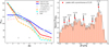 |
Fig. 1 Left panel: line-of-sight velocity dispersions (in units of km/s) across 0 < |b| < 10° along the minor axis (|l| < 2°) of the bulge. The solid red and blue lines represent metal-rich and metal-poor stars, respectively. The dashed lines represent the metal-rich and metal-poor subsamples, while the black cross indicates EMR stars. Right panel: MDF of bulge. Six peaks have been identified with a prominence of 0.25, as indicated by the black arrows. |
3 Results
3.1 Line-of-sight velocity dispersions and MDF of the Galactic bulge
In this work, we defined metal-rich stars with [Fe/H] > 0 and metal-poor stars with −0.8 < [Fe/H] < 0 in later analyses. We divided the metal-poor and metal-rich stars into two subsamples: −0.8 < [Fe/H] < −0.4 and −0.4 < [Fe/H] < 0 for metal-poor stars; 0 < [Fe/H] < 0.3 and [Fe/H] > 0.3 for metal-rich stars. We also adopted the definition of extremely metal-rich (EMR) stars with [Fe/H] > 0.45 in Rix et al. (2024). We calculated the dispersions of line-of-sight velocity along the minor axis (|l| < 2°) of the bulge in five |b| bins within the 0< |b| < 10° range. As shown in the left panel of Figure 1, the metal-poor stars have larger line-of-sight velocity dispersions than metal-rich stars when |b| ≳ 3°, which is in good agreement with previous studies (Babusiaux et al. 2010, 2014; Ness et al. 2013b; Rojas-Arriagada et al. 2014).
It is also observed that the metal-rich subsamples exhibit an inverted trend at higher latitude |b| 6.5°. The two metal-rich subsamples exhibit similar dispersions, suggesting that they may be drawn from a single distribution. The p values from the Kolmogorov–Smirnov test and F test are 1.000 and 0.551, respectively, failing to reject the null hypothesis. This suggests that the two subsamples likely originate from the same distribution. However, this result is expected, given that the metal-rich stars exhibit a peak around 0.3 (as seen in the later MDF analysis). Using this 0.3 threshold to divide the subsamples inevitably leads to significant overlap in their distributions. However, the inverted trend does not strictly hold for the metal-poor subsamples, as stars with −0.8 < [Fe/H] < − 0.4 still have larger dispersions than those with −0.4 < [Fe/H] < 0 at |b| ≲ 3°. A similar pattern observed in metal-poor stars is also presented in Khoperskov et al. (2025), which used an orbit-superposition approach. However, in their analysis, stars with −1.0 < [Fe/H] < −0.5 exhibited larger dispersions than those with −0.5 < [Fe/H] < 0, nearly across all regions with |b| < 15°. The dispersion differences suggest that the metal-poor and metal-rich stars have a distinct origin. In the N-body simulation of Boin et al. (2024), the metal-poor stars ([Fe/H] < −0.5) and metal-intermediate stars (−0.5 < [Fe/H] < 0) still exhibit the inverted trend at low latitudes. This indicates that the metal-poor stars origin from the thick disk and the metal-rich stars from the thin disk cannot fully account for the observations. Interestingly, EMR stars have very low line-of-sight velocity dispersions of ∼60 km/s (only 2 bins for 2 < |b| < 6° due to the small sample size), which indicates that EMR stars have more coherent kinematics or a nearly zero mean line-of-sight velocity in the inner bulge (see Figure 5 of Rix et al. 2024).
The peaks of MDF in the Galactic bulge were identified by adopting a scipy.signal.find_peaks function and Gaussian mixture model (GMM), respectively. The scipy.signal.find_peaks function successfully identified six peaks in the MDF with a prominence of 0.25, which are close to those reported in previous studies using RGB stars and red-clump (RC) stars. We applied the GMM by minimizing the Bayesian-information-criterion (BIC) value to find the optimal number of Gaussian components. Six components were also identified by the GMM, although there are slight shifts in the resulting values. It is worth emphasizing that the results of the GMM may lack statistical significance, as its prior assumption that each component follows a Gaussian distribution is unfavorable for potentially skewed distributions. However, the MDF of the sample shows no significant tail, making the use of a GMM a valid simplification. Moreover, the discovered peaks are similar, indicating that these components are securely fit. The validity of the GMM for unbiased distributions is further supported by previous studies such as Ness et al. (2013a) and Zoccali et al. (2018).
From Table 1, the metal-rich peak at ∼0.3 is the easiest to identify among previous studies, as it has the highest prominence of ∼1.20, while the metal-rich peak at 0.15 only has a prominence of ∼0.31. Metal-poor stars generally exhibit multiple peaks, whereas metal-rich stars typically exhibit only one or two peaks. This suggests that metal-poor stars have more complex origins, while metal-rich stars may share a common origin. As suggested by Matteucci et al. (2019), metal-rich populations may originate from the inner disk due to the secular evolution of the bar, while metal-poor populations could be linked to the chemically complex inner and outer bulge regions (Lucey et al. 2022).
In Table 1, most studies indicate a metal-rich peak around 0.3 (Zoccali et al. 2008, 2018; Uttenthaler et al. 2012; Schultheis et al. 2017; Wylie et al. 2021) and 0.32 for Hill et al. (2011), as well as the values of 0.33 and 0.36 obtained in this work. It is worth noting that a less metal-rich peak was detected by both Ness et al. (2013a) (0.13) and this work (0.15 and 0.16). Bensby et al. (2013) and Bensby et al. (2017) used a microlensed dwarf and detected a peak at [Fe/H] ∼ 0.08 and ∼0.12, respectively. Ness et al. (2013a) attributed the peak to the instability-driven bar/bulge formation from the thin disk, and it is more prominent at a lower latitude (|b| = −5°). Since ∼71% of the have |b| ≲ °, is sample 5 it reasonable that this peak is detected. Regarding the peak at −0.11/ − 0.08 in this work, a similar feature was only detected in Gonzalez et al. (2011), where the median [Fe/H] ratio in the field (+5, –3) was −0.08. However, since no other studies have confirmed this result, the peak may be spurious. As for the three metal-poor peaks detected in this work, they exhibit values consistent with those reported in previous studies. For the possible contamination from disk stars here, Rojas-Arriagada et al. (2020) found that a spatial limit of R = 3.5 kpc could well separate the rotation-supported disk and bar+pressure-supported bulge kinematically. Moreover, Boin et al. (2024) selected bulge stars in a spatial way to analyze the bugle kinematics. Their results were consistent with previous studies and their simulation. Therefore, the disk contamination does not have a crucial affect on the analysis.
Comparisons between peaks of MDF from this study and those from previous literature, where the parentheses indicate the
3.2 Kinematic dependence on metallicity in the Galactic bulge
Figure 2 illustrates the kinematic dependence on metallicity in terms of actions (Jr, Jz, and Jϕ), e, Zmax, and circularity, η. The trends of e, Zmax, and η with respect to metallicity are similar to those of actions (Jr, Jz, and Jϕ), as they are corresponding physical quantities. From the middle column of Figure 2, we can see that there is a downward trend of Jz with increasing metal-licity, indicating that metal-rich stars are vertically colder than metal-poor stars, allowing them to be more easily centered in the mid-plane (also see Ness et al. 2016). Interestingly, Jr (corresponding to e) exhibits a downward trend in the metal-poor range (−0.8 < [Fe/H] < 0) and an upward trend in the metal-rich range ([Fe/H] > 0). Additionally, there is a clear inverse trend in the Jϕ – [Fe/H] plane. The more metal-poor stars are typically older and experienced more gravitational perturbation, thus leading to higher vertical velocity dispersions (i.e., Jz) and more eccentric orbits (i.e., Jr and e). This is counterintuitive compared to the trends exhibited by metal-rich stars; however, the more metal-rich stars are generally centered in the inner bulge, and they tend to have, on average (the decreasing Lz with increasing [Fe/H]), more eccentric orbits than metal-poor stars. However, it is challenging to explain how these metal-rich stars could be centered within a small galactocentric distance if they entered the bulge region through radial migration, which necessitates further development of the dynamical model in the future.
To further study the correlation between kinematics and metallicity, we also examined the dispersions of action variables and orbital parameters. Figure 3 shows that metal-poor stars clearly exhibit higher dispersions of action variables than metal-rich stars. Additionally, the metal-poor stars display decreasing trends in σJr and σJz, while the metal-rich stars do not show any clear trends in σJr and σJz with increasing metallicity. In the σJϕ-[Fe/H] plane, metal-poor stars remain relatively constant at ∼250 kpc km/s, while a downward trend is observed in metal-rich stars as metallicity increases. The varying large action dispersions imply that the metal-poor stars in the Galactic bulge have different dynamical origins (the first row of Figure 3). We refer to the metal-poor stars as “kinematically incoherent,” while the metal-rich stars exhibit similar kinematic patterns, possibly sharing a common origin that is distinct from that of the metal-poor stars (Matteucci et al. 2019), making them “kinematically coherent.”
We used a GMM to identify different “kinematic populations” among metal-poor stars. Jr, Jϕ, and [Fe/H] were chosen as input parameters because of their relatively broad ranges and the clear functional relationship between σr and [Fe/H]. The vertical action Jz is omitted due to its small dispersions for both metal-rich and metal-poor stars, which may not provide sufficient distinction when using a GMM. However, the BIC values begin to fluctuate as the number of Gaussian components increases. Consequently, minimizing the BIC value to determine the optimal number of components may not be appropriate for this clustering process. The silhouette coefficient (SC) was used to determine the optimal number of components, which is defined as follows:
 (1)
(1)
 (2)
(2)
where a(i) is the mean distance between a data point, i, and other points in the same cluster, and b(i) is the mean distance between the data point, i, and points in other clusters. As a result, S (i) stands for the silhouette coefficient for a single data point, i, and SC is the silhouette coefficient for a whole cluster. The value of SC ranges from −1 to 1, with higher values indicating better performance of the GMM for a given number of components. By adopting the SC criterion, the optimal number of Gaussian components is three for metal-poor stars with an SC value of 0.412, and two for metal-rich stars with a surprising SC value of 0.999. However, in the two clusters of metal-rich stars, one cluster contains only a single star, likely an outlier. This suggests that the entire metal-rich sample can be regarded as one coherent cluster, confirming that metal-rich stars are kinematically coherent and show no metallicity bias. For the clustering results of metal-poor stars, we label them as Cluster 0, Cluster 1, and Cluster 2.
The Wasserstein distance was employed to assess the similarity among three clusters based on three input parameters (i.e., Jr, Jz, and [Fe/H]). The distance is defined as Wp(P, Q) = (inf., γ∈Γ(P,Q), ∫X×X d(x, y)p dγ(x, y))1/p, which measures the minimum average cost required to transport mass from distribution P to distribution Q. Therefore, a smaller distance indicates greater similarity between the two distributions. After normalization, one minus the normalized values was used to determine the distribution similarity of the three clusters under three output parameters, producing a heat map. As shown in Figure 4, Clusters 0 and 2 exhibit similar distributions in terms of Jr and [Fe/H], with similarities of 0.80 and 0.68, respectively. However, the two clusters differ significantly under the Jϕ distribution, suggesting that the metal-poor stars are well clustered according to their features by the GMM. The rightmost panel in Figure 4 illustrates the distributions of the results in the Jr/Jtotal–|Jϕ|/Jtotal plane. Cluster 2 is the least metal-poor and is primarily supported by rotational motion, which aligns with previous findings indicating that the rotational signal increases with higher [Fe/H] (Ness et al. 2016; Arentsen et al. 2020). By contrast, Cluster 1 is the most metal-poor and has more stars with radial motions. The more metal-poor stars tend to be older and are perturbed by complex gravitational interaction on a longer timescale or perhaps experience more stellar encounters (McTier et al. 2020); thus, it is possible that the stars in Cluster 1 have more eccentric orbits than stars in Cluster 2. Cluster 0 may be composed of smaller groups due to its wide distribution of stars. Notably, the mean values of [Fe/H] for Cluster 0, Cluster 1, and Cluster 2 are −0.40, −0.52, and −0.35, aligning with the peaks found in the MDF (see Table 1). However, the multiple peaks in the metal-rich range do not exhibit any kinematic differences, as suggested by the GMM. The possible origins of metal-rich stars will be analyzed with precise elemental abundances in subsequent analyses.
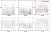 |
Fig. 2 Kinematic dependence on metallicity in Galactic bulge. The red dot and error bar indicate the median values, as well as the 16th and 84th percentiles for each equal-width [Fe/H] bin. Top row: distributions in action-metallicity plane. Note that the median values of Jϕ in each bin could be well fit by a quadratic function. Bottom row: distributions in e/Zmax/η planes. |
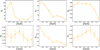 |
Fig. 3 Dependences of action dispersions (defined as standard deviations) and orbital dispersions on metallicity are examined. The action dispersions of metal-poor stars are larger than those of metal-rich stars, suggesting that metal-poor stars may have multiple dynamical origins. The error bar indicates the standard error, which is given by |

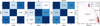 |
Fig. 4 Heat map illustrates similarity of the three clusters based on the distributions of Jr, Jz, and [Fe/H]. The rightmost panel shows the distributions of the three clusters in the Jr/Jtotal–|Jϕ|/Jtotal plane, with the median, 16th percentile, and 84th percentile of [Fe/H] for each cluster indicated in the legend. Cluster 0 has a wide span in the plane and could potentially be clustered into smaller groups when additional quantities are considered. Cluster 1 is the most metal-poor and is supported by both radial and rotational motion. Cluster 2 is the least metal-poor and is mainly supported by rotational motion. |
3.3 The retrograde stars in the Galactic bulge
The retrograde stars (Vϕ < 0) are confined within  kpc of the bulge across all metallicities (see bottom left panel of Figure 5), compared to prograde stars, which are found at
  . This observation is noteworthy, and we briefly discuss the properties of these stars here. In Figure 6, the fraction of retrograde stars in each [Fe/H] bin decreases with increasing metallicity (except for the very metal-rich end). Belokurov & Kravtsov (2022) found that the Galactic disk experienced a process called “spin-up” due to the rapid formation of the MW disk over ∼1–2 Gyr, during which the median Vϕ of the in situ stars increased sharply with increasing metallicity between −1.3 and −0.9. Although our bulge samples are limited to [Fe/H] > −0.8, there is still an evolution in the Vϕ-[Fe/H] plane for [Fe/H] > −0.8 (see Figure 4 in Belokurov & Kravtsov 2022), which possibly explains the decreasing ratio trend if the bulge formed from the disk, such as a clumpy disk origin (Inoue 2012). The high ratio at the very metal-rich end could be attributed to either the fewer data points causing larger scatter, or these very metal-rich stars having a much more complex dynamical origin.
Queiroz et al. (2021) also identified those retrograde stars (which they defined as Vϕ < −50 km/s) using APOGEE DR16 and found that the retrograde stars were more metal-poor and more eccentric than prograde stars (see Figure 5). They speculated that these retrograde stars could be the counterparts of the Splash debris (Belokurov et al. 2020), but contaminated by metal-rich stars, which consists of proto-disk stars heated by the last major merger, featuring [Fe/H] > −0.7 and highly eccentric characteristics. Additionally, the retrograde stars are slightly more [C/N] and α enhanced than the prograde stars, suggesting that they are relatively older (Salaris et al. 2015; Jofré 2021). However, the Splash stars have mean cylindrical radii of 6 ∼ 9 kpc in the solar vicinity, making it difficult to explain why Splash counterparts are observed right in the bulge. Both retrograde metal-poor and metal-rich stars have VR dispersions of ∼116 km/s, which is only about half that of the Splash stars according to the simulation (Liao et al. 2024). Consequently, we excluded the “Splash-counterpart” hypothesis and instead propose that these stars are very likely born in situ in the bulge, given their small galactocentric distances, or that they are from the migration of disk stars with a clumpy origin (Amarante et al. 2020).
3.3.1 The [Mg/Mn]-[Al/Fe] plane
The [Mg/Mn]–[Al/Fe] plane is used to chemically select the accreted populations (Hawkins et al. 2015; Das et al. 2020). The accreted and in situ regions are also referred to as “unevolved” and “evolved” regions, respectively (see Horta et al. (2021) for more details). The MW and its satellites follow different evolutionary paths in this plane, influenced by their initial mass functions and masses. Typically, the evolutionary paths of satellites end at lower [Al/Fe] values, whereas the MW reaches higher [Al/Fe] values (Fernandes et al. 2023). In the [Mg/Mn]–[Al/Fe] plane (see Figure 7), we notice almost no accreted populations in the unevolved region. This is not surprising, as parts of the inner Galactic substructure, such as Heracles, are very metal-poor with a mean [Fe/H] of −1.26. In the vicinity of regions A and B, there is a distinct gap of [Al/Fe] values between the metal-rich stars found in these two regions. The metal-rich stars in region A have [Al/Fe] < −0.15, while the metal-rich stars in region B have [Al/Fe] > −0.10. As can be seen in Figure 7, the low-Al stars are well separated from the rest distributions with a clear gap. According to Fernandes et al. (2023), dwarf galaxies typically end their evolutionary paths in region A, while larger galaxies such as the MW conclude in region B. Therefore, it is possible that the stars in region A are accreted, indicating a recent merger event (i.e., Virgo Radial Merger; Donlon et al. 2019), as these stars are at the end of their evolutionary path. Feuillet et al. (2022) also identified these low-[Al/Fe] (defined as [Al/Fe] < −0.20) metal-rich stars in the Galactic disk using APOGEE DR17 and found they were extremely old, thus suggesting an accretion origin.
To study the correlation of these low-[Al/Fe] metal-rich stars between in the bulge and the disk, we also selected similar stars from the thick and thin disks for comparison, as shown in Figure 8. The disk sample stars are selected with the same quality cuts as the bulge stars but with different spatial constraints: 3.5 < R < 8 kpc and 0 < |z| < 1 kpc. Here, we did not remove the contamination of the metal-poor halo stars either, since we only considered the metal-rich stars. The high-α thick disk and low-α thin disk were separated according to the relation [α/M] = −0.17∗[M/H] + 0.06. We define low-Al metal-rich stars with [Al/Fe] < −0.15 and [Fe/H] > 0. From Figure 8, we observe that the thick disk still exhibits [Al/Fe] evolution with respect to [Fe/H] in the range of 0–0.25, showing a slope of −0.36 from a linear fit of the [Al/Fe]–[Fe/H] plane. By contrast, the thin disk shows a mild evolution with a slope of −0.09, while the bulge exhibits a slope of −0.22, confirming the previous finding that there are chemical similarities between the thick disk and the bulge (Alves-Brito et al. 2010). Moreover, Di Matteo (2016) found that the chemistry of the bulge and Galactic disks became evident when considering the radial and vertical structures, and the thick disk was essential for a whole picture of the bulge (also see Rojas-Arriagada et al. 2017). Among the 179 low-Al metal-rich stars in the bulge, 145 (∼80%) exhibit a thick-disk-like relation, with [α/M] being greater than −0.17∗[M/H] + 0.06. As a result, it is likely that these low-Al metal-rich stars are associated with those found by Feuillet et al. (2022).
Combining the previous analysis on kinematics with this work, it is very possible that the metal-rich stars in the bulge have a disk origin due to migration caused by the growing bar. However, the metal-rich stars are not all contributed by the thin disk as Boin et al. (2024) suggested. The exact origin of the low-Al metal-rich stars is difficult to determine due to the mass-metallicity relation (Brinchmann et al. 2004).
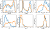 |
Fig. 5 Histograms of retrograde and prograde stars are presented in terms of elemental abundances and orbital parameters. The retrograde stars show a metal-poor peak at ∼ − 0.6 and are more metal-poor than prograde stars. The retrograde stars are also slightly more [C/N]- and α-enhanced than prograde stars, indicating that they are relatively older. The retrograde stars are mainly confined to within rGC ∼ 2 kpc, while the prograde stars have a large rGC of more than 3 kpc. Both retrograde and prograde stars have Zmax < 3 kpc. |
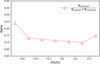 |
Fig. 6 Ratio of retrograde stars to total stars as a function of metallicity. |
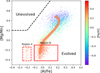 |
Fig. 7 Distributions of bulge stars in the [Mg/Mn]– [Al/Fe] plane show that there are almost no accreted stars in the unevolved region. The wide coral-colored line represents the evolutionary path that fits the observations. The metal-rich stars in region A and region B show a clear gap in [Al/Fe] values, suggesting the low [Al/Fe] metal-rich stars in region A could have an accretion origin. |
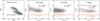 |
Fig. 8 Leftmost panel: disk samples with 3.5 < R < 8 kpc and 0 < |z| < 1 kpc without metal-poor stellar-halo contamination removed. Three right panels: distributions in [Al/Fe]-[Fe/H] plane of thick disk, thin disk, and the bulge. The dashed red line indicates where [Al/Fe]= −0.15. The solid red line represents the linear fit for high-Al ([Al/Fe]) metal-rich stars when 0 < [Fe/H] < 0.25, where m is the slope and b is the intercept. 145 out of 179 low-Al metal-rich bulge stars exhibit thick-disk-like chemical characteristics. |
3.3.2 The elemental-abundance distributions
Figure 9 shows the chemical distributions of α elements (O, Mg, Si, Ca), odd-z elements (Na, Al), the iron-peak element (Mn), and [C/N] ratios. The existing bimodality of [α/Fe]–[Fe/H] and [C/N]–[Fe/H] distributions confirms the former observations (Rojas-Arriagada et al. 2019; Queiroz et al. 2021). The knees of the [α/Fe]–[Fe/H] planes (where α denotes O, Mg, Si, and Ca) are all at [Fe/H] ∼ −0.2, which is higher than previous studies (Hill et al. 2011; Friaça & Barbuy 2017) and also higher than that of thick-disk stars (Bensby et al. 2017; Rojas-Arriagada et al. 2017). This suggests that the star formation rate in the bulge could be higher than previously considered, as there are more Type Ia supernovae dominating over Type II supernovae at later times (Mason et al. 2024), as well as a shorter formation timescale (Lecureur et al. 2007). The production of odd-z elements is metallicity-dependent and depends on the surplus of neutrons from Ne made in the CNO cycle (Kobayashi et al. 2020). As shown in Figure 9, the [Al/Fe]–[Fe/H] distribution also exhibits a bimodality (McWilliam 2016), with low-Al metal-rich stars identified through Gaussian kernel estimation, and a similar knee to those of the α elements. In contrast, the distribution of [Na/Fe]–[Fe/H] does not align with the bulge-evolution model proposed by Kobayashi et al. (2006) with a flat initial mass function (IMF), while the [Mn/Fe]–[Fe/H] distribution is in agreement with the model.
The observed [Na/Fe] shows a flat trend when [Fe/H] < 0 and rises with increasing [Fe/H] in the super-solar range. The Na element is produced in stars of various masses. For massive stars, carbon burning is the main source (Woosley & Weaver 1995), while a neon-sodium (NeNa) cycle is the main source for stars with lower masses. Na could also be produced through Type Ia supernovae. One possible explanation for the observed increase in [Na/Fe] at higher metallicities is that more massive stars are producing Na more efficiently, leading to fewer white dwarfs and thus allowing Na to be enriched more rapidly than Fe over time. The steep rise of [Na/Fe] exhibits a well-behaved, metallicity-dependent sodium yield, although the Na abundance estimates for metal-rich stars may be overestimated due to saturation effects. We also notice that there are stars with lower [C/N] abundance across all metallicities, which suggests that both metal-poor and metal-rich stars contain an adequate number of young stars, implying a complexity of bulge stellar populations.
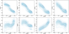 |
Fig. 9 Elemental distributions of bulge in terms of O, Mg, Si, Ca, Na, Al, and Mn elements and [C/N] ratio, with density contours plotted according to the kernel-density estimation (KDE). Notably, the low-Al metal-rich stars are also identified. |
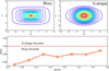 |
Fig. 10 Top row: density functions projected in X–Y plane with Z = 0, where ρ0 is chosen to be 1. Bottom row: relative possibility of supporting a certain profile as a function of metallicity. The dashed red line indicates the same possibility of supporting two profiles. For each [Fe/H] bin, there are 15 bins in the X direction, 15 bins in the Y direction, and three bins in the Z direction. |
3.4 Structural dependence on metallicity in the Galactic bulge
The B/P shape of the bulge has been studied through an RCG star-count method (Stanek et al. 1994; Babusiaux & Gilmore 2005; Ness & Lang 2016). The X shape of the bulge has also been identified through the “split in the red clump” observed in star counts along the line of sight toward the bulge (Ness & Lang 2016). However, there are different viewpoints suggesting that this X shape may be an artifact resulting from the split in RCG stars due to the presence of different stellar populations (López-Corredoira 2016; López-Corredoira et al. 2019). Some simulations (Athanassoula et al. 2017; Semczuk et al. 2022) have revealed that the X shape is most prominent in more metal-rich or younger stars, while a boxy or spheroidal component is clearly observed among more metal-poor or older stars. To avoid confusion, it should be clarified that both the B/P structure and the X shape are manifestations of the same structural feature in the bulge – the X shape is essentially a spatial extension of the boxy/peanut structure, or, more precisely, the X shape is “embedded” within the boxy/peanut configuration (see Figures 3 and 4 of Athanassoula et al. 2017). Moreover, the boxy and spheroid distributions can be related, representing hotter populations according to Debattista et al. (2017).
To quantitatively study the structural dependence on metallicity in the Galactic bulge, we adopted the density functions for both the boxy and X-shaped profiles from López-Corredoira et al. (2005) and Wegg & Gerhard (2013), respectively:
 (3)
(3)
 (4)
(4)
where ![Mathematical equation: ${s_1} = {\mathop{\rm Max}\nolimits} \left[ {2100{\rm{pc}},\sqrt {{x^2} + {{{y \over {0.7}}}^2}} } \right],{s_2} = \sqrt {{{(x - 1.5z)}^2} + {y^2}} ,{s_3} = \sqrt {{{(x + 1.5z)}^2} + {y^2}} $](/articles/aa/full_html/2025/12/aa55965-25/aa55965-25-eq8.png) . The parametrization is provided by López-Corredoira (2017). Following Chrobáková et al. (2022), we minimized the χ2 to fit the two models, which is defined as follows:
. The parametrization is provided by López-Corredoira (2017). Following Chrobáková et al. (2022), we minimized the χ2 to fit the two models, which is defined as follows:
 (5)
(5)
 , where ρ1 corresponds to the Poisson error of each spatial bin and ρ1 is inversely proportional to the bin size. When ρi,data = 0, σi = ρ1. We divided the data into 26 bins in the X direction, 26 bins in the Y direction, and ten bins in the Z direction. We find that the spatial distribution of the data supports a boxy profile more than an X-shaped profile with a smaller χ2 value. Here, we did not calculate the corresponding probabilities from the cumulative distribution function, as the probabilities vary significantly with different bin sizes. After testing with different bin sizes, we find that the bulge data generally support the boxy profile with smaller χ2 values more.
We used the ratio  as the relative probability of supporting a certain profile, as a function of [Fe/H] as well as stellar age. As shown in Figure 10, the observed data across all metallicities support a boxy profile. However, the ratio exhibits an upward trend with increasing metallicity, indicating that metal-rich stars are more likely to support an X-shaped profile than metal-poor stars, which is in agreement with the simulation from Athanassoula et al. (2017). However, in the study by Zoccali et al. (2018), metal-rich stars exhibit a distinct boxy profile when observed from the Sun’s perspective, which contradicts the simulation from Athanassoula et al. (2017). The discrepancy may arise because the simulation introduced a major merger event 8–10 Gyr ago, rather than allowing the bulge to evolve secularly driven by bar instability. From Figure 10, although metal-rich stars show a higher tendency toward X-shaped structures, we can see that they still predominantly exhibit a boxy profile. This suggests that while the major merger may influence the spatial distribution, it is likely not the dominant factor.
It needs to be noted that we do not include comparisons with other survey data or the sample selection effects, as these are beyond the scope of this work. However, we can still clearly observe how the structure of the bulge depends on metallicity and stellar age, which has not been extensively discussed when using observational data.
4 Discussion and summary
Using elemental abundances from APOGEE DR17 and astrometric data from Gaia DR3, we examined how kinematics, elemental abundances, and the spatial distribution of bulge stars correlate with metallicity. We confirm the trend of line-of-sight velocity dispersions along the minor axis of the bulge, noting that metal-rich stars exhibit this trend with a turning point at |b| ∼ 6.5°, while metal-poor stars do not. This indicates that metal-rich stars are trapped by bar instability, whereas metal-poor stars have a more complex dynamical origin. In the MDF of bulge stars, we identified six peaks, with the most metal-rich peak showing the highest prominence. Metal-poor stars exhibit larger dispersions in actions compared to metal-rich stars, indicating that metal-poor stars are kinematically incoherent, while metal-rich stars are relatively coherent. This suggests that metal-poor stars may have multiple dynamical origins.
In addition, we applied GMM in (Jr,Jϕ and [Fe/H]) space for both metal-poor and metal-rich stars. According to the SC estimation criterion, metal-rich stars are better represented by a single cluster, suggesting a shared dynamical origin. In contrast, at least three distinct clusters are identified among the metal-poor stars. We also noticed that the retrograde stars are centered within  of the bulge. Generally, more metal-rich stars exhibit a lower retrograde ratio, which can be interpreted as evidence that the bulge has a disk origin and that these stars experienced a “spin-up” process within the disk. These retrograde stars could also be in situ stars without a “Splash” origin if the bulge has a clumpy disk origin (Amarante et al. 2020).
In the [Mg/Mn]–[Al/Fe] plane of bulge sample stars, we observe that a few metal-rich stars with low Al abundances may be associated with accreted substructures in the disk (Feuillet et al. 2022). If this is the case, ∼80% of these stars exhibit a thick-disk-like α-abundance pattern, and they may have migrated from the thick disk due to the growing bar. However, it is diffi-cult to determine whether these stars are indeed accreted, as they are too metal-rich to have originated from typical dwarf galaxies. The elemental distributions of bulge stars are generally aligned with the theoretical model proposed by Kobayashi et al. (2006). The sodium-enhanced and metal-rich stars are well represented in our samples, indicating that there could be more massive stars in the bulge than we previously considered, requiring a much flatter IMF or probably an IMF in logarithmic normal form (e.g., see the comparison in Figure 21 from Johnson et al. 2014). In the previous study, Lecureur et al. (2007) found that bulge stars have higher O, Mg, and Al abundances than disk stars when [Fe/H] > −0.5, which also suggests a possible top-heavy IMF for the Galactic bulge (see also Cescutti & Matteucci 2011). We also briefly studied the spatial distribution dependence on metallicity and found that, across all metallicities, the stars have a higher probability of supporting a boxy profile of the bulge. Metal-rich stars show higher probabilities of exhibiting an X-shaped profile compared to metal-poor stars; however, they still generally support a boxy profile.
In summary, the origins of metal-poor stars still need further exploration in future surveys. Conversely, the metal-rich stars are similar in kinematics, and there is clear evidence that they have a disk origin. However, the metal-rich stars could not only originate from the thin disk, as simulations suggest, but also from the thick disk.
Acknowledgements
We thank the anonymous referee for insightful suggestions that have greatly improved this manuscript. This work was supported by National Key R&D Program of China No. 2024YFA1611900, and the National Natural Science Foundation of China (NSFC Nos. 11973042, 11973052). Funding for the Sloan Digital Sky Survey IV has been provided by the Alfred P. Sloan Foundation, the U.S. Department of Energy Office of Science, and the Participating Institutions. SDSS-IV acknowledges support and resources from the Center for High Performance Computing at the University of Utah. The SDSS website is www.sdss4.org. SDSS-IV is managed by the Astrophysical Research Consortium for the Participating Institutions of the SDSS Collaboration including the Brazilian Participation Group, the Carnegie Institution for Science, Carnegie Mellon University, Center for Astrophysics | Harvard & Smithsonian, the Chilean Participation Group, the French Participation Group, Instituto de Astrofísica de Canarias, The Johns Hopkins University, Kavli Institute for the Physics and Mathematics of the Universe (IPMU) / University of Tokyo, the Korean Participation Group, Lawrence Berkeley National Laboratory, Leibniz Institut für Astrophysik Potsdam (AIP), Max-Planck-Institut für Astronomie (MPIA Heidelberg), Max-Planck-Institut für Astrophysik (MPA Garching), Max-Planck-Institut für Extraterrestrische Physik (MPE), National Astronomical Observatories of China, New Mexico State University, New York University, University of Notre Dame, Observatário Nacional / MCTI, The Ohio State University,Pennsylvania State University, Shanghai Astronomical Observatory, United Kingdom Participation Group, Universidad Nacional Autónoma de México, University of Arizona, University of Colorado Boulder, University of Oxford, University of Portsmouth, University of Utah, University of Virginia, University of Washington, University of Wisconsin, Vanderbilt University, and Yale University. This work has made use of data from the European Space Agency (ESA) mission Gaia (https://www.cosmos.esa.int/gaia), processed by the Gaia Data Processing and Analysis Consortium (DPAC, https://www.cosmos.esa.int/web/gaia/dpac/consortium). Funding for the DPAC has been provided by national institutions, in particular the institutions participating in the Gaia Multilateral Agreement.
References
- Abbott, C. G., Valluri, M., Shen, J., & Debattista, V. P. 2017, MNRAS, 470, 1526 [NASA ADS] [CrossRef] [Google Scholar]
- Abdurro’uf, Accetta, K., Aerts, C., et al. 2022, ApJS, 259, 35 [NASA ADS] [CrossRef] [Google Scholar]
- Alves-Brito, A., Meléndez, J., Asplund, M., Ramírez, I., & Yong, D. 2010, A&A, 513, A35 [NASA ADS] [CrossRef] [EDP Sciences] [Google Scholar]
- Amarante, J. A. S., Beraldo e Silva, L., Debattista, V. P., & Smith, M. C. 2020, ApJ, 891, L30 [NASA ADS] [CrossRef] [Google Scholar]
- Arentsen, A., Starkenburg, E., Martin, N. F., et al. 2020, MNRAS, 491, L11 [Google Scholar]
- Athanassoula, E. 2005, MNRAS, 358, 1477 [NASA ADS] [CrossRef] [Google Scholar]
- Athanassoula, E., Rodionov, S. A., & Prantzos, N. 2017, MNRAS, 467, L46 [Google Scholar]
- Babusiaux, C. 2016, PASA, 33, e026 [NASA ADS] [CrossRef] [Google Scholar]
- Babusiaux, C., & Gilmore, G. 2005, MNRAS, 358, 1309 [NASA ADS] [CrossRef] [Google Scholar]
- Babusiaux, C., Gómez, A., Hill, V., et al. 2010, A&A, 519, A77 [NASA ADS] [CrossRef] [EDP Sciences] [Google Scholar]
- Babusiaux, C., Katz, D., Hill, V., et al. 2014, A&A, 563, A15 [NASA ADS] [CrossRef] [EDP Sciences] [Google Scholar]
- Barbuy, B., Hill, V., Zoccali, M., et al. 2013, A&A, 559, A5 [NASA ADS] [CrossRef] [EDP Sciences] [Google Scholar]
- Belokurov, V., & Kravtsov, A. 2022, MNRAS, 514, 689 [NASA ADS] [CrossRef] [Google Scholar]
- Belokurov, V., Sanders, J. L., Fattahi, A., et al. 2020, MNRAS, 494, 3880 [Google Scholar]
- Bennett, M., & Bovy, J. 2019, MNRAS, 482, 1417 [NASA ADS] [CrossRef] [Google Scholar]
- Bensby, T., Yee, J. C., Feltzing, S., et al. 2013, A&A, 549, A147 [NASA ADS] [CrossRef] [EDP Sciences] [Google Scholar]
- Bensby, T., Feltzing, S., Gould, A., et al. 2017, A&A, 605, A89 [NASA ADS] [CrossRef] [EDP Sciences] [Google Scholar]
- Boin, T., Di Matteo, P., Khoperskov, S., et al. 2024, A&A, 692, A13 [NASA ADS] [CrossRef] [EDP Sciences] [Google Scholar]
- Bovy, J. 2015, ApJS, 216, 29 [NASA ADS] [CrossRef] [Google Scholar]
- Brinchmann, J., Charlot, S., White, S. D. M., et al. 2004, MNRAS, 351, 1151 [Google Scholar]
- Cescutti, G., & Matteucci, F. 2011, A&A, 525, A126 [NASA ADS] [CrossRef] [EDP Sciences] [Google Scholar]
- Chrobáková, Ž., López-Corredoira, M., & Garzón, F. 2022, A&A, 666, L13 [NASA ADS] [CrossRef] [EDP Sciences] [Google Scholar]
- Combes, F., & Sanders, R. H. 1981, A&A, 96, 164 [NASA ADS] [Google Scholar]
- Das, P., Hawkins, K., & Jofré, P. 2020, MNRAS, 493, 5195 [NASA ADS] [CrossRef] [Google Scholar]
- Deason, A. J., Belokurov, V., Koposov, S. E., & Lancaster, L. 2018, ApJ, 862, L1 [Google Scholar]
- Debattista, V. P., Ness, M., Gonzalez, O. A., et al. 2017, MNRAS, 469, 1587 [Google Scholar]
- Di Matteo, P. 2016, PASA, 33, e027 [CrossRef] [Google Scholar]
- Donlon, T. II, Newberg, H. J., Weiss, J., Amy, P., & Thompson, J. 2019, ApJ, 886, 76 [NASA ADS] [CrossRef] [Google Scholar]
- Erwin, P., & Debattista, V. P. 2016, ApJ, 825, L30 [NASA ADS] [CrossRef] [Google Scholar]
- Fernandes, L., Mason, A. C., Horta, D., et al. 2023, MNRAS, 519, 3611 [NASA ADS] [CrossRef] [Google Scholar]
- Feuillet, D. K., Feltzing, S., Sahlholdt, C., & Bensby, T. 2022, ApJ, 934, 21 [Google Scholar]
- Fisher, D. B., & Drory, N. 2016, in Astrophysics and Space Science Library, 418, Galactic Bulges, eds. E. Laurikainen, R. Peletier, & D. Gadotti, 41 [Google Scholar]
- Forbes, D. A. 2020, MNRAS, 493, 847 [Google Scholar]
- Friaça, A. C. S., & Barbuy, B. 2017, A&A, 598, A121 [NASA ADS] [CrossRef] [EDP Sciences] [Google Scholar]
- Gaia Collaboration (Prusti, T., et al.) 2016, A&A, 595, A1 [NASA ADS] [CrossRef] [EDP Sciences] [Google Scholar]
- Gaia Collaboration (Vallenari, A., et al.) 2023, A&A, 674, A1 [NASA ADS] [CrossRef] [EDP Sciences] [Google Scholar]
- Gardner, E., Debattista, V. P., Robin, A. C., Vásquez, S., & Zoccali, M. 2014, MNRAS, 438, 3275 [Google Scholar]
- Garzon, D. N., Frankel, N., Zari, E., Xiang, M., & Rix, H.-W. 2024, ApJ, 972, 155 [NASA ADS] [CrossRef] [Google Scholar]
- Gonzalez, O. A., Rejkuba, M., Zoccali, M., et al. 2011, A&A, 530, A54 [NASA ADS] [CrossRef] [EDP Sciences] [Google Scholar]
- Gonzalez, O. A., Zoccali, M., Vasquez, S., et al. 2015, A&A, 584, A46 [NASA ADS] [CrossRef] [EDP Sciences] [Google Scholar]
- Han, X., Wang, H.-F., Carraro, G., et al. 2025, ApJ, 985, 32 [Google Scholar]
- Hawkins, K., Jofré, P., Masseron, T., & Gilmore, G. 2015, MNRAS, 453, 758 [NASA ADS] [CrossRef] [Google Scholar]
- Hill, V., Lecureur, A., Gómez, A., et al. 2011, A&A, 534, A80 [NASA ADS] [CrossRef] [EDP Sciences] [Google Scholar]
- Horta, D., & Schiavon, R. P. 2024, arXiv e-prints [arXiv:2410.16374] [Google Scholar]
- Horta, D., Schiavon, R. P., Mackereth, J. T., et al. 2021, MNRAS, 500, 1385 [Google Scholar]
- Inoue, S. 2012, in Astronomical Society of the Pacific Conference Series, 458, Galactic Archaeology: Near-Field Cosmology and the Formation of the Milky Way, eds. W. Aoki, M. Ishigaki, T. Suda, T. Tsujimoto, & N. Arimoto, 227 [Google Scholar]
- Jofré, P. 2021, ApJ, 920, 23 [CrossRef] [Google Scholar]
- Johnson, C. I., Rich, R. M., Kobayashi, C., et al. 2013, ApJ, 765, 157 [Google Scholar]
- Johnson, C. I., Rich, R. M., Kobayashi, C., Kunder, A., & Koch, A. 2014, AJ, 148, 67 [Google Scholar]
- Johnson, C. I., Rich, R. M., Simion, I. T., et al. 2022, MNRAS, 515, 1469 [NASA ADS] [CrossRef] [Google Scholar]
- Khoperskov, S., Di Matteo, P., Steinmetz, M., et al. 2025, A&A, 700, A90 [NASA ADS] [CrossRef] [EDP Sciences] [Google Scholar]
- Kobayashi, C., Umeda, H., Nomoto, K., Tominaga, N., & Ohkubo, T. 2006, ApJ, 653, 1145 [NASA ADS] [CrossRef] [Google Scholar]
- Kobayashi, C., Karakas, A. I., & Lugaro, M. 2020, ApJ, 900, 179 [Google Scholar]
- Kormendy, J., & Kennicutt, R. C. Jr., 2004, ARA&A, 42, 603 [NASA ADS] [CrossRef] [Google Scholar]
- Kruijssen, J. M. D., Pfeffer, J. L., Chevance, M., et al. 2020, MNRAS, 498, 2472 [NASA ADS] [CrossRef] [Google Scholar]
- Lecureur, A., Hill, V., Zoccali, M., et al. 2007, A&A, 465, 799 [NASA ADS] [CrossRef] [EDP Sciences] [Google Scholar]
- Leung, H. W., & Bovy, J. 2019, MNRAS, 489, 2079 [CrossRef] [Google Scholar]
- Li, Z.-Y., & Shen, J. 2015, ApJ, 815, L20 [Google Scholar]
- Lian, J., Zasowski, G., Hasselquist, S., et al. 2021, MNRAS, 500, 282 [Google Scholar]
- Liao, X., Li, Z.-Y., Simion, I., et al. 2024, ApJ, 967, 5 [Google Scholar]
- López-Corredoira, M. 2016, A&A, 593, A66 [NASA ADS] [CrossRef] [EDP Sciences] [Google Scholar]
- López-Corredoira, M. 2017, ApJ, 836, 218 [CrossRef] [Google Scholar]
- López-Corredoira, M., Cabrera-Lavers, A., & Gerhard, O. E. 2005, A&A, 439, 107 [NASA ADS] [CrossRef] [EDP Sciences] [Google Scholar]
- López-Corredoira, M., Lee, Y. W., Garzón, F., & Lim, D. 2019, A&A, 627, A3 [NASA ADS] [CrossRef] [EDP Sciences] [Google Scholar]
- Lucey, M., Hawkins, K., Ness, M., et al. 2019, MNRAS, 488, 2283 [NASA ADS] [CrossRef] [Google Scholar]
- Lucey, M., Hawkins, K., Ness, M., et al. 2022, MNRAS, 509, 122 [Google Scholar]
- Lütticke, R., Dettmar, R. J., & Pohlen, M. 2000, A&AS, 145, 405 [NASA ADS] [CrossRef] [EDP Sciences] [Google Scholar]
- Mason, A. C., Crain, R. A., Schiavon, R. P., et al. 2024, MNRAS, 533, 184 [NASA ADS] [CrossRef] [Google Scholar]
- Matteucci, F., Grisoni, V., Spitoni, E., et al. 2019, MNRAS, 487, 5363 [Google Scholar]
- McMillan, P. J. 2017, MNRAS, 465, 76 [NASA ADS] [CrossRef] [Google Scholar]
- McTier, M. A. S., Kipping, D. M., & Johnston, K. 2020, MNRAS, 495, 2105 [NASA ADS] [CrossRef] [Google Scholar]
- McWilliam, A. 2016, PASA, 33, e040 [NASA ADS] [CrossRef] [Google Scholar]
- McWilliam, A., Rich, R. M., & Smecker-Hane, T. A. 2003, ApJ, 592, L21 [NASA ADS] [CrossRef] [Google Scholar]
- McWilliam, A., & Zoccali, M. 2010, ApJ, 724, 1491 [NASA ADS] [CrossRef] [Google Scholar]
- Meléndez, J., Asplund, M., Alves-Brito, A., et al. 2008, A&A, 484, L21 [NASA ADS] [CrossRef] [EDP Sciences] [Google Scholar]
- Minniti, D. 1996, ApJ, 459, 579 [Google Scholar]
- Molero, M., Matteucci, F., Spitoni, E., Rojas-Arriagada, A., & Rich, R. M. 2024, A&A, 687, A268 [NASA ADS] [CrossRef] [EDP Sciences] [Google Scholar]
- Nataf, D. M., Udalski, A., Gould, A., Fouqué, P., & Stanek, K. Z. 2010, ApJ, 721, L28 [NASA ADS] [CrossRef] [Google Scholar]
- Ness, M., & Freeman, K. 2016, PASA, 33, e022 [Google Scholar]
- Ness, M., Freeman, K., Athanassoula, E., et al. 2013a, MNRAS, 430, 836 [CrossRef] [Google Scholar]
- Ness, M., Freeman, K., Athanassoula, E., et al. 2013b, MNRAS, 432, 2092 [CrossRef] [Google Scholar]
- Ness, M., & Lang, D. 2016, AJ, 152, 14 [NASA ADS] [CrossRef] [Google Scholar]
- Ness, M., Zasowski, G., Johnson, J. A., et al. 2016, ApJ, 819, 2 [NASA ADS] [CrossRef] [Google Scholar]
- Okamoto, T. 2013, MNRAS, 428, 718 [NASA ADS] [CrossRef] [Google Scholar]
- Queiroz, A. B. A., Chiappini, C., Perez-Villegas, A., et al. 2021, A&A, 656, A156 [NASA ADS] [CrossRef] [EDP Sciences] [Google Scholar]
- Rich, R. M. 1990, ApJ, 362, 604 [NASA ADS] [CrossRef] [Google Scholar]
- Rich, R. M., Origlia, L., & Valenti, E. 2012, ApJ, 746, 59 [NASA ADS] [CrossRef] [Google Scholar]
- Rix, H.-W., Chandra, V., Andrae, R., et al. 2022, ApJ, 941, 45 [NASA ADS] [CrossRef] [Google Scholar]
- Rix, H.-W., Chandra, V., Zasowski, G., et al. 2024, ApJ, 975, 293 [NASA ADS] [CrossRef] [Google Scholar]
- Rojas-Arriagada, A., Recio-Blanco, A., Hill, V., et al. 2014, A&A, 569, A103 [NASA ADS] [CrossRef] [EDP Sciences] [Google Scholar]
- Rojas-Arriagada, A., Recio-Blanco, A., de Laverny, P., et al. 2017, A&A, 601, A140 [NASA ADS] [CrossRef] [EDP Sciences] [Google Scholar]
- Rojas-Arriagada, A., Zoccali, M., Schultheis, M., et al. 2019, A&A, 626, A16 [NASA ADS] [CrossRef] [EDP Sciences] [Google Scholar]
- Rojas-Arriagada, A., Zasowski, G., Schultheis, M., et al. 2020, MNRAS, 499, 1037 [Google Scholar]
- Salaris, M., Pietrinferni, A., Piersimoni, A. M., & Cassisi, S. 2015, A&A, 583, A87 [NASA ADS] [CrossRef] [EDP Sciences] [Google Scholar]
- Schönrich, R., & Binney, J. 2009, MNRAS, 396, 203 [Google Scholar]
- Schönrich, R., Binney, J., & Dehnen, W. 2010, MNRAS, 403, 1829 [NASA ADS] [CrossRef] [Google Scholar]
- Schultheis, M., Rojas-Arriagada, A., García Pérez, A. E., et al. 2017, A&A, 600, A14 [NASA ADS] [CrossRef] [EDP Sciences] [Google Scholar]
- Semczuk, M., Dehnen, W., Schönrich, R., & Athanassoula, E. 2022, MNRAS, 517, 6060 [Google Scholar]
- Stanek, K. Z., Mateo, M., Udalski, A., et al. 1994, ApJ, 429, L73 [NASA ADS] [CrossRef] [Google Scholar]
- Uttenthaler, S., Schultheis, M., Nataf, D. M., et al. 2012, A&A, 546, A57 [NASA ADS] [CrossRef] [EDP Sciences] [Google Scholar]
- Wegg, C., & Gerhard, O. 2013, MNRAS, 435, 1874 [Google Scholar]
- Woosley, S. E., & Weaver, T. A. 1995, ApJS, 101, 181 [Google Scholar]
- Wylie, S. M., Gerhard, O. E., Ness, M. K., et al. 2021, A&A, 653, A143 [NASA ADS] [CrossRef] [EDP Sciences] [Google Scholar]
- Wyse, R. F. G., Gilmore, G., & Franx, M. 1997, ARA&A, 35, 637 [NASA ADS] [CrossRef] [Google Scholar]
- Yan, T.-S., Shi, J.-R., Tian, H., Zhang, W., & Zhang, B. 2022, Res. Astron. Astrophys., 22, 025007 [Google Scholar]
- Zoccali, M., Hill, V., Lecureur, A., et al. 2008, A&A, 486, 177 [NASA ADS] [CrossRef] [EDP Sciences] [Google Scholar]
- Zoccali, M., Valenti, E., & Gonzalez, O. A. 2018, A&A, 618, A147 [NASA ADS] [CrossRef] [EDP Sciences] [Google Scholar]
All Tables
Comparisons between peaks of MDF from this study and those from previous literature, where the parentheses indicate the
All Figures
|
Fig. 1 Left panel: line-of-sight velocity dispersions (in units of km/s) across 0 < |b| < 10° along the minor axis (|l| < 2°) of the bulge. The solid red and blue lines represent metal-rich and metal-poor stars, respectively. The dashed lines represent the metal-rich and metal-poor subsamples, while the black cross indicates EMR stars. Right panel: MDF of bulge. Six peaks have been identified with a prominence of 0.25, as indicated by the black arrows. |
| In the text | |
|
Fig. 2 Kinematic dependence on metallicity in Galactic bulge. The red dot and error bar indicate the median values, as well as the 16th and 84th percentiles for each equal-width [Fe/H] bin. Top row: distributions in action-metallicity plane. Note that the median values of Jϕ in each bin could be well fit by a quadratic function. Bottom row: distributions in e/Zmax/η planes. |
| In the text | |
|
Fig. 3 Dependences of action dispersions (defined as standard deviations) and orbital dispersions on metallicity are examined. The action dispersions of metal-poor stars are larger than those of metal-rich stars, suggesting that metal-poor stars may have multiple dynamical origins. The error bar indicates the standard error, which is given by |
| In the text | |
|
Fig. 4 Heat map illustrates similarity of the three clusters based on the distributions of Jr, Jz, and [Fe/H]. The rightmost panel shows the distributions of the three clusters in the Jr/Jtotal–|Jϕ|/Jtotal plane, with the median, 16th percentile, and 84th percentile of [Fe/H] for each cluster indicated in the legend. Cluster 0 has a wide span in the plane and could potentially be clustered into smaller groups when additional quantities are considered. Cluster 1 is the most metal-poor and is supported by both radial and rotational motion. Cluster 2 is the least metal-poor and is mainly supported by rotational motion. |
| In the text | |
|
Fig. 5 Histograms of retrograde and prograde stars are presented in terms of elemental abundances and orbital parameters. The retrograde stars show a metal-poor peak at ∼ − 0.6 and are more metal-poor than prograde stars. The retrograde stars are also slightly more [C/N]- and α-enhanced than prograde stars, indicating that they are relatively older. The retrograde stars are mainly confined to within rGC ∼ 2 kpc, while the prograde stars have a large rGC of more than 3 kpc. Both retrograde and prograde stars have Zmax < 3 kpc. |
| In the text | |
|
Fig. 6 Ratio of retrograde stars to total stars as a function of metallicity. |
| In the text | |
|
Fig. 7 Distributions of bulge stars in the [Mg/Mn]– [Al/Fe] plane show that there are almost no accreted stars in the unevolved region. The wide coral-colored line represents the evolutionary path that fits the observations. The metal-rich stars in region A and region B show a clear gap in [Al/Fe] values, suggesting the low [Al/Fe] metal-rich stars in region A could have an accretion origin. |
| In the text | |
|
Fig. 8 Leftmost panel: disk samples with 3.5 < R < 8 kpc and 0 < |z| < 1 kpc without metal-poor stellar-halo contamination removed. Three right panels: distributions in [Al/Fe]-[Fe/H] plane of thick disk, thin disk, and the bulge. The dashed red line indicates where [Al/Fe]= −0.15. The solid red line represents the linear fit for high-Al ([Al/Fe]) metal-rich stars when 0 < [Fe/H] < 0.25, where m is the slope and b is the intercept. 145 out of 179 low-Al metal-rich bulge stars exhibit thick-disk-like chemical characteristics. |
| In the text | |
|
Fig. 9 Elemental distributions of bulge in terms of O, Mg, Si, Ca, Na, Al, and Mn elements and [C/N] ratio, with density contours plotted according to the kernel-density estimation (KDE). Notably, the low-Al metal-rich stars are also identified. |
| In the text | |
|
Fig. 10 Top row: density functions projected in X–Y plane with Z = 0, where ρ0 is chosen to be 1. Bottom row: relative possibility of supporting a certain profile as a function of metallicity. The dashed red line indicates the same possibility of supporting two profiles. For each [Fe/H] bin, there are 15 bins in the X direction, 15 bins in the Y direction, and three bins in the Z direction. |
| In the text | |
Current usage metrics show cumulative count of Article Views (full-text article views including HTML views, PDF and ePub downloads, according to the available data) and Abstracts Views on Vision4Press platform.
Data correspond to usage on the plateform after 2015. The current usage metrics is available 48-96 hours after online publication and is updated daily on week days.
Initial download of the metrics may take a while.