| Issue |
A&A
Volume 704, December 2025
|
|
|---|---|---|
| Article Number | A129 | |
| Number of page(s) | 15 | |
| Section | Astrophysical processes | |
| DOI | https://doi.org/10.1051/0004-6361/202556012 | |
| Published online | 03 December 2025 | |
Relativistic reflection within an extended hot plasma geometry
1
Dr. Karl Remeis-Sternwarte & ECAP, Friedrich-Alexander-Universität Erlangen-Nürnberg, Sternwartstr. 7, 96049 Bamberg, Germany
2
NASA Goddard Space Flight Center, X-ray Astrophysics Laboratory, 8800 Greenbelt Road, Greenbelt, MD 20771, USA
3
Cahill Center for Astrophysics, California Institute of Technology, 1216 East California Boulevard, Pasadena, CA 91125, USA
4
Centre for Astrophysics Research, University of Hertfordshire, College Lane, Hatfield AL10 9AB, United Kingdom
5
Institut für Theoretische Physik und Astrophysik, Universität Würzburg, Emil-Fischer-Str. 31, 97074 Würzburg, Germany
6
Institut für Theoretische Physik, Goethe Universität, Max-von-Laue-Str. 1, 60438 Frankfurt, Germany
7
Max-Planck-Institut für Radioastronomie, Auf dem Hügel 69, 53121 Bonn, Germany
8
H. H. Wills Physics Laboratory, Tyndall Avenue, Bristol BS8 1TL, United Kingdom
9
Center for Astrophysics | Harvard & Smithsonian, 60 Garden Street, Cambridge, MA 02138, USA
⋆ Corresponding author: This email address is being protected from spambots. You need JavaScript enabled to view it.
Received:
18
June
2025
Accepted:
27
September
2025
Abstract
Context. The reflection of X-rays at the inner accretion disk around black holes imprints relativistically broadened features in the observed spectrum. Aside from the black hole properties and the ionization and density of the accretion disk, these features also depend on the location and geometry of the primary source of X-rays, often referred to as the corona.
Aims. We present a fast general relativistic model for spectral fitting of a radially extended, ring-like corona above the accretion disk.
Methods. A common approach used to explain observed X-ray reflection spectra is the lamp post geometry, which assumes a point-like source on the rotational axis of the black hole. While it is typically able to explain the observations, this geometric model does not allow for any constraint to be placed on the radial size of the corona. We therefore extended the publicly available relativistic reflection model RELXILL by implementing a radially extended, ring-like primary source.
Results. With the new RELXILL model allowing us to vary the position of the primary source in two dimensions, we present simulated line profiles and spectra and discuss the implications of carrying out a data fitting, in comparison to the lamp post model. We applied this extended RELXILL model to XMM-Newton and NuSTAR data of the radio-quiet Seyfert-2 active galactic nucleus (AGN) ESO 033-G002. The new model describes the data well and we are able to constrain the distance of the source to the black hole to be less than three gravitational radii, while the angular position of the source is poorly constrained.
Conclusions. We show that a compact, radially extended corona close to the innermost stable circular orbit is able to explain the observed relativistic reflection as well as the lamp post corona does. This model has been made freely available to the community.
Key words: accretion / accretion disks / black hole physics / X-rays: general
© The Authors 2025
 Open Access article, published by EDP Sciences, under the terms of the Creative Commons Attribution License (https://creativecommons.org/licenses/by/4.0), which permits unrestricted use, distribution, and reproduction in any medium, provided the original work is properly cited.
This article is published in open access under the Subscribe to Open model. This email address is being protected from spambots. You need JavaScript enabled to view it. to support open access publication.
1. Introduction
X-rays carry direct information from the innermost region around black holes (BHs). Thermal radiation from an accretion disk (Shakura & Sunyaev 1973) is upscattered by inverse Compton effect in a hot plasma, often called the “corona”, which is located close to the BH (Sunyaev & Titarchuk 1980; Haardt & Maraschi 1993). Some of these hard X-rays then irradiate the disk, where they are reprocessed in a process called reflection (George & Fabian 1991; Matt et al. 1993; Krolik et al. 1994; Blackman 1999; Ross & Fabian 2005; García & Kallman 2010). The strongest feature of the reflection spectrum is typically the fluorescent Fe Kα line at 6.4 keV, while the detailed shape of spectrum depends on the parameters of the accretion disk such as its ionization and density (García et al. 2016).
If reflection takes place in the vicinity of the BH, strong general relativistic energy shifts and special relativistic Doppler boosting affect the spectral shape (Lightman & White 1988; Fabian et al. 1989; Tanaka et al. 1995; Reynolds & Nowak 2003; Dauser et al. 2010). These effects depend on the observer’s viewing angle and carry information about the matter and space-time in the vicinity of the BH (see, e.g., Bambi et al. 2021). This includes the BH’s spin (Reynolds 2021), properties of the disk such as its density and ionization, and, in particular, the location and geometry of the primary source of hard X-rays.
Earlier studies (e.g., Wilms et al. 2001; Miller et al. 2002; Fabian et al. 2004; Dauser et al. 2012; Keck et al. 2015) have shown that steep disk irradiation profiles, also called emissivity profiles, are required to explain the observations. The simplest geometry that explains this strong focusing of the irradiation onto the inner accretion disk is the “lamp post” geometry (e.g., Martocchia & Matt 1996; Martocchia et al. 2002; Vaughan & Fabian 2004; Dauser et al. 2013), where the primary source geometry is approximated as an emitting point source on the BH’s spin axis. The success of this geometry in describing spectra of many sources has been interpreted in a way that the primary source cannot be significantly extended in size (e.g., Fabian et al. 2014; Parker et al. 2015; Duro et al. 2016; Beuchert et al. 2017; Walton et al. 2020, 2021), consistent with X-ray timing studies (Kara et al. 2016; Cackett et al. 2021) and data from gravitationally lensed quasars (Vernardos et al. 2024, and therein).
Several models for relativistic reflection exist to study the physical properties of BHs and their innermost regions (see, e.g., Bambi 2024). Currently, RELXILL (Dauser et al. 2014; García et al. 2014) is the most widely used and significantly advanced relativistic reflection model. It predicts the reflected and direct parts of the spectra (Dauser et al. 2016), including a self-consistent treatment of the ionization gradient based on the irradiation profile and an α-disk model density profile of Shakura & Sunyaev (1973) and takes into account returning radiation, the secondary reflection produced by reflected photons returning to the disk (Dauser et al. 2022). Other advanced models, such as RELTRANS (Ingram et al. 2019; Mastroserio et al. 2021), KYN (Dovčiak et al. 2004), or REFLKERR (Niedźwiecki & Życki 2008; Niedźwiecki et al. 2019) address other aspects such as time-resolved studies, reflection from the plunging region, or polarization. Many of these models also assume a lamp post geometry.
Theoretical and observational work shed light on possible configurations of the innermost region. The primary source can be stationary or outflowing (Beloborodov 1999; Dauser et al. 2013) or be variable (e.g., Wilkins & Gallo 2015; Chainakun & Young 2017; Kara et al. 2019). Several distinct regions are sometimes required to describe the data (e.g., Fürst et al. 2015; Petrucci et al. 2018). Recently, X-ray polarimetry data from several sources have been interpreted as evidence for a radially extended primary source (e.g., Krawczynski et al. 2022), albeit without fully accounting for effects such as the contribution of returning radiation to the polarization (see Ratheesh et al. 2024).
Significant efforts have been made in recent years to describe more realistic primary source geometries. These include vertically extended, line-like primary sources in RELXILL (Dauser et al. 2013) and RELTRANS (Lucchini et al. 2023), radially extended ring-like sources (e.g., Miniutti et al. 2003; Miniutti & Fabian 2004; Suebsuwong et al. 2006; Niedźwiecki & Życki 2008), slab and spherical geometries (e.g., Niedźwiecki 2005; Wilkins & Fabian 2012; Wilkins & Gallo 2015), and cylindrical and conical geometries (e.g., Gonzalez et al. 2017; Szanecki et al. 2020; Uttley & Malzac 2025). A disk-like geometry was considered by Riaz et al. (2022). More recently, conical and wedge-like geometries have also been implemented in the ray-tracing code KERRC (Krawczynski & Beheshtipour 2022), while spherical geometry has been included in the ray-tracing code MONK (Zhang et al. 2019, 2024) and a relativistic reflection model for off-axis point sources was released by Feng et al. (2025).
In this paper, we extend the RELXILL framework by allowing the primary source to be radially extended. RELXILL is the perfect choice for this generalization, as it is a very fast model allowing for the spectral fitting of complex data sets and includes a detailed description of the accretion disk ionization and density gradient. We chose a ring-like primary source geometry as the simplest extension of the lamp post geometry, since multiple ring sources of different sizes and heights can be readily combined to model extended primary sources of arbitrary axially symmetric geometry. A ring-like model is also a good description of any compact off-axis source, because any off-axis point source will appear as an axially symmetric ring when observed over typical observation timescales of current X-ray observatories. In Sect. 2, we describe the new ring source model. We then summarize in Sect. 3 the influence of the radial size of the primary source on the reflected spectra. In Sect. 4, we describe how we applied the ring model to the radio-quiet Seyfert 2 galaxy ESO 033-G002. Finally, we discuss the new model and the results in Sect. 5.
2. Modeling reflection from axisymmetric sources
We considered a geometrically thin accretion disk irradiated by a primary source, which is described by a geometrically thin ring at height, h, above the equatorial plane. The ring has radius, x, and is centered on the BH’s rotational axis (see Fig. 1), such that x = 0 recovers the lamp post geometry. We defined the dimensionless spin of the BH as a = J/M, ranging from −0.998 to 0.998 (Thorne 1974). Distances are given in units of gravitational radii, rg = GM/c2, unless otherwise stated. We set the speed of light, the gravitational constant, and the BH mass equal to unity, c = G = M = 1.
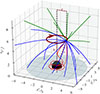 |
Fig. 1. Individually selected isotropically distributed photon trajectories emitted by a point source at h = 5rg, x = 2rg. The BH has a spin of a = 0.998 and is located at x′ = 0, y′ = 0, z′ = 0. The event horizon is illustrated in black. The accretion disk plane is z′ = 0. The dark red ring is the primary source after axial averaging. Red trajectories plunge into the BH, green trajectories escape the system, and blue trajectories hit the accretion disk, where they will be reflected. The point source is rotating in the direction denoted by the dark red arrow with a velocity vφ as given by Eq. (7). We also display the corresponding spherical coordinates of the source, (r, θ), related to (h, x) by Eq. (4). |
2.1. Basic equations
For our ray tracing procedure, we used the Kerr (1963) metric in Boyer & Lindquist (1967) coordinates (Bardeen et al. 1972),
 (1)
(1)
where
 (2)
(2)
with
 (3)
(3)
and where the source height, h, and radius, x, are given by
 (4)
(4)
The inner edge of the geometrically thin accretion disk in the equatorial plane around the BH is given by the innermost stable circular orbit (ISCO), rISCO. The Keplerian velocity of the accretion disk is (Bardeen et al. 1972):
 (5)
(5)
where rd is the spherical radius, r, measured in the metric equatorial plane, namely, the disk radius.
The Lorentz-factor, in general and for circular equatorial orbits (Bardeen et al. 1972), is
 (6)
(6)
We use the common assumption (e.g., Miniutti & Fabian 2004; Niedźwiecki 2005; Niedźwiecki & Życki 2008; Wilkins & Fabian 2012) that the primary source is corotating with the accretion disk. This assumption is more plausible than a stationary source if we are positing that the primary source consists of material ejected from the disk and some kind of (partial) angular momentum conservation holds. For rings outside the ISCO, x ≥ rISCO, the angular velocity of the source is the Keplerian velocity of the accretion disk at distance, rd = x. Following Niedźwiecki & Życki (2008), inside the ISCO, x < rISCO, the angular velocity of the ring, Ω, is assumed to be constant and given by the disk velocity at rISCO. The only nonzero component of the three-velocity is, therefore,
 (7)
(7)
For x = 0, vφ = 0, meaning a stationary point source. However, we stress that the actual velocity in the plunging region inside the ISCO is more complicated, as radial and vertical components of the velocity become non-negligible (see, e.g., Pu et al. 2016; Mummery & Balbus 2023). Thus, the photons that are beamed in the direction of motion will redistribute the resulting disk irradiation (see, e.g., Niedźwiecki & Życki 2008; Dauser et al. 2013). We also note that the RELXILL model allows for a vertical velocity of the primary source and, therefore, it includes the beaming of the flux in the direction of the rotation axis. Contrary to the case of a corotating source, a static source (vφ = 0, but note frame dragging, ω) will boost less photons to the outer disk and there will be less of a Doppler shift, such that the blueshift in the line decreases (see, e.g., Niedźwiecki & Życki 2008, for a comparison of static and corotating ring sources).
With these assumptions, following Niedźwiecki (2005) the energy shift of the photons from a source with initial rest frame energy, Esource, to the energy, Edisk, at the point of impact with the disk is
![Mathematical equation: $$ \begin{aligned} g = \frac{{E_\mathrm{disk} }}{{E_\mathrm{source} }} = \frac{\left[\gamma e^{-\nu } \left(1 - {\Omega _\mathrm{K} } (r_\mathrm{d} ) \lambda \right)\right]_\mathrm{disk} }{\left[\gamma e^{-\nu } \left(1 - {\Omega } (x) \lambda \right)\right]_\mathrm{source} }, \end{aligned} $$](/articles/aa/full_html/2025/12/aa56012-25/aa56012-25-eq8.gif) (8)
(8)
where γ, e−ν, Ω, and ΩK are taken at the locations of the source (“source”) and the disk (“disk”), respectively, λ = L/E is the dimensionless angular momentum of the photon1 (see Appendix A for the derivation of this equation). Equation (8) reduces to the lamp post case for λ = 0 (see, e.g., Dauser et al. 2013). For a given (r, θ, φ), λ depends on the initial direction of motion of the photon and can take positive and negative values.
2.2. Ray-tracing for an off-axis source
To perform ray-tracing, we use the YNOGK code for null-geodesics in the Kerr metric (Yang & Wang 2013), computing the velocity profile of the emitting source with Eq. (7). For each parameter combination, we use a Monte Carlo approach. We assume a point source that emits isotropically in its rest frame, drawing the emission angles of individual photons from uniform distributions for φ ∈ [0, 2π), and cos θ ∈ [ − 1, 1].
Figure 1 shows selected simulated photon trajectories for a rapidly rotating BH with a spin of a = 0.998. In the frame of rest of an observer at infinity, the photons are boosted in the direction of the rotation due to the fast azimuthal velocity of the source. Depending on their initial direction, photons emitted from the ring will either fall into the BH, hit the accretion disk, or escape to infinity. We assume that photons crossing the equatorial plane between the ISCO and the event horizon are scattered or advected inward by the in-flowing matter (Agol & Krolik 2000) and are therefore captured by the BH.
2.3. Disk irradiation by a ring source
A ring source can be modeled as a combination of multiple off-axis point sources at different azimuthal angles. Due to the azimuthal symmetry, each of these sources will produce the same irradiating flux on the disk, such that the irradiation profile (i.e., the radial-dependent incident flux on the accretion disk) can be derived by simulating a single off-axis point source and then integrating the resulting flux distribution on the accretion disk over the azimuthal coordinate (see also Wilkins & Fabian 2012).
We performed a set of simulations for different values of spin, a, height, h, and source radius, x, at a fixed azimuthal angle ϕ = 0. From these simulations, we derived the specific photon flux, Φ(rd, ϕ, Esource), incident on a disk element at radius, rd, and azimuth, ϕ, of width, drd and dϕ, and an energy, Esource, in the source rest frame. The flux is proportional to the number of photons incident on a given disk area divided by this area. Following Dauser et al. (2013), for each disk annulus, we determined the irradiating flux at energy Edisk = gEsource (Eq. (8)) in the frame of rest of the disk by integrating over the azimuth and radius,
 (9)
(9)
where AKerr is the area of the annulus at radius, rd, and width, Δrd, as seen by a distant observer (Wilkins & Fabian 2012):
 (10)
(10)
and γ is the Lorentz factor of the disk element (Eq. (6)), accounting for the disk’s rotation. The proper area of the disk annulus in the frame of the disk is therefore given by γAKerr.
As the irradiating flux depends on the primary source spectral shape, integration over the azimuthal coordinate in Eq. (9) can be performed only for a known spectral shape. Assuming that the primary source emits a power-law spectrum in its rest frame2 (see Dauser et al. 2013), Φ(Esource)∝Esource−Γ, with photon index Γ, and using discrete annuli with sufficiently small Δrd,
 (11)
(11)
2.3.1. Energy shift from the off-axis sources
The main difference between a ring and a lamp post geometry is that there is a large range of different photon trajectories incident on the same disk radius. This is because photons emitted from different locations on the ring can hit the same disk element. Since the Doppler boosting can be strongly different for these photons, this affects the irradiation profile seen by the accretion disk.
In Fig. 2, we show how the energy shift of isotropically emitted photons from off-axis sources located on two compact rings at h = 3rg depends on radius. For a very compact ring, x = 2rg, all photons emitted by different points on the ring experience a similar energy shift at small disk radii, increasing to factors of ∼20 at large radii. An increase in ring radius (x = 5rg) leads to a larger spread of energy shifts at small radii, and a lower spread at large radii, respectively. As the ring is corotating with the disk, for rd ∼ x the range of energy shifts drops to zero. For radii larger (smaller) than the corotation radius, the disk rotation is slower (faster) than that of the emitting source. We note that for a given rd the time-dilation term of the metric (Eq. (1)), e−ν, also influences the energy shift, causing it to decrease.
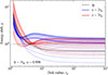 |
Fig. 2. Energy shift, g, of photons propagating from off-axis sources, located at h = 3rg, at two ring radii x = 2rg (blue lines) and x = 5rg (red lines), and BH spin of a = 0.998. Photon trajectories are selected from an isotropic distribution of the initial photon directions in the rest frame of the sources. Lighter lines show energy shifts of photons emitted by the off-axis sources located on the same ring at different azimuthal angles. Thick lines represent the resulting averaged energy shifts over the disk annuli. The dashed black line corresponds to the energy shift of the photons from a lamp post source with h = 3rg. |
For a qualitative comparison with the lamp post, we also computed the average energy shift of all photons incident on the given disk annulus (Fig. 2, thick lines). Averaging this value over azimuth yields the energy shift of the ring. The energy shift is a blue-shift, g > 1, for all radii, leading to a Doppler boost of the irradiating flux. In contrast, irradiating photons from a lamp post are redshifted at large radii, resulting in a reduced flux (Fig. 2, dashed line). For sources that are similar to a lamp post (x ≲ rISCO) and close enough to the BH (h less than a few rg), the emitted photons will also be red-shifted if incident at large radii.
2.3.2. Disk irradiation profiles
Using Eq. (9), we calculated the irradiating flux on the accretion disk, which is often called the “emissivity profile”, for a ring-like primary source. Figure 3 shows a selection of characteristic irradiating profiles for rings at different heights and radii. In general, the profiles follow the typical steepening toward the ISCO and converge toward the flat-space irradiating flux of F ∝ rd−3 for large radii. The ring geometry also leads to a flattening of the profile at radii directly underneath the ring.
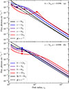 |
Fig. 3. Disk irradiation flux profiles for varying emitting ring radii, x, for (a) a ring at h = 3rg and (b) a ring of varying height with radius fixed at x = 3rg, a BH spin of a = 0.998, and an irradiating source with Γ = 2. The solid black line is for the lamp post case, x = 0, for h = 3rg in (a) and h = 6rg in (b). The dashed line shows a power-law flux ∝rd−3. Markers of the same color on each curve show the disk radius equal to the primary source radius, rd ≡ x. The normalization of the fluxes is set to the non-relativistic limit at large radii (see Appendix B). |
For a fixed source height, with increasing source radius the flux is redistributed towards larger disk radii (Fig. 3a). For x ≳ h, a secondary peak forms below the ring. This behavior is expected for simple geometric reasons. For a source relatively close to the disk, h ≲ x, most photons will hit the disk below the ring, forming a local flux maximum at rd ∼ x, if the source is more extended radially than vertically. In addition, light-bending modifies the irradiating profiles (Sect. 2.2), as radiation is focused onto the inner part of the disk. Similar to the lamp post geometry, this effect is strongest for rd < 10rg, and further increases irradiation at the disk radius directly underneath the ring, rd ≈ x. For the smallest ring radii, the local flux maximum emerges at slightly larger radii than the ring radius because light bending “pulls” the flux emitted directly below the ring away to even smaller radii.
For a fixed ring radius, x, with increasing height more flux impacts the outer disk and less flux is focused towards the inner edge (Fig. 3b). Even for the highest ring source considered here, h = 12rg, the irradiation profile is still steep at the innermost radii. As long as x ≲ h, the irradiation profile stays similar to that of a lamp post at a similar or larger height. The local maximum at rd ∼ x is replaced by a flattening for rings with h > x. Crucially for the physical interpretation of observed data, we find that the irradiation profiles due to ring sources with relatively small radii can mimic the irradiation profiles of lamp posts with larger heights. For example, profiles with h = 3rg, x = 3rg and h = 6rg, x = 0rg differ significantly only over a very small range of radii.
3. Ring source model for relativistic reflection
With the irradiation profiles for the extended ring-like primary source, we calculated the relativistic line broadening and the resulting reflection spectra for such a geometry. We implemented them as part of the RELXILL model framework (Dauser et al. 2014; García et al. 2014), such that the model can directly fit the observed spectra of accreting BH systems and constrain the parameters of the primary source. We refer to Appendix C for a verification of our code.
3.1. Implementation of the ring geometry in RELXILL
The RELXILL framework is well suited to implement a ring-like primary source, as it is designed in a modular way and we only need to implement a new irradiation profile (Eq. (9)). The major complexity is to account for the large spread of energy shifts (Sect. 2.3.1) and to apply the correct normalization between direct and reflected flux, including a relativistic lensing of the ring source (see also Ingram et al. 2019; Feng et al. 2025). After that we re-use the full RELXILL setup for the computation of the non-relativistic reflection in the rest-frame of the accretion disk (García & Kallman 2010; García et al. 2013) and its propagation to the observer (Dauser et al. 2010).
In RELXILL, the disk irradiation profile is constructed from pre-calculated tables that contain the relevant parameters of the ray-tracing simulations. For a given set of input parameters, the table values are linearly interpolated. To implement the ring source in RELXILL, we therefore pre-calculate a table extending the spin-height grid to include the new radius parameter, x. To obtain a well-sampled photon flux, Φ, we simulate 108 isotropically distributed photons for each grid point. Additionally, the energy shift values, g, are stored, such that the irradiation profile can be calculated for any value of the photon index Γ from Eq. (11) or any more general spectral shape, Eq. (9). As there is a range of energy shifts of photons incident on one annulus at radius, rd (Sect. 2.3.1), we bin the photon trajectories in energy shift in 20 bins and store the relative flux value of each bin in the table (see Appendix B). In order to calculate the primary spectrum normalization and reflection fraction, we also store the photon fractions reaching the disk, qdisk, infinity, qesc, and BH, qbh. As the direct spectrum is also affected by the energy shift and gravitational lensing, we also store these data (see Appendix A for the detailed calculation).
By adding the radial size of the ring source, x, we were able to define a new flavor of the RELXILL model, named RELXILL_RING. We built it on the basis of the most advanced RELXILL model, RELXILLLP_CP, which assumes a Comptonization primary spectrum modeled by NTHCOMP (Zdziarski et al. 1996). We also include effects of the self-consistent ionization gradient in the disk and a self-consistent treatment of the returning reflected radiation, based on Dauser et al. (2022). The model is publicly available as part of the RELXILL model package3.
3.2. Line reflection spectra
We investigated the effect of the location and radius of the ring-like primary source on a single relativistic line profile. As general line profiles of radially extended sources have been presented in a variety of publications (e.g., Miniutti et al. 2003; Miniutti & Fabian 2004; Niedźwiecki & Życki 2008; Dauser et al. 2010, 2013; Riaz et al. 2022), here we focus on comparing the ring sources with their most relevant counterparts, point-like lamp post sources. For the comparison, we used spherical coordinates (r, θ) to define the source position (Eq. (4)), since r has the most significant effect on the line shape and the angular position of the source has only a secondary effect due to Doppler shifts (as we explain later in this section). For clarity, conversions between the quantities (r, θ) and (h, x) are given in Table 1. A lamp post source at height h = r corresponds to θ = 0°.
Figure 4 shows line profiles for sources at different spherical radii and polar angles. For any source with a distance to the BH of r = 3rg (Fig. 4a), the line is very broad, with a strong red wing. For increasing polar angle of the source (i.e., increasing ring size), the velocity of the ring increases from zero to its maximum value at the ISCO, such that more photons are boosted away from the inner disk and experience a larger blueshift. This increase in velocity compared to the stationary lamp post causes the blue wing of the line to slightly brighten and the overall line shape to narrow.
 |
Fig. 4. Line profiles for a ring geometry simulated with RELXILL. We display the geometric parameters of the ring in terms of spherical radii, r, and polar angles, θ. The parameters are uniquely related to height and ring radius through Eq. (4). For ease of comparison, we also convert these values to heights and radii in Table 1. (a) Varying polar angle of the primary source, θ, for two spherical radii, r = 3rg (dashed lines) and r = 9rg (solid lines), with a = 0.998. (b) Varying the spherical radius of the primary source, r, with two polar angles of the primary source, θ = 30° (solid lines) and θ = 0° (dashed lines, the lamp post case), with a = 0.998. (c) Varying the BH spin, a, for a source spherical radius fixed at ISCO value, r = rISCO, and θ = 60°. ISCO radii are 1.24rg, 6rg, 9rg for a = 0.998, 0.0, −0.998, respectively. To convert the quantities (r, θ) to (h, x), we provide the Table 1. All lines are normalized to have the same integrated photon flux. The photon index is Γ = 2 and the inclination to the observer is i = 30°. |
Values of (r, θ) and corresponding (h, x) for several spins.
Increasing the source distance to the BH (i.e., expanding the spherical radius) leads to the line narrowing. This effect prevails regardless of the polar angle (i.e., the ring radius). The main reason for this behavior is that less flux is focused towards the BH and, therefore, fewer reflected photons come from the innermost accretion disk. For r ≳ 5rg, a double-horned skew-symmetric line feature arises from the strong Doppler shift of the photons due to both the disk and the source rotation.
Figure 4c shows how the line shape changes with spin, a, for a source located at a distance to the BH equal to the inner edge of the accretion disk, that is, r = rISCO. As the inner edge of the accretion disk moves outwards for a smaller BH spin, this distance r also increases. We show sources with two polar angles, a lamp post with θ = 0°, and a source with θ = 60°, corresponding to a source almost above the ISCO, at a height of 0.5rISCO (see Table 1). As commonly known (see, e.g., Dauser et al. 2013), for any disk irradiation a broad line is produced only in the case of high spin, which is also the case for our ring-like source (however, see Reynolds & Begelman 1997, for a discussion of emission from the plunging region). Differences between the line profiles for a lamp post and the ring source are more distinct in the high spin case. For non-rotating and counter-rotating BHs, the line shapes are more similar, irrespective of the angle.
In summary, a ring primary source instead of a lamp post source does not lead to substantially different line profiles. The most important result is that the line profiles depend mainly on the distance to the BH (i.e., the spherical radius). Increasing the polar angle, θ, leads to a slightly narrower line that is similar to slightly increasing the height of the lamp post. This can for example be seen in Fig. 4b, where the line shape of the lamp post for (r = 10rg, θ = 0° ) is in between the ring source for (r = 5rg, θ = 30° ) and (r = 10rg, θ = 30° ).
3.3. Relativistic reflection spectra
To illustrate the effects of changing normalization and energy shifts on the spectra, we show (in Fig. 5) both the direct and reflected components of the relativistic reflection spectra for ring-like primary sources. We assumed a maximally spinning BH, a = 0.998, and a source at a small height above the disk plane, h = 3rg, in this case and disregard the returning radiation to focus on the main effect of changing the radius of the ring-like source. We keep all other RELXILL parameters at their default values.
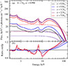 |
Fig. 5. Relativistic reflection spectra for varying ring radius, x. (a) Solid lines show simulated reflected spectra for BH spin of a = 0.998, height of the primary source, h = 3rg, and varying ring radius. Dashed lines show the primary spectra. Different colored lines correspond to different ring radii. The black line corresponds to the lamp post case, x = 0. The spectra are normalized setting BOOST = 1 in RELXILL, such that the reflection fraction is predicted from the geometry of the isotropically emitting primary source. Returning radiation is turned off. All other parameters of RELXILL are set to their default values, i.e., the iron abundance is AFe = 1, the inclination is i = 30°, the disk inner edge is at rISCO, the disk outer edge is at 400rg, the photon index is Γ = 2, the disk ionization is log ξ = 3.1, the disk density log n = 1015 cm−3, and the electron temperature kTe = 60 keV. (b) Ratio between the given reflected spectrum of the ring and the lamp post spectrum, re-normalized to the same flux. |
We find that the total observed flux increases monotonically with increasing ring radius. The primary component drops for x ∼ rISCO ≈ 1.2rg, while the reflected component increases rapidly with x. This behavior is due to a combination of geometric and relativistic effects. The reflected flux increases strongly with the energy boost from the source to the disk, with fewer photons advected into the BH. The fraction of photons hitting the disk reaches its maximum at ∼1.8rg ≈ 1.5rISCO, while the escaping fraction has a minimum at the same radius and, hence, the reflection fraction also reaches its maximum. For small ring sizes, the primary flux drops due to general-relativistic lensing near the BH, which redistributes more flux towards high inclinations with respect to the observer, that is, even if the flux escapes, it still bends toward the equatorial plane and disk. For inclinations of i ≳ 60°, the lensing focuses the flux toward the observer, thus increasing the primary component.
For sources with x ∼ 1–2rISCO (1.2–2.5rg), the equivalent width of the broad iron line reaches its maximum, which is about three times higher than that found for lamp posts. As noted above, the primary continuum reaches its minimum level for the same ring radii. For larger source radii, the equivalent width stays above the lamp post level, although lower than the ISCO case. This increase in the equivalent width (i.e., stronger lines) found for ring sources can potentially influence the measurement of iron abundances in spectral fits; in other words, fitting a lamp post would yield a higher iron abundance to explain a broad line than models with an extended source. Overall, a source above the ISCO produces the strongest relativistic reflection relative to the primary flux and, therefore, also the strongest broad lines.
4. Application to ESO 033-G002
To illustrate the application of the new reflection model, we went on to apply it to an observation of the Seyfert-2 active galactic nucleus (AGN) ESO 033-G002 that is well known to show strong relativistic reflection. The data have been analyzed in detail by Walton et al. (2021, hereafter W21). These authors showed that this source has a strong relativistic reflection component in the spectrum, which can be described well by a lamp post primary source very close to the BH (h ≲ 2rg). The strong reflection in this source makes it a well-suited target for a first application of our new model.
4.1. Observation and data reduction
We use data from a joint observation of ESO 033-G002 in 2021 June with XMM-Newton (Jansen et al. 2001, ObsID 0863050201, 109 ks for EPIC-pn and 125 ks for both EPIC-MOS detectors) and NuSTAR (Harrison et al. 2013, ObsID 0863050201, 172 ks), which were published by W21.
For XMM-Newton’s instruments EPIC-pn, EPIC-MOS1, and EPIC-MOS2, we reduced and extracted the data over the 0.3–10 keV energy band with XMM-Newton SAS version 21.0.0. For the extraction, we used a circular region with a 35″ radius; for the background, we used a circular region with 70″ radius on the same chip. We set applyabsfluxcorr=yes to obtain a better agreement between the effective areas of the EPIC-detectors and NuSTAR, which led to larger cross-calibration constants between XMM-Newton and NuSTAR compared to W214. After extraction, data from EPIC-MOS1 and EPIC-MOS2 are combined into one dataset. We use optimal binning (Kaastra & Bleeker 2016) to rebin the spectra, ensuring a minimum signal-to-noise ratio of 5.
We reduce and extract 4–78 keV spectra for NuSTAR-FPMA and -FPMB with the NuSTAR Data Analysis Software version 2.1.4 and NuSTAR calibration database v20241015. We extracted the source products and response from a circular region with 90″ radius and estimated the background from a 100″ radius region on the same chip. The spectra were again binned with the optimum binning algorithm, ensuring a signal-to-noise ratio of 5. We note that the NuSTAR spectrum becomes background-dominated at ≳40 keV, resulting in only a few wide bins.
4.2. General model set-up
To fit the data, we used ISIS (Houck & Denicola 2000), applying a similar model as W21. We used the most recent RELXILL model (v2.7) for the lamp post (RELXILLLP_CP) and the ring source geometry (RELXILL_RING) described in Sect. 3.1. Following W21, we assumed that the relativistic reflector is ionized, modeled by XSTAR with the same model grid as W21 and neutral absorption via the full and partially covering absorbers, TBABSfull and TBABSpart, respectively (Wilms et al. 2000). We used the TBNEW_FEO model, which has the iron abundance of the absorber as a free parameter, tied to the RELXILL iron abundance. We model the distant reflection with XILLVER_CP and the scattered nuclear flux with NTHCOMPscat. The CP flavor of the RELXILL model also includes a separate NTHCOMP component that represents the primary continuum. Different to W21 we describe the emission spectrum from collisionally ionized diffuse gas with APEC5 (Smith et al. 2001; Foster et al. 2012) instead of MEKAL (Mewe et al. 1986; Liedahl et al. 1995). All of the model components are cosmologically redshifted by the host galaxy redshift z = 0.0181 (Tueller et al. 2010) and affected by Galactic absorption, which we modeled with TBABSGal for a fixed absorption column of NH = 8.95 × 1020 cm−2 (HI4PI Collaboration 2016). We used the wilm-abundances (Wilms et al. 2000), instead of grsa (Grevesse & Sauval 1998) used by W21. Since we applied a flux correction to the data, as recommended by the new extraction guides (Sect. 4.1), we took into account the cross-calibration between NuSTAR and EPIC-pn by applying a multiplicative constant DETCONST to the NuSTAR spectra.
The full expression of the base model is: DETCONST × tbabsGal × (APEC + NTHCOMPscat + XILLVER_CP + (TBABSfull × TBABSpart × XSTAR × RELXILL)). RELXILL stands for the relativistic reflection model, which is either the lamp post model RELXILLLP_CP in the base model or the new extended model from this work.
4.3. Lamp post models
We reproduce W21’s results by applying the lamp post model to the data (Model 1a). Identical to W21-Model 2a, we use RELXILLLP_CP6 to model relativistic reflection, allowing for a free, but constant disk ionization and density, with no returning radiation. Due to our choice of the optional extraction argument applyabsfluxcorr=yes, we found flux cross-calibration constants at ∼1.25 and ∼1.29 for the NuSTAR focal plane modules, FPMA and FPMB, with respect to EPIC-pn (Sect. 4.1). Table 2 gives all the best-fit parameters.
Comparison of the lamp post and extended models for ESO 033-G002.
We found a good fit with χred2 = 458.0/401 = 1.142 and we were able to reproduce the parameters in W21. The only exception was that we obtained a higher hydrogen column density of the fully and partially covering absorbers, which was expected because we used the abundances wilm instead of grsa.
Next, we relaxed the assumption on the lamp post by adding returning radiation and self-consistent ionization for an α-disk density profile. The latter is especially important for a rapidly spinning BH and a compact primary source (Dauser et al. 2022), which is the case for ESO 033-G002. This model, Model 1b, yields again a good description of the data (χred2 = 458.8/401 = 1.144, see Table 2). Including returning radiation, we find a larger upper limit on the height of the primary source, which increases from 2.0rg to 3.2rg. The reason is that in the fit the increase in the source height, which decreases the energy shift, is compensated for by the contribution of returning radiation. The ionization gradient, as opposed to constant ionization, results in lower ionization of the disk overall. Instead of an average ionization of  , a maximum ionization7 is now
  . The limit on disk density, log n, increases inversely proportionally from log n < 17.7 to log n < 18.3.
Overall, the updated model Model 1b does not differ significantly from Model 1a. The ionization, log ξ, is the only parameter that is outside the confidence limit of the previous Model 1a. Therefore, Model 1b will serve as a reference for comparison with the extended RELXILL model from this work.
4.4. Ring model
After finding the lamp post best fit (Model 1b), we switched to RELXILL_RING and allowed the radial position of the primary source, x, to vary freely (Model 2a). The best fit model and residuals are shown in Fig. 6 and Fig. 7 (see Table 2 for all fit parameters). Relativistic reflection is the main contribution to the model at energies ≳1 keV, except for the iron line at 6.4 keV, which originates in the distant reflector. The primary flux component of RELXILL is about an order of magnitude lower than the reflected component, due to the compact primary source geometry and rapidly rotating BH, a > 0.93.
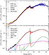 |
Fig. 6. (a) Time-averaged XMM-Newton and NuSTAR spectrum of ESO 033-G002 extracted and binned according to Sect. 4.1 and the full Model 2a in black. (b) Components of the best-fit of Model 2a for ESO 033-G002. The parameters of the fit are listed in Table 2 and the residuals are shown in Fig. 7c. |
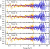 |
Fig. 7. Residuals of the models presented in Table 2. The colors of the data bins have the same meanings as in Fig. 6. |
We found that the new ring-like model describes the data equally well (χ2/D.o.F = 458.6/400) and we found no major differences to the lamp post model in the residuals. The radius of the ring-like primary source is constrained below x < 2.1rg, excluding a primary source with a larger radius. This result is expected since small values of x create line profiles similar to the lamp post (see Fig. 4). The height is constrained to < 2.4rg. All other parameters are comparable to Model 1b within uncertainties.
Additionally, we test Model 2b with the normalization of the reflected and primary spectrum fixed to the one expected from a ring with an isotropic emission pattern (i.e., we fix the parameter BOOST = 1). The results are also shown in Table 2. We do not find significant differences between the two models. The reason being that the spectrum is very reflection dominated, which can also be seen in the fact that Model 2a only sets a lower limit on the boost parameter of BOOST > 0.76. We note that while BOOST values ≫1 are formally allowed by the fit, they can be ruled out as non-physical because such values would require the primary emission to be exceedingly boosted towards the disk. In Fig. 7 we show the residuals of both models, Model 2a and Model 2b, compared to the fits of the lamp post model. There are no significant differences in the residuals between the models.
We show the confidence contours for the radius of the primary source in Fig. 8, comparing Model 2a and Model 2b. Despite the stronger assumption of BOOST = 1 in Model 2b, both models show a similar behavior of a slowly increasing Δχ2 with the ring radius. Only for large source radii, a free normalization between the reflection and the direct spectrum leads to a weaker constraint on the radius. These results confirm that there is no second solution with a large source radius that would describe the data equally well or better than a compact lamp post-like source.
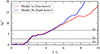 |
Fig. 8. 1D confidence contours for the radius of the primary source, x, calculated for Model 1a and for Model 2b. The horizontal dashed lines show the 1σ, 2σ, and 3σ confidence levels for x values. |
5. Discussion and conclusions
We have developed a new reflection model that describes X-ray reflection for a ring-like source on the symmetry axis of a rotating BH. The emission line profiles and properties of the reflection spectrum indicate (not unsurprisingly) that in the limit of small ring radii, only minor differences are found between the ring-like source and a point source. At large source radii, significant differences in the irradiation profile and in the line profile are present (Sect. 3). This means that it is, in principle, possible to constrain the size of the irradiating medium through X-ray spectral modeling.
In this work, we applied our model to a well-studied observation of ESO 033-G002 (Sect. 4). In the previous study W21 showed that the reflection spectrum can be described by a lamp post. Here, after applying the extended version of RELXILL, an upper limit was found for the radius of the ring-like source of primary X-rays. Specifically, we found h < 2.4rg and x < 2.1rg, We can also exclude the existence of a more extended ring-like source. To our knowledge, this is the first (or at least among the first) direct constraints set on the size of the source of hard X-rays that is solely based on X-ray spectroscopy (noting that other size constraints can be obtained, e.g., from X-ray timing analysis, see Cackett et al. 2021). The availability of the new version of RELXILL means that a significant limitation of earlier reflection models, namely, the assumption of small coronal sizes, has been lifted. This implicit assumption of very small primary source sizes has been one of the major criticisms of lamp post modeling in the literature.
In this section, we address several important aspects and caveats that need to be kept in mind when applying the ring model. We start in Sect. 5.1 with an in-depth discussion of the consequences of our initial result of a small corona for accretion physics, followed by discussions of potential parameter correlations (Sect. 5.2) and our assumption that the primary source has rotational symmetry (Sect. 5.3). We summarize our results in Sect. 5.4.
5.1. Lamp posts and ring-like geometries
The lamp post geometry is a very rudimentary description of a compact spherical primary source on the rotational axis of the BH, described as a point source with a spherically isotropic emission, which is only defined by its height above the BH. Despite these limitations, relativistic reflection models using the lamp post geometry have been very successful in describing observational data of Galactic BH binaries and AGNs. It has been generally assumed that this means that the astrophysical corona is also small. However, before the availability of the model discussed here, there were no tools available that would allow for reflection spectroscopy to be used as a test of the presence of an extended primary source geometry. While a detailed assessment of the validity of the lamp post model is beyond the scope of this study, we summarize the overall behavior below. We note that this discussion should only put earlier fits with the lamp post geometry in perspective. For more reliable estimates of the source geometry, earlier data sets will have to be re-analyzed with a reflection model including a radially extended source.
From the line profiles (see Fig. 4 and Sect. 3.2), we can see that the distance to the BH, r, is mainly influencing the relativistic line broadening; therefore, the shape of the relativistic reflection spectrum for a compact primary source. The position in terms of polar angle only has a minor effect on the line shape. A change of this angle does not produce significantly different line shapes, but can likely be compensated by slightly different values of r. This means that reflection from a point-like source located on the rotational axis produces a similar relativistic line broadening to a radially extended source at a lower height above the disk, but at a similar distance to the BH. Even taking into account the full reflection spectrum including the primary emission, Fig. 5 shows that for a standard lamp post height of h = 3rg, there are only weak differences between the lamp post and a ring source with x < 0.5rISCO modulo normalization.
These general conclusions have been confirmed by our analysis of the data of ESO 033-G002 (Sect. 4), where we find that a ring-like geometry with radius x < 2.1rg gives consistent results to the lamp post geometry. We therefore expect that observations that have been described with lamp post models of a small height are also compatible with ring sources, provided that the ring is only extended by a few gravitational radii. Other extragalactic sources falling in this range include Mrk 335 (Parker et al. 2014), 1H0707−495 (Kara et al. 2015), NGC 4151 (Beuchert et al. 2017), and IRAS 09149−6206 (Walton et al. 2020).
A minimum estimate for the size of the primary source is also necessary for the primary source to be energetically stable and to ensure that enough seed photons from the accretion disk intercept the primary source to allow for a Compton upscattering of the observed spectrum (Dovčiak & Done 2016). By applying this constraint to ESO 033-G002, W21 found that the radius of the spherical source must be at least ∼0.2rg. Although our own model assumes a ring instead of a sphere, with our upper limit of the radius of x < 2.1rg, our results also agree well with this limit as long as the ring is slightly extended.
5.2. Parameter correlations
The analysis of real source data requires us to understand potential correlations between parameters of the model, since they could influence the interpretation of the results. We did so by again using the example of the XMM-Newton and NuSTAR observation of ESO 033-G002 discussed in Sect. 4. Specifically, we study the parameter space through probability distributions of the parameters obtained from Markov chain Monte Carlo (MCMC) sampling (Foreman-Mackey et al. 2013). We used ten walkers for 40 000 steps and remove 5000 first steps as a “burn-in” phase. In total, we used 350 000 parameter combinations. Figure 9 shows the result of MCMC runs8 for Model 2a. Generally, the MCMC results agree well with the best fit values presented in Table 2.
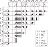 |
Fig. 9. MCMC simulation results for the relevant parameters of Model 2a. Each 1D histogram shows probability distribution of a single parameter values. Each 2D histogram shows probability distribution of each pair of parameters. The red crosses mark the most probable parameter positions according to 1D probability distributions. Additionally, the inset in the lower right corner shows the most probable values with 90% confidence intervals. |
The MCMC runs reveal a strong anti-correlation of the inferred iron abundance, AFe, and the photon index, Γ, and degree of ionization, log ξ. These correlations are not unexpected, and similar to the well-known correlation between Γ and the foreground absorption column, NH. Specifically, since the reflection spectrum increases towards higher energies, a softer spectral shape (i.e., with increasing Γ) can be compensated for by the contribution of the reflection continuum at lower energies. This can be done by increasing AFe, since this changes the contribution of the reflection spectrum at lower energies, especially in combination with the change in log ξ. In addition, a higher disk density (and therefore a lower ionization) also increases the reflected flux at low energies, such that the overall spectral shape appears softer. A similar anti-correlation was found by Tomsick et al. (2018).
The MCMC runs allowed us to understand the correlation between the source’s geometrical parameters. In Fig. 10, we show a more detailed version of the MCMC probability distribution, including lines showing polar coordinates of constant distance to the BH, r, and angular position, θ, of the source. The confidence contours roughly align with the distance of the ring to the BH, r, which has to be < 2.7rg at high significance regardless of the height or radius of the ring, (h, x). In contrast, the position of the source from 0° to 75° is relatively unconstrained. While we can constrain the distance and, therefore, the compactness of the primary source in ESO 033-G002 very well, its actual location is still not well constrained. The source can be both a “lamp post-like” source with a very small radial extent, as well as a “ring-like” source with larger radius at a lower height. This result emphasizes the importance of the distance to the BH in general, regardless of the polar angle.
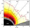 |
Fig. 10. Ring size and height probability distribution with 1σ, 2σ, and 3σ confidence levels, based on the MCMC results (Fig. 9, for Model 2a) extended to lower heights. The color scale shows the probability distribution. The dashed lines show combinations of h and x corresponding to constant polar angles, θ. The black region is limited by the BH event horizon, the gray region denotes RELXILL parameter grid limits. |
Finally, we note that the probability distribution of the BOOST parameter is almost flat and we were only able to obtain a lower limit of BOOST ≳ 0.6. This result indicates that the primary component is not required in the fit and, therefore, the data can be solely described by reflection. This is expected because in the extreme configuration of a very compact primary source, most of the radiation is focused toward the disk and reflected (Dauser et al. 2014). With returning radiation included in the model, this effect becomes even more drastic. Similarly, we did not find any significant correlations between the ring radius, x, and other parameters. Importantly, x is also not correlated with the BH spin, a, such that any combination of small values of h and x is compatible with the observed data.
5.3. Model limitations
Throughout this work, we assumed an axisymmetric primary source. However, intrinsically, the source may be asymmetric or even be an off-axis source rotating around the BH. The resulting spectral variations will be averaged over the exposure time if we apply the reflection model to observations that are longer than the Kepler timescale at the ISCO, TKepler. To first order, for a maximally rotating BH, we have
 (12)
(12)
so that for most realistic, ks-long, exposures the averaging condition is fulfilled.
We also emphasize that the ring geometry used here is still an approximation of a more complicated spatial distribution of matter that we would expect in more realistic models for the inner accretion flow close to the BH. It is important to stress that (similarly to the results of lamp post models), the specific values for the ring radius or height should not be overinterpreted and should only be taken as approximations of the spatial dimensions of even more realistic shapes of the accretion flow.
5.4. Conclusions
We present a new relativistic reflection model with a ring-like primary source of X-rays. The model has been integrated into the publicly available RELXILL reflection model. We find that the main factor influencing the shape of the reflection spectra is the distance of the primary source to the BH, while the polar angle of the source has a weaker effect (Sect. 3.2). This conclusion applies especially for compact sources with ring radii of a few rg where the spectral shape stays similar to the lamp post one, but the reflection fraction is increased (Sect. 3.3). This means that if the true corona is extended, while lamp post models will still describe the data, they will end up overestimating the reflection fraction (Sect. 5.1).
By constraining the radius of the primary source for ESO 033-G002 for the first time, we find a compact geometry of the primary source with a vertical location below ∼3rg and radial location below ∼2rg at a 90% confidence level (Sect. 4.4). We also show that any source at a distance of < 2.7rg to the BH provides an equally good description of the data, with only a weak dependence on the polar angle in a wide range [0° ,75° ].
The more physical representation given by the ring geometry provides us with the opportunity to constrain the size of the primary source. Although the ring source geometry is still overly simplified, it can serve as a basis for further development of more general axisymmetric extended primary source models. For example, slab-like, conical, or spherical primary sources can be easily constructed by combining several emitting rings of different radii and heights. To make further progress, knowledge about the actual geometry of matter is crucial for our understanding of the processes taking place in that compact space-time region. One possible interpretation is that the primary source is connected to the jet launching region, which would provide a connection between the jet base and the accretion flow (e.g., Markoff et al. 2005). We still caution that the real structure of the jet base is expected to be much more complicated than that of a single ring source (e.g., see Dihingia & Fendt 2024, for a review of GRMHD simulations with thin disks). However, the ring model already allows us to fit the radius of the primary source in real time.
Since relativistic reflection spectra mainly depend on the distance to the BH (Sect. 5.1), any spectral fits based on a lamp post geometry are likely compatible also with a source that is radially extended by a few rg. Recent results using X-ray polarimetric data taken by the Imaging X-ray Polarimetry Explorer (IXPE, Weisskopf et al. 2022) of a few selected bright Seyfert galaxies, such as NGC 4151 (Gianolli et al. 2023) and IC 4329A (Ingram et al. 2023), have shown that the medium responsible for creating the polarization has to be roughly perpendicular to the radio jet. These results have been interpreted as evidence of a likely radially extended primary source, as opposed to the compact spherical lamp post that has been employed over the last decade to explain most relativistic reflection spectra. However, these apparent differences between the inferred primary geometries from reflection and polarization studies can be reconciled in light of the results presented here. Furthermore, this would also support the X-ray timing results, which generally prefer small time travel distances between the source and the disk (e.g., Kara et al. 2016; Cackett et al. 2021). The best constraints on the primary source geometry will therefore require a model that includes X-ray polarimetry and reflection for a radially extended primary source.
L is the angular momentum component of the photon parallel to the BH rotational axis and E is the total energy (see Bardeen et al. 1972; Niedźwiecki 2005, for the details of definition and angular dependence).
In all RELXILL models with a primary NTHCOMP spectrum, we use the approximation that the spectrum follows a power law in the relevant energy range, therefore the same transformation applies.
See https://www.cosmos.esa.int/web/xmm-newton/ccf-release-notes and file XMM-CCF-REL-388 about the empirical correction of the EPIC effective area.
Note: starting from RELXILL v2.0, RELXILLLP_CP combines the RELXILL_ION_CP and RELXILL_D_CP flavors that were used in W21; therefore, the name is different in the aforementioned publication, while the underlying model is the same.
The maximum ionization of the α-disk is at rd = (11/9)2rin.
For all MCMC runs, we set the environment variable RELXILL_RENORMALIZE = 1, available since RELXILL v2.4, which redefines the normalization of the total flux to have the same value at 3 keV at each model evaluation. This approach removes the degeneracy of normalization with other parameters (such as the height) and helps the MCMC to converge faster.
Acknowledgments
The authors thank the anonymous referee for the detailed and constructive report with highly useful suggestions on improving the manuscript content. This research is supported by the DFG research unit FOR 5195 ‘Relativistic Jets in Active Galaxies’ (project number 443220636, grant number WI 1860/20-1). DJW acknowledges support from the Science and Technology Facilities Council (STFC; grant code ST/Y001060/1). The results in this paper are in part based on observations obtained with XMM-Newton, an ESA science mission with instruments and contributions directly funded by ESA Member States and NASA. This research has made use of data from the NuSTAR mission, a project led by the California Institute of Technology, managed by the Jet Propulsion Laboratory, and funded by the National Aeronautics and Space Administration. Data analysis was performed using the NuSTAR Data Analysis Software (NuSTARDAS), jointly developed by the ASI Science Data Center (SSDC, Italy) and the California Institute of Technology (USA). This research has made use of ISIS functions (ISISscripts) provided by ECAP/Remeis observatory and MIT (www.sternwarte.uni-erlangen.de/isis/).
References
- Abdikamalov, A. B., Ayzenberg, D., Bambi, C., et al. 2019, ApJ, 878, 91 [Google Scholar]
- Agol, E., & Krolik, J. H. 2000, ApJ, 528, 161 [NASA ADS] [CrossRef] [Google Scholar]
- Baker, F. J. E., & Young, A. J. 2025, MNRAS, staf1770 [Google Scholar]
- Bambi, C. 2024, Frontier Research in Astrophysics– IV (Palermo, Italy) [Google Scholar]
- Bambi, C., Brenneman, L. W., Dauser, T., et al. 2021, Space Sci. Rev., 217, 65 [CrossRef] [Google Scholar]
- Bardeen, J. M., Press, W. H., & Teukolsky, S. A. 1972, ApJ, 178, 347 [Google Scholar]
- Beloborodov, A. M. 1999, ApJ, 510, L123 [CrossRef] [Google Scholar]
- Beuchert, T., Markowitz, A. G., Dauser, T., et al. 2017, A&A, 603, A50 [NASA ADS] [CrossRef] [EDP Sciences] [Google Scholar]
- Blackman, E. G. 1999, MNRAS, 306, L25 [Google Scholar]
- Boyer, R. H., & Lindquist, R. W. 1967, J. Math. Phys., 8, 265 [Google Scholar]
- Cackett, E. M., Bentz, M. C., & Kara, E. 2021, iScience, 24, 102557 [NASA ADS] [CrossRef] [Google Scholar]
- Chainakun, P., & Young, A. J. 2017, MNRAS, 465, 3965 [NASA ADS] [CrossRef] [Google Scholar]
- Dauser, T., Wilms, J., Reynolds, C. S., & Brenneman, L. W. 2010, MNRAS, 409, 1534 [Google Scholar]
- Dauser, T., Svoboda, J., Schartel, N., et al. 2012, MNRAS, 422, 1914 [Google Scholar]
- Dauser, T., García, J., Wilms, J., et al. 2013, MNRAS, 430, 1694 [NASA ADS] [CrossRef] [Google Scholar]
- Dauser, T., García, J., Parker, M. L., Fabian, A. C., & Wilms, J. 2014, MNRAS, 444, L100 [NASA ADS] [CrossRef] [Google Scholar]
- Dauser, T., García, J., Walton, D. J., et al. 2016, A&A, 590, A76 [NASA ADS] [CrossRef] [EDP Sciences] [Google Scholar]
- Dauser, T., García, J., Joyce, A., et al. 2022, MNRAS, 514, 3965 [NASA ADS] [CrossRef] [Google Scholar]
- Dihingia, I. K., & Fendt, C. 2024, in New Frontiers in GRMHD Simulations, eds. C. Bambi, Y. Mizuno, S. Shashank, & F. Yuan (Singapore: Springer), 327 [Google Scholar]
- Dovčiak, M., & Done, C. 2016, AN, 337, 441 [Google Scholar]
- Dovčiak, M., Karas, V., & Yaqoob, T. 2004, ApJS, 153, 205 [Google Scholar]
- Duro, R., Dauser, T., Grinberg, V., et al. 2016, A&A, 589, A14 [NASA ADS] [CrossRef] [EDP Sciences] [Google Scholar]
- Fabian, A. C., Rees, M. J., Stella, L., & White, N. E. 1989, MNRAS, 238, 729 [Google Scholar]
- Fabian, A. C., Miniutti, G., Gallo, L., et al. 2004, MNRAS, 353, 1071 [Google Scholar]
- Fabian, A. C., Parker, M. L., Wilkins, D. R., et al. 2014, MNRAS, 439, 2307 [NASA ADS] [CrossRef] [Google Scholar]
- Feng, Y., Yuan, Y.-F., & Zhang, S.-N. 2025, ApJ, 984, 173 [Google Scholar]
- Foreman-Mackey, D., Hogg, D. W., Lang, D., & Goodman, J. 2013, PASP, 125, 306 [Google Scholar]
- Foster, A. R., Ji, L., Smith, R. K., & Brickhouse, N. S. 2012, ApJ, 756, 128 [Google Scholar]
- Fürst, F., Nowak, M. A., Tomsick, J. A., et al. 2015, ApJ, submitted [arXiv:1506.01381] [Google Scholar]
- García, J., & Kallman, T. R. 2010, ApJ, 718, 695 [CrossRef] [Google Scholar]
- García, J., Dauser, T., Reynolds, C. S., et al. 2013, ApJ, 768, 146 [Google Scholar]
- García, J., Dauser, T., Lohfink, A., et al. 2014, ApJ, 782, 76 [Google Scholar]
- García, J. A., Fabian, A. C., Kallman, T. R., et al. 2016, MNRAS, 462, 751 [Google Scholar]
- George, I. M., & Fabian, A. C. 1991, MNRAS, 249, 352 [Google Scholar]
- Gianolli, V. E., Kim, D. E., Bianchi, S., et al. 2023, MNRAS, 523, 4468 [NASA ADS] [CrossRef] [Google Scholar]
- Gonzalez, A. G., Wilkins, D. R., & Gallo, L. C. 2017, MNRAS, 472, 1932 [Google Scholar]
- Grevesse, N., & Sauval, A. J. 1998, Space Sci. Rev., 85, 161 [Google Scholar]
- Haardt, F., & Maraschi, L. 1993, ApJ, 413, 507 [Google Scholar]
- Harrison, F. A., Craig, W. W., Christensen, F. E., et al. 2013, ApJ, 770, 103 [Google Scholar]
- HI4PI Collaboration (Ben Bekhti, N., et al.) 2016, A&A, 594, A116 [NASA ADS] [CrossRef] [EDP Sciences] [Google Scholar]
- Houck, J. C., & Denicola, L. A. 2000, in Astronomical Data Analysis Software and Systems IX, eds. N. Manset, C. Veillet, & D. Crabtree (San Francisco, CA: ASP), ASP Conf. Ser., 216, 591 [Google Scholar]
- Ingram, A., Mastroserio, G., Dauser, T., et al. 2019, MNRAS, 488, 324 [NASA ADS] [CrossRef] [Google Scholar]
- Ingram, A., Ewing, M., Marinucci, A., et al. 2023, MNRAS, 525, 5437 [CrossRef] [Google Scholar]
- Jansen, F., Lumb, D., Altieri, B., et al. 2001, A&A, 365, L1 [NASA ADS] [CrossRef] [EDP Sciences] [Google Scholar]
- Kaastra, J. S., & Bleeker, J. A. M. 2016, A&A, 587, A151 [NASA ADS] [CrossRef] [EDP Sciences] [Google Scholar]
- Kara, E., Fabian, A. C., Lohfink, A. M., et al. 2015, MNRAS, 449, 234 [Google Scholar]
- Kara, E., Alston, W. N., Fabian, A. C., et al. 2016, MNRAS, 462, 511 [NASA ADS] [CrossRef] [Google Scholar]
- Kara, E., Steiner, J. F., Fabian, A. C., et al. 2019, Nature, 565, 198 [Google Scholar]
- Keck, M. L., Brenneman, L. W., Ballantyne, D. R., et al. 2015, ApJ, 806, 149 [NASA ADS] [CrossRef] [Google Scholar]
- Kerr, R. P. 1963, Phys. Rev. Lett., 11, 237 [Google Scholar]
- Krawczynski, H., & Beheshtipour, B. 2022, ApJ, 934, 4 [NASA ADS] [CrossRef] [Google Scholar]
- Krawczynski, H., Muleri, F., Dovčiak, M., et al. 2022, Science, 378, 650 [NASA ADS] [CrossRef] [Google Scholar]
- Krolik, J. H., Madau, P., & Zycki, P. T. 1994, ApJ, 420, L57 [NASA ADS] [CrossRef] [Google Scholar]
- Liedahl, D. A., Osterheld, A. L., & Goldstein, W. H. 1995, ApJ, 438, L115 [CrossRef] [Google Scholar]
- Lightman, A. P., & White, T. R. 1988, ApJ, 335, 57 [NASA ADS] [CrossRef] [Google Scholar]
- Lucchini, M., Mastroserio, G., Wang, J., et al. 2023, ApJ, 951, 19 [Google Scholar]
- Markoff, S., Nowak, M. A., & Wilms, J. 2005, ApJ, 635, 1203 [NASA ADS] [CrossRef] [Google Scholar]
- Martocchia, A., & Matt, G. 1996, MNRAS, 282, L53 [NASA ADS] [CrossRef] [Google Scholar]
- Martocchia, A., Matt, G., & Karas, V. 2002, A&A, 383, L23 [NASA ADS] [CrossRef] [EDP Sciences] [Google Scholar]
- Mastroserio, G., Ingram, A., Wang, J., et al. 2021, MNRAS, 507, 55 [NASA ADS] [CrossRef] [Google Scholar]
- Matt, G., Fabian, A. C., & Ross, R. R. 1993, MNRAS, 262, 179 [NASA ADS] [CrossRef] [Google Scholar]
- Mewe, R., Lemen, J. R., & van den Oord, G. H. J. 1986, A&AS, 65, 511 [NASA ADS] [Google Scholar]
- Miller, J. M., Fabian, A. C., Wijnands, R., et al. 2002, ApJ, 570, L69 [CrossRef] [Google Scholar]
- Miniutti, G., & Fabian, A. C. 2004, MNRAS, 349, 1435 [NASA ADS] [CrossRef] [Google Scholar]
- Miniutti, G., Fabian, A. C., Goyder, R., & Lasenby, A. N. 2003, MNRAS, 344, L22 [NASA ADS] [CrossRef] [Google Scholar]
- Mummery, A., & Balbus, S. 2023, MNRAS, 521, 2439 [Google Scholar]
- Niedźwiecki, A. 2005, MNRAS, 356, 913 [Google Scholar]
- Niedźwiecki, A., & Życki, P. T. 2008, MNRAS, 386, 759 [Google Scholar]
- Niedźwiecki, A., Szanecki, M., & Zdziarski, A. A. 2019, MNRAS, 485, 2942 [CrossRef] [Google Scholar]
- Parker, M. L., Wilkins, D. R., Fabian, A. C., et al. 2014, MNRAS, 443, 1723 [NASA ADS] [CrossRef] [Google Scholar]
- Parker, M. L., Tomsick, J. A., Miller, J. M., et al. 2015, ApJ, 808, 9 [NASA ADS] [CrossRef] [Google Scholar]
- Petrucci, P.-O., Ursini, F., De Rosa, A., et al. 2018, A&A, 611, A59 [NASA ADS] [CrossRef] [EDP Sciences] [Google Scholar]
- Pu, H.-Y., Akiyama, K., & Asada, K. 2016, ApJ, 831, 4 [NASA ADS] [CrossRef] [Google Scholar]
- Ratheesh, A., Dovčiak, M., Krawczynski, H., et al. 2024, ApJ, 964, 77 [NASA ADS] [CrossRef] [Google Scholar]
- Reynolds, C. S. 2021, ARA&A, 59, 117 [NASA ADS] [CrossRef] [Google Scholar]
- Reynolds, C. S., & Begelman, M. C. 1997, ApJ, 488, 109 [Google Scholar]
- Reynolds, C. S., & Nowak, M. A. 2003, Phys. Rep., 377, 389 [NASA ADS] [CrossRef] [Google Scholar]
- Riaz, S., Abdikamalov, A. B., Ayzenberg, D., et al. 2022, ApJ, 925, 51 [Google Scholar]
- Ross, R. R., & Fabian, A. C. 2005, MNRAS, 358, 211 [CrossRef] [Google Scholar]
- Shakura, N. I., & Sunyaev, R. A. 1973, A&A, 24, 337 [NASA ADS] [Google Scholar]
- Smith, R. K., Brickhouse, N. S., Liedahl, D. A., & Raymond, J. C. 2001, ApJ, 556, L91 [Google Scholar]
- Suebsuwong, T., Malzac, J., Jourdain, E., & Marcowith, A. 2006, A&A, 453, 773 [NASA ADS] [CrossRef] [EDP Sciences] [Google Scholar]
- Sunyaev, R. A., & Titarchuk, L. G. 1980, A&A, 86, 121 [NASA ADS] [Google Scholar]
- Szanecki, M., Niedźwiecki, A., Done, C., et al. 2020, A&A, 641, A89 [NASA ADS] [CrossRef] [EDP Sciences] [Google Scholar]
- Tanaka, Y., Nandra, K., Fabian, A. C., et al. 1995, Nature, 375, 659 [NASA ADS] [CrossRef] [Google Scholar]
- Thorne, K. S. 1974, ApJ, 191, 507 [Google Scholar]
- Tomsick, J. A., Parker, M. L., García, J. A., et al. 2018, ApJ, 855, 3 [NASA ADS] [CrossRef] [Google Scholar]
- Tueller, J., Baumgartner, W. H., Markwardt, C. B., et al. 2010, ApJS, 186, 378 [Google Scholar]
- Uttley, P., & Malzac, J. 2025, MNRAS, 536, 3284 [Google Scholar]
- Vaughan, S., & Fabian, A. C. 2004, MNRAS, 348, 1415 [Google Scholar]
- Vernardos, G., Sluse, D., Pooley, D., et al. 2024, Space Sci. Rev., 220, 14 [NASA ADS] [CrossRef] [Google Scholar]
- Walton, D. J., Alston, W. N., Kosec, P., et al. 2020, MNRAS, 499, 1480 [NASA ADS] [CrossRef] [Google Scholar]
- Walton, D. J., Baloković, M., Fabian, A. C., et al. 2021, MNRAS, 506, 1557 [NASA ADS] [CrossRef] [Google Scholar]
- Weisskopf, M. C., Soffitta, P., Baldini, L., et al. 2022, JATIS, 8, 026002 [NASA ADS] [Google Scholar]
- Wilkins, D. R., & Fabian, A. C. 2012, MNRAS, 424, 1284 [NASA ADS] [CrossRef] [Google Scholar]
- Wilkins, D. R., & Gallo, L. C. 2015, MNRAS, 449, 129 [NASA ADS] [CrossRef] [Google Scholar]
- Wilms, J., Allen, A., & McCray, R. 2000, ApJ, 542, 914 [Google Scholar]
- Wilms, J., Reynolds, C. S., Begelman, M. C., et al. 2001, MNRAS, 328, L27 [Google Scholar]
- Yang, X., & Wang, J. 2013, ApJS, 207, 6 [Google Scholar]
- Zdziarski, A. A., Johnson, W. N., & Magdziarz, P. 1996, MNRAS, 283, 193 [NASA ADS] [CrossRef] [Google Scholar]
- Zhang, W., Dovčiak, M., & Bursa, M. 2019, ApJ, 875, 148 [NASA ADS] [CrossRef] [Google Scholar]
- Zhang, W., Dovčiak, M., Bursa, M., Svoboda, J., & Karas, V. 2024, MNRAS, 532, 3786 [Google Scholar]
Appendix A: Energy shift formula
Appendix A.1: Energy shift from source to disk
Following Niedźwiecki (2005) and Bardeen et al. (1972), we write the photon energy in the locally non-rotating rest frame (LNRF) as
 (A.1)
(A.1)
where ω, e−ν are defined in Eq. (2), Einf is the photon energy measured at infinity and λ is a constant of motion, defined through the angular momentum component of the photon parallel to the rotational axis of the BH.
The photon energy in the rest frame of the circularly rotating plasma (i.e., a point of the disk or a point of the ring source in this calculation) following a Lorentz transformation is expressed as (Niedźwiecki 2005):
 (A.2)
(A.2)
where vφ is the physical azimuth velocity of the plasma, defined by Eq. (7), γ = (1−vφ2)−1/2 is the corresponding Lorentz-factor, pφ is the azimuthal component of 4-momentum of the photon, which can be written as (Niedźwiecki 2005)
 (A.3)
(A.3)
where A, Σ are defined in Eq. (2) and θ is the polar angle from the metric, Eq. (1). Using Eqs. (7) and (A.3), the term vφpφ in Eq. (A.2) can be rewritten in explicit form
 (A.4)
(A.4)
such that
 (A.5)
(A.5)
which defines the energy shift from the disk to the infinity (also in Niedźwiecki 2005). We can already use Eq. (A.5) to define the energy shift of the photon propagating from the ring source to infinity, if we take all the quantities e−ν, Ω, γ at the location of the source.
For a given photon with energy Einf at infinity, Eq. (A.5) allows us to obtain the equation for the energy shift of the photon between the rest frames of the primary source and the disk,
![Mathematical equation: $$ \begin{aligned} g = \frac{\left.{E_\mathrm{rest} }\right|_\mathrm{disk} }{\left.{E_\mathrm{rest} }\right|_\mathrm{source} } = \frac{\left.{E_\mathrm{rest} }\right|_\mathrm{disk} }{{E_\mathrm{inf} }} \frac{{E_\mathrm{inf} }}{\left.{E_\mathrm{rest} }\right|_\mathrm{source} } = \frac{\left[\gamma e^{-\nu } \left(1 - {\Omega _\mathrm{K} } \lambda \right)\right]_\mathrm{disk} }{\left[\gamma e^{-\nu } \left(1 - {\Omega } \lambda \right)\right]_\mathrm{source} }\;, \end{aligned} $$](/articles/aa/full_html/2025/12/aa56012-25/aa56012-25-eq84.gif) (A.6)
(A.6)
where all the quantities e−ν, ΩK, Ω, γ are taken at the location in the disk, or at the source location, when the corresponding subscript is given. For λ = 0 and a source located at the rotational axis of the BH, Eq. (A.6) reduces to the lamp post energy shift (Dauser et al. 2013).
A.1. Lensing and energy shift from source to observer
The flux propagating directly from the source to the observer is affected by the energy shift and by the lensing, namely, the effect of redistribution of the flux propagating in non-Euclidean metric. The energy shift experienced by the photons propagating from the source directly to the observer is already given by Eq. (A.5), λ is the only value of that expression which requires raytracing. All other values are known, and we follow the same procedure of energy shift binning as explained in Sect. 3.1 for the case of the energy shift source-disk.
Lensing defines how the photon flux distribution on the sky changes as photons propagate from the source to the observer. For lensing of the flux, we adopt the lensing calculation procedure for the lamp post source described by Ingram et al. (2019) for our case of the extended source (see also Feng et al. 2025). In that publication, lensing was defined through the angle derivatives in terms of inclination, or the final polar angle of the photon (the observer sky) and the angle of the emitted photon (the source sky). We take a step back and write the definition of lensing in terms of a ratio of the fluxes in a given patch of the sky, or, equally, solid angles in the sky as
 (A.7)
(A.7)
where dFo, s = IdΩo, s are fluxes from a given patch of the source and the observer sky, I is the constant intensity, dΩs, dΩo are solid angle derivatives in the source sky and the observer sky (Ingram et al. 2019, their Fig. 1), and (φs, θs), (φo, θo) are the spherical coordinates in the source sky and the observer sky, respectively, and θo can be chosen equal to the observer’s inclination, i. Equation (A.7) is valid as long as the photon intensity, I, is conserved.
As the ring source is axially symmetric, only the flux distribution for different inclinations matters for the observer. Therefore, we divide the sky of the observer into sectors ΔΩo: [0,2π) × [cos i,cos i+Δ cos i), where i = θo is the inclination and Δ cos i is the step of the cosine of inclination, which we take constant to keep a comparable number of photons for all inclinations in the range [0, π/2].
After ray-tracing, each sector contains a certain amount of photons. The same photons have different positions in the source sky, and each sector is “projected” into the source sky. After that, the lensing calculation reduces to a comparison of the areas taken by sectors in the source sky and the observer sky, l ≈ ΔΩo/ΔΩs. Calculating ΔΩo = 2πΔ cos i is trivial, while the area of the sector in the source sky ΔΩs can be calculated by taking the integral of each sector. We additionally use the fact that the sector area relates to the total area taken by photons reaching infinity as the number of photons relates to the total number of escaping photons (aka Monte Carlo integration). Therefore, ΔΩs = 2π[photons in sector]/[total photons].
Appendix B: Details of the implementation of the algorithm into RELXILL
We divide the disk into K radial circular bins, that is, annuli described in Sect. 2.3, with inner edges of each bin at rk,  , where r0 corresponds to the inner edge of the disk, r0 = rin, and rK − 1 = rout corresponds to the bin reaching the outer edge of the disk. The width of the bin is Δrk = rk + 1 − rk. We choose the optimal distribution of the radial bins, rk, to keep a sufficient statistical distribution of photons in each bin in the whole range of parameters (a, h, x). The parameters of the binning are the following: the total number of bins K = 100, with 80 bins distributed ∝rd2 below 100rg and 20 bins ∝rd1.5 above 100rg.
For the chosen binning and velocity profile, defined by Eq. (7), we simulate as many photons as possible to improve the statistics of our simulations. The main limitation to get a smooth statistical distribution of photons is the computational time required to cover all combinations of the geometric parameters (spin, ring geometry), so we find and use the optimal number of photons N = 108 for each simulation.
We define the range of the geometric parameters in which we simulate the table values. We simulate fluxes in the whole physically acceptable range of spins −0.998 ≤ a ≤ 0.998 with 20 spin values spread over this range. As noted in the main text, there are different possibilities to define the ring position, either heights and ring radii (h, x) or spherical radii and polar angles (r, θ). We produce tables in both coordinate systems. For heights, we select the range 1.1rEH ≤ h ≤ 50rg, where rEH is the radius of the event horizon of BH, with 50 values distributed in this range, and with a possible extension of the height range further down to h = 0.2rg. For spherical radii, we also select the range 1.1rEH ≤ r ≤ 50rg. For the ring radii, we select the range 0rg ≤ x ≤ 50rg with 50 values distributed in the given range. For angles, we use 0° ≤θ ≤ 80° with step of 5°. We note again that x = 0 or θ = 0° corresponds to the lamp post model. We use (r, θ) to produce Figs. 4 and 10 and find that this representation performs better with common fitting algorithms and MCMC. In total, we have a grid of parameters (a, h, x) with 20 × 50 × 50 combinations or 20 × 50 × 17 for (a, r, θ). In addition to fluxes and energy shifts, we store the photon fractions, qdisk, qesc, qbh, to calculate the normalization between the reflected and direct spectrum.
For direct flux normalization, we also tabulate lensing and energy shift values (Appendix A.1) for different geometric parameters and inclinations. We take 20 uniform inclination sectors in the range [0, π/2], obtain and tabulate average lensing inside of each inclination sector, and tabulate energy shifts in the same way as the energy shifts of the photons propagating to the disk.
Proper relation of the reflected flux to the direct emission of the primary source is important for the analysis of relativistic reflection. In RELXILL this relation is defined through reflection fraction, Rfrac, parameter (see Dauser et al. 2016, for details), or, equivalently, BOOST parameter, which is defined as the ratio of the measured reflection fraction to the reflection fraction predicted from the geometry of the isotropically emitting primary source. In order to calculate Rfrac or BOOST parameter, we have to consistently normalize the irradiating flux. We use the following scheme to normalize the flux. Far from the BH, rd → ∞, the disk irradiation flux tends to non-relativistic limit in flat space-time, Fflat. We set the normalization of the relativistic flux according to this non-relativistic limit. For that, we use the simple fact that in non-relativistic limit the isotropic photon flux produced by a number of photons N, integrated over the infinite disk would always be ∫FflatdAflat = 0.5N. Therefore, we normalize the irradiating flux, Eq. (9), dividing it by 0.5N. This approach gives the same normalization as the lamp post profile of RELXILL at a given height, when x = 0. At the same time, with varying ring radius and fixed height, any radius in the disk, rd, far enough from the primary source, has the same photon intensity value, as the lamp post profile at the same height. This is because the ring source becomes indistinguishable from the point source if rd ≫ x.
Appendix C: Comparison to other models
Appendix C.1: RELXILL_NK
RELXILL_NK (Abdikamalov et al. 2019) is a relativistic reflection model based on RELXILL and focusing on studies of non-Kerr metrics. Riaz et al. (2022) implemented ring and disk primary source geometries, with disk irradiation tables available upon request (at the time of writing).
Several differences in implementations make the detailed comparison impractical. Most importantly, we raytrace photons in all spatial directions (Sect. 2.2), while RELXILL_NK does so only for twelve vertical 2D-slices perpendicular to the disk. Moreover, the code does not account for the variation of energy shifts of photons propagating in different directions (see Sect. 2.3.1). Less importantly, the definition of height and ring radius in RELXILL_NK does not account for spin dependence (compare Eq. 4 and Eq. 2 in Riaz et al. 2022). With given differences, RELXILL_NK with ring geometry predicts up to a few ten percent more redshift to the broad line profiles, compared to our model.
Appendix C.2: REFLKERR
REFLKERR model by Niedźwiecki et al. (2019) has only cylindrical geometry publicly available for fitting with relativistic reflection model (Szanecki et al. 2020), and it predicts only the full reflection spectra (i.e., no line model publicly available). In addition, REFLKERR uses different primary continuum prescription, making a comparison more complicated. Therefore, a direct comparison with ring geometry is not possible. Moreover, while comparing the REFLKERR output for different parameters, we do not find a smooth transition in the predicted flux when the size of the primary source reaches zero in height and radius (i.e., recovering the lamp post geometry, available separately in REFLKERR package). In this case, we find a sharp increase in the simulated flux.
Appendix C.3: GRADUS.JL
We find a good agreement with the disk irradiation profiles and line profiles produced with GRADUS.JL (Baker & Young 2025)9. The difference in our profiles is a few percent or less, caused by the numerical noise of two different implementations. The transfer functions of GRADUS.JL and RELXILL agree at a level better than one percent. Subsequently, the line profiles have differences of the same order of magnitude as the disk irradiation profiles, decreasing for larger heights of the corona. We actively collaborate on further improvements of the precision of the two very distinct codes attempting to explain the same phenomena.
All Tables
All Figures
|
Fig. 1. Individually selected isotropically distributed photon trajectories emitted by a point source at h = 5rg, x = 2rg. The BH has a spin of a = 0.998 and is located at x′ = 0, y′ = 0, z′ = 0. The event horizon is illustrated in black. The accretion disk plane is z′ = 0. The dark red ring is the primary source after axial averaging. Red trajectories plunge into the BH, green trajectories escape the system, and blue trajectories hit the accretion disk, where they will be reflected. The point source is rotating in the direction denoted by the dark red arrow with a velocity vφ as given by Eq. (7). We also display the corresponding spherical coordinates of the source, (r, θ), related to (h, x) by Eq. (4). |
| In the text | |
|
Fig. 2. Energy shift, g, of photons propagating from off-axis sources, located at h = 3rg, at two ring radii x = 2rg (blue lines) and x = 5rg (red lines), and BH spin of a = 0.998. Photon trajectories are selected from an isotropic distribution of the initial photon directions in the rest frame of the sources. Lighter lines show energy shifts of photons emitted by the off-axis sources located on the same ring at different azimuthal angles. Thick lines represent the resulting averaged energy shifts over the disk annuli. The dashed black line corresponds to the energy shift of the photons from a lamp post source with h = 3rg. |
| In the text | |
|
Fig. 3. Disk irradiation flux profiles for varying emitting ring radii, x, for (a) a ring at h = 3rg and (b) a ring of varying height with radius fixed at x = 3rg, a BH spin of a = 0.998, and an irradiating source with Γ = 2. The solid black line is for the lamp post case, x = 0, for h = 3rg in (a) and h = 6rg in (b). The dashed line shows a power-law flux ∝rd−3. Markers of the same color on each curve show the disk radius equal to the primary source radius, rd ≡ x. The normalization of the fluxes is set to the non-relativistic limit at large radii (see Appendix B). |
| In the text | |
|
Fig. 4. Line profiles for a ring geometry simulated with RELXILL. We display the geometric parameters of the ring in terms of spherical radii, r, and polar angles, θ. The parameters are uniquely related to height and ring radius through Eq. (4). For ease of comparison, we also convert these values to heights and radii in Table 1. (a) Varying polar angle of the primary source, θ, for two spherical radii, r = 3rg (dashed lines) and r = 9rg (solid lines), with a = 0.998. (b) Varying the spherical radius of the primary source, r, with two polar angles of the primary source, θ = 30° (solid lines) and θ = 0° (dashed lines, the lamp post case), with a = 0.998. (c) Varying the BH spin, a, for a source spherical radius fixed at ISCO value, r = rISCO, and θ = 60°. ISCO radii are 1.24rg, 6rg, 9rg for a = 0.998, 0.0, −0.998, respectively. To convert the quantities (r, θ) to (h, x), we provide the Table 1. All lines are normalized to have the same integrated photon flux. The photon index is Γ = 2 and the inclination to the observer is i = 30°. |
| In the text | |
|
Fig. 5. Relativistic reflection spectra for varying ring radius, x. (a) Solid lines show simulated reflected spectra for BH spin of a = 0.998, height of the primary source, h = 3rg, and varying ring radius. Dashed lines show the primary spectra. Different colored lines correspond to different ring radii. The black line corresponds to the lamp post case, x = 0. The spectra are normalized setting BOOST = 1 in RELXILL, such that the reflection fraction is predicted from the geometry of the isotropically emitting primary source. Returning radiation is turned off. All other parameters of RELXILL are set to their default values, i.e., the iron abundance is AFe = 1, the inclination is i = 30°, the disk inner edge is at rISCO, the disk outer edge is at 400rg, the photon index is Γ = 2, the disk ionization is log ξ = 3.1, the disk density log n = 1015 cm−3, and the electron temperature kTe = 60 keV. (b) Ratio between the given reflected spectrum of the ring and the lamp post spectrum, re-normalized to the same flux. |
| In the text | |
|
Fig. 6. (a) Time-averaged XMM-Newton and NuSTAR spectrum of ESO 033-G002 extracted and binned according to Sect. 4.1 and the full Model 2a in black. (b) Components of the best-fit of Model 2a for ESO 033-G002. The parameters of the fit are listed in Table 2 and the residuals are shown in Fig. 7c. |
| In the text | |
|
Fig. 7. Residuals of the models presented in Table 2. The colors of the data bins have the same meanings as in Fig. 6. |
| In the text | |
|
Fig. 8. 1D confidence contours for the radius of the primary source, x, calculated for Model 1a and for Model 2b. The horizontal dashed lines show the 1σ, 2σ, and 3σ confidence levels for x values. |
| In the text | |
|
Fig. 9. MCMC simulation results for the relevant parameters of Model 2a. Each 1D histogram shows probability distribution of a single parameter values. Each 2D histogram shows probability distribution of each pair of parameters. The red crosses mark the most probable parameter positions according to 1D probability distributions. Additionally, the inset in the lower right corner shows the most probable values with 90% confidence intervals. |
| In the text | |
|
Fig. 10. Ring size and height probability distribution with 1σ, 2σ, and 3σ confidence levels, based on the MCMC results (Fig. 9, for Model 2a) extended to lower heights. The color scale shows the probability distribution. The dashed lines show combinations of h and x corresponding to constant polar angles, θ. The black region is limited by the BH event horizon, the gray region denotes RELXILL parameter grid limits. |
| In the text | |
Current usage metrics show cumulative count of Article Views (full-text article views including HTML views, PDF and ePub downloads, according to the available data) and Abstracts Views on Vision4Press platform.
Data correspond to usage on the plateform after 2015. The current usage metrics is available 48-96 hours after online publication and is updated daily on week days.
Initial download of the metrics may take a while.