| Issue |
A&A
Volume 704, December 2025
|
|
|---|---|---|
| Article Number | A151 | |
| Number of page(s) | 19 | |
| Section | Cosmology (including clusters of galaxies) | |
| DOI | https://doi.org/10.1051/0004-6361/202556023 | |
| Published online | 05 December 2025 | |
The richest clusters in the Coma and Leo superclusters: Properties and evolution
1
Tartu Observatory, University of Tartu, Observatooriumi 1, 61602 Tõravere, Estonia
2
Tuorla Observatory, Department of Physics and Astronomy, University of Turku, 20014 Turku, Finland
3
Estonian Academy of Sciences, Kohtu 6, 10130 Tallinn, Estonia
4
Lowell Observatory, 1400 W. Mars Hill Rd., Flagstaff, AZ 86001, USA
5
ICRANet, Piazza della Repubblica 10, 65122 Pescara, Italy
⋆ Corresponding author: This email address is being protected from spambots. You need JavaScript enabled to view it.
Received:
19
June
2025
Accepted:
18
September
2025
Abstract
Context. Superclusters of galaxies represent dynamically active environments in which galaxies and their systems form and evolve.
Aims. We study the substructure, connectivity, and galaxy content of galaxy clusters A1656 and A1367 in the Coma supercluster and of A1185 in the Leo supercluster with the aim of understanding the evolution of clusters from turnaround to virialisation, and the evolution of whole superclusters.
Methods. We used data from the Sloan Digital Sky Survey DR10 MAIN galaxy sample and from DESI cluster catalogues. The projected phase space diagram and the distribution of mass were used to identify regions of various infall stages (early and late infall, and regions of ongoing infall, i.e. regions of influence), their characteristic radii, embedded mass, and density contrasts in order to study the evolution of clusters with the spherical collapse model. We determined the substructure of clusters using normal mixture modelling and their connectivity by counting filaments in the cluster’s regions of influence. We analysed galaxy content in clusters and in their environment and derived scaling relations between cluster masses.
Results. All three clusters have a substructure with two to five components and up to six filaments connected to them. The radii of regions of influence are Rinf ≈ 4 h−1 Mpc, and the density contrast at their borders is Δρinf ≈ 50 − 60. The scaling relations between the masses of clusters have a very small scatter. The galaxy content of the clusters and of their regions of influence vary from cluster to cluster. In high-density regions (superclusters), the percentage of quiescent galaxies is higher than in low-density regions between superclusters, where approximately one-fourth of the galaxies are still quiescent.
Conclusions. The collapse of the regions of influence of clusters started at redshifts z ≈ 0.4 − 0.5. Clusters will be virialised approximately in ≈3.3 Gyrs. Clusters in superclusters will not merge, and their present-day turnaround regions will be virialised in ≈10 Gyrs. The large variety of properties of clusters suggests that they have followed different paths during evolution.
Key words: galaxies: clusters: general / galaxies: clusters: individual / large-scale structure of Universe
© The Authors 2025
 Open Access article, published by EDP Sciences, under the terms of the Creative Commons Attribution License (https://creativecommons.org/licenses/by/4.0), which permits unrestricted use, distribution, and reproduction in any medium, provided the original work is properly cited.
This article is published in open access under the Subscribe to Open model. This email address is being protected from spambots. You need JavaScript enabled to view it. to support open access publication.
1. Introduction
The large-scale distribution of matter in the Universe forms a pattern called the cosmic web – a huge network of galaxies and galaxy groups and clusters connected by galaxy filaments and separated by huge underdense regions where the density of matter is clearly lower (Jõeveer et al. 1978; Kofman & Shandarin 1988). Among the various structures of the cosmic web, rich galaxy clusters deserve special attention. Rich clusters are the largest objects in the cosmic web that can currently be virialised (Kravtsov & Borgani 2012). Galaxy clusters as nodes in the cosmic web grow by infall of galaxies and groups along filaments. Simulations have shown that present-day rich clusters with a mass of at least Mz0 ≈ 1014 M⊙ have collected their galaxies along filaments from regions with co-moving radii of at least 10 h−1 Mpc (Chiang et al. 2013). These regions around clusters are referred to as the spheres of dynamical influence of the clusters, and in these areas, all galaxies, groups, and filaments are falling into clusters (Einasto et al. 2020, 2021). The sizes of the regions of the dynamical influence depend on the cluster mass and on the assembly history of the infalling systems (Chiang et al. 2013; Bahé et al. 2013). Simulations have demonstrated that the properties of clusters and the properties of their close environment are related; more massive clusters also have a higher number of substructures and higher connectivity (number of filaments connected to a cluster) (Codis et al. 2018; Gouin et al. 2021; Boldrini & Laigle 2025).
These results have been confirmed by observational studies. All rich clusters in the nearby Universe lie in filaments in superclusters or in supercluster outskirts. More massive and richer clusters tend to have a more complicated or clumpy structure, characterised by higher multimodality (a larger number of substructures), and they contain a higher fraction of quiescent galaxies than less massive clusters. In the spheres of influence of clusters, the connectivity is higher for rich clusters (Einasto et al. 2012, 2022a, 2024; Gouin et al. 2021, and references therein).
Simultaneous studies of substructure, connectivity, and the galaxy content of clusters and their spheres of influence from observations have only been done for a small number of clusters, namely, the richest clusters in A2142 and in the Corona Borealis superclusters (Einasto et al. 2020, 2021). One aim of this study is to extend the sample of clusters for which substructure, connectivity, and the galaxy content are analysed together. We analysed the properties and galaxy content of the richest clusters in the Coma and Leo superclusters, namely, the low z ≃ 0.03 redshift Coma (Abell cluster A1656), A1367, and A1185 clusters (see Table 1). These clusters have been studied extensively, and this makes them ideal testbeds for comparing various methods and results (see, for example, Seth & Raychaudhury 2020; Malavasi et al. 2020; Jiménez-Teja et al. 2025, and references therein).
Data on rich galaxy clusters in the Coma and Leo superclusters based on SDSS DR10.
The evolution of a spherical perturbation in an expanding universe, which becomes a rich cluster in the present-day Universe, is usually described by applying the spherical collapse model (Peebles 1980, 1984; Lahav et al. 1991). In this model, the evolution of a spherical shell is determined by the mass in its interior. At first, overdensities in the cosmic web expand as the universe expands. If the mass within the overdensity is sufficiently high (as in progenitors of present-day rich clusters), at a certain moment the expansion stops and the collapse begins. This epoch is called the turnaround. The final stage of the collapse is called virialisation. Overdensities in which the density contrast at present is not high enough for turnaround may reach turnaround in the future. Therefore, the evolution of a spherical overdensity is characterised by the following important epochs and corresponding characteristic density contrasts: turnaround, future collapse, and virialisation (Chon et al. 2015; Gramann et al. 2015). In our study, we calculate the mass (density) distribution around clusters to find masses and radii at characteristic density contrasts and find redshifts of the main epochs for these three clusters. These redshifts are used to discuss their possible evolution.
These epochs are related to the various stages of the infall of galaxies to clusters (early and late infall of galaxies and regions of ongoing infall where galaxies are falling into clusters, i.e. regions of influence of clusters), which can be studied with the projected phase space (PPS) diagram. Using the PPS diagram, Einasto et al. (2020, 2021) detected several density minima in the distribution of galaxies and galaxy groups around the richest galaxy clusters, which mark different infall regions in and around clusters with their characteristic radii; cluster radius, Rcl, and the radius of the sphere of influence around clusters, Rinf. We applied the PPS diagram to find these regions and to determine the corresponding radii for clusters under study. To determine the connectivity of clusters, we searched for filaments within the spheres of influence.
We determined the substructure of clusters in two different ways. First, we applied a normal mixture model to determine the substructure of clusters, as this was done, for example, in Einasto et al. (2012). Second, we compared the substructure of clusters determined in this way with DESI clusters presented in a merging cluster catalogue by Wen et al. (2024). Then we compared the masses, substructure, connectivity, various characteristic radii, and galaxy content of clusters. Usually, it is considered that galaxies in groups and clusters are mostly passive, with old stellar populations, while galaxies falling into clusters for the first time are either star forming or were preprocessed in groups before infall into clusters (see, for example Bahé et al. 2013, for a brief review and references). Therefore, the study of the galaxy content of components in clusters together with their location in the PPS diagram as well as the study of galaxy content in a larger-scale environment around clusters may shed light on the infall history of structures in and near clusters.
Our main dataset is the Sloan Digital Sky Survey (SDSS) DR10 MAIN spectroscopic galaxy sample in the redshift range 0.009 ≤ z ≤ 0.200. SDSS data are used to calculate the luminosity-density field of galaxies, to determine groups and filaments in the galaxy distribution, and to get data on galaxy properties (Aihara et al. 2011; Ahn et al. 2014). The luminosity-density field with a smoothing length of 8 h−1 Mpc, D8, characterises the global environment of galaxies and was used to determine supercluster member galaxies and groups.
In addition to the SDSS data, we also used data from the catalogue of galaxy clusters based on photometrical data of galaxies from the Dark Energy Spectroscopic Instrument (DESI) Legacy Survey DR10 (DESI Collaboration 2024)1 by Wen & Han (2024) (hereafter WH24). On the basis of this catalogue, Wen et al. (2024) compiled a catalogue of merging galaxy clusters and subclusters. We additionally used the data from this catalogue. We identified rich clusters in the Coma-Leo region in all of these catalogues and compared the substructure of clusters based on various data. In accordance with the studies by Einasto et al. (2020, 2021) on rich galaxy clusters in superclusters, we applied the following cosmological parameters: the Hubble parameter H0 = 100 h km s−1 Mpc−1, the matter density Ωm = 0.27, and the dark energy density ΩΛ = 0.73 (Komatsu et al. 2011).
2. Data
Superclusters in the Coma–Leo region were identified in the supercluster catalogue by Liivamägi et al. (2012), based on the luminosity-density field with smoothing length 8 h−1 Mpc, D8 (in units of mean luminosity–density,  Liivamägi et al. 2012). In the luminosity-density field, connected regions with the luminosity-density above a threshold density of D8 = 5.0 can be defined as superclusters. Underdense regions between superclusters can be divided as supercluster outskirts with 1 ≤ D8 ≤ 5.0, and extreme underdense regions (voids or watershed regions) with D8 ≤ 1.0 (see also Einasto et al. 2022a, 2024, for this division). Luminosity-density field characterises the global environment of galaxies and can be used to determine supercluster member galaxies and groups. Our final dataset, which includes the Coma and the Leo superclusters, is from the redshift range 0.02 ≤ z ≤ 0.05, and sky coordinate range 160° ≤ RA ≤ 210°, and 15° ≤ Dec ≤ 34°.
Groups and clusters of galaxies: SDSS sample. We used data from cluster and group catalogues by Tempel et al. (2014a), based on the SDSS DR10 MAIN spectroscopic galaxy sample with Galactic extinction-corrected apparent r magnitudes r ≤ 17.77 and redshifts 0.009 ≤ z ≤ 0.200 (Aihara et al. 2011; Ahn et al. 2014). Corresponding group catalogues are available at the CDS2. Groups have been determined by applying the friends-of-friends (FoF) clustering analysis method (Zeldovich et al. 1982; Huchra & Geller 1982). Galaxies without any close neighbours are classified as single galaxies which may be the brightest galaxies of faint groups where other group members are too faint to be included in the SDSS spectroscopic sample, or these galaxies may also be systems in which one luminous galaxy is surrounded by dwarf satellites. We focused on the richest clusters in the Coma and Leo superclusters, A1656, A1367, and A1185. For comparison, we used data also on the richest clusters in the Corona Borealis and A2142 superclusters, A2065, A2061, A2089, Gr2064, and A2142 (Einasto et al. 2020, 2021).
Groups and clusters of galaxies: DESI sample. WH24 catalogue of galaxy clusters is based on galaxy data from the DESI Legacy Survey DR10. From this catalogue we extracted data on galaxy clusters which lie in the Coma-Leo region, in total 29 clusters with at least six member galaxies. WH24 cluster catalogue is based on photometric redshifts of galaxies, but, if available, the redshifts of the brightest cluster galaxies were used as the cluster redshifts. All clusters in the Coma-Leo region from WH24 have spectroscopic redshifts.
We present data on the richest clusters in the Coma-Leo superclusters region for both samples in Tables 1 and B.1, respectively. These tables provide data on cluster coordinates, richness, luminosity and mass. In Table 1 mass of the cluster is taken from Tempel et al. (2014a), and it is calculated assuming the Navarro-Frenk-White (NFW) density profile. In this Table, and in the further text, we used the notation cluster gravitational radius Rg for the radius sometimes called the dynamical virial radius, in order to avoid confusion with other (cosmological) definitions. WH24 provide cluster radius r500 and mass M500, which are the radius and mass within which the mean density is 500 times the critical density of the universe. It also provides the number of member galaxy candidates within r500, Ngal.
We also used the catalogue of merging clusters and subclusters based on WH24 catalogue (hereafter WH24m; Wen et al. 2024). In WH24m, partner cluster systems have been defined as clusters which were close enough to each other to probably be gravitationally bound. The most massive cluster in these systems was considered the main cluster, and other cluster(s) were considered partner clusters. The criteria to be partner systems were small separation in the sky plane, with maximum difference as 5r500, and a small velocity difference, with the maximum 1500 km/s (see WH24m for details). WH24 and WH24m cluster catalogues are available on the cluster catalogue web page3
Filament membership of galaxies, groups, and clusters. To detect filaments and their members, we employed data from the filament catalogues by Tempel et al. (2014b) and Tempel et al. (2016), available at the CDS4. In these studies, 3D galaxy filaments were detected by applying a marked point process to the SDSS galaxy distribution (Bisous model, and hereafter Bisous filaments). For each galaxy, a distance from the nearest filament axis was calculated. A galaxy was considered to be a filament member if its distance from the nearest filament axis Dfil ≤ 0.5 h−1 Mpc.
Data on star formation properties of galaxies. Data of the galaxy properties were taken from the SDSS DR10 web page5. In addition, we analysed the star formation properties of galaxies, using Dn(4000) index and star formation rate logSFR, taken from the MPA-JHU spectroscopic catalogue (Tremonti et al. 2004; Brinchmann et al. 2004).
The Dn(4000) index (Balogh et al. 1999) is correlated with the time passed since the most recent star formation event in a galaxy (Kauffmann et al. 2003). According to this index galaxies can be divided into classes with old stellar populations and galaxies which are actively forming stars at present. The limiting value Dn(4000) = 1.55 corresponds to the mean age of stellar populations in a galaxy 1.5 Gyr (Kauffmann et al. 2003; Haines et al. 2017). Kauffmann et al. (2003) also showed that Dn(4000)≥1.75 corresponds to a mean age of stellar populations of about 4 Gyr (for Solar metallicity) or older (for lower metallicities). Galaxies with Dn(4000)≥2.0 may have stellar populations formed even more than 10 Gyr ago. Following Einasto et al. (2022a), we called the population of galaxies with Dn(4000)≥1.75 as galaxies with very old (VO) stellar populations. Galaxies with Dn(4000) < 1.35 have young stellar populations with a mean age of ≤0.6 Gyr (Kauffmann et al. 2003). Using the star formation rate, star-forming and passive (quenched) galaxies can be divided at logSFR = −0.5. Quenched galaxies have logSFR < −0.5, and for star-forming galaxies logSFR ≥ −0.5. Some galaxies with Dn(4000)≥1.75 have logSFR ≥ −0.5, thus they may still be forming stars. However, such galaxies comprise less than 2% of the galaxies in the sample. Therefore, the use of limit Dn(4000) = 1.75 to separate VO galaxies is justified, as was also found in Einasto et al. (2022a). Galaxies with Dn(4000)≥2.0 form ≈1% of all galaxies in our sample.
Figure 1, where we plot logSFR versus Dn(4000), shows these limits with horizontal and vertical lines. These limits are used to study galaxies with various stellar populations in clusters and in surrounding regions. At the farthest end of our sample, an absolute magnitude limit for a complete sample is Mr = −18.30. We used this limit when we compared star formation properties of galaxies in the whole sample separately for galaxies in superclusters and in low-density regions around them.
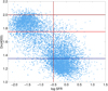 |
Fig. 1. Star formation rate (logSFR) versus Dn(4000) index for galaxies with Mr = −18.30. Horizontal lines show Dn(4000) limits for galaxies with stellar populations of different ages, 1.35, 1.75, and 2.0 (see text for details), and the vertical line shows the limit logSFR = −0.5 that separates star-forming and quenched galaxies. |
3. Methods
3.1. Spherical collapse model
We applied the spherical collapse model to describe the evolution of galaxy clusters as collapsing spherical shells. Evolution of galaxy clusters in these models can be described using several important epochs with characteristic density contrasts. In an expanding ΛCDM universe, all the densities and density contrasts depend on redshift. In the local Universe (z = 0) characteristic density contrasts for cosmological parameters applied in this paper are as follows. Density contrast for virialisation is Δρvir = 217, turnaround density contrast Δρta = 13.1, and density contrast at present for the objects that will collapse in the future (future collapse) is ΔρFC = 8.73. The density contrast ΔρZG = 5.41 corresponds to so-called zero gravity (ZG), at which the radial peculiar velocity component of the test particle velocity equals the Hubble expansion and the gravitational attraction of the system and its expansion are equal. We describe the spherical collapse model and its characteristic epochs with their density contrasts calculations as a function of redshift and other parameters in detail in Appendix A.
Undoubtedly, applying the spherical collapse model is an approximation only as nearly all real galactic systems are non-spherical. However, as demonstrated by Korkidis et al. (2020), comparing results of N-body simulations with the spherical collapse model calculations, this model also characterises the evolution of non-spherical systems (galaxy clusters) rather well. Thus, this justifies approximation in our analysis.
We defined the turnaround region around a cluster as the region at which border the “observed” density contrast is equal to the density contrast of turnaround, Δρta. Under the “observed” we mean the densities we calculated from the masses around clusters based on the dynamical masses of clusters and groups. Based on this definition, we found the radius and mass within the turnaround region, Rta and Mta (see also Einasto 2025, about the masses of superclusters). Also, we found the radius and mass around clusters within the virialisation region, Rvir and Mvir using density contrast Δρvir, and within the future collapse region, RFC and MFC using density contrast ΔρFC. We used these data to predict the future evolution of clusters and the whole superclusters.
For a spherical volume, the ratio of the density to the mean density (overdensity), Δρ = ρ/ρm, at different redshifts can be calculated as (see Eq. (A.6))
 (1)
(1)
where Ωm0 is the matter density parameter at present.
Using Eq. (1) we can calculate the relation between the mass and radius of an overdensity at various density contrasts and redshifts. For the mass within a sphere of influence, the density contrast in Eq. (1) corresponds to the density contrast, Δρinf, determined in this study. In Fig. 2 we show the mass–radius relation calculated using the cosmological parameters used in our study. In this figure, different lines show the mass versus radius of a spherical shell for a series of density contrasts (the turnaround, future collapse, and zero gravity), and for the density contrasts at the borders of the spheres of influence, Δρinf, as shown in this study.
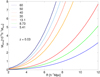 |
Fig. 2. Mass–radius relation from the spherical collapse model. Different lines correspond to the masses for different density contrasts, Δρ (Eq. (1)). Lines M60 − M30 correspond to the density contrasts, Δρinf, at the borders of the spheres of influence as found for clusters. Lines M13.1, M8.73, and M5.41 corresponds to the turnaround, future collapse, and zero gravity density contrasts. All lines are calculated for the redshift z = 0.03. |
3.2. Substructure of clusters
We searched for possible substructure of rich clusters in two ways. First, we applied the package mclust for multidimensional normal mixture modelling, classification and clustering (Fraley 2006) from R statistical environment (Ihaka & Gentleman 1996)6. mclust package have been used to search for substructure in galaxy clusters in, for example, Einasto et al. (2012). This package studies a finite mixture of distributions, in which each component is taken to correspond to a different subgroup of the cluster. mclust finds for each datapoint the probability to belong to a component. The mean uncertainty for the full sample is a statistical estimate of the reliability of the results. As an input for mclust, we used the sky coordinates and line-of-sight velocities (calculated from their redshifts) of the cluster member galaxies. The best solution for the components was chosen using the Bayesian information criterion (BIC). The algorithm finds components, their membership and probabilities for galaxies to belong to a component simultaneously. Einasto et al. (2012) tested how the errors in line-of-sight velocities of galaxies affect the reliability of the results of mclust. They applied test in which they shifted randomly the peculiar velocities of galaxies; these random shifts were chosen from a Gaussian distribution with the dispersion equal to the velocity dispersion of galaxies in a cluster. Such tests were performed 1000 times. The number of the components found by mclust remained unchanged, demonstrating that the results are robust against such errors. Second, we compared the substructure obtained in this way with partner clusters from WH24m catalogue (Wen et al. 2024).
3.3. Projected phase space diagram and various infall regions
In the PPS diagram we plotted line-of-sight velocities of galaxies with respect to the cluster mean velocity versus the projected clustercentric distance of galaxies. Simulations show that in this diagram, galaxies at small projected clustercentric distance form an early infall population with infall times τearly > 1 Gyr. The early infall region approximately corresponds to the virialised part of the clusters. Galaxies at large projected clustercentric distance form late infall populations with τlate < 1 Gyr (Oman et al. 2013; Muzzin et al. 2014; Haines et al. 2015; Costa et al. 2024). Borders of these infall regions can be approximately found as follows (Oman et al. 2013):
 (2)
(2)
where v are the velocities of the galaxies, σcl is the velocity dispersion of galaxies in the cluster, Dc is the projected clustercentric distance of galaxies, and Rvir is the cluster virial radius. Galaxies at small clustercentric distances may have been infallen at redshifts z ≥ 1, as suggested by ages of stellar populations of the brightest cluster galaxies (Einasto et al. 2022a).
Gravitational radius of clusters, Rg, is taken from Tempel et al. (2014a). This is the radius used in the scalar virial theorem (Binney & Tremaine 2008, Eq. (4.2.49a)) and it should not be confused with the cosmological virial radius (Binney & Tremaine 2008, Eq. (9.66)). We used the projected phase space diagram to determine regions of late infall of galaxies with characteristic radius Rcl. In the PPS diagram Rcl is marked by a small minimum in the clustercentric distance distributions of galaxies (Einasto et al. 2020, 2021). Usually Rcl is called the splashback radius–radius, at which the density profile of a cluster changes, and the slope of the correlation function of galaxies also changes, which is a signature of the crossover from galaxy correlations within a cluster to correlations in small groups in filaments between clusters (Einasto 1991; More et al. 2015; Haines et al. 2015; Rhee et al. 2017). At this radius outer (infalling) components and substructures reach the main component (main cluster) and galaxy orbits change (More et al. 2015). The value of this radius and how it is related to the other radii of the cluster depends on the structure and dynamical history of the cluster, and different probes may give different values for this radius (More et al. 2015; Lebeau et al. 2024). As we did not have data on galaxy orbits in our study, we called this radius as cluster radius Rcl. This radius approximately borders the late infall region of the cluster. We applied Eq. (2) with Rcl to show a late infall time region in the PPS diagram. Another radius which characterises clusters is their maximum size on the sky, Rmax, provided in Tempel et al. (2014a).
The border of the sphere of influence of groups is marked by another small minimum in the galaxy distribution around clusters in the PPS diagram. It defines the radius of the spheres of influence, Rinf (Einasto et al. 2020, 2021). Within the sphere of influence, galaxies and groups are falling into clusters. This is what Fong & Han (2021) proposed to call the depletion radius. We calculated the distribution of mass around clusters as the sum of masses of the main cluster and groups in these regions and used it to calculate the mass within the region of influence, Minf, and corresponding density contrast, Δρinf. With spherical collapse model and Δρinf we found at which redshifts regions of influence were at turnaround, and when in the future these regions will virialise.
3.4. Connectivity of clusters
The 3D connectivity of clusters is defined as the number of galaxy filaments, C = Nfil, connected to a cluster (Colombi et al. 2000; Codis et al. 2018). However, detecting filaments around clusters using observational data may be complicated due to the sometimes messy structures surrounding clusters (e.g. extended substructures) and infalling galaxies and groups. Elongated groups and also elongated substructures of clusters may be (mis)classified as short filaments. In order to determine the connectivity of clusters, we used Bisous filaments, as described above, and excluded very short filaments with a length of Flen < 3 h−1 Mpc, as they are less reliable. We note that galaxies are considered filament members if their distance to the nearest filament axis is Dfil ≤ 0.5 h−1 Mpc. We defined long filaments as filaments with a length of  Mpc and short filaments as those with a length of
  Mpc. We found the total number of filaments,
  , and the number of long filaments,
  , for each cluster within the region of influence of a cluster. This approach was used to determine the connectivity of the richest clusters in the A2142 and the Corona Borealis superclusters in Einasto et al. (2020, 2021). We compared our results with those obtained by Malavasi et al. (2020), who used the Discrete Persistent Structure Extractor (DisPerSe) to extract filaments in the Coma supercluster region, and with those by HyeongHan et al. (2024), who studied intracluster filaments in the Coma cluster.
4. Results
We present the results of our analysis in this section. We start with the overall analysis of the luminosity-density field and galaxy and group content of the region under study. Then we analyse the substructure and connectivity of clusters. Next, we determine different infall regions of clusters with their characteristic radii and calculate the density contrasts around clusters based on the mass distribution. Then we analyse the galaxy content in clusters, in their regions of influence, and in superclusters and low-density regions around clusters, and we analyse the relation between masses of clusters and masses embedded in their regions of influence and turnaround.
4.1. Structure of the Coma and Leo superclusters
We used the luminosity-density field to determine supercluster borders and to separate galaxies, groups, and clusters in superclusters and in surrounding low-density regions. Figure 3 (upper panel) shows the sky distribution of groups in our sample in a sky area covering the Coma and the Leo superclusters. We see that the luminous groups are mostly located in supercluster regions with D8 > 5.0, together with very poor groups and single galaxies. This figure shows also, that while in the environment of A1656 and A1185 galaxy filaments are dominating, the environment of A1367 is rich in galaxy groups (see also Seth & Raychaudhury 2020, who discussed groups surrounding this cluster). Cluster environments were also discussed in the early study of the Coma supercluster (Gregory & Thompson 1978). There is a minimum in the group and galaxy distribution around each cluster at distances ≈8 − 10 h−1 Mpc. We shall discuss this in Sect. 5.
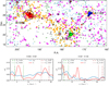 |
Fig. 3. Upper panel: Sky distribution of groups (filled circles and crosses) and single galaxies (empty circles) in the region of the Coma and the Leo superclusters. Colours of symbols show groups in different global luminosity-density regions (orange D8 ≥ 5, blue 5 > D8 ≥ 1.5, and grey crosses D8 < 1.5). To avoid strong projections, we only plot single galaxies in superclusters (D8 ≥ 5). Filament member galaxies in groups are shown with magenta x-s and single galaxies with green x-s. Violet stars show members of long filaments with length |

Figure 3 shows that there is a quite clear filament connecting clusters A1656 and A1367. The clusters A1367 and A1185 are separated by low-density environment (blue symbols, and the lack of orange symbols between these clusters, Fig. 3). In the lower panels of Fig. 3 we show the linear density of galaxies versus their distances along the straight line connecting the clusters from A1656 to A1367 (left panel), and from A1367 to A1185 (right panel). We can notice that along the filaments, there are minima in the grouped galaxy distributions at distances ≈4 h−1 Mpc and ≈8 h−1 Mpc from each cluster.
4.2. Substructure and connectivity of clusters
To analyse the substructure of clusters, we found components of each cluster, using SDSS data and applying mclust. The number of components, Ncomp, and their properties are given in Table B.2. Independently, we found from WH24m partner cluster systems (Table B.1). The number of components, Ncomp, and the number of partners using WH24 and WH24m data, Npart, as well as other main parameters of the three main clusters are given in Table 2.
Properties of clusters in superclusters.
In Fig. 4, for each cluster, we show the distribution of galaxies in the cluster and around it in the sky plane (upper row), as well as the PPS diagram (middle row), and the density contrast δρ, calculated from the distribution of mass around clusters, versus clustercentric distance R (lower row). In the sky plane plot in upper panels, we show the border of the sphere of influence and mark partner clusters from the WH24m catalogue.
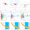 |
Fig. 4. Upper row: Distribution of galaxies in clusters and in their environment in the plane of the sky. Left: A1656. Middle: A1367. Right: A1185. Symbols of different colours show galaxies in different components of the cluster: the redder the colour, the higher the median values of the Dn(4000) index of galaxies are in a component. Black crosses show galaxies of short filaments ( |


Table 2 and Fig. 4 show that all clusters in our study have substructure. The Coma cluster, A1656, consists of two main components (components 1 and 3 in Table 2) and three smaller components in the outer parts of the cluster (Fig. 4) (see also Durret et al. 1997, where two main components were discussed). Component 4 may be an endpoint of an infalling filament (HyeongHan et al. 2024). Interestingly, A1656 is often considered as a typical relaxed cluster (Boselli & Gavazzi 2006; Seth & Raychaudhury 2020). In contrast and in agreement with our results, other studies found that the Coma cluster represents a typical cluster with substructure (see Biviano 1998, for an early review). In agreement with this, Caretta et al. (2023) showed that A1656 has a significant substructure in which massive component (central cluster) is accreting smaller groups. A recent analysis of intracluster light in the A1656 suggests that even the main component of this cluster has subclumps, and the brightest galaxies in it are in the process of merging (Jiménez-Teja et al. 2025).
The cluster A1367 is known as a dynamically active cluster with two components and a merger shock (see Deshev et al. 2022; Ge et al. 2019, and references therein). Our analysis revealed these components, and a short filament in the direction of merger shock described by Ge et al. (2019).
In cluster A1185, usually the galaxy NGC 3550 is considered as the main (brightest) galaxy (West et al. 2011). However, in Tempel et al. (2014a), this is the second brightest galaxy in this cluster. The brightest galaxy and the second brightest galaxy both lie in the main component of the cluster and are offset with its X-ray centre (West et al. 2011). Main component of A1185 hosts also interacting galaxy NGC 3561 (Arp 105), a signature of dynamical activity (West et al. 2022). One component, identified with the WH24 cluster J110718.2+283140, maybe a terminal part of a long filament. Another WH24 cluster, J111203.3+273523, may represent a group, falling into cluster along filament which points towards A1367.
Our results of substructure analysis are in a good agreement with partner systems from the WH24m catalogue. Main clusters in the WH24m partner systems can be identified with the richest components among substructures, and partners with poor components. There are two exceptions. WH24 cluster J115242.6 + 2037534, one of the partner clusters of the cluster A1367, corresponds in our catalogue to a short filament within it’s sphere of influence. Poor cluster J114612.2 + 202330 is not among A1367 partners, probably due to a redshift difference and strict definition of partner clusters in WH24m. When we compared the masses of clusters, the sum of the masses of partner cluster systems from WH24m agreed well with the cluster masses from SDSS data. However, our analysis did not detect fine details in each component of clusters, as, for example, in Jiménez-Teja et al. (2025) for the Coma cluster. This comparison shows that, in fact, in different studies the same structures have been found, but, due to the different definitions, these systems may have been identified differently (short filament versus partner cluster versus cluster component). Also, the use of mclust have its limitations. It assumes Gaussianity, and it performs better with a large number of galaxies in a cluster (Ribeiro et al. 2013). However, the good agreement between different substructure and partner cluster analysis shows that mclust gives reliable results.
Connectivity of clusters. To determine the connectivity of clusters, we first analysed the PPS diagram of clusters (Fig. 4, middle row) in order to find the radius of the sphere of influence of clusters, Rinf. The border of the sphere of influence is marked by a small minimum in the galaxy distribution around clusters in the PPS diagrams. The values of Rinf are given in Table 2. The radius of influence for A1656,  Mpc agrees well with the radius which was determined by Benisty et al. (2025) as a distance from the cluster centre, at which the velocities of galaxies change. Also other clusters have approximately the same radii of influence, Rinf ≈ 3.8 h−1 Mpc.
The median value of the ratio of radii Rcl and Rmax in our study is Rcl/Rmax ≈ 0.71. Gouin et al. (2022) showed that the parameter which characterises the shape of clusters seems to change at relative radius reff ≈ 0.75, which approximately corresponds to our ratio Rcl/Rmax. As Rcl is close to the radius at which galaxy orbits change, the change in the shape parameter in Gouin et al. (2022) may be related to that.
Next, we identified galaxy filaments within Rinf, which defines the 3D connectivity of clusters. We provide in Table 2 the number of all filaments Nfilall, and the number of long filaments,  , connected to a given cluster. For comparison with previous work, we show in Table 2 also data on the characteristic radii, masses, and connectivity for the rich clusters in the Corona Borealis and in the A2142 superclusters. Data on these clusters (A2065, A2061, A2089, Gr2064 in the Corona Borealis supercluster, and A2142 in the SCl A2142) in Table 2 are from Einasto et al. (2020, 2021). We see that clusters in the Coma and Leo superclusters have lower connectivity than clusters in the Corona Borealis supercluster. Especially high is the connectivity of the cluster of the highest mass, A2065.
In this study we considered galaxies as filament members if their distance to the nearest filament axis Dfil ≤ 0.5 h−1 Mpc. Typical width of filaments is approximately 1 h−1 Mpc, as also found from IllustrisTNG simulations for the present epoch by Yang et al. (2025) (1 − 1.5 h−1 Mpc in their study where they use DisPerSE filament finder to identify filaments). Einasto et al. (2020) analyse how the use of different distances to the nearest filament axis Dfil affects the detection of filaments and, consequently, the connectivity of clusters. The use of large Dfil may merge close filaments near clusters (as in the case of filaments at east side of the Coma cluster), decreasing the value of connectivity of clusters. Also, the use of larger Dfil may make filaments wider and sparser, or even create false filaments from sparse distribution of galaxies and groups. The exact change in filament properties depends on the configuration of galaxies near clusters. Einasto et al. (2020) also analyse how the use of larger Dfil may affect the connectivity of groups outside clusters, in low-density environment. We refer to Einasto et al. (2020), Sect. 4 for the details of this analysis.
Malavasi et al. (2020) use the DisPerSE filament finder to detect long filaments around A1656. In this study three long filaments are detected. This is less than in our study; the difference is related to the different methods to define filaments. The structure at approximately RA ≈ 196° and Dec ≈ 26° in Fig. 4 (upper left panel) is identified as a filament in our study, but it is not among filaments in Malavasi et al. (2020) (see their Fig. 2).
We note that components in A1656 agree well with the positions of intracluster filaments found by HyeongHan et al. (2024) in A1656, based on weak lensing analysis of Hyper Suprime-Cam imaging data (their N and W filaments). One short filament in our study coincides with their SE filament. Moreover, Keshet et al. (2017) reported a discovery of a virial shock region around A1656 with radius of about 5 Mpc. The borders of this shock region approximately agree with the borders of the region of influence around this cluster. Mirakhor & Walker (2020) detected an extended X-ray emission in the direction of the filament from A1656 towards A1367, seen also in Fig. 4. Another shock is related to components 4 and 5. Filament end W was also reported by Chen et al. (2025).
Two long filaments connected to the cluster A1367 have been noted earlier by Cortese et al. (2004) and West & Blakeslee (2000). Cortese et al. (2004) described A1367 as dynamically young cluster of two components, as also found in our analysis.
4.3. Density contrasts, characteristic radii, and masses
In Fig. 4 (lower panels) we present the density contrast Δρ for each cluster in our study, calculated using the distribution of mass around clusters. In this figure the blue area shows the turnaround region, and light blue area corresponds to the future collapse region. From Fig. 4 we can find the characteristic density contrast at the borders of the regions of influence and the mass embedded within these regions, Δρinf, and Minf. Using Fig. 4 we also found radii and embedded masses for the characteristic epochs of the spherical collapse model, namely, turnaround, future collapse, and zero gravity (with corresponding radii and masses Rta, RFC, Rzg, and Mta, MFC, Mzg). The values of these radii, masses, and density contrasts (for the spheres of influence) are given in Table 2.
For A1656, characteristic radii can be compared with those presented in Fig. 2 by Teerikorpi et al. (2015), which presents the so-called Λ significance diagram – another way to show the relation between the mass (density contrast) and the radius of an object. For the A1656 cluster Teerikorpi et al. (2015) present several regions. At small radius (R ≈ 1.4) the figure shows the location of the A1656 cluster itself, larger radius (R ≈ 4.8) corresponds to the region of influence around A1656, in a good agreement with our estimate. The largest radius for A1656 is R ≈ 14 – approximately the radius of the zero gravity region around the cluster.
4.4. Galaxy content
Next, we analysed the star formation properties of galaxies in clusters and around them, using star formation rates log(SFR) and Dn(4000) index. Distribution of these parameters are given in Fig. 5 separately for galaxies in clusters and in the regions of influence of clusters, in high-density regions (excluding clusters) and in low-density regions, in filaments and outside of filaments. Galaxies are considered as filament members if their distance to the nearest filament axis Dfil ≤ 0.5 h−1 Mpc, otherwise they are located outside filaments. For these subsamples we show in Table 3 the median values of log(SFR) and Dn(4000). Galaxy content of components in clusters is given in Table B.2. Calculations presented in Table B.2 have been made using absolute magnitude limit Mr ≤ −18.3, in order to compare magnitude-limited samples.
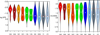 |
Fig. 5. Star formation rate logSFR (left) and Dn(4000) index for galaxies in clusters, in the regions of influence (i) of clusters, in the high-density regions (D85, excluding clusters; global luminosity-density D8 ≥ 5), and in the low-density regions (D805, D8 < 5 in the units of mean luminosity-density) of our sample and filament members (with distance from the nearest filament axis Dfil < = 0.5 h−1 Mpc) and non-member galaxies (Dfil > 0.5 h−1 Mpc). Different samples are marked in the figure. We only considered filaments with length Lfil ≥ 3 h−1 Mpc as more reliable. The horizontal line in the left panel corresponds to logSFR = −0.5, and lines in the right panel correspond to Dn(4000) = 1.55, 1.75, and 2.0. |
Galaxy content of clusters and areas around them.
Table 3 and Fig. 5 show, as expected, that clusters and superclusters, in general, contain a higher percentage of quenched galaxies with no active star formation than regions around them, and low-density regions between superclusters. We tested the statistical significance of the difference in galaxy populations between high and low global density environments and between filament member galaxies and those not in filaments using the Kolmogorov-Smirnov (KS) test. We considered that if p ≤ 0.01 then the differences between distributions are highly significant. We did not apply the KS test when samples were too small, with fewer than 20 galaxies (Ribeiro et al. 2013; Einasto et al. 2024).
First, we compared galaxy populations in clusters A1656, A1367, and A1185, and found that these are different with very high significance, with p < 0.01 between all cluster pairs. Galaxies with the oldest stellar populations, Dn(4000)≥2.0, reside in A1656 cluster, and also in the environments of clusters. In A1656 and A1367 the percentage of quenched galaxies in clusters is higher than in their regions of influence. In A1656, the main component and third component (orange symbols in Fig. 4) embed the highest percentage of passive galaxies with old stellar populations among different components in this cluster. KS test tells that galaxy populations in A1656 and its region of influence are different with high significance level (p < 0.01). The cluster A1367 and especially its region of influence, has a higher percentage of star-forming galaxies; populations are different with a high significance level, p < 0.01. This was also noted by Rakos et al. (2007). In A1367 the main component has a higher percentage of passive galaxies with old stellar populations. The second component has a higher percentage of star-forming galaxies. The SFRs in the first and second component of A1367 are different with high significance (p < 0.01), but the difference between the Dn(4000) index values is not significant, with p < 0.11. This is because of almost similar percentage of galaxies with very old stellar populations in these two components.
For A1185 we see the opposite – the cluster itself has a higher percentage of star-forming galaxies than its surrounding region. According to the SFR, the star formation properties of galaxies in the cluster and in it’s sphere of influence are different with high significance (p < 0.01). However, the significance of differences is low if we consider the Dn(4000) index, with p < 0.3. This mainly comes from the low percentage of quenched galaxies in its main component (Table B.2), and it is related to a lower percentage of galaxies with very old stellar populations, Dn(4000)≥1.75 in this cluster. As noted in Sect. 4.2, this component shows various signatures of ongoing dynamical activity, as the decentering of its brightest galaxy and the presence of interacting galaxies (West et al. 2011, 2022). This may result in excess star formation in this component. In the third component of A1185 the percentage of passive galaxies with old stellar populations is also very low.
The results on galaxy properties in clusters and their regions of influence for A1656 and A1367 agree with the finding by Einasto et al. (2021) in their study of the Corona Borealis (CB) supercluster. They find a certain concordance between galaxy clusters and their close environment: clusters with a lower fraction of quiescent galaxies also have a lower fraction of such galaxies among infalling groups and filaments. Clusters A1367 and Gr2064 in the CB also have the same total number of filaments connected to them,  (Table 2). However, A1656 also has six filaments and a larger number of substructures while having a lower percentage of star-forming galaxies in its neighbourhood. The cluster A1185 has an even lower percentage of quiescent galaxies in the main component of the cluster than in its sphere of influence. This shows a large variety in galaxy populations of clusters and around them.
The difference between galaxy populations in high (excluding rich clusters) and low global density environments is also highly significant. It is interesting to note that galaxies with the oldest stellar populations (Dn(4000)≥2.0) reside also in the low-density environments populated mostly by poor groups and single galaxies. We tested whether this result changes if we change the threshold density D8 used to separate high and low global density regions. We compared galaxy content of high and low global density environments using global density range 4 ≤ D8 ≤ 6. This changes the number of galaxies in high- and low global density environments, and also changes the median values of Dn(4000) index and logSFR, but this change is very small, less than 1%, and statistical significance of the differences remains very high, with p ≪ 0.01. This agrees well with the much more detailed comparison of the galaxy content of various global environments in Einasto et al. (2022a).
However, galaxy populations in filaments and outside of filaments are statistically similar. This similarity does not change if we change the criteria of filament membership (distance of a galaxy to the filament axis, to be a member of a filament). Such similarity was noticed also in Perez et al. (2024) who analysed the effect of filaments of galaxies from IllustrisTNG simulations. One reason for this similarity may be that filaments may cross regions of various global densities. Long filaments may extend from high-density cores of superclusters to low-density regions (voids) and may be populated differently along the filaments (see also corresponding discussion in Einasto et al. 2020).
We emphasise that in total, quiescent galaxies outside clusters in the low global luminosity-density regions outnumber almost ten times the same population in three richest clusters in our study (Fig. 5 and Table 3). Even in the low-density region among grouped and single galaxies 25% have very old stellar populations, an indicator of preprocessing of these galaxies far from rich clusters. The same was shown in Einasto et al. (2022a), who discussed the possible mechanisms of galaxy quenching in poor groups and in those galaxies which do not belong to any group in low-density environment.
In Fig. 6, we compare cluster masses, substructure, connectivity, and galaxy content, and show the trend that clusters with a higher mass also have a larger number of filaments connected to them, and a larger number of components. The cluster with the highest mass in our sample, A2065 in the Corona Borealis supercluster (ID = 4), has the largest total number of filaments connected to it. From Table 2 we see that it also has the highest mass embedded in it’s sphere of influence. Corresponding values for A1656 (cluster 1 in Fig. 6) are close to those for the cluster A2142 (cluster 8). Our mass estimates approximately agree with those from the constrained simulations of the local Universe (Hernández-Martínez et al. 2024). Figure 6 also shows variety in cluster properties – one of the clusters with a higher percentage of star-forming galaxies (A1367, cluster 2) has small values of substructure and connectivity, while A1185 (cluster 3) has a large number of components, but three long filaments connected to it.
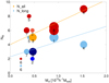 |
Fig. 6. Number of filaments connected to a cluster, Nfil, versus the cluster mass, Mcl. Symbol sizes are proportional to the number of components in a cluster, Ncomp. The numbers are order numbers of a cluster from Table 2. Red symbols show the number of all filaments, and blue symbols the number of long filaments with |

4.5. Scaling relations for masses and radii of clusters
To find possible scaling relations between different masses of clusters and their environment, and between various radii of clusters, we present in Fig. 7 the masses of clusters Mcl versus mass in the regions of influence (Minf, left panel), and in the turnaround region (Mta, right panel). In Fig. 7 symbols sizes are proportional to the total number of filaments connected to a cluster, and colours indicate the percentage of quiescent galaxies in a cluster, as determined in Sect. 4.4. In Fig. 8 we show the relations between various radii of clusters and their environment; the cluster gravitational radii Rg and radii Rcl, Rinf, and Rta. Figure 7 shows tight correlation between cluster masses and the mass embedded in the region of influence and in the turnaround region. For all clusters the mass in their spheres of influence is Minf ≈ 1.6Mcl + 0.2, for all masses and connectivities. The turnaround mass Mta ≈ 2.2Mcl + 0.3.
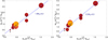 |
Fig. 7. Scaling relations between the cluster mass, Mcl, and the mass embedded in the sphere of influence (Minf, left panel) and turnaround mass (Mta, right panel). Symbol sizes are proportional to the number of all filaments connected to a cluster, Nfil. Dark red symbols show clusters with a high percentage of quiescent galaxies, and light red and orange symbols show clusters with a lower percentage of quiescent galaxies (light red – A1367, and orange – A1185). Dashed lines show 1σ errors of the linear fit, and error bars show mass errors (Table 2). Numbers are order numbers of a cluster from Table 2. |
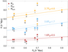 |
Fig. 8. Scaling relations between the cluster gravitational radii, Rg, and cluster radii, Rcl (dark red); the radii of the regions of influence, Rinf (blue); and the radii of the turnaround regions, Rta (orange). Parameters of the linear scaling relations are given in the figure. Dashed lines show 1σ errors of linear fit, and error bars show radii errors. Numbers are order numbers of a cluster from Table 2. |
The scaling relations between different mass estimates of clusters were presented by Maraboli et al. (2025). In comparison with our work, there are important differences. Maraboli et al. (2025) determined the scaling relations between cluster masses M200 (the radius within region in which the mean density is 200 times the critical density of the universe), and MHern, the mass calculated using Hernquist profile (see Maraboli et al. 2025, for details), in other words, within the same dark matter halo. They detected linear scaling relations in the case of clusters without significant substructure. In our calculations regions of influence and turnaround regions correspond to the environment of clusters beyond the cluster dark matter haloes, and all clusters have substructure. The sizes of the regions of influence and turnaround regions are larger for more massive clusters which represent deep potential wells, and embed larger number of galaxies, groups, and filaments (Figs. 6 and 8). Groups near more massive clusters may also be of higher mass than groups near less massive clusters (environmental enhancement of galaxy groups, see, for example, Einasto et al. 2003). Therefore, positive correlations between masses are expected. However, it is interesting that the scatter in the relations between masses is so small, as the structures surrounding each cluster are different. The regions of influence around A1656 and A1185 are dominated by filaments while A1367 is surrounded by a large number of galaxy groups. The scatter of the scaling relations between radii in Fig. 8 is larger. Thus, before making conclusions we need to study larger sample of clusters. Our findings extend the scaling relations between different mass estimates of galaxy clusters to a larger radii than in previous studies.
5. Discussion
We showed that all three clusters in our sample have substructure, with 2–5 components and up to six filaments connected to them. Substructures found in our study agree well with parent clusters from the DESI cluster catalogue. More massive clusters have a higher number of components and higher connectivity, but the scatter is large. We also found the characteristic radii of clusters, Rcl, Rinf, Rta, and RFC, and the distribution of mass around clusters, which gives us the density contrast at the borders of the regions of influence of clusters, Δρinf = 50 − 60, as well as the sizes and masses of turnaround and future collapse regions. According to the star formation properties, A1656 and its region of influence contain the lowest percentage of star-forming galaxies among clusters under study. Especially high is the percentage of star-forming galaxies in cluster A1185, and in the region of influence of the cluster A1367. This percentage is also higher than in and around comparison clusters from the A2142 and the Corona Borealis superclusters. The scaling relation between cluster masses and the mass embedded in the region of influence and in the turnaround region has a very small scatter. Below, we discuss what our results tell us about the evolution of clusters.
5.1. Evolution of clusters: From formation to future
Cluster formation and virialisation. Simulations show that the formation of structures in the universe – galaxies, groups, and clusters is modulated by the combination of density waves. Galaxies and their systems can form in the density field where positive phases combine so that the combination of small- and large-scale density perturbations is sufficiently high (Einasto et al. 2011; Suhhonenko et al. 2011; Peebles 2021). The richest clusters form at the highest combined density peaks and grow by the infall of galaxies and groups along filaments. Based on zoom-in simulations of galaxy clusters (THE THREEHUNDRED project) Kuchner et al. (2022) estimated that up to 45% of galaxies fall into clusters along filaments. Chiang et al. (2013) estimate that protoclusters of Coma-like clusters with present-day mass Mz0 ≈ 1.0 × 10¹⁵ M⊙ increased their masses ten times during evolution from z = 2 (approximately 10 Gyr ago) to the present day. An effective radius of such clusters was Reff ≈ 7 − 8 h−1 Mpc at redshift z = 2. The masses of protoclusters with present-day mass Mz0 ≈ 0.5 × 10¹⁵ M⊙ (as A1367 and A1185) were approximately five times lower at z = 2, and their effective radius at z = 2 was Reff ≈ 5 h−1 Mpc. The actual growth of a particular protocluster depends on its surrounding structures.
Based on the density contrast evolution, the turnaround of the virialised central parts of clusters in our study with Δρ = Δρvir at present occured approximately at redshift z ≈ 0.7 (Fig. A.1) or when the age of the Universe was 7.5 Gyr. At that time, in A1656 galaxies with Dn(4000)≥2 already stopped forming stars. The percentage of such galaxies is the highest in the main component and in the third component of A1656. Such galaxies formed their stellar populations approximately 10 Gy ago, at redshift z ≈ 1.5 − 2. Other components have lower Dn(4000) and higher star formation rate values. The W direction from A1656 with its substructures and filaments pointing towards A1367 is probably the main direction for cluster growth for A1656. This interpretation agrees with the position of components and filaments in the PPS diagram (Fig. 4), as well as with the predictions from simulations and observations of the evolution of protoclusters, and the brightest cluster galaxies (Chiang et al. 2013; Lin et al. 2025; Hewitt et al. 2025).
In other clusters the percentage of star-forming galaxies is higher than in A1656 at present, and we may assume that it was higher also at redshifts z ≈ 0.7. The PPS diagram shows that the second component of A1367 lies in the late infall region. Figure 3 shows that in the surroundings of A1367 there is more galaxy groups than in the neighbourhood of A1656, with the higher percentage of star-forming galaxies in its region of influence than in the cluster or in the region of influence of A1656 (groups and galaxy populations in A1367 were also described in Seth & Raychaudhury 2020). We may assume that with its lower mass, the infall of surrounding groups has been slower in this cluster, which leads to longer timescales of cluster formation and group merger times in comparison with A1656, and to ongoing star formation activity in the cluster and its region of influence.
In the cluster A1185 the main component has lower percentage of passive galaxies with old stellar populations than another, smaller component. This may be related to the clumpy distribution of passive galaxies in the main component, a signature of dynamical activity in this component, seen also in the X-ray maps of the cluster. This activity enhances the star formation in galaxies (Mahdavi et al. 1996; Hoessel et al. 1985; West et al. 2011; Hernández-Fernández et al. 2012). However, Jiménez-Teja et al. (2025) determined many small subclumps also in the A1656, while the percentage of star-forming galaxies in Coma is lower than in A1185. The third component in A1185 with the highest percentage of star-forming galaxies and the youngest stellar populations may represent a small group falling into the cluster for the first time.
Clusters, especially A1656 have galaxies with the oldest stellar populations in their main component (early infall region). Recently, Hewitt et al. (2025) showed that in the GOGREEN and GCLASS surveys at redshifts 0.8 < z < 1.5, cores of clusters have higher fraction of quiescent galaxies than outskirts of clusters, in agreement with findings in our study. Hewitt et al. (2025) suggest that in the early infall (core) region of clusters galaxy quenching is mostly related to accelerated mass dependent quenching of galaxies in protoclusters, while in late infall (non-core) regions quenching is better described by environmental, mass-independent processes of infalling galaxy populations.
Regions of influence. Present-day regions of influence were next regions around clusters to reach turnaround and to start collapse. We found that the radii of the regions of influence of clusters are Rinf ≈ 4 h−1 Mpc, and the density contrast at the borders of these regions is Δρinf ≈ 40 − 70.
The relation between the present (at z = 0.02 − 0.03) density contrast and the turnaround redshift zta at a specific redshift is presented in Fig. A.4. We can see that if the present density contrast at the borders of regions of influence is Δρinf ≈ 40 − 70, then the turnaround should have occurred at redshifts zta ≈ 0.47 − 0.57. In the Corona Borealis and A2142 superclusters (at z = 0.07 − 0.09) Δρinf ≈ 30 − 40, which means that regions of influence of rich clusters in these superclusters were at the turnaround and started to collapse at redshift zta ≈ 0.48 − 0.55 (Einasto et al. 2020, 2021). Figure A.2 suggests that if the turnaround occurred at the redshifts zta ≈ 0.4 − 0.6 then such regions will virialise in the future, approximately after 3.3 Gyr from now (at the age of the Universe ≈17.1 Gyr, corresponding to z ≈ −0.2 in Fig. A.2).
Turnaround and future evolution. The current radii of turnaround regions around A1656 and A1367 are Rta ≈ 7 − 8 h−1 Mpc, and the radii of the future collapse regions are RFC ≈ 8 − 10 h−1 Mpc (Table 2). Mass, embedded in these regions are of order of Mta ≈ (1.5 − 2.5)×1015 M⊙, and MFC ≈ (2.0 − 2.5)×1015 M⊙. Based on Fig. A.2, we can predict that the regions at turnaround now (at z = 0) will be virialised after 10 Gyrs from now, at the age of the Universe ≈22.9 Gyr.
Figure 3 shows that the distance between these clusters is approximately 24 h−1 Mpc, with the minimum in the distribution of groups between clusters approximately at 9 h−1 Mpc from A1656. Although at these distances there is a maximum of single galaxy distribution, these galaxies do not contribute much to the total mass7. Therefore, even if we underestimate the mass and size of the turnaround region around A1656 and around A1367, it is still unlikely that A1656 and A1367 will merge in the future to form massive, collapsing supercluster core. This conclusion is somewhat different made by Zúñiga et al. (2024), who proposed that the clusters A1656 and A1367 perhaps may collapse in the future into one system. To merge in the future, the size of the future collapse regions around clusters A1656 and A1367 should be at least 12 − 13 h−1 Mpc, so that these regions overlap and can collapse together. This means that the mass in these regions should be at least M = 5 − 10 × 1015 M⊙ (see Fig. 2). This mass is in the same order as the mass of a collapsing core of the Shapley supercluster which embeds 11 rich clusters or in the Corona Borealis supercluster (Chon et al. 2015; Einasto et al. 2021; Aghanim et al. 2024). Also, this leads to 5–10 times higher mass-to-light ratio of these clusters, up to M/L ≈ 3000 − 4000, which is highly unlikely (see also discussion of mass-to-light ratios and the size of collapsing regions in Einasto et al. 2015, 2022b).
The cluster A1185 is far away from other clusters in our sample, and it will collapse separately. Its future collapse size and mass are of order of  Mpc and
  (Table 2). It is interesting to note that although the environments of both A1656 and A1185 are dominated by filaments, their evolution and present dynamical state is different, as suggests the galaxy content of these clusters and their regions of influence.
Einasto et al. (2014) and Cohen et al. (2017) showed that in superclusters where galaxy clusters are connected by a large number of filaments (superclusters of (multi)spider type) the fraction of star-forming galaxies is higher, and clusters have more substructures than in superclusters with simple structure (small number of filaments between clusters). In agreement with this, Ko et al. (2024) found that clusters with larger number of FoF-connected structures in their neighbourhood tend to have higher fraction of star-forming galaxies at redshifts approximately 0.4 and higher, up to redshifts z ≈ 0.9. At still higher redshifts clusters have high fraction of star-forming galaxies no matter how large is the number of connected structures around them - the properties of clusters in the IllustrisTNG simulation at redshift z = 1 are quite homogeneous.
Clusters grow by infall of matter from surroundings, and simulations enable their evolution to be followed back up to very high redshifts (Chiang et al. 2013, 2017). Masses of massive clusters have grown more than twice since redshift z = 1 (Kim et al. 2015). The properties of clusters in the IllustrisTNG simulation at redshift z = 1 are quite homogeneous (Ko et al. 2024). We found that the properties of clusters in our sample show large variety in substructure, connectivity, and galaxy content. We may assume that the origin of this variety is related to the evolution of clusters from z = 1 to the present. This shows the need for a further study of a large sample of clusters both from observations and simulations.
5.2. Cluster masses, connectivity, and substructure
In Fig. 6 we showed large variety in the connectivity of clusters of the same mass, or, in other words, clusters of the same connectivity and/or the same number of components may have very different masses. We can compare this result with the masses, dynamical state, and connectivity of clusters in IllustrisTNG300 simulations by Gouin et al. (2021). Gouin et al. (2021) found that at the same cluster mass, relaxed clusters from Illustris TNG300 simulations have lower connectivity determined using T-ReX filament finder, than unrelaxed clusters. We get the same trend, but there are differences. In our study, the scatter in connectivity values is larger than found in Gouin et al. (2021), and we apply Bisous filament finder (Tempel et al. 2014b, 2016). We found that the connectivity values, when using all filaments, are C = 2 − 9, and for long filaments connectivity C = 1 − 5, versus C = 3 − 4 in Gouin et al. 2021). Also, in Gouin et al. (2021) connectivity is higher for clusters with substructure (nonregular clusters). In our study all clusters have substructure, and masses of clusters are higher than in IllustrisTNG300 simulations. Partly the differences between the studies come from different definition of filaments and connectivity.
Theoretical predictions in Codis et al. (2018) showed that the connectivity of massive haloes is approximately 5. The number of long filaments in our study is lower than that, but the number of all filaments, on average, agree with this prediction. These examples show the same trends between masses, connectivity, and substructure using different estimates of the substructure and connectivity of clusters, but also emphasise that direct comparison of different studies may not be straightforward, as the results depend on the methods applied to determine connectivity and substructure. Also, if filaments are connected to a cluster from both sides, then in our study these are considered as different filaments, but in some other studies – as the same filament (see also Codis et al. 2018). The comparison of cluster masses, substructure and connectivity from observations and simulations is yet to be done in the future studies.
5.3. Large-scale environment of galaxies
In the supercluster outskirt regions (in superclusters, excluding rich clusters, thus in poor groups and clusters and among single galaxies), there is approximately ten times more quiescent galaxies than in clusters. In the whole superclusters (D8 > 5) the percentage of quiescent galaxies is higher than in low-density regions between superclusters (D8 < 5), with median values Dn(4000)med ≈ 1.52 in superclusters and Dn(4000)med ≈ 1.40 in low-density region between superclusters (see Table 3, for D8 > 5 and D8 < 5, respectively). Singh et al. (2025) found that quiescent galaxies at z = 3 are similar in various environments (protoclusters, filaments). They concluded that quenching mechanisms are likely driven by similar physical processes independent of their environments. This is the same conclusion as in Einasto et al. (2022a, 2024), Bidaran et al. (2025): quenching occurs in all environments, and in low-density environments the number of quenched galaxies is even larger than in rich clusters (Table 3, the last line).
Gouin et al. (2020) analysed galaxy content in clusters and filaments from Magneticum hydrodynamical simulations and found that passive galaxies trace filamentary pattern around clusters better than star-forming galaxies. This suggests that quenching mechanisms are related to processes within galaxies and their dark matter haloes or in their immediate neighbourhood (infalling filaments), like AGN feedback, morphological quenching, detachment of primordial filaments and others are more important in quenching galaxy formation in galaxies in low-density environments than environmental processes related to galaxy mergers and interactions in high-density environments. Galaxy quenching via detachment of primordial filaments (Cosmic Web Detachment, CWD) have been described in detail by Aragon Calvo et al. (2019). They show that the accretion of gas into galaxies from primordial gaseous filaments around them stops when these filaments are disrupted due to the influence of other galaxies, infall to groups and so on. This process leads to the end of star formation in galaxies, combining several mechanisms such as starvation, harassment, and strangulation. Einasto et al. (2022a) suggested that the CWD may be one of the mechanisms of galaxy quenching in global low-density environments. Song et al. (2021) apply DisPerSE filament finder to galaxies from HORIZON-AGN simulations and find that the star formation in galaxies is suppressed at the edge of filaments. They suggest that gas transfer to haloes becomes less efficient closer to filaments which may explain the higher percentage of passive galaxies in filaments.
6. Summary
We have studied the substructure, connectivity, galaxy content, characteristic radii, and mass distribution of the richest clusters in the Coma and Leo superclusters, A1656, A1367, and A1185 and their environments. We used these data to analyse the timeline of the formation and evolution of these clusters and superclusters. We summarise our results as follows:
-
(1)
The clusters under study have two to four components and a connectivity of C = 5 − 6. The highest percentage of quiescent galaxies is in A1656, and the lowest is in A1185. In the region of influence of A1185, the percentage of quiescent galaxies is higher than in the cluster itself, due to the high percentage of quiescent galaxies in an infalling group.
-
(2)
Outside of the clusters, in the superclusters and in the low-density region between superclusters with no rich groups, approximately 25% of the galaxies are quiescent. They are mostly located in small groups, or they are single galaxies. As the richest clusters contain only a small fraction of all galaxies, quiescent galaxies outside of rich clusters outnumber such galaxies in clusters by at least a factor of ten.
-
(3)
The radii of the regions of influence of all clusters is Rinf ≈ 4 h−1 Mpc, and the density contrast is Δρinf ≈ 50 − 60. This suggests that the turnaround of the regions of influence occurred, and the collapse started at redshifts of z ≈ 0.4 − 0.5. The turnaround regions around clusters will virialise in the future, approximately 9–10 Gyr from now.
-
(4)
In the future, these clusters will not merge; they will form separate collapsing structures with radii of RFC ≈ 8 − 10 h−1 Mpc and masses of MFC ≈ (1.8 − 2.5)×1015 M⊙.
-
(5)
Our study extends the known scaling relations between cluster masses to larger distances from clusters. The scaling relations between the cluster mass and the mass embedded in the regions of influence and in the turnaround regions have a very small scatter.
The properties of clusters (their substructure, connectivity, and galaxy content) vary strongly, which suggests that they each experienced a different evolution. Our findings indicate the self-similarity of mass distribution around clusters and extend the scaling relations between different mass estimates of galaxy clusters to a larger radii than in previous studies. Ko et al. (2024) showed that at redshift z = 1 and higher, the properties of clusters in the IllustrisTNG300 simulation are quite homogeneous. The scatter of cluster connectivities in the IllustrisTNG simulation is lower than found in our study Gouin et al. (2021). According to Horizon Run 4 simulations, the clusters with a present-day mass of order of M ≈ ×1015 M⊙ have gathered half of their masses between redshifts 1 and 0 (Kim et al. 2015). This rises the question as to whether the large variety of present-day cluster properties appeared during the evolution in last 7–8 Gyrs or if there is a difference between observations and simulations. These questions point to the significance of conducting future studies that analyse a large number of clusters, their environments, connectivity, and galaxy properties simultaneously using both observations and large simulations. Such studies will involve the use of data from present and forthcoming surveys such as the J-PAS survey (Benitez et al. 2014) and especially the forthcoming 4MOST survey (de Jong et al. 2019; Driver et al. 2019; Taylor et al. 2023) and data from multiwavelength studies. In the future, the 4MOST cluster survey will increase the number of clusters and supercluster regions that can be studied in detail, including the environment of clusters up to 5R200 (Sifón et al. 2025).
For example, Einasto et al. (2021) found that approximately 5% of the mass of the Corona Borealis supercluster comes from single galaxies.
Mixing: Fundamental frequencies of nearby orbits differ a little, and thus their positions in phase space start to differ more and more, ultimately reaching a quasi-stationary state. In the case of chaotic orbits, these orbits move away exponentially from each other and end up filling all the available space. Violent relaxation: A nonstationary potential changes particle energies so that their energy distribution expands. Landau damping: An exchange of energies between the perturbation waves and particles causes an increase of kinetic energies of particles due to the damping of waves.
Acknowledgments
We thank the referee for valuable comments and suggestions which helped us to improve the paper. We thank Hyeong Han Kim and Mirt Gramann for discussions. This work was supported by the Estonian Ministry of Education and Research (grant TK202, “Foundations of the Universe”), Estonian Research Council grant PRG1006, by Estonian Research Council grants PRG2172 and PRG2159, and the European Union’s Horizon Europe research and innovation programme (EXCOSM, grant No. 101159513). This work has also been supported by ICRAnet through a professorship for Jaan Einasto. We applied in this study R statistical environment (Ihaka & Gentleman 1996), and Julia language Bezanson et al. (2017).
References
- Aghanim, N., Tuominen, T., Bonjean, V., et al. 2024, A&A, 689, A332 [NASA ADS] [CrossRef] [EDP Sciences] [Google Scholar]
- Ahn, C. P., Alexandroff, R., Allende Prieto, C., et al. 2014, ApJS, 211, 17 [NASA ADS] [CrossRef] [Google Scholar]
- Aihara, H., Allende Prieto, C., An, D., et al. 2011, ApJS, 193, 29 [NASA ADS] [CrossRef] [Google Scholar]
- Aragon Calvo, M. A., Neyrinck, M. C., & Silk, J. 2019, Open J. Astrophys., 2, 7 [CrossRef] [Google Scholar]
- Bahé, Y. M., McCarthy, I. G., Balogh, M. L., & Font, A. S. 2013, MNRAS, 430, 3017 [Google Scholar]
- Balogh, M. L., Morris, S. L., Yee, H. K. C., Carlberg, R. G., & Ellingson, E. 1999, ApJ, 527, 54 [Google Scholar]
- Benisty, D., Wagner, J., Haridasu, S., & Salucci, P. 2025, arXiv e-prints [arXiv:2504.04135] [Google Scholar]
- Benitez, N., Dupke, R., Moles, M., et al. 2014, arXiv e-prints [arXiv:1403.5237] [Google Scholar]
- Bezanson, J., Edelman, A., Karpinski, S., & Shah, V. B. 2017, SIAM Rev., 59, 65 [Google Scholar]
- Bidaran, B., Pérez, I., Sánchez-Menguiano, L., et al. 2025, A&A, 693, L16 [NASA ADS] [CrossRef] [EDP Sciences] [Google Scholar]
- Binney, J., & Tremaine, S. 2008, Galactic Dynamics: Second Edition (Princeton University Press) [Google Scholar]
- Biviano, A. 1998, in Untangling Coma Berenices: A New Vision of an Old Cluster, eds. A. Mazure, F. Casoli, F. Durret, & D. Gerbal, 1 [Google Scholar]
- Boldrini, P., & Laigle, C. 2025, A&A, 700, A182 [NASA ADS] [CrossRef] [EDP Sciences] [Google Scholar]
- Boselli, A., & Gavazzi, G. 2006, PASP, 118, 517 [Google Scholar]
- Brinchmann, J., Charlot, S., White, S. D. M., et al. 2004, MNRAS, 351, 1151 [Google Scholar]
- Caretta, C. A., Andernach, H., Chow-Martínez, M., et al. 2023, Rev. Mex. Astron. Astrofis., 59, 345 [Google Scholar]
- Chang, C.-C., Lee, W., & Ng, K.-W. 2018, Phys. Dark Universe, 19, 12 [Google Scholar]
- Chen, X.-B., Wang, K., Huang, Y.-Y., et al. 2025, ApJ, 978, L47 [Google Scholar]
- Chiang, Y.-K., Overzier, R., & Gebhardt, K. 2013, ApJ, 779, 127 [Google Scholar]
- Chiang, Y.-K., Overzier, R. A., Gebhardt, K., & Henriques, B. 2017, ApJ, 844, L23 [Google Scholar]
- Chon, G., Böhringer, H., & Zaroubi, S. 2015, A&A, 575, L14 [NASA ADS] [CrossRef] [EDP Sciences] [Google Scholar]
- Codis, S., Pogosyan, D., & Pichon, C. 2018, MNRAS, 479, 973 [Google Scholar]
- Cohen, S. A., Hickox, R. C., Wegner, G. A., Einasto, M., & Vennik, J. 2017, ApJ, 835, 56 [Google Scholar]
- Colombi, S., Pogosyan, D., & Souradeep, T. 2000, Phys. Rev. Lett., 85, 5515 [Google Scholar]
- Cortese, L., Gavazzi, G., Boselli, A., Iglesias-Paramo, J., & Carrasco, L. 2004, A&A, 425, 429 [NASA ADS] [CrossRef] [EDP Sciences] [Google Scholar]
- Costa, A. P., Ribeiro, A. L. B., de Carvalho, R. R., & Benavides, J. A. 2024, MNRAS, 535, 1348 [Google Scholar]
- de Jong, R. S., Agertz, O., Berbel, A. A., et al. 2019, Messenger, 175, 3 [Google Scholar]
- Deshev, B., Taylor, R., Minchin, R., Scott, T. C., & Brinks, E. 2022, A&A, 665, A155 [NASA ADS] [CrossRef] [EDP Sciences] [Google Scholar]
- DESI Collaboration (Adame, A. G., et al.) 2024, AJ, 168, 58 [NASA ADS] [CrossRef] [Google Scholar]
- Driver, S. P., Liske, J., Davies, L. J. M., et al. 2019, Messenger, 175, 46 [Google Scholar]
- Durret, F., Biviano, A., Gerbal, D., et al. 1997, Astrophys. Lett. Commun., 36, 97 [Google Scholar]
- Einasto, M. 1991, MNRAS, 252, 261 [NASA ADS] [CrossRef] [Google Scholar]
- Einasto, M. 2025, Universe, 11, 167 [Google Scholar]
- Einasto, M., Einasto, J., Müller, V., Heinämäki, P., & Tucker, D. L. 2003, A&A, 401, 851 [NASA ADS] [CrossRef] [EDP Sciences] [Google Scholar]
- Einasto, J., Suhhonenko, I., Hütsi, G., et al. 2011, A&A, 534, A128 [NASA ADS] [CrossRef] [EDP Sciences] [Google Scholar]
- Einasto, M., Vennik, J., Nurmi, P., et al. 2012, A&A, 540, A123 [NASA ADS] [CrossRef] [EDP Sciences] [Google Scholar]
- Einasto, M., Lietzen, H., Tempel, E., et al. 2014, A&A, 562, A87 [NASA ADS] [CrossRef] [EDP Sciences] [Google Scholar]
- Einasto, M., Gramann, M., Saar, E., et al. 2015, A&A, 580, A69 [NASA ADS] [CrossRef] [EDP Sciences] [Google Scholar]
- Einasto, M., Deshev, B., Tenjes, P., et al. 2020, A&A, 641, A172 [NASA ADS] [CrossRef] [EDP Sciences] [Google Scholar]
- Einasto, M., Kipper, R., Tenjes, P., et al. 2021, A&A, 649, A51 [NASA ADS] [CrossRef] [EDP Sciences] [Google Scholar]
- Einasto, M., Kipper, R., Tenjes, P., et al. 2022a, A&A, 668, A69 [NASA ADS] [CrossRef] [EDP Sciences] [Google Scholar]
- Einasto, M., Tenjes, P., Gramann, M., et al. 2022b, A&A, 666, A52 [NASA ADS] [CrossRef] [EDP Sciences] [Google Scholar]
- Einasto, M., Einasto, J., Tenjes, P., et al. 2024, A&A, 681, A91 [NASA ADS] [CrossRef] [EDP Sciences] [Google Scholar]
- Fong, M., & Han, J. 2021, MNRAS, 503, 4250 [NASA ADS] [CrossRef] [Google Scholar]
- Fraley, C. 2006, Technical Report, Dep. of Statistics, University of Washington, 504, 1 [Google Scholar]
- Ge, C., Sun, M., Liu, R.-Y., et al. 2019, MNRAS, 486, L36 [NASA ADS] [CrossRef] [Google Scholar]
- Gouin, C., Aghanim, N., Bonjean, V., & Douspis, M. 2020, A&A, 635, A195 [NASA ADS] [CrossRef] [EDP Sciences] [Google Scholar]
- Gouin, C., Bonnaire, T., & Aghanim, N. 2021, A&A, 651, A56 [NASA ADS] [CrossRef] [EDP Sciences] [Google Scholar]
- Gouin, C., Gallo, S., & Aghanim, N. 2022, A&A, 664, A198 [NASA ADS] [CrossRef] [EDP Sciences] [Google Scholar]
- Gramann, M., Einasto, M., Heinämäki, P., et al. 2015, A&A, 581, A135 [NASA ADS] [CrossRef] [EDP Sciences] [Google Scholar]
- Gregory, S. A., & Thompson, L. A. 1978, ApJ, 222, 784 [NASA ADS] [CrossRef] [Google Scholar]
- Haines, C. P., Pereira, M. J., Smith, G. P., et al. 2015, ApJ, 806, 101 [NASA ADS] [CrossRef] [Google Scholar]
- Haines, C. P., Iovino, A., Krywult, J., et al. 2017, A&A, 605, A4 [NASA ADS] [CrossRef] [EDP Sciences] [Google Scholar]
- Hernández-Fernández, J. D., Iglesias-Páramo, J., & Vílchez, J. M. 2012, ApJS, 199, 22 [CrossRef] [Google Scholar]
- Hernández-Martínez, E., Dolag, K., Seidel, B., et al. 2024, A&A, 687, A253 [NASA ADS] [CrossRef] [EDP Sciences] [Google Scholar]
- Hewitt, G., Sarron, F., Balogh, M. L., et al. 2025, MNRAS, 541, 409 [Google Scholar]
- Hoessel, J. G., Borne, K. D., & Schneider, D. P. 1985, ApJ, 293, 94 [Google Scholar]
- Huchra, J. P., & Geller, M. J. 1982, ApJ, 257, 423 [NASA ADS] [CrossRef] [Google Scholar]
- HyeongHan, K., Jee, M. J., Cha, S., & Cho, H. 2024, Nat. Astron., 8, 377 [NASA ADS] [CrossRef] [Google Scholar]
- Ihaka, R., & Gentleman, R. 1996, J. Comput. Graphical Stat., 5, 299 [Google Scholar]
- Jiménez-Teja, Y., Román, J., HyeongHan, K., et al. 2025, A&A, 694, A216 [NASA ADS] [CrossRef] [EDP Sciences] [Google Scholar]
- Jõeveer, M., Einasto, J., & Tago, E. 1978, MNRAS, 185, 357 [Google Scholar]
- Kauffmann, G., Heckman, T. M., White, S. D. M., et al. 2003, MNRAS, 341, 33 [Google Scholar]
- Keshet, U., Kushnir, D., Loeb, A., & Waxman, E. 2017, ApJ, 845, 24 [NASA ADS] [CrossRef] [Google Scholar]
- Kim, J., Park, C., L’Huillier, B., & Hong, S. E. 2015, J. Korean Astron. Soc., 48, 213 [Google Scholar]
- Ko, E., Im, M., Lee, S.-K., & Laigle, C. 2024, ApJ, 976, 154 [Google Scholar]
- Kofman, L. A., & Shandarin, S. F. 1988, Nature, 334, 129 [NASA ADS] [CrossRef] [Google Scholar]
- Komatsu, E., Smith, K. M., Dunkley, J., et al. 2011, ApJS, 192, 18 [Google Scholar]
- Korkidis, G., Pavlidou, V., Tassis, K., et al. 2020, A&A, 639, A122 [EDP Sciences] [Google Scholar]
- Kravtsov, A. V., & Borgani, S. 2012, ARA&A, 50, 353 [Google Scholar]
- Kuchner, U., Haggar, R., Aragón-Salamanca, A., et al. 2022, MNRAS, 510, 581 [Google Scholar]
- Lahav, O., Lilje, P. B., Primack, J. R., & Rees, M. J. 1991, MNRAS, 251, 128 [Google Scholar]
- Lebeau, T., Ettori, S., Aghanim, N., & Sorce, J. G. 2024, A&A, 689, A19 [NASA ADS] [CrossRef] [EDP Sciences] [Google Scholar]
- Lee, S., & Ng, K.-W. 2010, JCAP, 2010, 028 [Google Scholar]
- Liivamägi, L. J., Tempel, E., & Saar, E. 2012, A&A, 539, A80 [Google Scholar]
- Lin, Y.-T., Chen, K.-F., Chen, T.-C., Chuang, C.-Y., & Oguri, M. 2025, AJ, 169, 285 [Google Scholar]
- Mahdavi, A., Geller, M. J., Fabricant, D. G., et al. 1996, AJ, 111, 64 [Google Scholar]
- Malavasi, N., Aghanim, N., Tanimura, H., Bonjean, V., & Douspis, M. 2020, A&A, 634, A30 [NASA ADS] [CrossRef] [EDP Sciences] [Google Scholar]
- Maor, I., & Lahav, O. 2005, JCAP, 2005, 003 [Google Scholar]
- Maraboli, E., Grillo, C., Bergamini, P., & Giocoli, C. 2025, A&A, 698, A272 [NASA ADS] [CrossRef] [EDP Sciences] [Google Scholar]
- Mirakhor, M. S., & Walker, S. A. 2020, MNRAS, 497, 3204 [Google Scholar]
- More, S., Diemer, B., & Kravtsov, A. V. 2015, ApJ, 810, 36 [Google Scholar]
- Muzzin, A., van der Burg, R. F. J., McGee, S. L., et al. 2014, ApJ, 796, 65 [Google Scholar]
- Oman, K. A., Hudson, M. J., & Behroozi, P. S. 2013, MNRAS, 431, 2307 [Google Scholar]
- Peebles, P. J. E. 1980, The Large-Scale Structure of the Universe (Princeton University Press) [Google Scholar]
- Peebles, P. J. E. 1984, ApJ, 284, 439 [Google Scholar]
- Peebles, P. J. E. 2021, arXiv e-prints [arXiv:2106.02672] [Google Scholar]
- Perez, N. R., Pereyra, L. A., Coldwell, G., et al. 2024, MNRAS, 534, 2228 [Google Scholar]
- Rakos, K., Schombert, J., & Odell, A. 2007, ApJ, 658, 929 [Google Scholar]
- Rhee, J., Smith, R., Choi, H., et al. 2017, ApJ, 843, 128 [Google Scholar]
- Ribeiro, A. L. B., de Carvalho, R. R., Trevisan, M., et al. 2013, MNRAS, 434, 784 [NASA ADS] [CrossRef] [Google Scholar]
- Seth, R., & Raychaudhury, S. 2020, MNRAS, 497, 466 [Google Scholar]
- Sifón, C., Finoguenov, A., Haines, C. P., et al. 2025, A&A, 697, A92 [NASA ADS] [CrossRef] [EDP Sciences] [Google Scholar]
- Singh, A., Guaita, L., Hibon, P., et al. 2025, A&A, 700, A68 [NASA ADS] [CrossRef] [EDP Sciences] [Google Scholar]
- Song, H., Laigle, C., Hwang, H. S., et al. 2021, MNRAS, 501, 4635 [NASA ADS] [CrossRef] [Google Scholar]
- Suhhonenko, I., Einasto, J., Liivamägi, L. J., et al. 2011, A&A, 531, A149 [NASA ADS] [CrossRef] [EDP Sciences] [Google Scholar]
- Taylor, E. N., Cluver, M., Bell, E., et al. 2023, Messenger, 190, 46 [Google Scholar]
- Teerikorpi, P., Heinämäki, P., Nurmi, P., et al. 2015, A&A, 577, A144 [NASA ADS] [CrossRef] [EDP Sciences] [Google Scholar]
- Tempel, E., Tamm, A., Gramann, M., et al. 2014a, A&A, 566, A1 [NASA ADS] [CrossRef] [EDP Sciences] [Google Scholar]
- Tempel, E., Stoica, R. S., Martínez, V. J., et al. 2014b, MNRAS, 438, 3465 [CrossRef] [Google Scholar]
- Tempel, E., Stoica, R. S., Kipper, R., & Saar, E. 2016, Astron. Comput., 16, 17 [NASA ADS] [CrossRef] [Google Scholar]
- Tremonti, C. A., Heckman, T. M., Kauffmann, G., et al. 2004, ApJ, 613, 898 [Google Scholar]
- Wang, P. 2006, ApJ, 640, 18 [Google Scholar]
- Wang, L., & Steinhardt, P. J. 1998, ApJ, 508, 483 [NASA ADS] [CrossRef] [Google Scholar]
- Wen, Z. L., & Han, J. L. 2024, ApJS, 272, 39 [NASA ADS] [CrossRef] [Google Scholar]
- Wen, Z. L., Han, J. L., & Yuan, Z. S. 2024, MNRAS, 532, 1849 [Google Scholar]
- West, M. J., & Blakeslee, J. P. 2000, ApJ, 543, L27 [NASA ADS] [CrossRef] [Google Scholar]
- West, M. J., Jordán, A., Blakeslee, J. P., et al. 2011, A&A, 528, A115 [NASA ADS] [CrossRef] [EDP Sciences] [Google Scholar]
- West, M. J., De Propris, R., & Gregg, M. D. 2022, Caught in the Act: The Hierarchical Formation of Abell 1185, HST Proposal. Cycle 30, ID. #17212 [Google Scholar]
- Yang, Q.-R., Zhu, W., Yu, G.-Y., et al. 2025, ApJ, 989, 187 [Google Scholar]
- Zeldovich, I. B., Einasto, J., & Shandarin, S. F. 1982, Nature, 300, 407 [Google Scholar]
- Zúñiga, J. M., Caretta, C. A., & Andernach, H. 2024, PASA, 41, e078 [Google Scholar]
Appendix A: Spherical collapse and virialisation model
Let us have a spherical overdensity Δρ ≡ ρ/ρm within a radius R, where ρ is the matter density in the volume, and ρm is the mean matter density. As the universe expands, the overdensity expands also. In principle, some matter falls to the overdensity, but it is not dominating, and usually, the mass of the overdensity is assumed to be constant (as we also do). The growth of masses are large at the formation stages of overdensities at very high redshifts (z > 20 − 30) but such high redshifts are beyond our analysis.
In overdensity regions, due to internal gravitation, expansion is slower than in the surrounding background. At a particular moment, the (slower) expansion may stop, and the region starts to contract. This is called a turnaround epoch. Depending on a value of the density contrast Δρ, the turnaround may occur in the past, present, or future or may not occur at all. We can calculate these ”critical” density contrasts for a given cosmological model.
Let us now fix our cosmological model. We assume an expanding ΛCDM universe. Cosmological parameters are taken from Komatsu et al. (2011): present matter density and dark energy density parameters Ωm0 = 0.27 and ΩΛ0 = 0.73, respectively. The Universe is assumed to be flat Ω = 1 with dark energy parameter ω = −1. In our cosmological model, we do not look at a very early time. Thus, we need not to consider radiation; the matter is only baryonic and dark matter. The density of the dark energy is assumed to be constant in space and time.
The time evolution of the matter density parameter is
 (A.1)
(A.1)
and of the Hubble function is
 (A.2)
(A.2)
The scale factor of the universe is designated as a. In following we use standard designations: overdensity is Δρ ≡ ρ/ρm, turnaround redshift is zta and overdensity at turnaround is Δρta. Density contrast at an arbitrary time is
 (A.3)
(A.3)
where x = a/ata and y = R/Rta are the scale factor and density contrast radius in turnaround units. Time, in this case, is also in dimensionless units
 (A.4)
(A.4)
(see, for example, Wang & Steinhardt 1998).
Differential equations describing the time evolution of x and y were derived by Wang & Steinhardt (1998, Appendix A) and Lee & Ng (2010). The analytical solution of the equation for x in the form of a hypergeometric function is well-known
![Mathematical equation: $$ \begin{aligned} \frac{2}{3} x^{3/2} F\left[ \frac{1}{2}, \frac{1}{2}, \frac{3}{2}, -\frac{x^3\rho _{\Lambda }}{\rho _{ta}} \right] = \tau . \end{aligned} $$](/articles/aa/full_html/2025/12/aa56023-25/aa56023-25-eq45.gif) (A.5)
(A.5)
Here F is the hypergeometric function. The solution of the equation for y can be written as an integral, with integration constants derived from the boundary conditions at the turnaround (Eqs. 2.13 and 2.20 in Lee & Ng (2010)). Parameter Δρta in these equations can be calculated then from the condition that y(0) = 0 for different zta values. We calculated corresponding integrals numerically and derived Δρta values. Although an analytical approximation formula was proposed by Lee & Ng (2010) we calculated more precise Δρta values ourselves.
In this way, for a fixed turnaround redshift zta we have corresponding density contrast Δρta and functions x(τ) and y(τ). Corresponding density contrasts as a function of τ (and thereafter of z) result directly from Eq. A.3. If density contrast is expressed relative to local matter density, then
 (A.6)
(A.6)
where M is in units of (h−1M⊙) and R in (h−1kpc).
Let us turn now to virialisation. In the spherical collapse model, after the overdensity starts to contract, the final stage is the collapsed structure with a theoretical radius of zero—a singularity. In real, there exist several relaxation processes such as mixing of orbits, violent relaxation, and Landau damping,8 allowing us to avoid the singularity. Thus, the final stage should be a virialised state. It is usually postulated that in the contracting stage, the virialised state (equilibrium) is reached at the radius from which the virial theorem holds. We also use this to define the virial radius and designate it as Rvir. Using the virial theorem, it can be shown that in the case of the EdS universe, the virial radius is Rvir = 0.5 Rta (see, for example, Lahav et al. 1991), giving the corresponding density contrast value 147 (instead of the usual value 178, derived by allowing the system to contract to singularity).
In the case of a nonzero cosmological constant (ρΛ = const), it is necessary to include also the dark energy terms to the virial theorem equation (Lahav et al. 1991; Wang & Steinhardt 1998). In this case (ρΛ = const), the dark energy does not virialise (only the matter does) but still acts as a background and contributes to gravitational potential. Potential energy is not a function of time and energy is conserved. Using again the variable y as Rvir = yvir Rta, it can be shown (see Maor & Lahav 2005; Wang 2006; Lee & Ng 2010) that the virial theorem gives us for y (or more precisely for yvir) the relation
 (A.7)
(A.7)
A similar equation was derived earlier by Lahav et al. (1991), Wang & Steinhardt (1998) but for pressure-less dark energy (ω = 0).
In the case of variable dark energy density (ρΛ ≠ const), virialisation is much more complicated. In this case, one should consider that the dark energy is in direct gravitational interaction with the matter (it is not a constant background any more), and its contribution to gravitational potential is more complicated. Energy is not conserved also. In most general form, this was studied by Maor & Lahav (2005) and Chang et al. (2018).
In the present paper, we assume a constant dark energy density as supported by current CMB data (ω = −1 within the errors). In calculations, we fixed first a turnaround redshift zta. This gives us ρta ≡ ρm(zta) = Ωm(zta)ρcr(zta) and we solved Eq. A.7 to find yvir and corresponding dimensionless time τvir from Eq. A.4. After that, we calculated xvir from Eq. A.5. The density contrast corresponding to virialisation
 (A.8)
(A.8)
Virialisation time (and thereafter redshift) can be calculated again from Eq. A.4. This is the density contrast at which the collapse stops (does not go to zero), and the overdensity is virialised due to the processes referred to above.
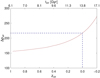 |
Fig. A.1. Density contrast at the virialised epoch Δρvir as a function of corresponding redshift zvir (time in upper axis). Negative redshift values must be interpreted as future cosmological times, shown in upper axis. |
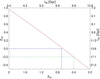 |
Fig. A.2. Relation between the turnaround and virial redshifts, zta and zvir. Negative redshift values must be interpreted as future cosmological times; timelines (corresponding age of the Universe) are shown in the right and upper axes. Systems which expansion have turned around at z = 0.4 (green dash-dotted line) or at z = 0.7 (blue dashed line) will be virialised in future (at 17.1 Gyr) or now (at 13.8 Gyr). |
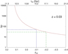 |
Fig. A.3. Density contrasts Δρ = ρ/ρm at z = 0.03 as a function of virialisation redshifts zvir. Negative redshift values must be interpreted as future cosmological times (timeline is shown in the upper axis). Green dot-dashed line corresponds to the density contrast Δρ = 30, and blue dashed line to the density contrast Δρ = 60, the range Δρinf found in this study. |
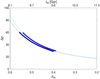 |
Fig. A.4. Density contrast Δρ at redshift z = 0.02 − 0.03 (upper and lower curves, respectively) for Ωm = 0.27, if the turnaround occurred at redshifts in the interval z = 0.6 − 0.2. Thicker parts of the curves correspond to the density contrasts Δρ = 30 − 60 (see Table 2 and Fig. A.3). |
Calculated density contrasts as a function of virialisation redshifts are shown in Fig. A.1. We see that the density contrast corresponding to the virialisation in the local Universe (z = 0) in the case of our used cosmological parameters is Δρvir = 217. This is similar to the density contrast used in literature and corresponds to the radius R200. However, we point out that the value is a function of redshift. For example, for systems at redshift z = 0.5, all regions with Δρ > 169 are virialised.
Virialisation redshift is related to turnaround redshift
 (A.9)
(A.9)
Although, in principle, xvir is also a function of zta this dependence is quite weak and from Fig. A.2 is is seen that Eq. A.9 is nearly a linear relation. Turnaround redshift corresponding to zvir = 0 is zta = 0.665.
Now we can calculate density contrasts ρ/ρm and densities ρ/ρm0 at any redshift, when the corresponding region is virialised at a certain redshift. In Fig. A.3 these values are given for a redshift z = 0.03, corresponding approximately to the clusters from the present paper, as a function of virialisation redshift. One can see that in the case of the present clusters at redshifts z ∼ 0.03, all regions with density contrasts ρ/ρm ≥ 210 have been virialised by the time we observe them. Corresponding value for the BOSS Great Wall is ρ/ρm ≥ 169. We also calculated the density contrasts at our clusters redshifts for cases in which the turnaround occurs at redshifts in the range of z = 0.6 − 0.2. In our calculations, we used formulae derived by Lee & Ng (2010). We show the results for Ωm = 0.27 in Fig. A.4.
Appendix B: Data on clusters: DESI clusters, and substructure
In this section we present data on clusters from WH24 catalogue (DESI data, Table B.1), and data on substructure of clusters, with identifications based on WH24m catalogue, and on HyeongHan et al. (2024) (Table B.2).
Data of rich galaxy clusters in the Coma and Leo superclusters identified in the WH24 cluster catalogue.
Substructure of clusters.
Appendix C: SDSS and DESI surveys
We are pleased to thank the SDSS survey team and DESI survey team for the publicly available data releases. Funding for the Sloan Digital Sky Survey (SDSS) and SDSS-II has been provided by the Alfred P. Sloan Foundation, the Participating Institutions, the National Science Foundation, the U.S. Department of Energy, the National Aeronautics and Space Administration, the Japanese Monbukagakusho, and the Max Planck Society, and the Higher Education Funding Council for England. The SDSS9 is managed by the Astrophysical Research Consortium (ARC) for the Participating Institutions. The Participating Institutions are the American Museum of Natural History, Astrophysical Institute Potsdam, University of Basel, University of Cambridge, Case Western Reserve University, The University of Chicago, Drexel University, Fermilab, the Institute for Advanced Study, the Japan Participation Group, The Johns Hopkins University, the Joint Institute for Nuclear Astrophysics, the Kavli Institute for Particle Astrophysics and Cosmology, the Korean Scientist Group, the Chinese Academy of Sciences (LAMOST), Los Alamos National Laboratory, the Max-Planck-Institute for Astronomy (MPIA), the Max-Planck-Institute for Astrophysics (MPA), New Mexico State University, Ohio State University, University of Pittsburgh, University of Portsmouth, Princeton University, the United States Naval Observatory, and the University of Washington.
The DESI Legacy Surveys consist of three individual and complementary projects: the Dark Energy Camera Legacy Survey (DECaLS; Proposal ID #2014B-0404; PIs: David Schlegel and Arjun Dey), the Beijing-Arizona Sky Survey (BASS; NOAO Prop. ID #2015A-0801; PIs: Zhou Xu and Xiaohui Fan), and the Mayall z-band Legacy Survey (MzLS; Prop. ID #2016A-0453; PI: Arjun Dey). DECaLS, BASS and MzLS together include data obtained, respectively, at the Blanco telescope, Cerro Tololo Inter-American Observatory, NSF’s NOIRLab; the Bok telescope, Steward Observatory, University of Arizona; and the Mayall telescope, Kitt Peak National Observatory, NOIRLab. Pipeline processing and analyses of the data were supported by NOIRLab and the Lawrence Berkeley National Laboratory (LBNL). The Legacy Surveys project is honored to be permitted to conduct astronomical research on Iolkam Du’ag (Kitt Peak), a mountain with particular significance to the Tohono O’odham Nation.
NOIRLab is operated by the Association of Universities for Research in Astronomy (AURA) under a cooperative agreement with the National Science Foundation. LBNL is managed by the Regents of the University of California under contract to the U.S. Department of Energy.
This project used data obtained with the Dark Energy Camera (DECam), which was constructed by the Dark Energy Survey (DES) collaboration. Funding for the DES Projects has been provided by the U.S. Department of Energy, the U.S. National Science Foundation, the Ministry of Science and Education of Spain, the Science and Technology Facilities Council of the United Kingdom, the Higher Education Funding Council for England, the National Center for Supercomputing Applications at the University of Illinois at Urbana-Champaign, the Kavli Institute of Cosmological Physics at the University of Chicago, Center for Cosmology and Astro-Particle Physics at the Ohio State University, the Mitchell Institute for Fundamental Physics and Astronomy at Texas A&M University, Financiadora de Estudos e Projetos, Fundacao Carlos Chagas Filho de Amparo, Financiadora de Estudos e Projetos, Fundacao Carlos Chagas Filho de Amparo a Pesquisa do Estado do Rio de Janeiro, Conselho Nacional de Desenvolvimento Cientifico e Tecnologico and the Ministerio da Ciencia, Tecnologia e Inovacao, the Deutsche Forschungsgemeinschaft and the Collaborating Institutions in the Dark Energy Survey. The Collaborating Institutions are Argonne National Laboratory, the University of California at Santa Cruz, the University of Cambridge, Centro de Investigaciones Energeticas, Medioambientales y Tecnologicas-Madrid, the University of Chicago, University College London, the DES-Brazil Consortium, the University of Edinburgh, the Eidgenossische Technische Hochschule (ETH) Zurich, Fermi National Accelerator Laboratory, the University of Illinois at Urbana-Champaign, the Institut de Ciencies de l’Espai (IEEC/CSIC), the Institut de Fisica d’Altes Energies, Lawrence Berkeley National Laboratory, the Ludwig Maximilians Universitat Munchen and the associated Excellence Cluster Universe, the University of Michigan, NSF’s NOIRLab, the University of Nottingham, the Ohio State University, the University of Pennsylvania, the University of Portsmouth, SLAC National Accelerator Laboratory, Stanford University, the University of Sussex, and Texas A&M University.
BASS is a key project of the Telescope Access Program (TAP), which has been funded by the National Astronomical Observatories of China, the Chinese Academy of Sciences (the Strategic Priority Research Program “The Emergence of Cosmological Structures” Grant # XDB09000000), and the Special Fund for Astronomy from the Ministry of Finance. The BASS is also supported by the External Cooperation Program of Chinese Academy of Sciences (Grant # 114A11KYSB20160057), and Chinese National Natural Science Foundation (Grant # 12120101003, # 11433005).
The Legacy Survey team makes use of data products from the Near-Earth Object Wide-field Infrared Survey Explorer (NEOWISE), which is a project of the Jet Propulsion Laboratory/California Institute of Technology. NEOWISE is funded by the National Aeronautics and Space Administration.
The Legacy Surveys imaging of the DESI footprint is supported by the Director, Office of Science, Office of High Energy Physics of the U.S. Department of Energy under Contract No. DE-AC02-05CH1123, by the National Energy Research Scientific Computing Center, a DOE Office of Science User Facility under the same contract; and by the U.S. National Science Foundation, Division of Astronomical Sciences under Contract No. AST-0950945 to NOAO.
All Tables
Data on rich galaxy clusters in the Coma and Leo superclusters based on SDSS DR10.
Data of rich galaxy clusters in the Coma and Leo superclusters identified in the WH24 cluster catalogue.
All Figures
|
Fig. 1. Star formation rate (logSFR) versus Dn(4000) index for galaxies with Mr = −18.30. Horizontal lines show Dn(4000) limits for galaxies with stellar populations of different ages, 1.35, 1.75, and 2.0 (see text for details), and the vertical line shows the limit logSFR = −0.5 that separates star-forming and quenched galaxies. |
| In the text | |
|
Fig. 2. Mass–radius relation from the spherical collapse model. Different lines correspond to the masses for different density contrasts, Δρ (Eq. (1)). Lines M60 − M30 correspond to the density contrasts, Δρinf, at the borders of the spheres of influence as found for clusters. Lines M13.1, M8.73, and M5.41 corresponds to the turnaround, future collapse, and zero gravity density contrasts. All lines are calculated for the redshift z = 0.03. |
| In the text | |
|
Fig. 3. Upper panel: Sky distribution of groups (filled circles and crosses) and single galaxies (empty circles) in the region of the Coma and the Leo superclusters. Colours of symbols show groups in different global luminosity-density regions (orange D8 ≥ 5, blue 5 > D8 ≥ 1.5, and grey crosses D8 < 1.5). To avoid strong projections, we only plot single galaxies in superclusters (D8 ≥ 5). Filament member galaxies in groups are shown with magenta x-s and single galaxies with green x-s. Violet stars show members of long filaments with length |
| In the text | |
|
Fig. 4. Upper row: Distribution of galaxies in clusters and in their environment in the plane of the sky. Left: A1656. Middle: A1367. Right: A1185. Symbols of different colours show galaxies in different components of the cluster: the redder the colour, the higher the median values of the Dn(4000) index of galaxies are in a component. Black crosses show galaxies of short filaments ( |
| In the text | |
|
Fig. 5. Star formation rate logSFR (left) and Dn(4000) index for galaxies in clusters, in the regions of influence (i) of clusters, in the high-density regions (D85, excluding clusters; global luminosity-density D8 ≥ 5), and in the low-density regions (D805, D8 < 5 in the units of mean luminosity-density) of our sample and filament members (with distance from the nearest filament axis Dfil < = 0.5 h−1 Mpc) and non-member galaxies (Dfil > 0.5 h−1 Mpc). Different samples are marked in the figure. We only considered filaments with length Lfil ≥ 3 h−1 Mpc as more reliable. The horizontal line in the left panel corresponds to logSFR = −0.5, and lines in the right panel correspond to Dn(4000) = 1.55, 1.75, and 2.0. |
| In the text | |
|
Fig. 6. Number of filaments connected to a cluster, Nfil, versus the cluster mass, Mcl. Symbol sizes are proportional to the number of components in a cluster, Ncomp. The numbers are order numbers of a cluster from Table 2. Red symbols show the number of all filaments, and blue symbols the number of long filaments with |
| In the text | |
|
Fig. 7. Scaling relations between the cluster mass, Mcl, and the mass embedded in the sphere of influence (Minf, left panel) and turnaround mass (Mta, right panel). Symbol sizes are proportional to the number of all filaments connected to a cluster, Nfil. Dark red symbols show clusters with a high percentage of quiescent galaxies, and light red and orange symbols show clusters with a lower percentage of quiescent galaxies (light red – A1367, and orange – A1185). Dashed lines show 1σ errors of the linear fit, and error bars show mass errors (Table 2). Numbers are order numbers of a cluster from Table 2. |
| In the text | |
|
Fig. 8. Scaling relations between the cluster gravitational radii, Rg, and cluster radii, Rcl (dark red); the radii of the regions of influence, Rinf (blue); and the radii of the turnaround regions, Rta (orange). Parameters of the linear scaling relations are given in the figure. Dashed lines show 1σ errors of linear fit, and error bars show radii errors. Numbers are order numbers of a cluster from Table 2. |
| In the text | |
|
Fig. A.1. Density contrast at the virialised epoch Δρvir as a function of corresponding redshift zvir (time in upper axis). Negative redshift values must be interpreted as future cosmological times, shown in upper axis. |
| In the text | |
|
Fig. A.2. Relation between the turnaround and virial redshifts, zta and zvir. Negative redshift values must be interpreted as future cosmological times; timelines (corresponding age of the Universe) are shown in the right and upper axes. Systems which expansion have turned around at z = 0.4 (green dash-dotted line) or at z = 0.7 (blue dashed line) will be virialised in future (at 17.1 Gyr) or now (at 13.8 Gyr). |
| In the text | |
|
Fig. A.3. Density contrasts Δρ = ρ/ρm at z = 0.03 as a function of virialisation redshifts zvir. Negative redshift values must be interpreted as future cosmological times (timeline is shown in the upper axis). Green dot-dashed line corresponds to the density contrast Δρ = 30, and blue dashed line to the density contrast Δρ = 60, the range Δρinf found in this study. |
| In the text | |
|
Fig. A.4. Density contrast Δρ at redshift z = 0.02 − 0.03 (upper and lower curves, respectively) for Ωm = 0.27, if the turnaround occurred at redshifts in the interval z = 0.6 − 0.2. Thicker parts of the curves correspond to the density contrasts Δρ = 30 − 60 (see Table 2 and Fig. A.3). |
| In the text | |
Current usage metrics show cumulative count of Article Views (full-text article views including HTML views, PDF and ePub downloads, according to the available data) and Abstracts Views on Vision4Press platform.
Data correspond to usage on the plateform after 2015. The current usage metrics is available 48-96 hours after online publication and is updated daily on week days.
Initial download of the metrics may take a while.