| Issue |
A&A
Volume 704, December 2025
|
|
|---|---|---|
| Article Number | A187 | |
| Number of page(s) | 9 | |
| Section | Extragalactic astronomy | |
| DOI | https://doi.org/10.1051/0004-6361/202556066 | |
| Published online | 09 December 2025 | |
Microhertz oscillations during the reformation of the inner disk-corona in the changing-look active galactic nucleus 1ES 1927+654
1
National Astronomical Observatories, Chinese Academy of Sciences, Beijing 100101, China
2
School of Astronomy and Space Science, University of Chinese Academy of Sciences, 19A Yuquan Road, Beijing 100049, China
3
Department of Physics, Anhui Normal University, Wuhu, Anhui 241002, China
4
Institute for Frontier in Astronomy and Astrophysics, Beijing Normal University, Beijing 102206, China
★ Corresponding authors: This email address is being protected from spambots. You need JavaScript enabled to view it.
; This email address is being protected from spambots. You need JavaScript enabled to view it.
Received:
24
June
2025
Accepted:
22
October
2025
Abstract
1ES 1927+654 has exhibited a spectroscopic changing-look transition following dramatic ultraviolet/optical (UV/optical) and X-ray variability in recent years. X-ray observations have revealed a rapid flux decline, when the hard X-ray power-law component disappeared, the soft thermal emission reached a minimum ∼150 days after the UV/optical peak, and both components reemerged with the source re-brightening. This extreme variability suggests the destruction and subsequent reformation of the inner disk and corona. Here, we report the discovery of quasiperiodic X-ray variability with a period of ∼12 days (significance > 3.2σ), which persisted for about 220 days, based on high-cadence monitoring during the inner disk-corona rebuilding phase. The signal is coherent with a very high quality factor of ∼58. We interpret this periodicity as a signature of radiation-pressure instability in the accretion disk, which occurs when the accretion rate and magnetic field strength reach appropriate values. This mechanism has been proposed as an explanation for quasiperiodic eruptions, a recently discovered intriguing phenomenon associated with galactic nuclei. Our findings provide a representative example of disk instability at moderate accretion rates. This phenomenon was long predicted by accretion theory, but rarely observed in active galactic nuclei (AGNs). Our research suggests that extreme events in AGNs, such as tidal disruption events, could serve as novel probes for testing and refining accretion theory.
Key words: galaxies: active / galaxies: individual: 1ES 1927+654 / galaxies: nuclei / galaxies: Seyfert
© The Authors 2025
 Open Access article, published by EDP Sciences, under the terms of the Creative Commons Attribution License (https://creativecommons.org/licenses/by/4.0), which permits unrestricted use, distribution, and reproduction in any medium, provided the original work is properly cited.
This article is published in open access under the Subscribe to Open model. This email address is being protected from spambots. You need JavaScript enabled to view it. to support open access publication.
1. Introduction
Active galactic nuclei (AGNs) are empirically classified into type 1 and type 2 according to their optical emission line widths. Type 1 AGNs show both broad and narrow emission lines in their spectra, while type 2 AGNs display only narrow lines. Some AGNs are known to transition from type 1 to type 2 or vice versa (Shappee et al. 2014; LaMassa et al. 2015; Trakhtenbrot et al. 2019). These objects are known as changing-look (CL) AGNs. One scenario interprets CL AGNs as being attributed to dramatic changes in the accretion rate (MacLeod et al. 2016; Sheng et al. 2017; Jana et al. 2025; Kang et al. 2025), with the continuum and broad lines expected to respond promptly, while narrow lines remain nearly unchanged. Such changes can be triggered by accretion disk instabilities or tidal disruption events (TDEs). A TDE occurs when a star passes too close to a supermassive black hole (SMBH) and is torn apart as tidal forces exceed the star’s self-gravity. Such events can rapidly enhance the accretion rate, producing luminous flares that typically peak in the soft X-ray and ultraviolet (UV) bands. TDEs were initially proposed as probes of otherwise quiescent black holes. Recent theoretical studies and simulations suggest that the TDE rate in AGNs is significantly higher than in quiescent galaxies (Karas & Šubr 2007; Kennedy et al. 2016). For instance, Chan et al. (2019, 2020) modeled TDE variability in AGNs with pre-existing accretion disks and showed that the fallback of bound stellar debris is modified by interactions with the ambient disk. As a result, the observed variability is expected to differ from canonical TDE light curves (Blanchard et al. 2017; Shu et al. 2018; Zhang et al. 2022a).
Recently, a new class of quasiperiodic X-ray eruptions (QPEs) has emerged from the vicinity of SMBHs in nearby, low-mass galactic nuclei (Miniutti et al. 2019; Giustini et al. 2020; Arcodia et al. 2021). Approximately ten QPEs hosts have been identified thus far (Jiang & Pan 2025 and references therein). They show peak luminosities ranging from 1042 to 1044 erg s−1 and recurrence times of T ∼ 2.5–100 hours. The mechanism behind these rare phenomena remains uncertain, but most models suggest that they involve accretion disks around SMBHs undergoing instabilities (Raj & Nixon 2021; Pan et al. 2022, 2023) or interacting with a stellar object in a close orbit (Xian et al. 2021; Franchini et al. 2023; Linial & Metzger 2023; Zhou et al. 2024). One hypothesis is that the accretion disk is created when the SMBH disrupts a passing star, implying that many QPEs could be preceded by observable TDEs. Since the discovery of QPEs, several observational properties have indeed related them to the aftermath of TDEs (Shu et al. 2018; Chakraborty et al. 2021; Sheng et al. 2021; Nicholl et al. 2024). Notably, a systematic study of optical spectra analysis of the host galaxies of known QPEs sources has identified that almost all QPEs host galaxies exhibit emission lines indicating the presence of AGNs (Wevers et al. 2022, 2024), linking QPEs to a fascinating class of phenomena associated with TDEs in AGNs (Gilbert et al. 2024; Jiang & Pan 2025).
1ES 1927+654 is a peculiar type-2 AGN that underwent a dramatic UV/optical outburst, followed by the emergence of broad optical emission lines (Trakhtenbrot et al. 2019; Ricci et al. 2020). High-cadence X-ray monitoring revealed extreme variability after the onset of the optical event: the X-ray flux experienced a rapid decline, during which the hard X-ray power-law component became undetectable and the soft thermal emission weakened, reaching a minimum luminosity of ∼1042 erg s−1 about 150 days after the peak. Subsequently, both spectral components reemerged over a period of ∼360 days as the source underwent re-brightening, with the luminosity ultimately rising above its pre-outburst level and reaching up to ∼2 × 1044 erg s−1 (Fig. 1, phase 1) (Trakhtenbrot et al. 2019; Ricci et al. 2020, 2021; Masterson et al. 2022, 2025). As the X-ray luminosity increased, a hot corona re-formed, giving rise to a very steep power-law component that dominated the 0.3–2 keV band. This extreme and coordinated variability has been interpreted by several scenarios, including accretion rate changes combined with a magnetically arrested disk, or a TDE followed by reformation of the inner disk-corona structure (Ricci et al. 2020, 2021; Masterson et al. 2022; Cao et al. 2023). Notably, during the re-brightening phase the X-ray luminosity varied by more than an order of magnitude on timescales shorter than one day (Ricci et al. 2020), a phenomenon rarely observed in AGNs. Following this transition, 1ES 1927+654 entered another atypical AGN phase, during which the coronal power-law index remained exceptionally soft relative to typical AGNs, while the soft excess became increasingly pronounced (Ghosh et al. 2023). In this stage, several unusual phenomena emerged, including transient X-ray quasiperiodic oscillations (QPOs) and transient jets, underscoring the extraordinary nature of 1ES 1927+654 (Masterson et al. 2025; Meyer et al. 2025). The QPOs exhibited evolving periods, shifting from 18 minutes to 7 minutes over two years, an evolution unprecedented in either SMBH QPOs or high-frequency QPOs in stellar-mass black holes. Although models such as orbital decay of a stellar-mass companion, coronal oscillations, and accretion disk instabilities have been considered (Masterson et al. 2025), each facing significant challenges in fully accounting for the observed behavior.
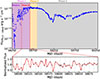 |
Fig. 1. Top panel: 0.3–10 keV NICER X-ray light curve for 1ES 1927+654 since May 2018 (blue). Following the methodology of Masterson et al. (2022), we divided the long-term X-ray light curve of 1ES 1927+654 into distinct phases. Phase 1 is characterized by a super-Eddington state with rapid fluctuations in both X-ray luminosity and spectral parameters. Phase 2 maintains a stable super-Eddington luminosity near its peak. Phase 3 exhibits a gradual decline in X-ray luminosity and spectral parameters, returning to levels comparable to those observed prior to the outburst. Phase 1 is divided into two equal segments and phase 1b is between the two vertical dashed red lines in phase 1. Bottom panel: Observation data in phase 1b plotted as black points after binning all observations within three-day intervals for visual clarity. To enhance the visibility of the periodic signal, we applied the logarithmic function f(x) = A ⋅ log(Bx + C)+D and removed the long-term trend, connecting the data and model points with a smoothed curve. Note: this approach is intended solely for visual illustration of periodicity. Dashed gray vertical lines denote a period of 11.6 days. |
In this work, we focus on the X-ray variability during the phase of inner disk-corona reformation. We detected another significant QPO in 1ES 1927+654 with a period of approximately 12 days, which could be driven by accretion disk instability. In Section 2, we describe the observations and data reduction procedures. In Section 3, we present a detailed analysis of the long-term X-ray light curve and our significance tests. In Section 4, we discuss the possible origin of the QPO.
2. Observations and data reduction
Neutron star Interior Composition Explorer (NICER; (Gendreau et al. 2012) started monitoring 1ES 1927+654 on 22 May 2018, with a typical cadence between observations of a few hours to a few days. We initiated our analysis by acquiring the publicly available level 1 data from the HEASARC archive1. The data were processed using the nicerl2 pipeline with the default screening criteria as outlined in the NICER data analysis guide2, version 2024-02-09_V012). This procedure yielded a set of good time intervals (GTIs), which are continuous observational segments ranging in duration from approximately 10 seconds to 2 230 seconds. NICER comprises 52 co-aligned focal plane modules (FPMs), which serve as independent detectors. Within each GTI, certain FPMs may exhibit anomalous behavior due to optical light loading, commonly referred to as being “hot”. We applied level 3 filtering to the background-subtracted light curves, adopting threshold count rates of two counts s−1 in the S0 band (0.2–0.3 keV) and 0.05 counts s−1 in the HBG band (13–15 keV) (Masterson et al. 2025). To further mitigate instrumental noise, we excluded data from detectors 14 and 34, which are known to exhibit elevated noise levels. Additionally, we identified and removed the “hot detectors” using an iterative sigma-clipping algorithm: any detector with a raw count rate in the E < 0.2 keV range exceeding the median by more than 4σ was excluded. A similar sigma-clipping procedure was used to filter out good time intervals (GTIs) with anomalously high background levels; specifically, any GTI with a 15–18 keV count rate exceeding the median for all GTIs by more than 4σ, as this energy band is dominated by background events. This data analysis closely follows the framework established in Masterson et al. (2022, 2025), Pasham et al. (2021, 2023, 2024a,b). As reported by Ricci et al. (2021), we also found that both the source and background exhibit significant variability in the NICER data. This is reflected in the presence of intervals where the source is barely distinguishable from the background, as well as segments where the signal-to-noise ratio (S/N) in the 0.3–2 keV band exceeds 1000. We further found that the low-significance intervals mostly correspond to very short GTIs. To minimize the influence of background fluctuations on our final results, we therefore excluded GTIs with durations shorter than 100 seconds. The source signal consistently exceeded the background level in the 0.3–2.0 keV energy range, which we therefore adopted for the majority of our light curve and spectral analysis. Overall, only the GTIs that remained valid after the above screening procedures were retained for subsequent analysis. Subsequent spectral modeling was carried out in XSPEC, employing the χ2 statistic.
3. Light-curve analysis and results
We first fitted each NICER observation using one of two spectral models, depending on whether a significant emission line around 1 keV was present (Masterson et al. 2022). The two models considered were: tbabs × ztbabs × (zbb + zpower) and tbabs × ztbabs × (zbb + zpower + zgauss). To assess the necessity of the additional Gaussian component, we compared the fit statistics between the two models. Specifically, we adopted the model including the Gaussian emission line only if its inclusion led to a reduction in the fit statistic of Δχ2 ≥ 11.34, corresponding to a 99% confidence level for three additional degrees of freedom. Otherwise, we used the simpler model without the Gaussian component. Given the substantial variations in the spectral type of 1ES 1927+654, the 0.3–10 keV light curve provides a more comprehensive view of its X-ray variability (Masterson et al. 2025). For observations with high S/N (> 5) above 2 keV, we performed spectral fitting across the full 0.3–10 keV band. In contrast, for observations with low S/N (< 5) above 2 keV, the 0.3–10 keV flux was extrapolated from fits to the 0.3–2 keV band only. The result is shown in the top panel of Fig. 1. Visual inspection of the light curve reveals that the flux during phase 1 exhibits strong oscillatory variability on timescales of a few days, whereas phase 2 and phase 3 show no such short-term variability. To quantify this variability, we want to perform a Lomb–Scargle periodogram (LSP) analysis on the background-subtracted 0.3–2.0 keV count rate (Scargle 1982; Horne & Baliunas 1986). Taking into account that phase 1 spans approximately 440 days, analyzing the entire dataset as a whole may risk obscuring potential signals within the noise if the signal is not persistently present throughout the entire period. Consequently, we employed a segmented approach, dividing the data into two ∼220 day intervals (phase 1a and phase 1b). This duration is sufficiently long to enable the detection of signals with high statistical confidence (Pasham et al. 2024a,b). Using this approach, we detected one possible QPO signal in the second interval (phase 1b). Phase 1b spans 2018-12-25 to 2019-08-02 (corresponding to obsIDs 1200190244 to 2200190276) and is marked by the two vertical red dashed lines in the top panel of Fig. 1. In practice, this was implemented in Python using the Lomb-Scargle function from the astropy.timeseries module. To improve the sampling rate of the light curve, each GTI was treated as a data point, which is crucial for enhancing the detection sensitivity of potential signals. As expected, a multi-component peak is present at 11.6 ± 0.2 days (Fig. 2). The signal is coherent, with a very high quality factor of ν/δν ∼ 58 ± 11, where ν is the centroid frequency and δν is the full width at half maximum of the Lorentzian model that provides a good fit to the QPO. The fractional root mean squared (rms) variability amplitude in the QPO calculated from the PSD is ∼19.8 ± 4.4%. The overall shape of the LSP is characterized by a combination of low-frequency red noise, where the power decreases with increasing frequency and high-frequency white noise, which exhibits frequency-independent fluctuations around the mean level. Red noise, a common type of variability in AGNs (Markowitz et al. 2003; González-Martín & Vaughan 2012), can generally be described analytically by a power-law model. It should be noted that non-continuous sampling near the Nyquist limit can lead to spuriously high variability power just below the Nyquist frequency, as discussed by Uttley et al. (2002) and van der Klis (1989). To address this concern, we examined the distribution of time intervals between observations in Appendix A. When phase 1b is divided into two equal-duration segments, both the interval histograms and the LSPs indicate that the ∼12 day QPO is unlikely to be an aliasing artifact.
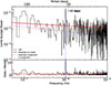 |
Fig. 2. LSP of the 0.3–2 keV light curve during phase 1b. The red solid curve represents the best-fit power-law + constant model. The blue vertical line marks the frequency of the QPO at approximately 1 × 10⁻⁶ Hz (∼12 days). The lower panel shows the data-to-model ratio as a function of frequency, where the QPO feature is clearly visible after subtracting the continuum modeled by the power-law + constant model. |
To estimate the QPO significance while properly accounting for the underlying noise, we fit the LSP using the following model,
 (1)
(1)
where N is the normalization factor, α is the power-law index, and C represents the combined contribution of Poisson noise and the aliasing level. To avoid bias, we excluded the 10 frequency bins surrounding the QPO frequency from the fit. The power-law component accounts for the red noise. We used the maximum likelihood estimation method to obtain the best-fit parameters (Vaughan 2010; Barret & Vaughan 2012; Lin et al. 2013). The best-fit normalization, power-law index, and constant were (1.5 ± 0.3) × 10−4, 0.3 ± 0.2, and 0.0031 ± 0.0004, respectively.
We note that uneven sampling may introduce systematic bias in the estimation of the power-law slope from the LSP (Uttley et al. 2002; Pasham et al. 2024b). To assess whether the current sampling might have influenced our estimate of the index, we conducted the following tests. We generated 100 000 simulated light curves using the method described by Timmer & König (1995), in which each light curve follows a power spectrum defined by the best-fitting power-law + constant model derived from the observed data. The time resolution of the simulated data was set to 100 seconds. To mitigate the effects of red-noise leakage (Uttley et al. 2002), the duration of each simulation was extended to ten times the observed baseline, which spans approximately 220 days. Each simulated light curve was then resampled to match the temporal sampling of the real observations and a LSP was computed for each case. These LSPs were subsequently fitted with a power-law + constant model. We analyzed the distribution of best-fitting indices from the 100 000 simulations. The resulting values have a median of 0.31 and a standard deviation of 0.03, closely matching the index obtained from the observed light curve. This result demonstrates that the spectral slope measured from our LSP analysis is a robust representation of the intrinsic variability power spectrum.
Following these results, we adopted a power-law + constant model to describe the underlying noise continuum. We then sought to evaluate the statistical significance of the QPO-like feature observed in the real data, which spans multiple frequency bins. To account for possible uncertainties in the PSD continuum, we therefore consider three noise continuum models (Pasham et al. 2024b):
-
Model A: best-fit power-law + constant model, with parameters (index, normalization) = (0.3, 1.5 × 10⁻⁴).
-
Model B: red-noise model using the best-fit index +1σ uncertainty, with (index, normalization) = (0.5, 1.2 × 10⁻⁵).
-
Model C: red-noise model with the best-fit normalization +1σ uncertainty, with (index, normalization) = (0.25, 1.8 × 10⁻⁴).
The significance of the signal is evaluated under all three models using the same procedure described in Appendix B, namely, a set of Monte Carlo simulations of time series.
With this rigorous simulation-based approach, which considers not only the best-fit model (model A) but also two conservative variants (models B and C), we obtained significance levels of 99.985%, 99.971%, and 99.937%, respectively (Fig. 3). Considering that we performed independent signal searches in both phase 1a and phase 1b, the global false alarm probabilities are doubled and the corresponding significance reduced accordingly. Assuming a normal distribution, these correspond to final global significance levels of 3.4σ, 3.3σ, and 3.2σ, respectively. It is worth mentioning that sampling-induced effects may also play a role in shaping the observed signal, as phase 1b includes a total of 118 individual observations; among these, approximately 26 fall close to the flux maximum. To assess this possibility, we performed Monte Carlo simulations adopting the best-fit continuum model (model A) as the underlying LSP shape, assuming that the intrinsic phase and the time of the first observation are random with respect to each other. We generated 10 000 synthetic light curves sampled at exactly the same time stamps as the real data and we found that the probability of obtaining ≥26 peak-hitting points is about 21%.
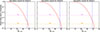 |
Fig. 3. Global false alarm probability of finding a multi-component peak in the simulated LSPs. Each of the three panels presents simulation results computed using the continuum models of model A, model B, and model C, respectively. The dashed, vertical blue line in each panel represent the observed ∑p, max, obs at 12 days. The violet and orange dashed horizontal lines mark the locations of 3σ and 4σ, respectively. |
4. Discussion
Having established that the QPO during phase 1b is statistically significant, we went on to set a constraint on the origin of the extreme X-ray variability. A series of studies have suggested that the event was triggered by an episodic accretion at the outer disk, likely resulting from the tidal disruption of a red giant star by the central black hole (Ricci et al. 2020, 2021; Cao et al. 2023). This event is believed to have swept away the pre-existing thin disk and corona upon reaching the innermost stable circular orbit (ISCO). Magnetic fields anchored to the disrupted star were advected inward by the post-TDE disk, powering strong outflows. As energy from the disk was largely channeled into these outflows, the disk itself was dimmed. Over time, as the accretion rate declined, the disk could no longer sustain significant magnetic advection, thereby decreasing the outflows. Eventually, a reformed corona emerged, corresponding to the phase 1b data in Fig. 1 (Cao et al. 2023).
Given that phase 1b marks the reformation of the corona and a return to a typical AGN-like state, it is of particular interest that a QPO signal emerges during this period. In the following, we discuss several potential models that may account for the QPO.
4.1. QPO potentially caused by line-of-sight neutral column density changes
The extreme event observed before and during phase-1a, interpreted as a TDE (Ricci et al. 2021; Cao et al. 2023), might have driven 1ES 1927+654 into a near- or super-Eddington accretion regime. Such high accretion rates are theoretically expected to launch powerful outflows of ionized gas. These outflows could intermittently intercept the observer’s line of sight, leading to variable absorption and modulations in the observed X-ray flux. To test this scenario, we extracted NICER spectra from intervals corresponding to high and low X-ray flux states during the QPO phase. Specifically, we selected five observations near the flux maxima (corresponding to obsIDs 1200190259, 1200190275, 2200190211, 2200190234, and 2200190245) and five near the minima (corresponding to obsIDs 1200190249, 1200190263, 1200190279, 2200190209, and 2200190217) within the QPO cycle. A spectral fitting using the XSPEC model tbabs*ztbabs*(zbb+zpower) yielded best-fit column densities for the ztbabs component that were all consistently low (NH ≤ 1021 cm−2), in agreement with the results of Ricci et al. (2021) and Masterson et al. (2022). These results suggest that the observed X-ray flux variations were not driven by changes in the line-of-sight neutral column density.
4.2. QPO possibly modulated by coronal oscillations
An X-ray spectral fitting of 1ES 1927+654 during phase-1b indicates that the 0.3–2 keV emission is primarily dominated by inverse Compton scattering from the corona (Ricci et al. 2020, 2021; Masterson et al. 2022). Theoretical studies have demonstrated that perturbations at the outer boundary of the corona can generate magnetoacoustic waves that propagate throughout the coronal region (Cabanac et al. 2010). These waves can modulate the Comptonization efficiency and induce oscillations on characteristic timescales of
 (2)
(2)
where cs is the sound speed in the plasma and rc represents the radial extent of the corona. Assuming a plasma temperature of T = 2 × 10⁸ K (Laha et al. 2025; Masterson et al. 2025) and a central black hole mass of MBH = 106 M⊙ (Li et al. 2022), the 10−6 z QPO observed during phase-1b implies a coronal radial extent of approximately rc ∼ 4500 Rs, where Rs = 2GM/c2 is the Schwarzschild radius. Such a large spatial scale far exceeds the typical coronal size inferred in AGNs, which is generally constrained to lie within a few tens of Rs. Although coronal oscillations are unlikely, we cannot rule out the possibility that fluctuations generated in the outer disk may propagate inward on thermal or viscous timescales and indirectly modulate the coronal emission, a possibility that would require further investigation beyond the scope of this work.
4.3. QPO possibly driven by accretion disk precession
An accretion disk formed around a SMBH after it disrupts a star is expected to be initially misaligned with respect to the equatorial plane of the black hole. This misalignment induces relativistic torques (i.e., the Lense-Thirring effect) on the disk, causing the disk to precess at early time; whereas at late times the disk aligns with the black hole and precession terminates (Stone & Loeb 2012; Franchini et al. 2016). Such a scenario is observationally supported by sources such as AT2020ocn and 3XMM J215022.4-055108 (Pasham et al. 2024b; Zhang et al. 2025), the former exhibited quasiperiodic modulations in both X-ray flux and blackbody temperature, with a period of 15 days persisting for approximately 130 days during the early phase of the TDE. While the oscillation period in 1ES 1927+654 is comparable, a key difference lies in the timing; the QPO in 1ES 1927+654 was detected more than 250 days after the TDE-related X-ray luminosity peak, by which time the TDE-related flux had already undergone a decline to its minimum value. In contrast, the periodic signal in AT2020ocn emerged shortly after the onset of X-ray emission, consistent with the timescale predicted by Lense–Thirring precession models. Moreover, during the oscillation phase in 1ES 1927+654, the X-ray spectrum was dominated by inverse Compton emission from a reformed corona, rather than thermal disk emission (Masterson et al. 2022). In addition, disk precession generally predict modulation amplitudes much smaller than the nearly two orders of magnitude variations we observe (Fig. 1, top panel; also see Śniegowska et al. 2023 and Pasham et al. 2024b). These properties strongly disfavor a Lense–Thirring effect origin for the 12 day QPO observed in 1ES 1927+654.
4.4. QPO originate from disk instability
In contrast, such large-amplitude luminosity variations are naturally expected from radiation pressure driven disk instabilities (Śniegowska et al. 2023; Pasham et al. 2024b). The inner region of a thin disk, where radiation pressure dominates, is thermally and viscously unstable (Shakura & Sunyaev 1976). This instability has been invoked to explain repeating X-ray burst phenomena, such as the “heartbeat” oscillations in X-ray binaries, CL AGNs, and QPEs (Wu et al. 2016; Pan et al. 2021, 2022; Kaur et al. 2023). The same physical mechanism may also be responsible for the QPO observed in our study. The timescale of the limit-cycle caused by these instabilities can be estimated by the range of the unstable region, Runstable, and the radial inflow velocity of local disk, VR,
 (3)
(3)
where RISCO is the radius of ISCO. As discussed in numerous studies (Lawrence 2018), the viscous timescale in a standard thin accretion disk around a SMBH is typically much longer than the observational history. However, this discrepancy can be resolved by incorporating a large-scale magnetic field into the accretion system (Cao & Spruit 2013; Feng et al. 2021). Magnetically driven outflows can simultaneously reduce the size of the unstable region and increase the radial inflow velocity by extracting energy and angular momentum from the disk. Following the model of Pan et al. (2021), the outer boundary of the unstable zone can be determined by the accretion rate and the magnetic field parameter, assuming a fixed viscosity parameter. In this work, we develop a toy model (see Appendix C) and provide an analytical equation for the outer boundary of the unstable region,
![Mathematical equation: $$ \begin{aligned} R_{\rm unstable} = 1.875\times 10^{6}\frac{\alpha m\dot{m}(1+\beta _{1})}{C_{0}\pi \beta _{1}(1-\beta _{2})}\,[\mathrm {cm}], \end{aligned} $$](/articles/aa/full_html/2025/12/aa56066-25/aa56066-25-eq4.gif) (4)
(4)
where α is the viscous parameter and we adopt α = 0.1 in this work, m (=M/M⊙) is the black hole mass, and ṁ (= Ṁ/ṀEdd, ṀEdd = 1.5 × 10¹⁸m [g s−1]) is the accretion rate. The parameters β1, β2, and C0, which characterize the magnetic field strength, the ratio of gas pressure to the sum of gas and radiation pressures, and the magnetic field configuration, respectively, are defined in the Appendix C. In addition, we provide a simple equation for the local radial velocity of the accretion disk from our toy model,
![Mathematical equation: $$ \begin{aligned} V_{\rm R} = 9.084\times 10^{3}\left[\frac{\beta _{1}}{2C_{0}^{2}T(1+\beta _{1})}-\frac{3.125\alpha \dot{m}}{\pi C_{0}^3Tr}\right]^{-1/2}\,[\mathrm {cm\,s}^{-1}], \end{aligned} $$](/articles/aa/full_html/2025/12/aa56066-25/aa56066-25-eq5.gif) (5)
(5)
where r = R/Rs, and T, the temperature of the middle plane, can be written as
![Mathematical equation: $$ \begin{aligned} T = 1.601\times 10^{8}\left[\frac{\alpha \dot{m}^{2}}{C_{0}^2\pi ^{2}r^{7/2}m}\right]^{1/4}\,[\mathrm K]. \end{aligned} $$](/articles/aa/full_html/2025/12/aa56066-25/aa56066-25-eq6.gif) (6)
(6)
The local instability criterion is β2 < 0.4 if we adopt the αP prescription for viscosity. Therefore, we can obtain the repeating timescale for the disk instability when we provide a set of m, ṁ, and β1. We set the black hole mass of 1ES 1927+654 as m = 106 and our analysis yields the repeating timescale as a function of both the accretion rate and magnetic field parameter, as shown in Fig. 4.
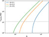 |
Fig. 4. Timescale of repeating disk instabilities, with curves representing different accretion rates: ṁ = 0.5 (green), 0.3 (orange), and 0.1 (blue). The dashed gray line marks the characteristic QPO timescale for comparison. |
According to the model proposed by Cao et al. (2023), the TDE in this source may have disrupted a red giant star. In this scenario, the red giant’s magnetic field was dragged into the accretion disk following the disruption, successfully explaining both the disappearance and subsequent reappearance of the corona. Adopting the same physical scenario, we suggest that when the accretion rate and magnetic field strength in 1ES 1927+654 reach appropriate values, radiation-pressure instability can trigger recurring outbursts in the inner accretion disk. This mechanism provides a plausible explanation for the observed large-amplitude X-ray flux variations and the QPO during phase 1b.
A fundamental requirement for the radiation pressure instability mechanism in our model is the maintenance of sub-Eddington accretion rates (ṁ < 1) in the inner disk region. However, spectral energy distribution (SED) analysis reveals that the source exhibits super-Eddington accretion (ṁ > 1, Li et al. 2024) during its phase-1 stage. This apparent inconsistency can be reconciled through the combined effects of radiation-driven and magnetically driven outflows from the accretion disk. Under super-Eddington conditions, the vertical radiation force may exceed local gravity, launching outflows that remove sufficient mass to maintain the inner disk’s accretion rate near the Eddington limit (Feng et al. 2019; Cao & Gu 2022). Additionally, magnetically driven outflows could further reduce the global accretion rate (Li & Cao 2019). Consequently, while the outer disk might have super-Eddington accretion, the innermost region can remain sub-Eddington, enabling radiation pressure instability to operate and produce the observed QPO.
In accretion theory, the disk remains stable in the low accretion rate regime, where radiation pressure is negligible, as well as in the high accretion rate regime, where advective cooling via photon trapping effect becomes dominant. However, at intermediate accretion rates. where radiation pressure and radiative cooling prevail, the disk is expected to become thermally and viscously unstable, potentially giving rise to global limit-cycle oscillations between high (advection-dominated) and low (gas-pressure-dominated) accretion states. Despite these theoretical expectations, observations show that most AGNs appear to be in stable accretion states, suggesting that additional physical mechanisms may act to suppress or moderate these instabilities, as illustrated by the extreme event in 1ES 1927+654 (possibly a TDE).
5. Conclusion
1ES 1927+654 was initially identified as a type 2 Seyfert galaxy. Multi-wavelength observations revealed that an extreme event had occurred in the vicinity of the central SMBH, possibly a TDE, followed by a spectroscopic CL phenomenon. High-cadence X-ray monitoring showed that the inner disk-corona underwent a process of destruction and subsequent reformation. During the reformation of the inner disk-corona, we detected a significant QPO with a period of ∼12 days in its long-term X-ray light curve, and the coherent signal, with a very high quality factor of ∼58, lasts for approximately 220 days. Models involving line-of-sight neutral column density variations, coronal oscillations, and accretion disk precession cannot fully account for all the observed properties of the QPO. We interpret this periodicity as a signature of radiation-pressure instability in the accretion disk, which occurs when the accretion rate and magnetic field strength reach appropriate values, a theory that has already been effectively applied to QPEs (Pan et al. 2021, 2022). Although radiation-pressure instability in the accretion disk has long been predicted by accretion theory, it has rarely been observed in AGNs. As a result, 1ES 1927+654 could represent one of the first significant cases in which the post-TDE evolution of an AGN’s accretion disk and corona can be directly investigated through observational data.
Acknowledgments
This research made use of the HEASARC online data archive services, supported by NASA/GSFC, and is based on observations obtained with NICER, a mission of NASA’s Explorers Program designed to study the extreme physics of neutron stars and black holes. This work is supported by the Postdoctoral Fellowship Program of CPSF (Grant NO. GZC20232699 and GZC20232696), National Natural Science Foundation of China (Grant NO. 12433005, 12333004, 12192220 and 12192221) and National Key Research and Development Program of China (Grant NO. 2022SKA0130102).
References
- Arcodia, R., Merloni, A., Nandra, K., et al. 2021, Nature, 592, 704 [NASA ADS] [CrossRef] [Google Scholar]
- Barret, D., & Vaughan, S. 2012, ApJ, 746, 131 [NASA ADS] [CrossRef] [Google Scholar]
- Blanchard, P. K., Nicholl, M., Berger, E., et al. 2017, ApJ, 843, 106 [Google Scholar]
- Bykov, S. D., Gilfanov, M. R., Sunyaev, R. A., et al. 2025, MNRAS, 540, 30 [Google Scholar]
- Cabanac, C., Henri, G., Petrucci, P.-O., et al. 2010, MNRAS, 404, 738 [NASA ADS] [CrossRef] [Google Scholar]
- Cao, X., & Gu, W.-M. 2022, ApJ, 936, 141 [Google Scholar]
- Cao, X., & Spruit, H. C. 2013, ApJ, 765, 149 [NASA ADS] [CrossRef] [Google Scholar]
- Cao, X., You, B., & Wei, X. 2023, MNRAS, 526, 2331 [NASA ADS] [CrossRef] [Google Scholar]
- Chakraborty, J., Kara, E., Masterson, M., et al. 2021, ApJ, 921, L40 [NASA ADS] [CrossRef] [Google Scholar]
- Chan, C.-H., Piran, T., Krolik, J. H., et al. 2019, ApJ, 881, 113 [NASA ADS] [CrossRef] [Google Scholar]
- Chan, C.-H., Piran, T., & Krolik, J. H. 2020, ApJ, 903, 17 [CrossRef] [Google Scholar]
- Feng, J., Cao, X., Gu, W.-M., et al. 2019, ApJ, 885, 93 [Google Scholar]
- Feng, J., Cao, X., Li, J.-W., et al. 2021, ApJ, 916, 61 [NASA ADS] [CrossRef] [Google Scholar]
- Franchini, A., Lodato, G., & Facchini, S. 2016, MNRAS, 455, 1946 [NASA ADS] [CrossRef] [Google Scholar]
- Franchini, A., Bonetti, M., Lupi, A., et al. 2023, A&A, 675, A100 [NASA ADS] [CrossRef] [EDP Sciences] [Google Scholar]
- Gallo, L. C., MacMackin, C., Vasudevan, R., et al. 2013, MNRAS, 433, 421 [Google Scholar]
- Gendreau, K. C., Arzoumanian, Z., & Okajima, T. 2012, Proc. SPIE, 8443, 844313 [NASA ADS] [CrossRef] [Google Scholar]
- Ghosh, R., Laha, S., Meyer, E., et al. 2023, ApJ, 955, 3 [Google Scholar]
- Gilbert, O., Ruan, J. J., Eracleous, M., et al. 2024, ApJ, submitted [arXiv:2409.10486] [Google Scholar]
- Giustini, M., Miniutti, G., & Saxton, R. D. 2020, A&A, 636, L2 [NASA ADS] [CrossRef] [EDP Sciences] [Google Scholar]
- González-Martín, O., & Vaughan, S. 2012, A&A, 544, A80 [NASA ADS] [CrossRef] [EDP Sciences] [Google Scholar]
- Horne, J. H., & Baliunas, S. L. 1986, ApJ, 302, 757 [Google Scholar]
- Jana, A., Ricci, C., Temple, M. J., et al. 2025, A&A, 693, A35 [NASA ADS] [CrossRef] [EDP Sciences] [Google Scholar]
- Jiang, N., & Pan, Z. 2025, ApJ, 983, L18 [Google Scholar]
- Kang, J.-L., Done, C., Hagen, S., et al. 2025, MNRAS, 538, 121 [Google Scholar]
- Karas, V., & Šubr, L. 2007, A&A, 470, 11 [NASA ADS] [CrossRef] [EDP Sciences] [Google Scholar]
- Kaur, K., Stone, N. C., & Gilbaum, S. 2023, MNRAS, 524, 1269 [NASA ADS] [CrossRef] [Google Scholar]
- Kennedy, G. F., Meiron, Y., Shukirgaliyev, B., et al. 2016, MNRAS, 460, 240 [NASA ADS] [CrossRef] [Google Scholar]
- Laha, S., Meyer, E., Roychowdhury, A., et al. 2022, ApJ, 931, 5 [NASA ADS] [CrossRef] [Google Scholar]
- Laha, S., Meyer, E. T., Sadaula, D. R., et al. 2025, ApJ, 981, 125 [Google Scholar]
- LaMassa, S. M., Cales, S., Moran, E. C., et al. 2015, ApJ, 800, 144 [NASA ADS] [CrossRef] [Google Scholar]
- Lawrence, A. 2018, Nat. Astron., 2, 102 [NASA ADS] [CrossRef] [Google Scholar]
- Li, J., & Cao, X. 2019, ApJ, 872, 149 [NASA ADS] [CrossRef] [Google Scholar]
- Li, R., Ho, L. C., Ricci, C., et al. 2022, ApJ, 933, 70 [NASA ADS] [CrossRef] [Google Scholar]
- Li, R., Ricci, C., Ho, L. C., et al. 2024, ApJ, 975, 140 [NASA ADS] [CrossRef] [Google Scholar]
- Lin, D., Irwin, J. A., Godet, O., et al. 2013, ApJ, 776, L10 [NASA ADS] [CrossRef] [Google Scholar]
- Linial, I., & Metzger, B. D. 2023, ApJ, 957, 34 [NASA ADS] [CrossRef] [Google Scholar]
- MacLeod, C. L., Ross, N. P., Lawrence, A., et al. 2016, MNRAS, 457, 389 [Google Scholar]
- Markowitz, A., Edelson, R., Vaughan, S., et al. 2003, ApJ, 593, 96 [NASA ADS] [CrossRef] [Google Scholar]
- Masterson, M., Kara, E., Ricci, C., et al. 2022, ApJ, 934, 35 [NASA ADS] [CrossRef] [Google Scholar]
- Masterson, M., Kara, E., Panagiotou, C., et al. 2025, Nature, 638, 370 [Google Scholar]
- Meyer, E. T., Laha, S., Shuvo, O. I., et al. 2025, ApJ, 979, L2 [Google Scholar]
- Miniutti, G., Saxton, R. D., Giustini, M., et al. 2019, Nature, 573, 381 [Google Scholar]
- Nicholl, M., Pasham, D. R., Mummery, A., et al. 2024, Nature, 634, 804 [CrossRef] [Google Scholar]
- Pan, X., Li, S.-L., & Cao, X. 2021, ApJ, 910, 97 [NASA ADS] [CrossRef] [Google Scholar]
- Pan, X., Li, S.-L., Cao, X., et al. 2022, ApJ, 928, L18 [NASA ADS] [CrossRef] [Google Scholar]
- Pan, X., Li, S.-L., & Cao, X. 2023, ApJ, 952, 32 [CrossRef] [Google Scholar]
- Pasham, D. R., Ho, W. C. G., Alston, W., et al. 2021, Nat. Astron., 6, 249 [NASA ADS] [CrossRef] [Google Scholar]
- Pasham, D. R., Lucchini, M., Laskar, T., et al. 2023, Nat. Astron., 7, 88 [Google Scholar]
- Pasham, D. R., Tombesi, F., Suková, P., et al. 2024a, Sci. Adv., 10, eadj8898 [Google Scholar]
- Pasham, D. R., Zajaček, M., Nixon, C. J., et al. 2024b, Nature, 630, 325 [NASA ADS] [CrossRef] [Google Scholar]
- Raj, A., & Nixon, C. J. 2021, ApJ, 909, 82 [NASA ADS] [CrossRef] [Google Scholar]
- Remillard, R. A., Loewenstein, M., Steiner, J. F., et al. 2022, AJ, 163, 130 [NASA ADS] [CrossRef] [Google Scholar]
- Ricci, C., Kara, E., Loewenstein, M., et al. 2020, ApJ, 898, L1 [Google Scholar]
- Ricci, C., Loewenstein, M., Kara, E., et al. 2021, ApJS, 255, 7 [NASA ADS] [CrossRef] [Google Scholar]
- Scargle, J. D. 1982, ApJ, 263, 835 [Google Scholar]
- Scepi, N., Begelman, M. C., & Dexter, J. 2021, MNRAS, 502, L50 [NASA ADS] [CrossRef] [Google Scholar]
- Shakura, N. I., & Sunyaev, R. A. 1976, MNRAS, 175, 613 [NASA ADS] [CrossRef] [Google Scholar]
- Shappee, B. J., Prieto, J. L., Grupe, D., et al. 2014, ApJ, 788, 48 [Google Scholar]
- Sheng, Z., Wang, T., Jiang, N., et al. 2017, ApJ, 846, L7 [NASA ADS] [CrossRef] [Google Scholar]
- Sheng, Z., Wang, T., Ferland, G., et al. 2021, ApJ, 920, L25 [NASA ADS] [CrossRef] [Google Scholar]
- Shu, X. W., Wang, S. S., Dou, L. M., et al. 2018, ApJ, 857, L16 [NASA ADS] [CrossRef] [Google Scholar]
- Śniegowska, M., Grzȩdzielski, M., Czerny, B., et al. 2023, A&A, 672, A19 [NASA ADS] [CrossRef] [EDP Sciences] [Google Scholar]
- Stone, N., & Loeb, A. 2012, Phys. Rev. Lett., 108, 061302 [NASA ADS] [CrossRef] [Google Scholar]
- Timmer, J., & König, M. 1995, A&A, 300, 707 [Google Scholar]
- Trakhtenbrot, B., Arcavi, I., MacLeod, C. L., et al. 2019, ApJ, 883, 94 [Google Scholar]
- Uttley, P., McHardy, I. M., & Papadakis, I. E. 2002, MNRAS, 332, 231 [Google Scholar]
- van der Klis, M. 1989, Timing Neutron Stars, 262, 27 [NASA ADS] [CrossRef] [Google Scholar]
- Vaughan, S. 2010, MNRAS, 402, 307 [NASA ADS] [CrossRef] [Google Scholar]
- Wevers, T., Pasham, D. R., Jalan, P., et al. 2022, A&A, 659, L2 [NASA ADS] [CrossRef] [EDP Sciences] [Google Scholar]
- Wevers, T., French, K. D., Zabludoff, A. I., et al. 2024, ApJ, 970, L23 [NASA ADS] [CrossRef] [Google Scholar]
- Wu, Q., Czerny, B., Grzedzielski, M., et al. 2016, ApJ, 833, 79 [NASA ADS] [CrossRef] [Google Scholar]
- Xian, J., Zhang, F., Dou, L., et al. 2021, ApJ, 921, L32 [NASA ADS] [CrossRef] [Google Scholar]
- Zhang, W. J., Shu, X. W., Sheng, Z. F., et al. 2022a, A&A, 660, A119 [NASA ADS] [CrossRef] [EDP Sciences] [Google Scholar]
- Zhang, W., Shu, X., Chen, J.-H., et al. 2022b, Res. Astron. Astrophys., 22, 125016 [CrossRef] [Google Scholar]
- Zhang, W., Shu, X., Sun, L., et al. 2025, Nat. Astron., 9, 702 [Google Scholar]
- Zhou, C., Huang, L., Guo, K., et al. 2024, Phys. Rev. D, 109, 103031 [NASA ADS] [CrossRef] [Google Scholar]
Appendix A: Light-curve sampling interval distribution
To test whether the observed QPO feature could be affected by aliasing introduced by irregular sampling, we examined the distribution of time intervals between successive observations. Aliasing effects are expected when the effective sampling approaches the Nyquist limit, potentially producing artificial excess power just below this frequency (Uttley et al. 2002; van der Klis 1989). For a more detailed check, we divided phase 1b into two halves at the midpoint (2019-04-14) and examined both the sampling histograms (Fig. A.1) and LSP (Fig. A.2). We note that intervals of about ∼6 days are present only in the first half of phase 1b, and do not occur in the second half. Despite this difference in sampling, both halves exhibit a QPO signal at ∼12 days. Despite this difference in sampling, both halves exhibit a QPO signal at ∼12 days, supporting the interpretation that the detected feature is not simply an aliasing artifact of the sampling pattern.
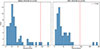 |
Fig. A.1. Histogram of sampling intervals distributions of phase 1b (left: first half; right: second half, split at 2019-04-14). The ∼6 day (144 hr) intervals occur only in the first half. |
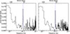 |
Fig. A.2. LSP of phase 1b, divided into two halves at 2019-04-14 (left: first half, right: second half). Both segments exhibit a QPO signal at ∼12 days. |
Appendix B: Monte Carlo simulations of time series
-
We simulated 100,000 LSPs using the algorithm from Timmer & König (1995), matching the temporal sampling of the observed light curve, and computed their median spectrum (LSPmedian).
-
Each simulated LSP was normalized by dividing its power at each frequency by the corresponding value from LSPmedian. This yielded a set of 100,000 normalized LSPs dominated by white noise, with a mean power of 1.
-
In each normalized LSP, we searched for QPO-like features across all frequencies by fitting a constant + Lorentzian model. The Lorentzian centroid was allowed to vary across 10−7–10−5 Hz, and the width was treated as a free parameter but constrained such that the resulting quality factor remained within Q = 58 ± 11 (90% confidence level; i.e., 47–69).
-
For each simulated LSP, we summed the powers within the width of the best-fit Lorentzian at every frequency, denoting this value as ∑p, and recorded the maximum value across all frequencies as ∑p,max. Repeating this for all simulated LSPs resulted in a distribution of 100,000 ∑p,max values.
-
We then constructed a cumulative distribution function (CDF) of all the ∑p,max values (Fig. 3).
-
Finally, we applied the same steps (1–3) to the observed LSP to obtain ∑p,max,obs, which we overlaid on the simulated CDF. In all cases, the peak signal occurred near 12 days.
Appendix C: Thin disk model with large-scale magnetic field
Here we present the key assumptions and basic equations of our accretion disk instability model with large-scale magnetic fields, as introduced in Section 4.4. Since our goal is to derive a simple analytical expression for the instability recurrence timescale, we adopt a non-spinning black hole and apply the Newtonian potential approximation. Following the magnetic field configuration of Pan et al. (2021), we set Bϕ = 0.15Bp and adopt an inclination angle of 60 degrees for our analysis. Given that the outflow rate remains negligible under these conditions, we ignore its contribution to the accretion rate.
In regimes with non-weak magnetic fields where magnetic torque dominates angular momentum transport (Cao & Spruit 2013), we neglect the viscous term in the angular momentum equation,
 (C.1)
(C.1)
where Tm (=BzBϕR/2π) is the magnetic torque exerted on the accretion flow, and lk ( ) is the specific angular momentum.
For thin disks, the energy equation can be written as
 (C.2)
(C.2)
where ν (=αcsH, with  ) is the viscosity coefficient, and τ (=κesΣ/2) is the optical depth.
The equation of state in our model is
 (C.3)
(C.3)
where β1 = (Pgas + Prad)/(B2/8π), Pgas = ΣkBT/mHH, and Prad = aT4/3 (with a being the radiation constant).
From vertical hydrostatic equilibrium, the scale height is given by H = cs/Ωk. Meanwhile, the adopted magnetic field configuration yields a magnetic torque term of Tm = C0PR, where C0 = 0.508/(1 + β1) in our model. Therefore, we can derive an analytical expression for the temperature T (Equation 6) by solving Equation C.2, and the gas pressure ratio β2 = Pgas/(Pgas + Prad) can be obtained from Equations C.2 and C.3:
 (C.4)
(C.4)
Once the instability criterion is established, the outer boundary of the unstable region can be determined by solving this equation, as presented in the main text (Equation 4). By combining Equation C.1 with the mass conservation relation Ṁ = 2 π RΣ VR, we derive the radial velocity expression given in Equation 5 of the main text.
We note that Equation C.4 yields negative values in the inner disk region. This arises from our key assumption that magnetic torque dominates angular momentum transport, which is only valid in the middle and outer disk regions, where β2 does not approach zero. Nevertheless, this limitation has small impact on determining the extent of the unstable zone, since the αP prescription places the outer boundary of the instability at β2 = 0.4.
All Figures
|
Fig. 1. Top panel: 0.3–10 keV NICER X-ray light curve for 1ES 1927+654 since May 2018 (blue). Following the methodology of Masterson et al. (2022), we divided the long-term X-ray light curve of 1ES 1927+654 into distinct phases. Phase 1 is characterized by a super-Eddington state with rapid fluctuations in both X-ray luminosity and spectral parameters. Phase 2 maintains a stable super-Eddington luminosity near its peak. Phase 3 exhibits a gradual decline in X-ray luminosity and spectral parameters, returning to levels comparable to those observed prior to the outburst. Phase 1 is divided into two equal segments and phase 1b is between the two vertical dashed red lines in phase 1. Bottom panel: Observation data in phase 1b plotted as black points after binning all observations within three-day intervals for visual clarity. To enhance the visibility of the periodic signal, we applied the logarithmic function f(x) = A ⋅ log(Bx + C)+D and removed the long-term trend, connecting the data and model points with a smoothed curve. Note: this approach is intended solely for visual illustration of periodicity. Dashed gray vertical lines denote a period of 11.6 days. |
| In the text | |
|
Fig. 2. LSP of the 0.3–2 keV light curve during phase 1b. The red solid curve represents the best-fit power-law + constant model. The blue vertical line marks the frequency of the QPO at approximately 1 × 10⁻⁶ Hz (∼12 days). The lower panel shows the data-to-model ratio as a function of frequency, where the QPO feature is clearly visible after subtracting the continuum modeled by the power-law + constant model. |
| In the text | |
|
Fig. 3. Global false alarm probability of finding a multi-component peak in the simulated LSPs. Each of the three panels presents simulation results computed using the continuum models of model A, model B, and model C, respectively. The dashed, vertical blue line in each panel represent the observed ∑p, max, obs at 12 days. The violet and orange dashed horizontal lines mark the locations of 3σ and 4σ, respectively. |
| In the text | |
|
Fig. 4. Timescale of repeating disk instabilities, with curves representing different accretion rates: ṁ = 0.5 (green), 0.3 (orange), and 0.1 (blue). The dashed gray line marks the characteristic QPO timescale for comparison. |
| In the text | |
|
Fig. A.1. Histogram of sampling intervals distributions of phase 1b (left: first half; right: second half, split at 2019-04-14). The ∼6 day (144 hr) intervals occur only in the first half. |
| In the text | |
|
Fig. A.2. LSP of phase 1b, divided into two halves at 2019-04-14 (left: first half, right: second half). Both segments exhibit a QPO signal at ∼12 days. |
| In the text | |
Current usage metrics show cumulative count of Article Views (full-text article views including HTML views, PDF and ePub downloads, according to the available data) and Abstracts Views on Vision4Press platform.
Data correspond to usage on the plateform after 2015. The current usage metrics is available 48-96 hours after online publication and is updated daily on week days.
Initial download of the metrics may take a while.