| Issue |
A&A
Volume 704, December 2025
|
|
|---|---|---|
| Article Number | A192 | |
| Number of page(s) | 8 | |
| Section | Extragalactic astronomy | |
| DOI | https://doi.org/10.1051/0004-6361/202556215 | |
| Published online | 09 December 2025 | |
A timescale-resolved analysis of the breathing effect in quasar broad-line regions
1
Department of Astronomy, University of Science and Technology of China, Hefei, Anhui 230026, People’s Republic of China
2
School of Astronomy and Space Science, University of Science and Technology of China, Hefei 230026, People’s Republic of China
3
Department of Physics and Astronomy, University of California, Riverside, 900 University Ave, Riverside, CA 92521, USA
4
College of Physics, Guizhou University, Guiyang, Guizhou 550025, People’s Republic of China
★ Corresponding authors: This email address is being protected from spambots. You need JavaScript enabled to view it.
; This email address is being protected from spambots. You need JavaScript enabled to view it.
Received:
2
July
2025
Accepted:
9
November
2025
Abstract
Context. The single-epoch virial method is a fundamental tool for estimating supermassive black hole (SMBH) masses in large samples of active galactic nuclei (AGNs) and has been extensively employed in studies of SMBH–galaxy coevolution across cosmic time. However, since this method is calibrated using reverberation-mapped AGNs, its validity across the entire AGN population remains uncertain.
Aims. We aim to examine the breathing effect–the variability of emission line widths with continuum luminosity–beyond reverberation-mapped AGNs, to assess the validity and estimate potential systematic uncertainties of single-epoch virial black hole mass estimates.
Methods. We constructed an unprecedentedly large multi-epoch spectroscopic dataset of quasars from Sloan Digital Sky Survey data release 16 (SDSS DR16), focusing on four key broad emission lines (Hα, Hβ, Mg II, and C IV). We assessed how breathing behavior evolves with the rest-frame time interval between observations.
Results. We detect no significant breathing signal in Hα, Hβ, or Mg II at any observed timescale. In contrast, C IV exhibits a statistically significant anti-breathing trend, most prominent at intermediate timescales. Notably, for Hβ, which has shown breathing in previous reverberation-mapped samples, we recover the effect only in the small subset of quasars with clearly detected broad-line region (BLR) lags and only during the epochs when such lags are measurable–suggesting that both the lag and breathing signals are intermittent, possibly due to a weak correlation between optical and ionizing continua. These results highlight the complex, variable, and timescale-dependent nature of line profile variability and underscore its implications for single-epoch black hole mass estimates.
Key words: galaxies: active / quasars: supermassive black holes
© The Authors 2025
 Open Access article, published by EDP Sciences, under the terms of the Creative Commons Attribution License (https://creativecommons.org/licenses/by/4.0), which permits unrestricted use, distribution, and reproduction in any medium, provided the original work is properly cited.
This article is published in open access under the Subscribe to Open model. This email address is being protected from spambots. You need JavaScript enabled to view it. to support open access publication.
1. Introduction
Broad emission lines are prominent features in the ultraviolet and optical spectra of active galactic nuclei (AGNs) and quasars. These lines serve as powerful diagnostics of the gas dynamics in the broad-line region (BLR), which lies within the gravitational potential of the central supermassive black hole (SMBH). As such, they offer a unique method for estimating SMBH masses (e.g., Woltjer 1959; Peterson & Wandel 2000; Peterson et al. 2004; Gaskell 2009). Assuming the BLR gas is virialized, the black hole mass can be estimated using the relation:
 (1)
(1)
where f is the dimensionless projection (or virial) factor accounting for the geometry and kinematics of the BLR, G is the gravitational constant, ΔV is the velocity dispersion of the BLR clouds (typically inferred from the Doppler broadening of the emission lines), and RBLR is the characteristic radius of the BLR.
With extensive monitoring campaigns over the past decades, empirical global relations between the BLR size and AGN luminosity (RBLR ∝ Lβ) have been established. These so-called RBLR–L relations hold for both low-ionization lines, such as Mg II (β ≃ 0.7; Shen et al. 2016; Homayouni et al. 2020) and Hβ (β ≃ 0.5; Kaspi et al. 2005; Bentz et al. 2009, 2013), as well as for high-ionization lines such as C IV (β ≃ 0.5; Lira et al. 2018; Kaspi et al. 2021). The relatively tight intrinsic scatter of these relations suggests that the BLR radius can be inferred from a single-epoch measurement, thus providing a practical alternative to reverberation mapping for estimating black hole masses. This single-epoch virial method has become a fundamental tool for estimating black hole masses in large samples of AGNs and has been widely employed in studies exploring the coevolution of SMBHs and their host galaxies.
Examining the variability of emission line widths with continuum or line luminosity–commonly referred to as the “breathing effect” – in AGNs with multi-epoch spectroscopic observations is a crucial approach for assessing the validity and estimating potential systematic uncertainties of single-epoch virial black hole mass estimates. However, the literature reports conflicting results regarding the breathing behavior.
In nearby Seyfert galaxies, reverberation mapping campaigns have shown that the Hβ line width tends to decrease as luminosity increases (e.g., Park et al. 2012; Barth et al. 2015). Combined with the finding that the Hβ lag scales with the mean continuum luminosity (e.g., Peterson et al. 2002), these results support a scenario in which the Balmer line-emitting region expands in response to enhanced ionizing radiation, consistent with photoionization model predictions (e.g., Korista & Goad 2004). Similar breathing behavior in Hβ has also been reported for large samples of quasars on average (Shen 2013; Wang et al. 2020).
Nevertheless, other studies have reported a lack of breathing in either Hβ or Hα in quasars (e.g., Guo & Gu 2014; Ren et al. 2024). Notably, while the Sloan Digital Sky Survey Reverberation Mapping (SDSS-RM, Shen et al. 2015) sample analyzed by Wang et al. (2020) shows a clear average breathing trend in Hβ, many individual quasars within the sample exhibit either no breathing or even anti-breathing (i.e., line width increasing with luminosity). Moreover, their study reported no significant average breathing in Hα, in contrast to the behavior seen in Hβ.
The picture becomes more complex when considering other emission lines. For Mg II, no or only weak breathing has been observed in quasars, including those with extreme variability (e.g., Shen 2013; Homan et al. 2020; Yang et al. 2020; Wang et al. 2020; Ren et al. 2024). In contrast, C IV commonly exhibits anti-breathing behavior in quasars (e.g., Richards et al. 2002, 2011; Wilhite et al. 2006; Shen et al. 2008), likely reflecting the influence of non-virial kinematics such as outflows or inflows in the emitting region. However, a lack of breathing in C IV has also been reported (Ren et al. 2024).
Taken together, these results highlight the diversity and complexity of breathing behaviors across different emission lines and AGN populations. The observed variability patterns–ranging from normal breathing to anti-breathing and non-detections–not only reflect differences in the physical and kinematic conditions of the line-emitting regions but also suggest that the underlying mechanisms driving line width variability may differ across sources and lines. A more comprehensive understanding of breathing behaviors is thus essential for refining these mass estimates and for improving their applicability across cosmic time and AGN types.
Recently, Ren et al. (2024) reported the absence of the breathing effect in Hβ, Mg II, and C IV for samples of extremely variable quasars, in contrast to previous studies of normal quasars. Since their data probe variability over much longer timescales (∼3000 days in the observed frame), they speculated that the breathing effect, if present, may weaken or even disappear on such long timescales. This raises an intriguing question of whether the breathing effect of different broad emission lines in regular quasars depends on the timescale of variability.
In principle, the response of the broad line width to continuum variations is expected to be timescale dependent. On timescales comparable to the broad-line lag, any intrinsic breathing signal would be smeared out or significantly suppressed due to the finite light-travel time across the BLR. Notably, correcting for this time lag is unfeasible for most studies, as it requires dense reverberation mapping data and reliable lag measurements (e.g., Wang et al. 2020).
At slightly longer timescales, the impact of the BLR lag may diminish, potentially allowing the intrinsic breathing trend to emerge more clearly. On much longer timescales, however, additional physical processes, such as structural changes in the BLR or turbulence within the accretion disk (Kang et al. 2021), may begin to dominate, possibly altering or masking the breathing behavior.
In this work, we utilized an unprecedentedly large sample of quasars with multi-epoch spectroscopic observations from Sloan Digital Sky Survey data release 16 (SDSS DR16) to systematically investigate the breathing effect in different broad emission lines. In particular, we present the first systematic study of the timescale dependence of quasar breathing by analyzing how the line width–luminosity correlation evolves across a wide range of temporal baselines.
The structure of this paper is as follows. In Sect. 2, we describe the dataset and the spectral decomposition techniques employed to measure the properties of the broad emission lines. In Sect. 3.1, we examine the overall breathing effects for four broad emission lines in our sample. In Sect. 3.2, we introduce a novel method to divide the sample according to different time baselines and assess how the observed breathing behavior varies with the timescale of variability. In Sect. 4, we discuss our results and the implications of our findings. We summarize our main findings in Sect. 5. Throughout this paper, we adopt a flat ΛCDM cosmology with ΩΛ = 0.7, Ωm = 0.3, and H0 = 70 km s−1 Mpc−1.
2. Data and reduction
2.1. Data
To construct our sample, we required quasars to have at least two spectroscopic observations in order to enable variability studies. Starting from the full catalog of 750 414 quasars in SDSS DR16 (DR16Q, Lyke et al. 2020), we performed a cross-match with the spectroscopic database using a 2″ search radius around each quasar’s coordinates. To ensure data consistency, we imposed additional criteria on the retrieved spectra: the relative difference between the pipeline redshifts of the two epochs must be less than 0.01 (|Δz|/(z0 + 1) < 0.01, where z0 is the primary redshift), removing irrelevant foreground and/or background galaxies.
2.2. Spectral measurement
We fit the retrieved spectra using the PYQSOFIT code (Guo et al. 2018), following the methodology described in Ren et al. (2024). The continuum was modeled as a powerlaw (fλ ∝ λα) combined with a broadened Fe II emission template, fit over a set of carefully selected line-free continuum windows. After subtracting the best-fit continuum and Fe II emission, we modeled the residual broad and narrow emission lines using multiple Gaussian components to capture their complex profiles. Narrow Gaussian lines were constrained to have FWHM (full width at half maximum) < 1200 km s−1, while broad Gaussian lines were required to have FWHM > 1200 km s−1.
The Hα and Hβ lines were each modeled with one narrow Gaussian and three broad Gaussians to fully represent their profiles. Each line in the [O III] λλ4959, 5007 doublet was modeled with one narrow (core) Gaussian and one broad (wing) Gaussian. The [N II] λλ6548, 6583 and [S II] λλ6716, 6731 doublets were each modeled with one narrow Gaussian per line. The Mg II and the C IV1 lines were each fitted with one narrow and two broad Gaussians. To minimize parameter degeneracies and ensure physical consistency, the widths and velocity offsets of the narrow Hβ and [O III] core components were tied together. Similarly, those of the narrow Hα, [N II] and [S II] components were linked. The flux ratios of the three line doublets ([O III], [N II] and [S II]) were left as free parameters, and we verified that the fitted ratios remained within physically reasonable ranges.
We estimated the statistical uncertainties of our measured parameters using a Monte Carlo approach. Specifically, we generated 200 mock spectra by adding Gaussian noise to the original spectrum, with the noise level determined by the flux errors provided in the pipeline. Each mock spectrum was then fit using the same procedures as the original data, and the scatter in the resulting parameters was used to quantify their uncertainties.
2.3. The final samples
After excluding unphysical fits and applying signal-to-noise ratio (S/N) thresholds (requiring S/N > 3 for the continuum and S/N > 3 for the emission lines), we identified four subsets of quasars with multiple SDSS spectroscopic observations and successful spectral fitting. This yielded 1945 quasars with 6900 spectra in the Hα sample, 5159 quasars with 16 565 spectra in the Hβ sample, 19 313 quasars with 60 965 spectra in the Mg II sample, and 6763 quasars with 21 675 spectra in the C IV sample.
It is worth noting that some quasars appeared in multiple samples, as individual spectra could cover more than one broad emission line of interest. As illustrated in Fig. 1, the majority of the quasars had only two spectroscopic observations, while only about 5% of the sources have more than ten epochs. This observational cadence imposed a significant limitation on our ability to reliably measure broad-line time lags, which typically require a larger number of observations per object. Consequently, as is common in many previous studies, in this work we directly investigated the breathing behavior using multi-epoch spectroscopy without correcting for the effects of broad-line lags.
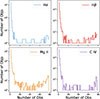 |
Fig. 1. Distribution of sources in our samples by the number of repeated spectroscopic observations. The x-axis shows the number of observations per source, while the y-axis indicates the number of sources with that observation count. Only sources with more than one spectroscopic observation are shown, as those with a single observation are not included in our analysis. |
3. Results
3.1. The overall breathing effect
We first investigated the breathing behavior of the four broad emission lines in their respective samples, using the FWHM as a proxy for the velocity of the line emitting gas. The FWHM of each broad line profile was calculated from the total fitted profile obtained by summing over all broad Gaussian components. To quantify FWHM variability, we computed the difference in Δ(logFWHM) between each epoch and all subsequent epochs for each quasar. For a source with n spectroscopic observations, this yielded n(n − 1)/2 observation pairs.
To characterize the relationship between FWHM and continuum variability, we fit a linear relation y = αx to all observation pairs, accounting for uncertainties in both x and y (denoted as Δx and Δy). The best-fit slope a was obtained by minimizing the following quantity:
 (2)
(2)
where wi denoted the weight assigned to each data point. To avoid the fit being dominated by a small number of quasars with many observations, we assigned weights such that each quasar, rather than each observation pair, contributes equally to the regression (i.e., wi = 1/Npairs for each source).
This approach greatly increased the total number of data points. To robustly estimate the uncertainty in the regression slope, we applied a bootstrap resampling procedure to the parent sample, where sources were resampled as whole units, with all associated observation pairs included in each iteration. The linear slope was then computed for all the observation pairs within each resampled subset. The final slope was defined as the median slope of these resampled subsets, with the 1σ confidence interval defined by the 16th and 84th percentiles. The Spearman R value and its uncertainty were estimated in the same way.
To mitigate contamination from flux calibration uncertainties, we retained only data points where Δlog L exceeds both 0.05 dex and 1.5 times its associated uncertainty, ensuring that the measured continuum changes are likely intrinsic. This filtering criterion was applied consistently in subsequent analyses. The regression slopes for Hα, Hβ and Mg II lines are consistent with 0 (Fig. 2), indicating no significant evidence of breathing in these lines. In contrast, C IV exhibits weak but statistically robust anti-breathing. Interestingly, the Hβ panel in Fig. 2 shows a clear excess of data points in the upper-left and lower-right regions, suggesting that strong breathing is present in a small subset of pairs, even though the sample as a whole shows no average breathing signal. The nature of these outliers is explored further in Sect. 4.2.
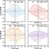 |
Fig. 2. Variation in emission line FWHM as a function of the change in continuum luminosity, for Hα, Hβ, Mg II, and C IV, respectively. No significant breathing effect is detected in Hα, Hβ, or Mg II, with regression slopes consistent with zero. A weak but statistically significant anti-breathing is observed in C IV. In each panel, the solid black line denotes the best-fit regression slope (with the best-fit slope and correlation coefficient R provided), and the error bar at the center represents the median statistical uncertainty of the data points. Interestingly, the Hβ panel shows a clear excess of data points in the upper-left and lower-right regions, suggesting that strong breathing is present in a small subset of pairs, even though the sample as a whole shows no average breathing signal. |
3.2. The timescale dependency of the breathing effect
To assess how the breathing effect varies with timescale, we grouped all data points into bins based on different time intervals. For each pair of observations, we first calculated the rest-frame time interval as Δtrest = Δtobs/(1 + z). Given that the characteristic timescale of BLR breathing can vary significantly across quasars, it is natural to assume that this timescale is related to the size of the BLR. Therefore, when binning by timescale, we normalized the rest-frame time interval by the size of the BLR to account for source-to-source differences, yielding Δtscaled = Δtrest/(RBLR/c), where RBLR was estimated using empirical scaling relations between BLR size and the quasar’s optical continuum luminosity.
For Hα and Hβ, we adopted the RBLR − L relation from Bentz et al. (2013), given in Eq. (3), which uses the monochromatic luminosity at 5100 Å. Although Hα and Hβ are believed to originate from similar regions in the BLR, some studies suggest that the Hα BLR may be slightly more extended (Cho et al. 2023). However, the effect of this difference is likely minor and remains uncertain, so we used the same relation for both lines:
 (3)
(3)
For Mg II, we adopted the scaling relation from Yu et al. (2023), shown in Eq. (4), which uses the 3000 Å continuum luminosity. This relation is consistent with that of Homayouni et al. (2020) within uncertainties but exhibits significantly smaller intrinsic scatter, making it preferable for our analysis:
 (4)
(4)
For C IV, we used the relation from Grier et al. (2019), based on the continuum luminosity at 1350 Å:
 (5)
(5)
After normalizing the time intervals, we assigned weights (wi = 1/Npairs) to each data point such that each quasar, rather than each observation pair, contributes equally to the regression. We then performed linear fits to assess the breathing effect within each time-lag bin using the same methodology described above.
In Fig. 3, we present how the breathing slope varies with tscaled (from top to bottom: Hα, Hβ, Mg II, and C IV ). We find that the Hα, Hβ, and Mg II lines do not exhibit a clear breathing effect at any scaled timescale. While the absence of breathing at tscaled < 1 may be attributed to the impact of the BLR lag, the continued lack of breathing at longer timescales suggests that these lines do not exhibit significant breathing behavior in our sample overall.
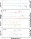 |
Fig. 3. Breathing effect slope as a function of the rest-frame time interval between observations for all four broad emission lines. The bar plot shows the number of observation pairs in each bin, with black error bars indicating the scatter in the pair counts, estimated via bootstrapping. |
In contrast, the C IV line exhibits a clear and timescale-dependent anti-breathing behavior at tscaled > 1. The anti-breathing trend becomes progressively stronger with increasing tscaled, peaks around tscaled ∼ 6, and weakens at longer timescales.
We further examined whether the observed behaviors depend on continuum luminosity or redshift. To this end, we divided each parent sample into two bins based on continuum luminosity (or redshift), ensuring that each bin contains an approximately equal number of quasars. In the higher luminosity (or redshift) bin, the number of observation pairs in the longest time interval bin is consistently smaller, because of the limited temporal baseline. To mitigate the impact of this limitation, we adjusted the selection of time interval bins accordingly. We then repeated the same analysis as performed on the full sample to derive the breathing effect slope as a function of time interval for each subsample. We find no clear dependence of the breathing effect slope on either continuum luminosity or redshift, for all the Hα, Hβ, Mg II, and C IV samples. To better understand the line-specific behaviors, we next discuss the results for each emission line in detail.
4. Discussion
4.1. Hα and Mg II
While earlier studies have found little or no evidence of breathing in broad Hα and Mg II lines (Shen 2013; Homan et al. 2020; Yang et al. 2020; Wang et al. 2020; Ren et al. 2024), our analysis extends this conclusion by showing that the absence of breathing holds across all examined timescales. This reinforces the view that, on average, these two low-ionization lines do not exhibit significant breathing behavior.
A plausible explanation for this lies in the physical structure of the BLR. Photoionization modeling by Guo et al. (2020) suggests that the Hα and Mg II emissions may predominantly arise from gas located near the outer boundary of the BLR. In this scenario, variations in continuum luminosity would not appreciably alter the average radius of the line-emitting region. Consequently, the line widths would remain effectively unchanged, naturally leading to the absence of an observable breathing effect, consistent with our results.
It is important to emphasize, however, that the lack of a breathing effect in these low-ionization lines does not necessarily imply that the corresponding line-emitting gas is not virialized. A key assumption in using the breathing effect to test virial motion is that the intrinsic size-luminosity (R–L) relation follows the same form as the global relation. Yet, this assumption may not always hold. For instance, Peterson et al. (2002) found that in NGC 5548, the Hβ lag scales with the mean continuum level as  , significantly steeper than the global
  relation derived from ensemble studies (Bentz et al. 2013). In the specific case of Hα and Mg II, as argued by Guo et al. (2020), the distance to the line-emitting gas may remain largely unchanged with continuum variations, leading to the absence of an intrinsic R–L relation and, consequently, a lack of breathing effect, even if the gas is gravitationally bound and virialized.
4.2. Hβ
Our analysis reveals a surprising absence of the breathing effect in the broad Hβ line across all timescales (see the second panels of Fig. 3). This is unexpected given that previous reverberation mapping (RM) studies have reported clear breathing behavior in some individual quasars (e.g., Barth et al. 2015), consistent with expectations from virialized BLR motion (Park et al. 2012). Wang et al. (2020) further demonstrated that most quasars in a carefully selected subsample of SDSS-RM quasars (Shen et al. 2015) – those with reliably measured Hβ lags (Grier et al. 2017) – exhibit a significant breathing effect. Our lack of detection in the much broader sample is therefore particularly intriguing.
Closer inspection of the second panel of Fig. 2 reveals a distinct subset of data points in the upper-left and lower-right regions that exhibit strong breathing behavior. These points predominantly originate from SDSS-RM quasars, largely because this population contributes significantly more observation pairs and therefore dominates the sample. To better assess the underlying distribution, we calculated the breathing slope α and its statistical uncertainty αerr for each pair, and identified breathing pairs using a stringent criterion of α < −3αerr. Despite the difference in sample sizes, we find that both RM and non-RM quasars exhibit nearly identical fractions of normal breathing pairs (4.1% vs. 4.3%), suggesting that the RM quasars are not statistically distinct from the non-RM population in this regard.
To benchmark our method and results, we reanalyzed the Hβ sample from Wang et al. (2020) without correcting for the effects of BLR lags. Following their approach, we focused exclusively on SDSS-RM spectroscopic observations from the season of 2014, during which reliable Hβ lags were detected in these sources. The measured values were obtained using the fitting procedure described in Sect. 2.2. As shown in the top panel of Fig. 4, this particular subsample exhibits a typical negative breathing slope across most time-interval bins. Notably, we observe a clear trend of increasing slope magnitude with longer timescales, reaching a value of 0.08 ± 0.05 at the longest timescale (tscaled ≳ 5), which is statistically consistent with the average slope of −0.10 ± 0.04 reported by Wang et al. (2020). This result supports the proposed scenario we introduced in Sect. 1: without correcting for BLR lag effects, the breathing signal can be smeared out at short timescales due to the time delay between the continuum and line emission. However, at longer timescales, the impact of lag smearing diminishes, allowing the underlying breathing effect to reemerge. This further validates our method as a plausible and effective approach for identifying the breathing effect when it is present.
 |
Fig. 4. Same as the second panel of Fig. 3, but for different SDSS-RM quasar subsamples. Top: 31 SDSS-RM quasars with well-measured Hβ lags from Wang et al. (2020), using only 2014 observations. A clear increase in the breathing slope is seen with increasing timescale. Middle: Same SDSS-RM quasar sample as above, but using all available SDSS-RM observations. The breathing trend disappears. Bottom: All RM quasars with more than 20 spectroscopic epochs. No breathing effect is detected either across all timescales. |
However, when we extended the analysis of the same Hβ quasar sample from Wang et al. (2020) to include all available epochs of SDSS-RM spectroscopic observations – not just those from the 2014 season – the breathing trend disappears (see the third panel of Fig. 4). This indicates that the presence of the breathing effect can vary with time, even for the same objects. Notably, the quasars selected by Wang et al. (2020) were chosen specifically because they exhibited detectable Hβ BLR lags during the 2014 monitoring season, and they also showed clear breathing behavior during that period. This suggests a correlation between the detectability of Hβ lags and the manifestation of the breathing effect.
We further note that the 31 Hβ quasars analyzed in Wang et al. (2020) were drawn from a parent sample of 222 SDSS-RM quasars with Hβ spectral coverage (Grier et al. 2017), meaning that the vast majority of SDSS-RM quasars do not have detectable Hβ lags. To place these findings in a broader context, we analyzed all RM quasars in our parent sample. As shown in the bottom panel of Fig. 4, these sources likewise show no average Hβ breathing signal.
To further explore possible intrinsic differences between RM quasars with and without detected Hβ lags, we compared their excess variance, which traces the intrinsic variability of the quasar, and the number of spectroscopic observations during the 2014 season. For each quasar, the excess variance σrms2 is calculated following Vaughan et al. (2003):
 (6)
(6)
where N is the number of spectroscopic measurements, Xi is the observed spectroscopic magnitude measured at 5100 Å,  is the average spectroscopic magnitude (converted from the continuum luminosity), and σi is the uncertainty of each spectroscopic magnitude. As shown in Fig. 5, there is no apparent difference between RM quasars with and without lag detections. Interestingly, those without detected Hβ lags also show no evidence of Hβ breathing during the 2014 season (see the second panel of Fig. 4), further supporting a connection between the detectability of Hβ lags and the manifestation of the Hβ breathing effect.
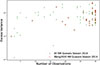 |
Fig. 5. Excess variance as a function of number of spectroscopic observations per SDSS-RM quasar. Red circles represent RM quasars with significant Hβ lag detections from Wang et al. (2020), while green triangles represent all RM quasars in our parent sample, including those without detectable lags. Both samples are based on data from the 2014 monitoring season. There is no clear distinction in either the number of observations or the excess variance between quasars with detected lags and those without. |
Taken together, we find no evidence for an average Hβ breathing effect either among the entire quasar sample or within the full SDSS-RM quasar sample. The breathing effect is detected only in the 31 SDSS-RM quasars reported by Wang et al. (2020) that exhibit significant Hβ lag detections, and only during the 2014 season when the lags were measured. We further examined whether the non-detection of Hβ breathing might depend on the number of spectroscopic epochs per quasar; as shown in Fig. 6, no obvious trend is apparent. These results suggest that while the Hβ breathing effect can indeed manifest when a reliable BLR lag is detected, it is likely not a persistent or universal phenomenon across all epochs or quasars. The detectability of the breathing effect therefore could be be episodic. Future monitoring with longer duration and higher cadence could help to further test and confirm these findings.
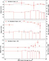 |
Fig. 6. Same as Fig. 4, but for quasars with different number of spectroscopic observations. None of the subsamples exhibits significant breathing effect in Hβ. |
This conclusion is further supported by our finding that only ∼4% of all observation pairs exhibit a normal breathing signature, indicating that for the majority of the time, the Hβ emission line does not show breathing behavior. In fact, a lack of breathing – or even anti-breathing – has been previously reported in individual objects (e.g., Wang et al. 2020) and in different epochs of the same source (e.g., Feng et al. 2024). On longer timescales, Ren et al. (2024) similarly found no significant breathing effect in a sample of extremely variable quasars (EVQs), consistent with our results.
A plausible explanation for the above findings is that, while the broad emission lines respond to variations in the ionizing continuum, the observed optical continuum variability – typically used as a proxy – does not always faithfully trace the ionizing flux. When the optical and ionizing continua are well correlated, both the BLR lag and the breathing effect can be detected. Conversely, if the two continua vary independently, neither phenomenon may be observable. This scenario could explain the lack of breathing detected in our analysis, and suggests that quasars may exhibit correlated optical and ionizing variability only during a small fraction of the time, leading to the episodic appearance of the breathing effect.
Indeed, anomalous responses of broad emission lines to continuum variability have been frequently reported (Goad et al. 2016; Pei et al. 2017; Gaskell et al. 2021; Homayouni et al. 2024). These findings are consistent with recent observational studies (Xin et al. 2020; Sou et al. 2022) and physical models of quasar variability (Cai et al. 2016, 2018, 2020), which increasingly highlight that quasar variability across different bands–from optical to UV and X-ray–is not necessarily well correlated.
4.3. C IV
The anti-breathing trend of the C IV line, as shown in Fig. 2, is consistent with previous findings in the literature (Richards et al. 2002, 2011; Wilhite et al. 2006; Shen et al. 2008; Wang et al. 2020). A plausible interpretation for this behavior invokes a two-component origin of the C IV emission: a broad, rapidly responding component associated with the classical BLR, and a narrower, less variable component likely originating from an intermediate line region or a radiatively driven disk wind. As the continuum luminosity increases, the relative contribution from the broad, reverberating component becomes more prominent, resulting in an overall increase in line width, manifesting as an anti-breathing behavior (e.g., Wang et al. 2020).
In Fig. 3, we further show that this anti-breathing effect is timescale dependent: it strengthens with increasing scaled time separation (tscaled), peaks around tscaled ∼ 6, and declines at longer timescales. This evolution can be naturally understood within the two-component framework. The broad, wing-dominated component requires time to fully respond to continuum variations, which amplifies the anti-breathing signal on intermediate timescales. At longer timescales, the effect weakens, either because the narrower component, initially less responsive, starts to vary with the continuum and dilutes the overall trend, or because the response of the broad component saturates or becomes modified by other processes such as structural evolution or changes in the disk wind launching condition. Extended spectroscopic monitoring will be critical to test these scenarios and to constrain the physical size and variability timescale of the narrow C IV – emitting region.
To further probe the nature of C IV breathing, we examined line dispersion (σ) and several velocity-based line-width tracers (w50, w80, and w90, defined as the velocity differences between the 25th and 75th, 10th and 90th, and 5th and 95th percentiles of the cumulative flux, respectively). These tracers are more sensitive to the line wings than FWHM and are therefore better suited for tracing the broad, reverberating component. As shown in Fig. 7, all four tracers consistently exhibit a normal breathing pattern, i.e., line width decreases with increasing luminosity, in contrast to the anti-breathing behavior seen in FWHM. It is worth noting that using these alternative line-width tracers does not affect the results presented above for other emission lines.
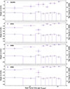 |
Fig. 7. Same as the bottom panel of Fig. 3, but using alternative velocity-based line-width tracers to measure the breathing slopes of the C IV line. We adopted line dispersion σ, as well as the nonparametric widths w50, w80, and w90, which are more sensitive to the line wings and thus better trace the response of the broad, potentially reverberating component. |
The breathing signal in C IV traced by these metrics is strongest at intermediate timescales. At longer timescales, the breathing signal of the wing component also weakens, consistent with the scenario that additional mechanisms, such as changes in the wind structure or the global BLR geometry, modifying the line profile beyond reverberation at longer timescales. These results also highlight the importance of timescale-dependent analyses, and motivate future long-term spectroscopic campaigns to fully characterize the dynamic nature of broad-line variability in quasars.
4.4. Implication on the black hole mass measurement
Different breathing effects across emission lines suggest that intrinsic quasar variability may introduce additional uncertainties in single-epoch black hole mass estimates. The scatter in single-epoch mass measurements is known to correlate with the continuum variability amplitude, and is commonly modeled as following δlog MBH = (2α + 0.5)δlog L, where α is the breathing slope and δlog L represents the variation amplitude of the continuum luminosity (Shen 2013).
In this study, we detect no significant breathing effect in the Hα, Hβ, and Mg II lines across a large quasar sample, while the C IV line shows a timescale-dependent anti-breathing behavior. As we discussed earlier, the absence of a breathing signal does not necessarily imply that the corresponding line-emitting regions are not virialized. Nevertheless, these observational results have direct implications for the accuracy of single-epoch black hole mass estimates. In particular, AGNs with larger variability amplitudes are expected to suffer from larger mass uncertainties due to this effect. Moreover, given that quasar continuum variability at different wavelengths may be poorly correlated (see Sect. 4.2), the actual impact of δlog L on mass estimates may be even more significant than what is inferred from the continuum variability amplitude measured near the wavelength of the emission line itself.
To quantify this effect empirically, we examined our quasars with exactly two spectroscopic observations and compute the black hole mass difference between the two epochs using the standard single-epoch virial mass formula from Shen et al. (2024). We find that the median (90th percentile) mass differences are approximately 0.11 (0.22), 0.16 (0.30), and 0.10 (0.18) dex for Hβ-, Mg II-, and C IV-based estimates, respectively. While these median values are relatively small compared to the typical systematic uncertainty of ∼0.4 dex, which is dominated by contributions from the virial factor uncertainty and R–L relation scatter (e.g., Shen 2013), a small fraction of quasars exhibit mass differences that are comparable to this level when measured across two spectroscopic epochs. Clearly, in the absence of strong breathing effects, our results suggest that while continuum variability (and statistical fluctuations in line width measurements) contribute modestly to the typical scatter in single-epoch black hole mass estimates, they can introduce substantial deviations in a small fraction of quasars.
5. Conclusions
In this work, we performed a comprehensive analysis of the breathing effect–the luminosity-dependent variability of broad emission line widths–in a large sample of quasars with multi-epoch spectroscopy from SDSS DR16. By examining four prominent emission lines (Hα, Hβ, Mg II, and C IV) and quantifying their line width response to continuum luminosity changes over a range of rest-frame time intervals, we aim to understand the physical conditions and temporal characteristics under which the breathing effect arises, and assess its implications for black hole mass estimates. Our main findings are summarized as follows:
-
No breathing effect on average is detected in the Hα, Hβ, or Mg II lines on any rest-frame timescale, suggesting that the widths of these low-ionization lines do not systematically respond to continuum luminosity changes in the majority of quasars.
-
The C IV line shows a clear anti-breathing effect, where the line width increases with continuum luminosity. This behavior is statistically significant and most pronounced at intermediate timescales, while at longer timescales, the trend may be influenced by additional physical processes that affect the C IV profile.
-
For Hβ, which has previously shown breathing in individual reverberation-mapped quasars, we find no significant trend on average. However, the breathing effect can be recovered in quasars with detected BLR lags, but only when restricting the analysis to epochs where the lag is clearly measurable. This suggests that the breathing behaviors could be episodic, likely to be attributed to a weak or variable correlation between the optical and ionizing continua.
-
Using quasars with two spectroscopic epochs, we find that black hole mass estimates typically differ by ∼0.1–0.2 dex, with ∼10% of sources reaching differences of up to 0.3 dex. In the absence of a clear breathing effect, such differences cannot be easily corrected.
These results offer new insights into the complicated nature of BLR breathing effect in quasars and reinforce the need for caution when using single-epoch spectra to estimate black hole masses.
Note that modeling the C IV doublet either as a single blended line or as two individual components (λ1548, λ1550) with appropriate flux ratios yields consistent results.
Acknowledgments
We thank the anonymous referee for the valuable comments and suggestions, which have significantly improved the manuscript. This work was supported by the National Natural Science Foundation of China (grant Nos. 12533006, 12033006 & 12192221) and the Cyrus Chun Ying Tang Foundations.
References
- Barth, A. J., Bennert, V. N., Canalizo, G., et al. 2015, ApJS, 217, 26 [NASA ADS] [CrossRef] [Google Scholar]
- Bentz, M. C., Peterson, B. M., Netzer, H., Pogge, R. W., & Vestergaard, M. 2009, ApJ, 697, 160 [Google Scholar]
- Bentz, M. C., Denney, K. D., Grier, C. J., et al. 2013, ApJ, 767, 149 [Google Scholar]
- Cai, Z.-Y., Wang, J.-X., Gu, W.-M., et al. 2016, ApJ, 826, 7 [NASA ADS] [CrossRef] [Google Scholar]
- Cai, Z.-Y., Wang, J.-X., Zhu, F.-F., et al. 2018, ApJ, 855, 117 [Google Scholar]
- Cai, Z.-Y., Wang, J.-X., & Sun, M. 2020, ApJ, 892, 63 [Google Scholar]
- Cho, H., Woo, J.-H., Wang, S., et al. 2023, ApJ, 953, 142 [Google Scholar]
- Feng, H.-C., Li, S.-S., Bai, J. M., et al. 2024, ApJ, 976, 176 [Google Scholar]
- Gaskell, C. M. 2009, New Astron. Rev., 53, 140 [Google Scholar]
- Gaskell, C. M., Bartel, K., Deffner, J. N., & Xia, I. 2021, MNRAS, 508, 6077 [NASA ADS] [CrossRef] [Google Scholar]
- Goad, M. R., Korista, K. T., De Rosa, G., et al. 2016, ApJ, 824, 11 [NASA ADS] [CrossRef] [Google Scholar]
- Grier, C. J., Trump, J. R., Shen, Y., et al. 2017, ApJ, 851, 21 [NASA ADS] [CrossRef] [Google Scholar]
- Grier, C. J., Shen, Y., Horne, K., et al. 2019, ApJ, 887, 38 [NASA ADS] [CrossRef] [Google Scholar]
- Guo, H., & Gu, M. 2014, ApJ, 792, 33 [Google Scholar]
- Guo, H., Shen, Y., & Wang, S. 2018, Astrophysics Source Code Library [record ascl:1809.008] [Google Scholar]
- Guo, H., Shen, Y., He, Z., et al. 2020, ApJ, 888, 58 [NASA ADS] [CrossRef] [Google Scholar]
- Homan, D., MacLeod, C. L., Lawrence, A., Ross, N. P., & Bruce, A. 2020, MNRAS, 496, 309 [NASA ADS] [CrossRef] [Google Scholar]
- Homayouni, Y., Trump, J. R., Grier, C. J., et al. 2020, ApJ, 901, 55 [Google Scholar]
- Homayouni, Y., Kriss, G. A., De Rosa, G., et al. 2024, ApJ, 963, 123 [Google Scholar]
- Kang, W.-Y., Wang, J.-X., Cai, Z.-Y., & Ren, W.-K. 2021, ApJ, 911, 148 [Google Scholar]
- Kaspi, S., Maoz, D., Netzer, H., et al. 2005, ApJ, 629, 61 [Google Scholar]
- Kaspi, S., Brandt, W. N., Maoz, D., et al. 2021, ApJ, 915, 129 [NASA ADS] [CrossRef] [Google Scholar]
- Korista, K. T., & Goad, M. R. 2004, ApJ, 606, 749 [NASA ADS] [CrossRef] [Google Scholar]
- Lira, P., Kaspi, S., Netzer, H., et al. 2018, ApJ, 865, 56 [NASA ADS] [CrossRef] [Google Scholar]
- Lyke, B. W., Higley, A. N., McLane, J. N., et al. 2020, ApJS, 250, 8 [NASA ADS] [CrossRef] [Google Scholar]
- Park, D., Woo, J.-H., Treu, T., et al. 2012, ApJ, 747, 30 [CrossRef] [Google Scholar]
- Pei, L., Fausnaugh, M. M., Barth, A. J., et al. 2017, ApJ, 837, 131 [NASA ADS] [CrossRef] [Google Scholar]
- Peterson, B. M., & Wandel, A. 2000, ApJ, 540, L13 [NASA ADS] [CrossRef] [Google Scholar]
- Peterson, B. M., Berlind, P., Bertram, R., et al. 2002, ApJ, 581, 197 [NASA ADS] [CrossRef] [Google Scholar]
- Peterson, B. M., Ferrarese, L., Gilbert, K. M., et al. 2004, ApJ, 613, 682 [Google Scholar]
- Ren, W., Wang, J., Cai, Z., & Hu, X. 2024, ApJ, 963, 7 [Google Scholar]
- Richards, G. T., Vanden Berk, D. E., Reichard, T. A., et al. 2002, AJ, 124, 1 [NASA ADS] [CrossRef] [Google Scholar]
- Richards, G. T., Kruczek, N. E., Gallagher, S. C., et al. 2011, AJ, 141, 167 [Google Scholar]
- Shen, Y. 2013, Bull. Astron. Soc. India, 41, 61 [NASA ADS] [Google Scholar]
- Shen, Y., Greene, J. E., Strauss, M. A., Richards, G. T., & Schneider, D. P. 2008, ApJ, 680, 169 [Google Scholar]
- Shen, Y., Brandt, W. N., Dawson, K. S., et al. 2015, ApJS, 216, 4 [Google Scholar]
- Shen, Y., Horne, K., Grier, C. J., et al. 2016, ApJ, 818, 30 [NASA ADS] [CrossRef] [Google Scholar]
- Shen, Y., Grier, C. J., Horne, K., et al. 2024, ApJS, 272, 26 [NASA ADS] [CrossRef] [Google Scholar]
- Sou, H., Wang, J.-X., Xie, Z.-L., Kang, W.-Y., & Cai, Z.-Y. 2022, MNRAS, 512, 5511 [Google Scholar]
- Vaughan, S., Edelson, R., Warwick, R. S., & Uttley, P. 2003, MNRAS, 345, 1271 [Google Scholar]
- Wang, S., Shen, Y., Jiang, L., et al. 2020, ApJ, 903, 51 [NASA ADS] [CrossRef] [Google Scholar]
- Wilhite, B. C., Vanden Berk, D. E., Brunner, R. J., & Brinkmann, J. V. 2006, ApJ, 641, 78 [Google Scholar]
- Woltjer, L. 1959, ApJ, 130, 38 [NASA ADS] [CrossRef] [Google Scholar]
- Xin, C., Charisi, M., Haiman, Z., & Schiminovich, D. 2020, MNRAS, 495, 1403 [CrossRef] [Google Scholar]
- Yang, Q., Shen, Y., Chen, Y.-C., et al. 2020, MNRAS, 493, 5773 [Google Scholar]
- Yu, Z., Martini, P., Penton, A., et al. 2023, MNRAS, 522, 4132 [NASA ADS] [CrossRef] [Google Scholar]
All Figures
|
Fig. 1. Distribution of sources in our samples by the number of repeated spectroscopic observations. The x-axis shows the number of observations per source, while the y-axis indicates the number of sources with that observation count. Only sources with more than one spectroscopic observation are shown, as those with a single observation are not included in our analysis. |
| In the text | |
|
Fig. 2. Variation in emission line FWHM as a function of the change in continuum luminosity, for Hα, Hβ, Mg II, and C IV, respectively. No significant breathing effect is detected in Hα, Hβ, or Mg II, with regression slopes consistent with zero. A weak but statistically significant anti-breathing is observed in C IV. In each panel, the solid black line denotes the best-fit regression slope (with the best-fit slope and correlation coefficient R provided), and the error bar at the center represents the median statistical uncertainty of the data points. Interestingly, the Hβ panel shows a clear excess of data points in the upper-left and lower-right regions, suggesting that strong breathing is present in a small subset of pairs, even though the sample as a whole shows no average breathing signal. |
| In the text | |
|
Fig. 3. Breathing effect slope as a function of the rest-frame time interval between observations for all four broad emission lines. The bar plot shows the number of observation pairs in each bin, with black error bars indicating the scatter in the pair counts, estimated via bootstrapping. |
| In the text | |
|
Fig. 4. Same as the second panel of Fig. 3, but for different SDSS-RM quasar subsamples. Top: 31 SDSS-RM quasars with well-measured Hβ lags from Wang et al. (2020), using only 2014 observations. A clear increase in the breathing slope is seen with increasing timescale. Middle: Same SDSS-RM quasar sample as above, but using all available SDSS-RM observations. The breathing trend disappears. Bottom: All RM quasars with more than 20 spectroscopic epochs. No breathing effect is detected either across all timescales. |
| In the text | |
|
Fig. 5. Excess variance as a function of number of spectroscopic observations per SDSS-RM quasar. Red circles represent RM quasars with significant Hβ lag detections from Wang et al. (2020), while green triangles represent all RM quasars in our parent sample, including those without detectable lags. Both samples are based on data from the 2014 monitoring season. There is no clear distinction in either the number of observations or the excess variance between quasars with detected lags and those without. |
| In the text | |
|
Fig. 6. Same as Fig. 4, but for quasars with different number of spectroscopic observations. None of the subsamples exhibits significant breathing effect in Hβ. |
| In the text | |
|
Fig. 7. Same as the bottom panel of Fig. 3, but using alternative velocity-based line-width tracers to measure the breathing slopes of the C IV line. We adopted line dispersion σ, as well as the nonparametric widths w50, w80, and w90, which are more sensitive to the line wings and thus better trace the response of the broad, potentially reverberating component. |
| In the text | |
Current usage metrics show cumulative count of Article Views (full-text article views including HTML views, PDF and ePub downloads, according to the available data) and Abstracts Views on Vision4Press platform.
Data correspond to usage on the plateform after 2015. The current usage metrics is available 48-96 hours after online publication and is updated daily on week days.
Initial download of the metrics may take a while.