| Issue |
A&A
Volume 704, December 2025
|
|
|---|---|---|
| Article Number | A298 | |
| Number of page(s) | 18 | |
| Section | Stellar structure and evolution | |
| DOI | https://doi.org/10.1051/0004-6361/202556787 | |
| Published online | 17 December 2025 | |
A magnetic field study of two fast-rotating, radio-bright M dwarfs
StKM 1-1262 and V374 Peg
1
Leiden Observatory, Leiden University, PO Box 9513 2300 RA Leiden, The Netherlands
2
Institut de Recherche en Astrophysique et Planétologie, Université de Toulouse, CNRS, IRAP/UMR 5277, 14 avenue Edouard Belin, F-31400 Toulouse, France
3
Center for Astrophysics | Harvard & Smithsonian, 60 Garden Street, Cambridge, MA 02138, USA
4
ASTRON, Netherlands Institute for Radio Astronomy, Oude Hoogeveensedijk 4, Dwingeloo 7991 PD, The Netherlands
5
Anton Pannekoek Institute for Astronomy, University of Amsterdam, Science Park 904, 1098 XH Amsterdam, The Netherlands
6
Laboratoire Univers et Particules de Montpellier, Université de Montpellier, CNRS, F-34095 Montpellier, France
7
School of Physics and Astronomy, University of St Andrews, North Haugh, St Andrews, Fife KY16 9SS, Scotland
8
Canada-France-Hawaii Telescope, 65-1238 Mamalahoa Hwy, Kamuela, HI 96743, USA
9
Lowell Observatory, 1400 W. Mars Hill Rd. Flagstaff, AZ 86001, USA
10
Kapteyn Astronomical Institute, University of Groningen, PO Box 800 9700 AV Groningen, The Netherlands
★ Corresponding author: This email address is being protected from spambots. You need JavaScript enabled to view it.
Received:
8
August
2025
Accepted:
2
November
2025
Abstract
Context. Radio observations at low frequencies are sensitive to the magnetic activity of stars and the plasma environment surrounding them, so one can scrutinize the conditions under which stellar space weather develops and impacts exoplanets. The accurate interpretation of the processes underlying the radio signatures requires a detailed characterisation of stellar magnetism.
Aims. We study two M dwarfs, namely StKM 1-1262 (M0 type, Prot = 1.24 d) and V374 Peg (M4 type, Prot = 0.4455 d), which were detected recently with the LOw Frequency ARray (LOFAR). StKM 1-1262 exhibited the typical signature of a type-II radio burst, potentially resulting from a coronal mass ejection event. V374 Peg manifested low-frequency radio emission with high brightness temperature and low degree of polarisation, suggesting an electron-cyclotron maser instability emission mechanism. In this work, we provide recent observational constraints on the magnetic field of both stars.
Methods. We analysed spectropolarimetric observations of these M dwarfs, collected with the SpectroPolarimètre InfraRouge (SPIRou). Firstly, we refined the stellar parameters, such as effective temperature, surface gravity, and metallicity, and measured the average surface magnetic flux via modelling of Zeeman broadening in unpolarised spectra. We then applied Zeeman-Doppler imaging to least-squares deconvolution line profiles in circular polarisation to reconstruct their large-scale magnetic fields. We also reconstructed a brightness map for the two stars using Doppler imaging.
Results. StKM 1-1262 has a total, unsigned magnetic field of 3.53 ± 0.06 kG on average, and the large-scale magnetic field topology is predominantly poloidal, dipolar and moderately axisymmetric, with an average strength of 300 G. V374 Peg has an unsigned magnetic field of 5.46 ± 0.09 kG, and the large-scale field is poloidal, dipolar and axisymmetric, with an average strength of 800 G. For StKM 1-1262, we found a strong (Pearson ρ = −0.96) anti-correlation between the total magnetic field and the effective temperature, which is reminiscent of the tight link between small-scale magnetic fields and surface inhomogeneities. For V374 Peg, we found a moderate (ρ = −0.43) anti-correlation, possibly due to a more even distribution of surface features.
Conclusions. The large-scale magnetic field topology of StKM 1-1262 is similar to other stars with similar fundamental parameters like mass and rotation period, and the brightness map features one dark spot, which is responsible for the rotational modulation of the total magnetic field and the retrieved effective temperature. For V374 Peg, the magnetic topology and the brightness map are similar to previous reconstructions, indicating a temporal stability of approximately 14-yr.
Key words: techniques: polarimetric / stars: activity / stars: magnetic field
© The Authors 2025
 Open Access article, published by EDP Sciences, under the terms of the Creative Commons Attribution License (https://creativecommons.org/licenses/by/4.0), which permits unrestricted use, distribution, and reproduction in any medium, provided the original work is properly cited.
This article is published in open access under the Subscribe to Open model. This email address is being protected from spambots. You need JavaScript enabled to view it. to support open access publication.
1. Introduction
A central goal of exoplanetology is to find Earth-like planets that potentially host life. According to the canonical definition, assessing the potential habitability of a planet requires knowledge about the distance (or insolation) of the planet from the star (Kasting et al. 1993; Kopparapu 2013). However, this is a first-order assessment, and additional details such as the stellar magnetic field (Driscoll & Bercovici 2013), the planetary volcanic and tectonic activity (Lenardic et al. 2016; Seales & Lenardic 2021), the distribution of oceans (Cockell et al. 2016), the asteroid impacts (Childs et al. 2022), and the binarity of the host star (Jaime et al. 2014; Cuntz 2015; Cuntz & Wang 2020) are needed to obtain a comprehensive definition of habitability. The space weather and radiation environment in which exoplanets orbit is also crucial in this context (Vidotto et al. 2013; Airapetian et al. 2017, 2020). X-ray and UV radiation, for example, can drive atmospheric escape and alter its chemical constituents, ultimately shaping the evolution of planetary atmospheres (Lammer et al. 2003; Penz & Micela 2008; Owen & Jackson 2012; Rugheimer et al. 2015; Carolan et al. 2019; Van Looveren et al. 2024).
Coronal mass ejections (CMEs) are expulsions of hot coronal plasma and magnetic field into the heliosphere, with speeds ranging from 100 to 2000 km s−1 (Nindos et al. 2008; Webb & Howard 2012). They represent a major constituent of space weather in the Solar System and a continuous exposure is expected to lead to the erosion of planetary atmospheres over time (Lammer et al. 2007; Khodachenko et al. 2007). Similar effects are expected on other stars (Lammer 2013; Cherenkov et al. 2017), but there has yet to be an unambiguous detection of an extrasolar CME, despite a substantial observational effort (e.g. Crosley et al. 2016; Crosley & Osten 2018). The incidence and energetics of these phenomena are thus not constrained empirically, which prevents us from assessing the habitability of other systems in a comprehensive manner.
Radio observations of stellar systems allow one to investigate stellar magnetic activity and the space weather conditions of extrasolar planets (see Callingham et al. 2024, and references therein). Observing a type II radio burst represents a detection of plasma radial motion away from the star, because electrons are accelerated by shocks at the leading edges of outward-moving CMEs, which generate the typical frequency sweep (Cane et al. 2002; Gopalswamy et al. 2008; Osten & Wolk 2017; Majumdar et al. 2021). A type II radio burst is thus a ‘smoking gun’ signature of CMEs, but it has been elusive for stars other than the Sun.
Another puzzle coming from radio observations of stellar systems concerns the low-frequency radio emission detected from both active and quiescent M dwarfs within the LOFAR Two-meter Sky Survey (LoTSS Shimwell et al. 2017, 2022). Specifically, these observations unravelled a population of M1-M6 dwarfs manifesting coherent, low-frequency (on the order of MHz) radio emission that is highly circularly polarised (≥60%), with high brightness temperature (> 1012 K) (Callingham et al. 2021). To explain these findings, there are two main categories of processes: plasma emission and electron-cyclotron maser instability (ECMI) emission. The former occurs when flares and CMEs inject hot plasma into colder plasma (Dulk et al. 1985; Matthews 2019), and is correlated with stellar magnetic activity (McLean et al. 2012; Villadsen & Hallinan 2019; Callingham et al. 2021). The M dwarfs detected within the LOFAR Two-metre Sky Survey (LoTSS) span various activity levels, suggesting that the radio emission may not be only activity-driven, which finds support from analyses of flare activity conducted with the Transiting Exoplanet Survey Satellite (TESS; Ricker et al. 2014), as shown by Pope et al. (2021).
For ECMI-driven emission (Wu & Lee 1979; Treumann 2006), the scenario sees an acceleration of electrons towards the star, powering auroral processes similar to Jupiter (Zarka 1998). The first possibility is that, at a certain distance from the star, the stellar magnetic field cannot impose co-rotation of the surrounding plasma. This breakdown of co-rotation generates a lag between the plasma disk and the star’s magnetosphere, and ultimately a current system that accelerates electrons towards the star (Nichols et al. 2012; Pineda et al. 2017; Marques et al. 2017). A second possibility translates the Jupiter interaction with its moon Io into a star-planet one, for which a planet orbits within the Alfvén surface of the host star and perturbs or reconnects with the stellar magnetic field, driving electron acceleration (Lazio et al. 2004; Zarka 2007; Turnpenney et al. 2018; Vidotto et al. 2019; Vedantham et al. 2020). Although there are candidates for star-planet interactions, no exoplanet has been conclusively detected yet via low-frequency radio emission (Lynch et al. 2018; Vedantham et al. 2020; Pope et al. 2021; Turner et al. 2021; Pérez-Torres et al. 2021).
Considering the sensitivity of radio observations to the plasma environment around a star, interpreting such observations requires an accurate model of the stellar magnetic environment and wind (e.g. Vidotto et al. 2014; Kavanagh et al. 2019, 2021, 2022; Alvarado-Gómez et al. 2022; Elekes & Saur 2023; Peña-Moñino et al. 2024). In turn, this type of model is determined by our knowledge of the magnetic field of the star, whose large-scale configuration can be reconstructed from spectropolarimetric time series via Zeeman-Doppler imaging (ZDI; Semel 1989; Donati & Brown 1997). Over the years, ZDI has been applied extensively, revealing a variety of field geometries for low-mass stars, as well as their temporal evolution (e.g. Petit et al. 2005; Donati et al. 2008; Morin et al. 2008b, 2010; Hébrard et al. 2016; Kochukhov & Lavail 2017; Lavail et al. 2018; Folsom et al. 2018; Bellotti et al. 2023b, 2024).
Here, we analyse recent spectropolarimetric observations of two stars, StKM 1-1262 and V374 Peg, and characterise their large-scale magnetic field. These two stars were detected within the LoTSS survey (Tasse et al. 2021; Yiu et al. 2024). StKM 1-1262 is an early M dwarf for which a candidate type II radio burst was detected as an isolated event, with the characteristic frequency sweep of a typical solar type II burst but more than four orders of magnitude radio luminous (Callingham et al. 2025). The constraint of the large-scale magnetic field geometry in the current work is used to determine whether a CME could have sufficient kinetic energy to escape the large-scale field and could drive a super-Alfvénic shock (Callingham et al. 2025). V374 Peg is an active, fully convective mid-M dwarf known to exhibit frequent flares (Korhonen et al. 2010; Vida et al. 2016), a strong (∼1 kG), poloidal, and axisymmetric large-scale magnetic field (Morin et al. 2008a), and a powerful wind (Vidotto et al. 2011). Radio emission from V374 Peg was detected with the Very Large Array in a frequency band of 4–8 GHz (Hallinan et al. 2009), and the modulation of the radio light curve due to stellar rotation was fit by Llama et al. (2018), using an ECMI-driven model. Additional radio observations were obtained within the LoTSS survey (120–168 MHz) in 2018 and more recently in 2024, bracketing our spectropolarimetric observations. The reconstructed large-scale magnetic field in this work will then be used as a boundary condition to simulate the stellar environment of V374 Peg, and better understand which ECMI mechanism is powering the observed low-frequency radio emission in a follow-up study.
This paper is structured as follows. In Sect. 2 we describe the spectropolarimetric dataset. In Sect. 3 we outline the modelling of Zeeman broadening and intensification of unpolarised spectra to measure the total, unsigned magnetic field intensity. In Sects. 4 and 5 we describe the analysis of circular polarisation spectra to measure the longitudinal magnetic field and to reconstruct the large-scale magnetic field geometry by means of ZDI, respectively. We then show the reconstruction of the brightness maps of StKM 1-1262 and V374 Peg with Doppler imaging in Sect. 6. Finally, we draw our conclusions in Sect. 7.
2. Observations
The observations we analyse in this work were obtained in circular polarisation mode with the SpectroPolarimètre InfraRouge (SPIRou Donati et al. 2020), the stabilised high-resolution near-infrared spectropolarimeter mounted on the 3.6 m Canada–France–Hawaii Telescope (CFHT), atop Maunakea, Hawaii. SPIRou operates between 0.96 and 2.5 μm (YJHK bands) at a spectral resolving power of R ∼ 70 000. Optimal extraction of spectra in unpolarised (Stokes I) and circularly polarised (Stokes V) light was carried out with A PipelinE to Reduce Observations (APERO), a fully automatic reduction package installed at CFHT (Cook et al. 2022). The observations of both stars were reduced with APERO v0.7.288. The journal of observations is given in Table A.1 and Table A.2.
StKM 1-1262 was observed for 17 nights between January and March 2024, spanning a period of 41 days. We recorded a signal-to-noise ratio (S/N) at 1650 nm per spectral element between 210 and 278, with a mean of 246. Two observations (23 and 28 February) did not reach enough S/N to produce meaningful Stokes V LSD profiles (see Sect. 4), so they were discarded. V374 Peg was observed 55 times between 14 and 23 August 2021. The recorded S/N oscillated between 86 and 189, with an average of 162. In Table 1, we provide the fundamental stellar aparameters derived and used in this work for both stars.
Properties of StKM 1-1262 and V374 Peg.
The observations of StKM 1-1262 and V374 Peg are phased according to the ephemeris
 (1)
(1)
In the formula, HJD0 is the reference heliocentric Julian date (2460330.1563 for StKM 1-1262 and 2459440.7902 for V374 Peg), Prot is the stellar rotation period (see Table 1), and ncyc is the number of rotation cycles.
3. Total magnetic field and atmospheric characterisation
We estimated the average small-scale magnetic field strength at the stellar surface of StKM 1-1262 and V374 Peg, following the approach described in Cristofari et al. (2023a,b). Our process relies on synthetic spectra computed from MARCS model atmospheres (Gustafsson et al. 2008) with ZeeTurbo (Cristofari et al. 2023a), a tool built from the Turbospectrum (Plez 2012) and Zeeman (Landstreet 1988; Wade et al. 2001; Folsom et al. 2016) codes. Specifically, we computed a grid of synthetic spectra for different sets of atmospheric parameters, with Teff ranging from 3200 to 4400 K in steps of 100 K, log g ranging from 4.0 to 5.0 dex in steps of 0.5 dex, and [M/H] ranging from −0.75 to 0.75 dex in steps of 0.25 dex. The chosen ranges are wide enough to encompass typical parameters for M dwarfs and act as uniform priors. For each set of atmospheric parameters, we computed spectra with different magnetic field intensities, ranging from 0 to 10 kG in steps of 2 kG, assuming that the magnetic field is radial in all points of the photosphere.
A model of the observed spectrum is obtained with a linear combination of the spectra computed for the different magnetic field intensities, so that S = ∑ifiSi, with S the model spectrum, Si the spectrum computed for a i kG field, and fi the associated filling factor. We rely on a Markov chain Monte Carlo (MCMC) process to derive the set of atmospheric parameters, filling factors, and projected rotational velocity (veq sin i) leading to the best fit to the data and to estimate formal error bars (see also Cristofari et al. 2023a,b, for more details). Our method is inherently sensitive to systematics, which is not fully reflected by our formal error bars. Following Cristofari et al. (2022), we inflate the error bars by quadratically adding 30 K, 0.05 dex, and 0.10 dex to Teff, log g, and [M/H], respectively.
For both stars, we begin by applying our process to template spectra obtained by taking the median of all available spectra. For StKM 1-1262, our process yields Teff = 3933 ± 31 K, log g = 4.65 ± 0.05 dex, [M/H] = −0.07 ± 0.10 dex, and veq sin i = 25.04 ± 0.10 km s−1. For V374 Peg, our analysis yields Teff = 3228 ± 30 K, log g = 4.72 ± 0.05 dex, [M/H] = 0.07 ± 0.10 dex, and veq sin i = 36.73 ± 0.17 km s−1. Our atmospheric estimates are reported in Table 1.
For StKM 1-1262, our best fit on the template spectrum yields an average small-scale magnetic field of ⟨BI⟩ = 3.53 ± 0.06 kG, with most of the magnetic intensity distributed on the 2 and 4 kG components (∼87% of the total magnetic flux; see Fig. 1). The value ⟨BI⟩ = 3.53 kG is consistent with that obtained for fast-rotating, early M dwarfs, such as OT Ser (⟨BI⟩ = 3.2 kG; Shulyak et al. 2019) and YY Gem (⟨BI⟩ = 3.2 − 3.4 kG; Kochukhov & Shulyak 2019). For V374 Peg, our process yields an average small-scale magnetic field of ⟨BI⟩ = 5.46 ± 0.09 kG. The distribution of filling factors shows more contribution from the higher components, with the 4, 6 and 8 kG components accounting for 90% of the total magnetic flux. In contrast to StKM 1-1262, the 2 kG component only amounts to 4% of the magnetic flux of V374 Peg (see Fig. 1).
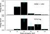 |
Fig. 1. Distribution of magnetic flux on different magnetic components. The top panel refers to StKM 1-1262 and the bottom panel to V374 Peg. |
For each star, we repeat our process, this time analysing each individual spectrum and fixing the values of log g and [M/H] to those listed in Table 1. This approach allows us to simultaneously explore the temporal variations of ⟨BI⟩ and temperature. Figure 2 shows ⟨BI⟩ computed for each observation of StKM 1-1262 and V374 Peg, colour-coded by the associated value of Teff.
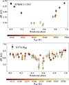 |
Fig. 2. Total magnetic field measurements of StKM 1-1262 and V374 Peg as a function of rotational phase. The data points are colour-coded with the effective temperature obtained from spectral modelling (see Sect. 3). The rotational phases are computed according to Eq. (1), using the stellar rotation period listed in Table 1. |
For StKM 1-1262, the ⟨BI⟩ range from ∼4.50 to ∼3.25 kG, and exhibit an evident modulation at the stellar rotation period of 1.24 d. We note a clear anti-correlation between ⟨BI⟩ and Teff (Pearson correlation coefficient ρ = −0.96). Specifically, we observe ⟨BI⟩ to be highest around phase 0.0, when the retrieved Teff is lowest. This behaviour was already captured for the active M dwarfs AU Mic (Artigau et al. 2024), EV Lac, and DS Leo (Cristofari et al. 2025). As we describe from Doppler imaging in Sect. 6, such behaviour tracks the presence of a starspot or a group of starspots, which are cooler than the quiet photosphere.
We further use the anti-correlation between ⟨BI⟩ and temperature to estimate the spot coverage of StKM 1-1262. We fit a line ⟨BI⟩ as a function of temperature, which yields a slope of −54 ± 5 K kG−1 and an intercept of 4139 ± 18 K (see also Fig. B.1). We attribute the intercept of this fit to the temperature of the quiet photosphere (Tmax). Following the relation of Berdyugina (2005), we derive a spot temperature for StKM 1-1262 of Tspot = 3303 ± 14 K. Given a temperature T = 3933 K (see also Table 1), we then compute the fraction of stellar surface occupied by spots f, such that
 (2)
(2)
Injecting the effective temperature obtained for StKM 1-1262 into Eq. (2), we derive a spot coverage of about f = 25%.
For V374 Peg, no clear rotational modulation of ⟨BI⟩ is observed, which can be attributed to the lower S/N of the individual spectra, making the fitting procedure more challenging. We find a moderate anti-correlation (Pearson correlation coefficient ρ = −0.43) between our temperature and the ⟨BI⟩ measurements, with a linear fit yielding a slope of −37 ± 7 K kG−1 and an intercept of 3461 ± 43 K. Based on the relation of Berdyugina (2005), we derive a spot temperature Tspot = 2979 ± 15, and deduce a spot coverage of about 48%.
4. Longitudinal magnetic field
We computed mean line profiles using least-squares deconvolution (LSD; Donati et al. 1997; Kochukhov et al. 2010), and in particular the Python LSDpy package (Folsom et al. 2025)1. Both the Stokes I and V spectra are deconvolved with a line list, to obtain individual, high S/N profiles summarising the properties of hundreds of spectral lines. The line list contains absorption lines in the stellar spectrum and with the associated line features, such as depth and sensitivity to the Zeeman effect (commonly known as the Landé factor geff). For our stars, we used a synthetic line list corresponding to a local thermodynamic equilibrium model (Gustafsson et al. 2008), characterised by log g = 5.0 [cm s−2], vmicro = 1 km s−1, and Teff = 3500 K. The adopted line list contains 1400 atomic photospheric lines between 950–2600 nm with depth larger than 3% the continuum level. The masks were synthesised using the Vienna Atomic Line Database2 (VALD, Ryabchikova et al. 2015). We set the LSD normalisation wavelength and geff to 1700 nm and 1.2, respectively.
We computed the disk-integrated, line-of-sight component of the large-scale magnetic field following Donati et al. (1997). We used the general formula as in Cotton et al. (2019),
 (3)
(3)
where λ0 and geff are the normalisation wavelength and Landé factor of the LSD profiles, V is the LSD Stokes profile in circular polarisation, I is the LSD Stokes profile in unpolarised light, Ic is the continuum level, v is the radial velocity associated with a point in the spectral line profile in the star’s rest frame, h is Planck’s constant, and μB is the Bohr magneton. To express it as in Rees & Semel (1979) and Donati et al. (1997), one can use hc/μB = 0.0214 Tm, where c is the speed of light in m s−1.
For StKM 1-1262, the computation of Bl was carried out within ±55 km s−1 from line centre at −3.9 km s−1 for both Stokes I and V LSD profiles. As shown in Fig. 3, the values range between −127 and −8 G, with a median value of −74 G and a median error bar of 12 G. The error bars are estimated from the formal propagation of Eq. (3). The phase-folded Bℓ time series does not feature an evident modulation at the stellar rotation period, but rather higher frequency variations around the first harmonic of Prot. When the Bℓ data points are colour-coded based on Teff in a similar manner to Fig. 2, we do not observe a correlation (Pearson ρ = 0.01; see also Fig. B.1).
 |
Fig. 3. Longitudinal magnetic field measurements of StKM 1-1262 and V374 Peg. The panels show Bℓ as a function of rotational phase for StKM 1-1262 and V374 Peg. The rotational phases are computed according to Eq. (1), using the rotational period listed in Table 1. |
For V374 Peg, we set an integration range of ±80 km s−1 from line centre at −3.0 km s−1, and we found values between 117 and 680 G, with a median of 330 G and a median error bar of 50 G (see Fig. 3). The modulation of the Bℓ time series sees an increase around phase 0.3 and a decrease around phase 0.8, but the values are always positive. This can indicate a tilted dipolar configuration of the large-scale field, as will be explained in Sect. 5. When colour-coded by Teff, the Bℓ data points do not reveal any evident correlation (Pearson ρ = −0.08), as also shown in Fig. B.1.
Our range of Bℓ measurements are consistent with previous ESPaDOnS observations performed by Morin et al. (2008a), as shown in Fig. 4. Their observations in August 2005, August 2006, and September 2009 resulted in average Bℓ values of 338 G, 309 G, and 307 G. Combined with our observations, we do not see significant variations in the mean and range of Bℓ values, potentially suggesting that the large-scale magnetic field has remained stable.
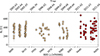 |
Fig. 4. Long-term measurements of V374 Peg’s longitudinal magnetic field. The leftmost epochs (coloured with light brown) represent the August 2005, August 2006, and September 2009 time series analysed by Morin et al. (2008a). The rightmost (dark brown) time series corresponds to the data analysed in this work. |
5. Magnetic field topology
The characterisation of the large-scale magnetic field of StKM 1-1262 and V374 Peg was performed with ZDI (Semel 1989; Donati & Brown 1997). The algorithm compares observed and model Stokes V LSD profiles iteratively, fitting the spherical harmonics coefficients αℓ, m, βℓ, m, and γℓ, m (with ℓ and m the degree and order of the mode, respectively), until they match within a target reduced χ2. Because the inversion problem is poorly posed, a maximum-entropy regularisation scheme is applied to obtain the field map compatible with the data and with the lowest information content (for more details see Skilling & Bryan 1984; Donati & Brown 1997). The magnetic field vector is modelled as the sum of a poloidal and a toroidal component, which are both expressed with spherical harmonics formalism (Lehmann & Donati 2022). We used the python implementation zdipy, with the inclusion of the Unno-Rachkovsky solutions to polarised radiative transfer equations (see Folsom et al. 2018; Bellotti et al. 2024), and the filling factor formalism of Morin et al. (2008b).
The parameters of the Unno-Rachkovsky models (see e.g. del Toro Iniesta 2003; Landi Degl’Innocenti & Landolfi 2004) are the Gaussian width (wG), the Lorentzian width (wL), the ratio of the line to continuum absorption coefficients (η0), and the slope of the source function in the Milne-Eddington atmosphere (β). More information on their implementation in the zdipy code can be found in Erba et al. (2024) and Bellotti et al. (2024). We performed a χ2 minimisation between synthetic and observed Stokes I profiles for a grid of parameters, in order to find the set of parameters that best represents our observations. For StKM 1-1262, we found wG = 9.4 km s−1, wL = 8.0 km s−1, and η0 = 13.0; for V374 Peg, we found wG = 9.0 km s−1, wL = 10.0 km s−1, and η0 = 12.2. The value of β is fixed to 0.25 (for more details, see Erba et al. 2024; Bellotti et al. 2024). The filling factors fI and fV represent the fraction of the cell of the stellar surface grid covered by magnetic regions and magnetic regions producing net circular polarisation, respectively (Morin et al. 2008b; Kochukhov 2021). We attempted to constrain such parameters with a χ2 minimisation but the results were inconclusive, so we fixed both filling factors to 1.0 for both stars.
5.1. Stellar input parameters
The ZDI reconstruction requires physical and geometrical parameters of the star, such as inclination, projected equatorial velocity veq sin i, rotation period, differential rotation rate, limb- darkening coefficient, and maximum degree of spherical harmonics decomposition (ℓmax). The linear limb-darkening coefficient was fixed at 0.2, the value corresponding to the H band observations (Claret & Bloemen 2011).
For veq sin i, we set the values obtained from the spectral fitting procedure (see Sect. 3), namely 25.04 km s−1 for StKM1 1-1262 and 36.73 km s−1 for V374 Peg. The value of veq sin i determines the attainable spatial resolution encapsulated in ℓmax (e.g. Morin et al. 2008a). We conservatively set ℓmax to 10 for the two stars, since most of the magnetic energy is stored in the ℓ ≤ 7 modes.
We attempted a differential rotation search for both stars as described in Petit et al. (2002) but the results were inconclusive, so we assumed solid body rotation. The rotation period of StKM 1-1262 was estimated to be 1.240 ± 0.003 d from TESS photometry (Colman et al. 2024), and for V374 Peg we adopted a value of 0.4455 d (see Morin et al. 2008a). All these values are summarised in Table 1.
Finally, we estimated the inclination of the star, comparing the stellar radius available in the literature with the value obtained geometrically from rotation period and veq sin i. Formally, R sin i = Protveq sin i/50.59, where the denominator accounts for the unit conversion of the variables involved (Prot in d, veqsin(i) in km s−1, and R in R⊙). For StKM 1-1262, we found R sin i = 0.633 ± 0.006 R⊙ while Kervella et al. (2022) reported R = 0.630 R⊙, indicating that the viewing angle of the star is likely equator-on (i.e. 90°). As input for ZDI, we assumed 70° to prevent mirroring effects between the north and south hemispheres of the star. For V374 Peg, we adopted a value of 70° consistent with Morin et al. (2008a).
5.2. Reconstruction
The Stokes V profiles of StKM 1-1262 and their ZDI models are shown in Fig. C.1 and the ZDI map is shown in Fig. 5. We fitted the observed Stokes V LSD profiles down to χr2 = 1.0. As reported in Table 2, the large-scale magnetic geometry is predominantly poloidal, with a strong dipolar component accounting for 75% of the poloidal magnetic energy and also a significant (20%) quadrupolar component. The toroidal field is also substantial, containing 13% of the magnetic energy. The magnetic field is tilted, with only 47% of the total energy stored in the axisymmetric modes (that is, m = 0). This mainly follows the fact that the poloidal component is non-axisymmetric (41%), whereas the toroidal component is axisymmetric (82%). The average magnetic field strength is 300 G.
Properties of the magnetic maps.
The Stokes V profiles of V374 Peg are shown in Fig. C.3 and the ZDI map is shown in Fig. 5. We fitted the observed Stokes V LSD profiles to a χr2 of 1.0. The large-scale magnetic geometry is predominantly poloidal (99%), dipolar (97%), and axisymmetric (92%). The average magnetic field strength is 780 G (see Table 2).
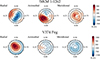 |
Fig. 5. Reconstructed large-scale magnetic field maps in flattened polar view. StKM 1-1262 is shown in the top row and V374 Peg in the bottom row. From the left, the radial, azimuthal, and meridional components of the magnetic field vector are illustrated. Concentric circles represent different stellar latitudes: −30 °, +30 °, and +60 ° (dashed lines), as well as the equator (solid line). The radial ticks are located at the rotational phases when the observations were collected. The rotational phases are computed with Eq. (1), using the first observation of each individual epoch (see Table A.1). The colour bar indicates the polarity and strength (in G) of the magnetic field. |
6. Doppler imaging
Using the time series of Stokes I LSD profiles, we applied Doppler imaging to reconstruct a brightness image of the surface of StKM 1-1262 and of V374 Peg. The principle of the technique is based on the distortions that surface inhomogeneities induce on the shape of spectral lines. Because of the Doppler effect, there is a correlation between the location of the spectral distortion on the profile and the location of the inhomogeneity on the stellar surface. The occurrence of a distortion at a certain time yields information on the longitude of the surface inhomogeneity, while the extent of the distortion across the profile provides the latitude of the spot. Therefore, by monitoring the temporal modulation of such distortions, one can retrieve a 2D brightness map (Deutsch 1957; Vogt & Penrod 1983; Rice et al. 1989).
The longitudinal resolution of the reconstructed map scales with veq sin i (e.g. Hussain et al. 2009; Morin et al. 2008a). Values of veq sin i ≥ 15 − 20 km s−1 typically ensure a sufficient rotational broadening of the line profile and ultimately the reliability of the reconstructed map. The veq sin i of StKM 1-1262 and V374 Peg are suitable for such a reconstruction (see Table 1). We used the Doppler imaging implementation provided in the zdipy code and the input parameters are those described in Sect. 5.
For StKM 1-1262, the Stokes I dataset can be fitted to an S/N level of 2800. Figure 6 shows the dynamic spectrum of StKM 1-1262, corresponding to the observations (leftmost panel), model (central panel), and residuals (rightmost panel). The observations panel exhibits the signatures of a mid-latitude dark spot, or cluster of spots, travelling over the line profiles from the blue to the red wing and crossing the line of sight around phase 0.0 (green colour), as well as a bright feature crossing at phase 0.5 (brown colour). The tilt of these signatures is reasonably the same, indicating that the brightness inhomogeneities are located at similar latitudes. The signatures are well-reproduced in the model panel, since the residuals do not feature evident systematic or rotationally modulated structure.
The brightness map of StKM 1-1262 is shown in Fig. 7, in which we observe consistent features as in the dynamic spectrum. There is a dark spot, or a cluster of smaller ones, centred around phase 0.95. This feature is located at a latitude of approximately 60° and has a surface occupancy of 9%. The map also exhibits a bright feature at phase 0.5, which is roughly 20% more intense than the quiet photosphere. This is slightly larger than what was reported for the Sun (Hirayama & Moriyama 1979). Overall, the observational cadence does not sample the longitudes of StKM 1-1262 densely, and the attainable spatial resolution is limited by veq sin i for Doppler imaging, therefore we caution not to over-interpret the brightness map. Compared to the results of Zeeman broadening modelling, we observe a striking correlation between the reconstructed brightness features and the rotationally modulated total magnetic flux and effective temperature derived from spectral line modelling (see Sect. 3 and Fig. 2). Specifically, we observe the presence of a dark spot, or a cluster of small ones, at phase 0.0, which is where the total magnetic flux is highest and the effective temperature is smallest. In Appendix C we describe the simultaneous modelling of Stokes I and V LSD profiles.
For V374 Peg, the Stokes I dataset can be fitted to an S/N level of 2700. The dynamic spectra shown in Fig. 6 exhibit similarities with those of Morin et al. (2008a), with multiple brightness inhomogeneities crossing the line of sight. Signatures of dark spots are present around phases 0.0 and 0.4, and bright features at phases 0.2, 0.5, and 0.7. The rotationally modulated distortions travelling across the Stokes I profile are well-reproduced by the model, despite a systematic discrepancy visible as vertical bands, especially in the right part of the residuals (the red wing part of the line profile). As already noted by Morin et al. (2008a), this discrepancy does not affect the imaging process.
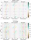 |
Fig. 6. Dynamic spectra of StKM 1-1262 and V374 Peg. The Stokes I profiles are phase-folded according to Eq. (1) and stacked vertically. From left, the panels show the observed, reconstructed and residual profiles. The colour bar indicates the flux values of Stokes I LSD profiles. In the observed and reconstructed panels, the Stokes I are median subtracted, hence positive and negative values of the colour bar indicate dark and bright features, respectively. The median subtraction removes stationary bumps, making them more evident in the residuals panel. The vertical solid line locates the radial velocity of the stars (−3.9 km s−1 for StKM 1-1262 and −5.0 km s−1 for V374 Peg), and the two dashed lines are located at the extremes of the intervals for the computation of Bℓ and ZDI (see Sect. 4 and Sect. 5). |
Our reconstructed brightness map of V374 Peg is illustrated in Fig. 7 and is consistent with the dynamic spectra. We note two dark regions around latitudes 50–60° with roughly 20% less intensity than the quiet photosphere, and three bright regions at similar latitudes with up to 40% larger intensity. Although it is not possible to compare this Doppler map with those of Morin et al. (2008a) exactly, because our model accounts for both dark and bright regions, there is general agreement in terms of the multitude of inhomogeneities and complexity of the surface on V374 Peg. The fact that the brightness maps of V374 Peg are consistent, despite being about 14 yr apart, is also consistent with the analysis of photometric light curves of Vida et al. (2016), which suggests a spot configuration that is stable over about 16 yr. In the case of V374 Peg, the comparison between the brightness map and the time series of total magnetic flux and effective temperature is less straightforward than StKM 1-1262, due to the lack of a clear rotational modulation of ⟨BI⟩ and Teff.
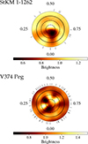 |
Fig. 7. Reconstructed brightness maps of StKM 1-1262 and V374 Peg. The colour bar indicates the brightness relative to the quiet photosphere, which is equal to 1.0. |
7. Discussion and conclusions
We have analysed SPIRou spectropolarimetric time series observations in circular polarisation mode of two stars, StKM 1-1262 and V374 Peg. Our aim is to provide robust and updated constraints on the magnetic field of the two stars, which is fundamental to understanding the mechanisms driving their detected radio emission. For StKM 1-1262, the detected radio emission has identical frequency and polarisation properties as fundamental plasma emission from a Solar Type II burst, and probably represents one of the few pieces of evidence of an extrasolar type-II burst (Tasse et al. 2021; Callingham et al. 2025). This detection suggests that CMEs can occur for stars whose fields are substantially stronger than the Sun’s (Alvarado-Gómez et al. 2018; Strickert et al. 2024). The magnetic field characterisation of StKM 1-1262 performed in this work has been used in Callingham et al. (2025) to support such conclusions.
From the unpolarised spectra, we modelled Zeeman broadening and intensification, constraining the total unsigned magnetic field ⟨BI⟩ to be 3.53 ± 0.06 kG for StKM 1-1262 and 5.46 ± 0.09 kG for V374 Peg. In terms of mass and rotation period, StKM 1-1262 is close to the binary system YY Gem, whose magnetic field characterisation was carried out by Kochukhov & Shulyak (2019). The authors measured a total magnetic field of 3.2–3.4 kG for the two stars in the binary, which is compatible with our value for StKM 1-1262. Our results are also similar to the early-M dwarf OT Ser, with a total unsigned magnetic field of 3.2 kG (Shulyak et al. 2019). For V374 Peg, our measurement is compatible with the estimate of 4.4 ± 1.0 kG by Shulyak et al. (2019) within uncertainties, and it is also consistent with stars in the vicinity of V374 Peg in terms of mass and rotation period, such as EQ Peg B (4.2 ± 1.0 kG; Shulyak et al. 2017).
We used the spectral fitting procedure to derive the values of the surface temperature Teff and ⟨BI⟩ simultaneously. We found a strong anti-correlation between total magnetic flux and effective temperature for StKM 1-1262, which is in agreement with the tight connection between the stellar surface temperature variations and the small-scale magnetic field, as already pointed out in Artigau et al. (2024) and Cristofari et al. (2025). For V374 Peg, we only obtained a moderate anti-correlation, which is most likely due to a combination of factors such as the low S/N of the observations; the larger veqsin(i) (hence rotational broadening); the low contrast between spots and quiet photosphere (of about 300 K); and potentially a more dense and homogeneous distribution of surface features than StKM 1-1262. The combined action of several surface spots, distributed homogeneously, could also explain the lack of a clear rotational modulation of Teff and ⟨BI⟩ for V374 Peg. This would be consistent with the fact that V374 Peg falls into the supersaturated regime of the activity-rotation relation (Wright et al. 2011), for which coronal X-ray emission decreases below the saturation level of LX/Lbol ∼ 10−3 with increasing rotation (e.g. Prosser et al. 1996). In fact, although V374 Peg is expected to be more active than StKM 1-1262, its X-ray emission is LX = 2.75 × 1028 erg/s (Delfosse et al. 1998), which is about one order of magnitude lower than that of StKM 1-1262 (LX = 2.20 × 1029 erg/s Agüeros et al. 2009). In this scenario, V374 Peg’s surface would be completely covered with active regions, in contrast to StKM 1-1262.
From the circularly polarised spectra, we first measured the longitudinal field. We found an average of −67 G for StKM 1-1262 and 351 G for V374 Peg, consistently showing a difference in magnetic activity level between the two stars. We then reconstructed the large-scale magnetic field by means of ZDI, and the results are contextualised in Fig. 8. We obtained predominantly poloidal-dipolar configurations with moderate axisymmetry for StKM 1-1262 and high axisymmetry for V374 Peg. The average magnetic field is 300 G and 800 G for the two stars. The ratio ⟨|BV|⟩/⟨BI⟩ between the magnetic field strength as recovered by circularly polarised (that is, ZDI) and unpolarised (that is, Zeeman broadening modelling) light is 8.5% for StKM 1-1262 and 15% for V374 Peg. Values of up to 10% are typical for partly convective M dwarfs (Reiners & Basri 2009; Morin et al. 2010; Kochukhov 2021), and up to 20% for fully convective M dwarfs, depending on the large-scale field geometry (see e.g. Kochukhov 2021). Therefore, both our findings are within expectations.
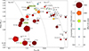 |
Fig. 8. Properties of the magnetic topologies for cool, main-sequence stars obtained via ZDI. The locations of StKM 1-1262 and V374 Peg are highlighted. The y- and x-axes represent the mass and rotation period of the star. Gray curves illustrate different Rossby numbers (Ro = 0.01, 0.1 and 1.0), and are obtained using the empirical relations of Wright et al. (2018). The Rossby number is the ratio between the rotation period of a star and the convective turnover time. The symbol size, colour, and shape encodes the ZDI average field strength, poloidal/toroidal energy fraction, and axisymmetry (see Petit et al. 2008; Morgenthaler et al. 2012; Fares et al. 2013; Boro Saikia et al. 2015; do Nascimento et al. 2016; Boro Saikia et al. 2016; Hussain et al. 2016; Alvarado-Gómez et al. 2015; Folsom et al. 2016, 2018; Kochukhov & Shulyak 2019; Folsom et al. 2020; Klein et al. 2021; Willamo et al. 2022; Martioli et al. 2022; Bellotti et al. 2023a; Lehmann et al. 2024, for the data used). For stars with multiple reconstructions, the data represent the most recent ZDI maps. |
Our ZDI reconstruction of StKM 1-1262 is, in general, in agreement with stars with similar properties, such as YY Gem (Kochukhov & Shulyak 2019). The situation is similar for V374 Peg, since Morin et al. (2008a) also reconstructed a largely poloidal-dipolar field with a high degree of axisymmetry. This suggests that the large-scale magnetic field of V374 Peg is stable over time, but the approximately 10-year gap between observations prevents us from being conclusive. Additional observations conducted annually will provide a definitive answer.
We also reconstructed the brightness map of both stars. For StKM 1-1262, we found the surface to be characterised by a dark spot lying approximately at rotational phase 0.0 (see Fig. 7). The structure of the brightness map is corroborated by the time series of ⟨BI⟩ and Teff, since their rotational modulation correlates with the presence of such a starspot. For V374 Peg, we reconstructed a more complex map, with multiple dark and bright regions, which is in overall agreement with previous reconstructions (Morin et al. 2008a), and the view that this star has a more homogeneous spot distribution. In this case, we did not observe a clear rotational modulation of ⟨BI⟩ or Teff, so connecting them to the Doppler map is less straightforward. From our analysis of the ⟨BI⟩-Teff anti-correlation, we obtained spot coverages of 25% and 48% for StKM 1-1262 and V374 Peg, which are higher than the mean spot coverage reconstructed via Doppler imaging of 9% and 17%, respectively. This discrepancy could be due to the fact that the temperature variations studied in Sect. 3 may be the result of large spots as well as several small ones, making the empirical relation in Eq. (2) more sensitive to different spatial scales than Doppler imaging. In fact, the spatial resolution attainable by Doppler imaging, which is further deteriorated by S/N considerations, is mostly limited to big spots or small spots clustered together.
Finally, the LoTTS survey has detected several low-mass stars with radio observations, regardless of the magnetic activity level of the star (Callingham et al. 2021). Shedding more light on the physical mechanism driving the radio emission, whether planet- or plasma-induced, for instance, requires a robust constraint on the magnetic field. Therefore, spectropolarimetric observations of these low-mass stars are required to fully understand their magnetism and plasma environment.
The code is available at https://github.com/folsomcp/LSDpy
http://vald.astro.uu.se/ using the Montpellier mirror to request locally MARCS model atmospheres.
Acknowledgments
We would like to thank Prof. B. Pope for the contribution to the SPIRou observing proposal of StKM 1-1262 and the comments for this manuscript. This publication is part of the project “Exo-space weather and contemporaneous signatures of star-planet interactions” (with project number OCENW.M.22.215 of the research programme “Open Competition Domain Science- M”), which is financed by the Dutch Research Council (NWO). PC and AAV acknowledge funding from the European Research Council (ERC) under the European Union’s Horizon 2020 research and innovation programme (grant agreement No 817540, ASTROFLOW). JRC acknowledges funding from the European Union via the European Research Council (ERC) grant Epaphus (project number 101166008) AAV acknowledges funding from the Dutch Research Council (NWO), with project number VI.C.232.041 of the Talent Programme Vici. MMJ acknowledges support from STFC consolidated grant number ST/R000824/1. Based on observations obtained at the Canada-France-Hawaii Telescope (CFHT) which is operated by the National Research Council of Canada, the Institut National des Sciences de l’Univers of the Centre National de la Recherche Scientique of France, and the University of Hawaii. This work has made use of the VALD database, operated at Uppsala University, the Institute of Astronomy RAS in Moscow, and the University of Vienna; Astropy, 12 a community-developed core Python package for Astronomy (Astropy Collaboration 2013, 2018); NumPy (van der Walt et al. 2011); Matplotlib: Visualization with Python (Hunter 2007); SciPy (Virtanen et al. 2020) and PyAstronomy (Czesla et al. 2019).
References
- Agüeros, M. A., Anderson, S. F., Covey, K. R., et al. 2009, ApJS, 181, 444 [CrossRef] [Google Scholar]
- Airapetian, V. S., Glocer, A., Khazanov, G. V., et al. 2017, ApJ, 836, L3 [NASA ADS] [CrossRef] [Google Scholar]
- Airapetian, V. S., Barnes, R., Cohen, O., et al. 2020, Int. J. Astrobiol., 19, 136 [NASA ADS] [CrossRef] [Google Scholar]
- Alvarado-Gómez, J. D., Hussain, G. A. J., Grunhut, J., et al. 2015, A&A, 582, A38 [NASA ADS] [CrossRef] [EDP Sciences] [Google Scholar]
- Alvarado-Gómez, J. D., Drake, J. J., Cohen, O., Moschou, S. P., & Garraffo, C. 2018, ApJ, 862, 93 [Google Scholar]
- Alvarado-Gómez, J. D., Cohen, O., Drake, J. J., et al. 2022, ApJ, 928, 147 [CrossRef] [Google Scholar]
- Artigau, É., Cadieux, C., Cook, N. J., et al. 2024, AJ, 168, 252 [Google Scholar]
- Astropy Collaboration (Robitaille, T. P., et al.) 2013, A&A, 558, A33 [NASA ADS] [CrossRef] [EDP Sciences] [Google Scholar]
- Astropy Collaboration (Price-Whelan, A. M., et al.) 2018, AJ, 156, 123 [Google Scholar]
- Bellotti, S., Fares, R., Vidotto, A. A., et al. 2023a, A&A, 676, A139 [NASA ADS] [CrossRef] [EDP Sciences] [Google Scholar]
- Bellotti, S., Morin, J., Lehmann, L. T., et al. 2023b, A&A, 676, A56 [NASA ADS] [CrossRef] [EDP Sciences] [Google Scholar]
- Bellotti, S., Morin, J., Lehmann, L. T., et al. 2024, A&A, 686, A66 [NASA ADS] [CrossRef] [EDP Sciences] [Google Scholar]
- Berdyugina, S. V. 2005, Liv. Rev. Sol. Phys., 2, 8 [Google Scholar]
- Boro Saikia, S., Jeffers, S. V., Petit, P., et al. 2015, A&A, 573, A17 [NASA ADS] [CrossRef] [EDP Sciences] [Google Scholar]
- Boro Saikia, S., Jeffers, S. V., Morin, J., et al. 2016, A&A, 594, A29 [NASA ADS] [CrossRef] [EDP Sciences] [Google Scholar]
- Callingham, J. R., Vedantham, H. K., Shimwell, T. W., et al. 2021, Nat. Astron., 5, 1233 [NASA ADS] [CrossRef] [Google Scholar]
- Callingham, J. R., Pope, B. J. S., Kavanagh, R. D., et al. 2024, Nat. Astron., 8, 1359 [NASA ADS] [CrossRef] [Google Scholar]
- Callingham, J. R., Tasse, C., & Keers, R. 2025, Nature, accepted [Google Scholar]
- Cane, H. V., Erickson, W. C., & Prestage, N. P. 2002, J. Geophys. Res. (Space Phys.), 107, 1315 [Google Scholar]
- Carolan, S., Vidotto, A. A., Loesch, C., & Coogan, P. 2019, MNRAS, 489, 5784 [NASA ADS] [CrossRef] [Google Scholar]
- Cherenkov, A., Bisikalo, D., Fossati, L., & Möstl, C. 2017, ApJ, 846, 31 [Google Scholar]
- Childs, A. C., Martin, R. G., & Livio, M. 2022, ApJ, 937, L41 [Google Scholar]
- Claret, A., & Bloemen, S. 2011, A&A, 529, A75 [NASA ADS] [CrossRef] [EDP Sciences] [Google Scholar]
- Cockell, C. S., Bush, T., Bryce, C., et al. 2016, Astrobiology, 16, 89 [NASA ADS] [CrossRef] [Google Scholar]
- Colman, I. L., Angus, R., David, T., et al. 2024, AJ, 167, 189 [Google Scholar]
- Cook, N. J., Artigau, É., Doyon, R., et al. 2022, PASP, 134, 114509 [NASA ADS] [CrossRef] [Google Scholar]
- Cotton, D. V., Evensberget, D., Marsden, S. C., et al. 2019, MNRAS, 483, 1574 [NASA ADS] [CrossRef] [Google Scholar]
- Cristofari, P. I., Donati, J. F., Masseron, T., et al. 2022, MNRAS, 511, 1893 [NASA ADS] [CrossRef] [Google Scholar]
- Cristofari, P. I., Donati, J.-F., Folsom, C. P., et al. 2023a, MNRAS, 522, 1342 [NASA ADS] [CrossRef] [Google Scholar]
- Cristofari, P. I., Donati, J. F., Moutou, C., et al. 2023b, MNRAS, 526, 5648 [NASA ADS] [CrossRef] [Google Scholar]
- Cristofari, P. I., Donati, J.-F., Bellotti, S., et al. 2025, A&A, 702, A111 [NASA ADS] [CrossRef] [EDP Sciences] [Google Scholar]
- Crosley, M. K., & Osten, R. A. 2018, ApJ, 862, 113 [NASA ADS] [CrossRef] [Google Scholar]
- Crosley, M. K., Osten, R. A., Broderick, J. W., et al. 2016, ApJ, 830, 24 [NASA ADS] [CrossRef] [Google Scholar]
- Cuntz, M. 2015, ApJ, 798, 101 [Google Scholar]
- Cuntz, M., & Wang, Z. 2020, Astron. Nachr., 341, 402 [Google Scholar]
- Cutri, R. M., Skrutskie, M. F., van Dyk, S., et al. 2003, VizieR Online Data Catalog, II/246 [Google Scholar]
- Czesla, S., Schröter, S., Schneider, C. P., et al. 2019, PyA: Python astronomy-related packages [Google Scholar]
- del Toro Iniesta, J. C. 2003, Introduction to Spectropolarimetry (Cambridge, UK: Cambridge University Press) [Google Scholar]
- Delfosse, X., Forveille, T., Perrier, C., & Mayor, M. 1998, A&A, 331, 581 [NASA ADS] [Google Scholar]
- Deutsch, A. J. 1957, AJ, 62, 139 [Google Scholar]
- do Nascimento, J. D. J., Vidotto, A. A., Petit, P., et al. 2016, ApJ, 820, L15 [NASA ADS] [CrossRef] [Google Scholar]
- Donati, J. F., & Brown, S. F. 1997, A&A, 326, 1135 [Google Scholar]
- Donati, J. F., Semel, M., Carter, B. D., Rees, D. E., & Collier Cameron, A. 1997, MNRAS, 291, 658 [Google Scholar]
- Donati, J. F., Morin, J., Petit, P., et al. 2008, MNRAS, 390, 545 [Google Scholar]
- Donati, J. F., Kouach, D., Moutou, C., et al. 2020, MNRAS, 498, 5684 [Google Scholar]
- Donati, J. F., Cristofari, P. I., Finociety, B., et al. 2023, MNRAS, 525, 455 [NASA ADS] [CrossRef] [Google Scholar]
- Donati, J.-F., Cristofari, P. I., Klein, B., Finociety, B., & Moutou, C. 2025, A&A, 700, A122 [NASA ADS] [CrossRef] [EDP Sciences] [Google Scholar]
- Driscoll, P., & Bercovici, D. 2013, Icarus, 226, 1447 [NASA ADS] [CrossRef] [Google Scholar]
- Dulk, G. A., Steinberg, J. L., Lecacheux, A., Hoang, S., & MacDowall, R. J. 1985, A&A, 150, L28 [NASA ADS] [Google Scholar]
- Elekes, F., & Saur, J. 2023, A&A, 671, A133 [NASA ADS] [CrossRef] [EDP Sciences] [Google Scholar]
- Erba, C., Folsom, C. P., David-Uraz, A., et al. 2024, ApJ, 977, 84 [NASA ADS] [CrossRef] [Google Scholar]
- Fares, R., Moutou, C., Donati, J. F., et al. 2013, MNRAS, 435, 1451 [NASA ADS] [CrossRef] [Google Scholar]
- Folsom, C. P., Petit, P., Bouvier, J., et al. 2016, MNRAS, 457, 580 [Google Scholar]
- Folsom, C. P., Bouvier, J., Petit, P., et al. 2018, MNRAS, 474, 4956 [NASA ADS] [CrossRef] [Google Scholar]
- Folsom, C. P., Fionnagáin, D. Ó, Fossati, L., et al. 2020, A&A, 633, A48 [NASA ADS] [CrossRef] [EDP Sciences] [Google Scholar]
- Folsom, C. P., Erba, C., Petit, V., et al. 2025, J. Open Source Software, 10, 7891 [Google Scholar]
- Gaia Collaboration 2020, VizieR Online Data Catalog: Gaia EDR3 (Gaia Collaboration, 2020), VizieR On-line Data Catalog: I/350. Originally published. In: 2021A&A..649A..1G; doi:10.5270/esa-1ug [Google Scholar]
- Gopalswamy, N., Yashiro, S., Akiyama, S., et al. 2008, Ann. Geophys., 26, 3033 [CrossRef] [Google Scholar]
- Gustafsson, B., Edvardsson, B., Eriksson, K., et al. 2008, A&A, 486, 951 [NASA ADS] [CrossRef] [EDP Sciences] [Google Scholar]
- Hallinan, G., Doyle, G., Antonova, A., et al. 2009, in 15th Cambridge Workshop on Cool Stars, Stellar Systems, and the Sun, (AIP), AIP Conf. Ser., 1094, 146 [Google Scholar]
- Hébrard, É. M., Donati, J. F., Delfosse, X., et al. 2016, MNRAS, 461, 1465 [CrossRef] [Google Scholar]
- Hirayama, T., & Moriyama, F. 1979, Sol. Phys., 63, 251 [Google Scholar]
- Hunter, J. D. 2007, Comput. Sci. Eng., 9, 90 [NASA ADS] [CrossRef] [Google Scholar]
- Hussain, G. A. J., Collier Cameron, A., Jardine, M. M., et al. 2009, MNRAS, 398, 189 [Google Scholar]
- Hussain, G. A. J., Alvarado-Gómez, J. D., Grunhut, J., et al. 2016, A&A, 585, A77 [NASA ADS] [CrossRef] [EDP Sciences] [Google Scholar]
- Jaime, L. G., Aguilar, L., & Pichardo, B. 2014, MNRAS, 443, 260 [Google Scholar]
- Kasting, J. F., Whitmire, D. P., & Reynolds, R. T. 1993, Icarus, 101, 108 [Google Scholar]
- Kavanagh, R. D., Vidotto, A. A., Fionnagáin, D. Ó., et al. 2019, MNRAS, 485, 4529 [NASA ADS] [CrossRef] [Google Scholar]
- Kavanagh, R. D., Vidotto, A. A., Klein, B., et al. 2021, MNRAS, 504, 1511 [Google Scholar]
- Kavanagh, R. D., Vidotto, A. A., Vedantham, H. K., et al. 2022, MNRAS, 514, 675 [CrossRef] [Google Scholar]
- Kervella, P., Arenou, F., & Thévenin, F. 2022, A&A, 657, A7 [NASA ADS] [CrossRef] [EDP Sciences] [Google Scholar]
- Khodachenko, M. L., Ribas, I., Lammer, H., et al. 2007, Astrobiology, 7, 167 [CrossRef] [Google Scholar]
- Klein, B., Donati, J.-F., Moutou, C., et al. 2021, MNRAS, 502, 188 [Google Scholar]
- Kochukhov, O. 2021, A&A, 29, 1 [Google Scholar]
- Kochukhov, O., & Lavail, A. 2017, ApJ, 835, L4 [Google Scholar]
- Kochukhov, O., & Shulyak, D. 2019, ApJ, 873, 69 [Google Scholar]
- Kochukhov, O., Makaganiuk, V., & Piskunov, N. 2010, A&A, 524, A5 [NASA ADS] [CrossRef] [EDP Sciences] [Google Scholar]
- Kopparapu, R. K. 2013, ApJ, 767, L8 [Google Scholar]
- Korhonen, H., Vida, K., Husarik, M., et al. 2010, Astron. Nachr., 331, 772 [Google Scholar]
- Lammer, H. 2013, Origin and Evolution of Planetary Atmospheres [Google Scholar]
- Lammer, H., Selsis, F., Ribas, I., et al. 2003, ApJl, 598, L121 [Google Scholar]
- Lammer, H., Lichtenegger, H. I. M., Kulikov, Y. N., et al. 2007, Astrobiology, 7, 185 [NASA ADS] [CrossRef] [Google Scholar]
- Landi Degl’Innocenti, E., & Landolfi, M. 2004, Polarization in Spectral Lines, 307 (Dordrecht: Kluwer Academic Publishers) [Google Scholar]
- Landstreet, J. D. 1988, ApJ, 326, 967 [Google Scholar]
- Lavail, A., Kochukhov, O., & Wade, G. A. 2018, MNRAS, 479, 4836 [NASA ADS] [CrossRef] [Google Scholar]
- Lazio, T., Joseph, W., Farrell, W. M., Dietrick, J., et al. 2004, ApJ, 612, 511 [NASA ADS] [CrossRef] [Google Scholar]
- Lehmann, L. T., & Donati, J. F. 2022, MNRAS, 514, 2333 [CrossRef] [Google Scholar]
- Lehmann, L. T., Donati, J. F., Fouqué, P., et al. 2024, MNRAS, 527, 4330 [Google Scholar]
- Lenardic, A., Jellinek, A. M., Foley, B., O’Neill, C., & Moore, W. B. 2016, J. Geophys. Res. (Planets), 121, 1831 [Google Scholar]
- Llama, J., Jardine, M. M., Wood, K., Hallinan, G., & Morin, J. 2018, ApJ, 854, 7 [Google Scholar]
- Lynch, C. R., Murphy, T., Lenc, E., & Kaplan, D. L. 2018, MNRAS, 478, 1763 [Google Scholar]
- Majumdar, S., Patel, R., Pant, V., & Banerjee, D. 2021, ApJ, 919, 115 [NASA ADS] [CrossRef] [Google Scholar]
- Marques, M. S., Zarka, P., Echer, E., et al. 2017, A&A, 604, A17 [NASA ADS] [CrossRef] [EDP Sciences] [Google Scholar]
- Martioli, E., Hébrard, G., Fouqué, P., et al. 2022, A&A, 660, A86 [NASA ADS] [CrossRef] [EDP Sciences] [Google Scholar]
- Matthews, L. D. 2019, PASP, 131, 016001 [NASA ADS] [CrossRef] [Google Scholar]
- McLean, M., Berger, E., & Reiners, A. 2012, ApJ, 746, 23 [Google Scholar]
- Morgenthaler, A., Petit, P., Saar, S., et al. 2012, A&A, 540, A138 [NASA ADS] [CrossRef] [EDP Sciences] [Google Scholar]
- Morin, J., Donati, J. F., Forveille, T., et al. 2008a, MNRAS, 384, 77 [CrossRef] [Google Scholar]
- Morin, J., Donati, J. F., Petit, P., et al. 2008b, MNRAS, 390, 567 [Google Scholar]
- Morin, J., Donati, J. F., Petit, P., et al. 2010, MNRAS, 407, 2269 [Google Scholar]
- Nichols, J. D., Burleigh, M. R., Casewell, S. L., et al. 2012, ApJ, 760, 59 [Google Scholar]
- Nindos, A., Aurass, H., Klein, K. L., & Trottet, G. 2008, Sol. Phys., 253, 3 [NASA ADS] [CrossRef] [Google Scholar]
- Osten, R. A., & Wolk, S. J. 2017, in Living Around Active Stars, eds. D. Nandy, A. Valio, & P. Petit, IAU Symp., 328, 243 [Google Scholar]
- Owen, J. E., & Jackson, A. P. 2012, MNRAS, 425, 2931 [Google Scholar]
- Peña-Moñino, L., Pérez-Torres, M., Varela, J., & Zarka, P. 2024, A&A, 688, A138 [NASA ADS] [CrossRef] [EDP Sciences] [Google Scholar]
- Penz, T., & Micela, G. 2008, A&A, 479, 579 [NASA ADS] [CrossRef] [EDP Sciences] [Google Scholar]
- Pérez-Torres, M., Gómez, J. F., Ortiz, J. L., et al. 2021, A&A, 645, A77 [NASA ADS] [CrossRef] [EDP Sciences] [Google Scholar]
- Petit, P., Donati, J. F., & Collier Cameron, A. 2002, MNRAS, 334, 374 [NASA ADS] [CrossRef] [Google Scholar]
- Petit, P., Donati, J. F., Aurière, M., et al. 2005, MNRAS, 361, 837 [Google Scholar]
- Petit, P., Dintrans, B., Solanki, S. K., et al. 2008, MNRAS, 388, 80 [NASA ADS] [CrossRef] [Google Scholar]
- Pineda, J. S., Hallinan, G., & Kao, M. M. 2017, ApJ, 846, 75 [Google Scholar]
- Plez, B. 2012, Turbospectrum: Code for spectral synthesis, Astrophysics Source Code Library [record ascl:1205.004] [Google Scholar]
- Pope, B. J. S., Callingham, J. R., Feinstein, A. D., et al. 2021, ApJ, 919, L10 [NASA ADS] [CrossRef] [Google Scholar]
- Prosser, C. F., Randich, S., Stauffer, J. R., Schmitt, J. H. M. M., & Simon, T. 1996, AJ, 112, 1570 [Google Scholar]
- Rees, D. E., & Semel, M. D. 1979, A&A, 74, 1 [NASA ADS] [Google Scholar]
- Reiners, A., & Basri, G. 2009, A&A, 496, 787 [NASA ADS] [CrossRef] [EDP Sciences] [Google Scholar]
- Rice, J. B., Wehlau, W. H., & Khokhlova, V. L. 1989, A&A, 208, 179 [NASA ADS] [Google Scholar]
- Ricker, G. R., Winn, J. N., Vanderspek, R., et al. 2014, J. Astron. Telesc. Instrum. Syst., 1, 014003 [Google Scholar]
- Rosén, L., & Kochukhov, O. 2012, A&A, 548, A8 [NASA ADS] [CrossRef] [EDP Sciences] [Google Scholar]
- Rugheimer, S., Kaltenegger, L., Segura, A., Linsky, J., & Mohanty, S. 2015, ApJ, 809, 57 [Google Scholar]
- Ryabchikova, T., Piskunov, N., Kurucz, R. L., et al. 2015, Phys. Scr., 90, 054005 [Google Scholar]
- Seales, J., & Lenardic, A. 2021, arXiv e-prints [arXiv:2106.14852] [Google Scholar]
- Semel, M. 1989, A&A, 225, 456 [NASA ADS] [Google Scholar]
- Shimwell, T. W., Röttgering, H. J. A., Best, P. N., et al. 2017, A&A, 598, A104 [NASA ADS] [CrossRef] [EDP Sciences] [Google Scholar]
- Shimwell, T. W., Hardcastle, M. J., Tasse, C., et al. 2022, A&A, 659, A1 [NASA ADS] [CrossRef] [EDP Sciences] [Google Scholar]
- Shulyak, D., Reiners, A., Engeln, A., et al. 2017, Nat. Astron., 1, 0184 [NASA ADS] [CrossRef] [Google Scholar]
- Shulyak, D., Reiners, A., Nagel, E., et al. 2019, A&A, 626, A86 [NASA ADS] [CrossRef] [EDP Sciences] [Google Scholar]
- Skilling, J., & Bryan, R. K. 1984, MNRAS, 211, 111 [NASA ADS] [CrossRef] [Google Scholar]
- Strickert, K. M., Evensberget, D., & Vidotto, A. A. 2024, MNRAS, 533, 1156 [Google Scholar]
- Tasse, C., Shimwell, T., Hardcastle, M. J., et al. 2021, A&A, 648, A1 [EDP Sciences] [Google Scholar]
- Treumann, R. A. 2006, A&A Rev., 13, 229 [NASA ADS] [CrossRef] [Google Scholar]
- Turner, J. D., Zarka, P., Grießmeier, J.-M., et al. 2021, A&A, 645, A59 [NASA ADS] [CrossRef] [EDP Sciences] [Google Scholar]
- Turnpenney, S., Nichols, J. D., Wynn, G. A., & Burleigh, M. R. 2018, ApJ, 854, 72 [Google Scholar]
- van der Walt, S., Colbert, S. C., & Varoquaux, G. 2011, Comput. Sci. Eng., 13, 22 [Google Scholar]
- Van Looveren, G., Güdel, M., Boro Saikia, S., & Kislyakova, K. 2024, A&A, 683, A153 [Google Scholar]
- Vedantham, H. K., Callingham, J. R., Shimwell, T. W., et al. 2020, Nat. Astron., 4, 577 [Google Scholar]
- Vida, K., Kriskovics, L., Oláh, K., et al. 2016, A&A, 590, A11 [NASA ADS] [CrossRef] [EDP Sciences] [Google Scholar]
- Vidotto, A. A., Jardine, M., Opher, M., Donati, J. F., & Gombosi, T. I. 2011, MNRAS, 412, 351 [NASA ADS] [CrossRef] [Google Scholar]
- Vidotto, A. A., Jardine, M., Morin, J., et al. 2013, A&A, 557, A67 [NASA ADS] [CrossRef] [EDP Sciences] [Google Scholar]
- Vidotto, A. A., Jardine, M., Morin, J., et al. 2014, MNRAS, 438, 1162 [Google Scholar]
- Vidotto, A. A., Feeney, N., & Groh, J. H. 2019, MNRAS, 488, 633 [Google Scholar]
- Villadsen, J., & Hallinan, G. 2019, ApJ, 871, 214 [Google Scholar]
- Virtanen, P., Gommers, R., Burovski, E., et al. 2020, scipy/scipy: SciPy 1.5.3 [Google Scholar]
- Vogt, S. S., & Penrod, G. D. 1983, PASP, 95, 565 [NASA ADS] [CrossRef] [Google Scholar]
- Wade, G. A., Bagnulo, S., Kochukhov, O., et al. 2001, A&A, 374, 265 [NASA ADS] [CrossRef] [EDP Sciences] [Google Scholar]
- Webb, D. F., & Howard, T. A. 2012, Liv. Rev. Sol. Phys., 9, 3 [Google Scholar]
- Willamo, T., Lehtinen, J. J., Hackman, T., et al. 2022, A&A, 659, A71 [NASA ADS] [CrossRef] [EDP Sciences] [Google Scholar]
- Wright, N. J., Drake, J. J., Mamajek, E. E., & Henry, G. W. 2011, ApJ, 743, 48 [Google Scholar]
- Wright, N. J., Newton, E. R., Williams, P. K. G., Drake, J. J., & Yadav, R. K. 2018, MNRAS, 479, 2351 [Google Scholar]
- Wu, C. S., & Lee, L. C. 1979, ApJ, 230, 621 [Google Scholar]
- Yiu, T. W. H., Vedantham, H. K., Callingham, J. R., & Günther, M. N. 2024, A&A, 684, A3 [NASA ADS] [CrossRef] [EDP Sciences] [Google Scholar]
- Zarka, P. 1998, J. Geophys. Res., 103, 20159 [Google Scholar]
- Zarka, P. 2007, Planet. Space Sci., 55, 598 [Google Scholar]
Appendix A: Journal of observations
In this appendix we report the log of the observations for StKM 1-1262 and V374 Peg. The table includes the ⟨BI⟩, Teff, and longitudinal field measurements for the two stars.
Observations for StKM 1-1262.
Observations for V374 Peg with the same format as Table A.1.
Appendix B: Additional figures
In this appendix we provide additional figures related to the atmospheric characterisation of the two stars and the correlation analysis between the total unsigned magnetic field, the absolute value of the longitudinal magnetic field and the stellar surface temperature.
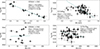 |
Fig. B.1. Correlation of the total unsigned field and longitudinal field with the stellar surface temperature. The left panels refer to StKM 1-1262 and the right ones to V374 Peg. The blue line indicates a linear fit, whose best-fit values are given in the each legend. We also include the Pearson correlation coefficient and the corresponding p-value. |
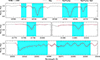 |
Fig. B.2. Example fit obtained on the template spectrum of StKM 1-1262. The cyan region shows regions on which the fit is performed. |
Appendix C: Simultaneous Stokes I and V modelling
In this appendix we present the Stokes I and V models for both StKM 1-1262 and V374 Peg. In Fig. C.1 and Fig. C.3, we show the Stokes V LSD profiles associated with the magnetic maps presented in Sect. 5. In Fig. C.2 and Fig. C.4, we show the Stokes I LSD profiles associated with the brightness maps presented in Sect. 6.
When performing ZDI, one typical assumption is that the brightness of the photosphere is homogeneous. Rosén & Kochukhov (2012) tested the reliability of ZDI reconstructions when high-contrast temperature spots are modelled simultaneously to the magnetic geometry in ideal conditions (i.e. high S/N, dense phase coverage, and large veq sin i). They found that the magnetic field strength is underestimated by 10-15% when temperature and magnetic spots are included, and by 30-60% when only magnetic spots are included. We decided to reconstruct the large-scale magnetic field of STKM 1-1262 and V374 Peg together with their brightness distribution, to double check the consistency of our results.
The maps are shown in Fig. C.5. The magnetic field topology of both stars does not change substantially. For StKM 1-1262, the poloidal energy fraction is increased by 3%, the dipolar by 6% (with consequent decrease in quadrupolar and octupolar fractions) and the axisymmetric component by 6%. The average field strength obtained when reconstructing Stokes I and V simultaneously is 15% lower. For V374 Peg, the configuration is more dipolar by 3% and axisymmetric by 6%, and the average field strength is 18% larger.
For the brightness map of StKM 1-1262, we observe a dark spot at a similar location than when reconstructing Stokes I alone, with a coverage slightly decreased to 8.5% and a lower contrast of 20% with respect to the quiet photosphere. In this case, the algorithm puts a bright feature at around phase 0.10 at a higher latitude with respect to the previous run with Stokes I alone, and shifts the phase of the already-present bright feature from 0.5 to 0.6. In the new reconstruction, the position of the bright features correlates with the location of the large-scale field component with negative polarity. For V374 Peg, the contrast of the brightness map is mostly dominated by a bright feature at around phase 0.4, which is the same pointing phase of the positive polarity of the large-scale magnetic field configuration. The code still reconstructs the same bright features at phases 0.2 and 0.6 and at a similar latitude, albeit with a smaller contrast with the quiet photosphere.
We note that magnetic effects can dominate the width of Stokes I LSD profiles rather than brightness inhomogeneities. Recent examples are the M dwarfs AU Mic and EV Lac described by Donati et al. (2023) and Donati et al. (2025), for which the authors find substantial differences in the width of Stokes I LSD profiles when computed with magnetically sensitive and insensitive lines separately. They assumed that the small-scale field locally scales up with the large-scale field, which allowed them to fit the Stokes I profiles width simultaneously with the Stokes V profiles, producing a large-scale magnetic field reconstruction consistent with the small-scale field. In our case, the change in width of the Sokes I LSD profiles is not large, likely due to rotational broadening being a dominant component, and its rotational modulation is not more or less evident when using magnetically insensitive and sensitive lines, respectively. Thus, we cannot apply the same methodology.
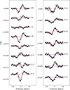 |
Fig. C.1. Time series of Stokes V LSD profiles and the ZDI models for StKM 1-1262. The observations are shown in black and the models in red. The numbers on the right indicate the rotational cycle computed from Eq. 1 using the first observation of an epoch as reference date. The horizontal line represents the zero point of the profiles, which are shifted vertically based on their rotational phase for visualisation purposes. |
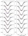 |
Fig. C.2. Time series of Stokes I LSD profiles and the DI models for StKM 1-1262. The format is the same as Fig C.1. The horizontal blue dashed line indicates the continuum level at 1.0, which is shifted vertically for visualisation purposes. |
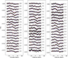 |
Fig. C.3. Time series of Stokes V LSD profiles and the ZDI models for V374 Peg. The format is the same as Fig. C.1. |
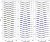 |
Fig. C.4. Time series of Stokes I LSD profiles and the DI models for V374 Peg. The format is the same as Fig. C.2. |
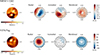 |
Fig. C.5. Simultaneous brightness and magnetic reconstruction. The format is the same as Fig. 7 for the brightness part and Fig. 5 for the magnetic part. |
All Tables
All Figures
|
Fig. 1. Distribution of magnetic flux on different magnetic components. The top panel refers to StKM 1-1262 and the bottom panel to V374 Peg. |
| In the text | |
|
Fig. 2. Total magnetic field measurements of StKM 1-1262 and V374 Peg as a function of rotational phase. The data points are colour-coded with the effective temperature obtained from spectral modelling (see Sect. 3). The rotational phases are computed according to Eq. (1), using the stellar rotation period listed in Table 1. |
| In the text | |
|
Fig. 3. Longitudinal magnetic field measurements of StKM 1-1262 and V374 Peg. The panels show Bℓ as a function of rotational phase for StKM 1-1262 and V374 Peg. The rotational phases are computed according to Eq. (1), using the rotational period listed in Table 1. |
| In the text | |
|
Fig. 4. Long-term measurements of V374 Peg’s longitudinal magnetic field. The leftmost epochs (coloured with light brown) represent the August 2005, August 2006, and September 2009 time series analysed by Morin et al. (2008a). The rightmost (dark brown) time series corresponds to the data analysed in this work. |
| In the text | |
|
Fig. 5. Reconstructed large-scale magnetic field maps in flattened polar view. StKM 1-1262 is shown in the top row and V374 Peg in the bottom row. From the left, the radial, azimuthal, and meridional components of the magnetic field vector are illustrated. Concentric circles represent different stellar latitudes: −30 °, +30 °, and +60 ° (dashed lines), as well as the equator (solid line). The radial ticks are located at the rotational phases when the observations were collected. The rotational phases are computed with Eq. (1), using the first observation of each individual epoch (see Table A.1). The colour bar indicates the polarity and strength (in G) of the magnetic field. |
| In the text | |
|
Fig. 6. Dynamic spectra of StKM 1-1262 and V374 Peg. The Stokes I profiles are phase-folded according to Eq. (1) and stacked vertically. From left, the panels show the observed, reconstructed and residual profiles. The colour bar indicates the flux values of Stokes I LSD profiles. In the observed and reconstructed panels, the Stokes I are median subtracted, hence positive and negative values of the colour bar indicate dark and bright features, respectively. The median subtraction removes stationary bumps, making them more evident in the residuals panel. The vertical solid line locates the radial velocity of the stars (−3.9 km s−1 for StKM 1-1262 and −5.0 km s−1 for V374 Peg), and the two dashed lines are located at the extremes of the intervals for the computation of Bℓ and ZDI (see Sect. 4 and Sect. 5). |
| In the text | |
|
Fig. 7. Reconstructed brightness maps of StKM 1-1262 and V374 Peg. The colour bar indicates the brightness relative to the quiet photosphere, which is equal to 1.0. |
| In the text | |
|
Fig. 8. Properties of the magnetic topologies for cool, main-sequence stars obtained via ZDI. The locations of StKM 1-1262 and V374 Peg are highlighted. The y- and x-axes represent the mass and rotation period of the star. Gray curves illustrate different Rossby numbers (Ro = 0.01, 0.1 and 1.0), and are obtained using the empirical relations of Wright et al. (2018). The Rossby number is the ratio between the rotation period of a star and the convective turnover time. The symbol size, colour, and shape encodes the ZDI average field strength, poloidal/toroidal energy fraction, and axisymmetry (see Petit et al. 2008; Morgenthaler et al. 2012; Fares et al. 2013; Boro Saikia et al. 2015; do Nascimento et al. 2016; Boro Saikia et al. 2016; Hussain et al. 2016; Alvarado-Gómez et al. 2015; Folsom et al. 2016, 2018; Kochukhov & Shulyak 2019; Folsom et al. 2020; Klein et al. 2021; Willamo et al. 2022; Martioli et al. 2022; Bellotti et al. 2023a; Lehmann et al. 2024, for the data used). For stars with multiple reconstructions, the data represent the most recent ZDI maps. |
| In the text | |
|
Fig. B.1. Correlation of the total unsigned field and longitudinal field with the stellar surface temperature. The left panels refer to StKM 1-1262 and the right ones to V374 Peg. The blue line indicates a linear fit, whose best-fit values are given in the each legend. We also include the Pearson correlation coefficient and the corresponding p-value. |
| In the text | |
|
Fig. B.2. Example fit obtained on the template spectrum of StKM 1-1262. The cyan region shows regions on which the fit is performed. |
| In the text | |
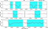 |
Fig. B.3. Same as Fig. B.2 but for V374 Peg. |
| In the text | |
|
Fig. C.1. Time series of Stokes V LSD profiles and the ZDI models for StKM 1-1262. The observations are shown in black and the models in red. The numbers on the right indicate the rotational cycle computed from Eq. 1 using the first observation of an epoch as reference date. The horizontal line represents the zero point of the profiles, which are shifted vertically based on their rotational phase for visualisation purposes. |
| In the text | |
|
Fig. C.2. Time series of Stokes I LSD profiles and the DI models for StKM 1-1262. The format is the same as Fig C.1. The horizontal blue dashed line indicates the continuum level at 1.0, which is shifted vertically for visualisation purposes. |
| In the text | |
|
Fig. C.3. Time series of Stokes V LSD profiles and the ZDI models for V374 Peg. The format is the same as Fig. C.1. |
| In the text | |
|
Fig. C.4. Time series of Stokes I LSD profiles and the DI models for V374 Peg. The format is the same as Fig. C.2. |
| In the text | |
|
Fig. C.5. Simultaneous brightness and magnetic reconstruction. The format is the same as Fig. 7 for the brightness part and Fig. 5 for the magnetic part. |
| In the text | |
Current usage metrics show cumulative count of Article Views (full-text article views including HTML views, PDF and ePub downloads, according to the available data) and Abstracts Views on Vision4Press platform.
Data correspond to usage on the plateform after 2015. The current usage metrics is available 48-96 hours after online publication and is updated daily on week days.
Initial download of the metrics may take a while.