© The Authors 2025

1 Introduction

In the last decade, three dense ring systems have been discovered around small bodies of the Solar System. Two rings have been observed around the Centaur object Chariklo (Braga-Ribas et al. 2014; Sicardy et al. 2018), one ring is known around the dwarf planet Haumea (Ortiz et al. 2017), and two rings have been detected around the trans-Neptunian object Quaoar (Morgado et al. 2023; Pereira et al. 2023). Meanwhile, dense and transient material that could be a ring in formation has been detected around the Centaur Chiron (Ortiz et al. 2023; Pereira et al. 2025).

The above-mentioned rings differ by a factor of five in terms of orbital radii and heliocentric distances (see the reviews by Sicardy et al. 2018 and Sicardy et al. 2024). Moreover, in the case of Quaoar, the rings are well beyond the classical Roche limit, which challenges the very concept of Roche’s zone. Another peculiarity of Quaoar’s main ring is that its optical depth significantly varies in longitude, recalling Neptune’s ring arc system (De Pater et al. 2018).

Meanwhile, these rings share common properties. They are all dense, in the sense that their optical depths range from about 1% to more than unity, implying that the particles suffer a few to tens of collisions per revolution. Thus, they must be considered as collisional disks, as opposed to tenuous dusty rings where particles move essentially independently of one another. Another common property of these rings is that they are strongly confined over radial distances ranging from a few kilometers to a few tens of kilometers, calling for an active confining mechanism. Finally, all these rings orbit close to a second-order resonance with the central body. More precisely, Chariklo’s, Haumea’s, and Quaoar’s main rings are close to the 1/3 resonance, meaning that a ring particle completes one revolution when the body completes three rotations, while Quaoar’s fainter ring orbit close the 5/7 resonance, where particles complete five revolutions during seven rotations of the body.

In this context, we have investigated the behavior of collisional rings around irregular bodies, with applications to Chariklo, Haumea, and Quaoar. Our results are presented in two papers. The current paper (“Paper I”) mainly deals with analytical to semi-analytical calculations, focusing on the dynamical structures of resonances of various orders around an irregular body. The second paper by Salo & Sicardy (2025) (“Paper II” hereafter) presents results obtained with N-body simulations of collisional rings perturbed by resonances, and is the numerical counterpart of this paper. These two papers are more detailed versions of previous works presented by Salo et al. (2021), Sicardy et al. (2021), Salo & Sicardy (2024), and Sicardy & Salo (2024), in which the dense mesh of resonances around irregular objects of the Solar System and the importance of the 1/3 SOR for confining rings were pointed out.

2 Resonances around an irregular body

We considered a test particle moving in the equatorial plane of a body of mass M. The universal gravitational constant is noted as G and time is noted as t, while r, r, and L denote the position vector, the radial distance to the body center of mass, and the true longitude of the particle, respectively. The Keplerian orbital elements of the particle are denoted as a, e, λ, ϖ (semimajor axis, orbital eccentricity, mean longitude, and longitude of pericenter, respectively), while n denotes the mean motion of the particle.

In addition to the spherical potential¹, −GM/r, created by the body, the axisymmetric terms of the potential (e.g., due to the body’s oblateness) force a secular apsidal precession rate, ${\dot{\varpi }}_{\sec }$, of the particle. Moreover, the non-axisymmetric terms create the spin–orbit resonances (SORs) considered in this paper. They may stem from a mass anomaly due to topographic features (mountains, craters, etc.), a “mascon” inside the body, a triaxial shape, or more complex shapes.

The pattern speed of the potential is equal to the spin rate, Ω_B, of the body. The orientation of the mass anomaly (or the major axis of the triaxial body) in inertial space is specified by its mean longitude, λ′ = Ω_Bt. The gravitational potential at r is then $$U\left(\mathbf{\text{r}}\right)={\displaystyle \sum _{m=-\infty }^{+\infty }{U}_m\left(r\right)\cos \left(m\theta \right)},$$(1)

where θ = L − λ′. The terms U_m(r) depend on the particular problem under consideration. The expression of U_m(r) for a mass anomaly is given in Appendix A, while its expression for a homogeneous triaxial ellipsoid is provided in Appendix B.

In Eq. (1), we have chosen to vary m from −∞ to +∞ rather than from 0 to +∞, implying that U_m(r) = U_−m(r). This choice is arbitrary and made to align with the symmetry in our resonance labeling, where m can be either positive or negative (see below).

Two types of resonances occur around the body. The corotation resonance is defined by $$n={\Omega }_{\text{B}},$$(2)

while the m/(m − j) SORs correspond to $$j\kappa =m\left(n-{\Omega }_{\text{B}}\right),$$(3)

where $\kappa =n-\dot{\varpi }$ is the epicyclic frequency of the particle. By convention, the integer j (called the order of the resonance hereafter) is always positive. In contrast, m can be positive (resp. negative) corresponding to inner (resp. outer ) resonances that occur inside (resp. outside) the corotation radius.

In this paper, first-order resonances (j = 1) are also referred to as Lindblad resonances. The nomenclature “m/(m − j) SOR” stems from the fact that Eq. (3) can be rewritten as $$\frac{n-\dot{\varpi }}{{\Omega }_{\text{B}}-\dot{\varpi }}=\frac{m}{m-j}\approx \frac{n}{{\Omega }_{\text{B}}},$$(4)

where the approximation is valid only if $\dot{\varpi }\ll n,{\Omega }_{\text{B}}$, which is usually the case in planetary problems. In galactic dynamics, this is not true anymore, so the notation “m/(m − j) resonance” becomes meaningless. Another notation – not to be confused with the one adopted here – is then used; for instance, “m : 1 Lindblad resonance” for the case j = 1 (see e.g., Pfenniger 1984).

The potential, U(r), can be expressed in terms of the Keplerian elements of the particle and Fourier-expanded under the form $$U\left(a,e,\lambda ,\varpi ,{\lambda }^{\prime }\right)={\displaystyle \sum _{m=-\infty }^{+\infty }{\displaystyle \sum _{j=0}^{+\infty }{\overline{U}}_{m,j}\left(\alpha \right)e^j\cos }\left({\psi }_{m,j}\right),}$$(5)

where $${\psi }_{m,j}=m{\lambda }^{\prime }-\left(m-j\right)\lambda -j\varpi$$(6)

and α = a/R_ref, where R_ref is a reference radius that gives the characteristic size of the object; for instance, its radius if it is a sphere. More complex expressions are obtained for a triaxial object (see Eq. (B.1)). In each term of the sum, we have kept only the lowest-order term in eccentricity; that is, e^j. The terms Ū_m,j(α)’s are given by $${\overline{U}}_{m,j}\left(\alpha \right)=2F_N\left[U_m\left(\alpha \right)\right],$$(7)

where the F_N are linear operators acting on U_m(α) that contain only multiplicative factors and derivatives with respect to a up to degree j. They are labeled by the index N, according to the nomenclature of Murray & Dermott (2000) or Ellis & Murray (2000) (see Sicardy (2020) for details and Appendix C for a summary). The operators’ F_N are listed in Table C.1 for first-and second-order SORs only, because higher-order resonances are not expected to have a significant effect on a collisional disk, as will be shown later. We point out that in the case of a mass anomaly and |m| = 1, the potential, U_m(α), contains an indirect term (Eq. (A.4)) that is automatically included to calculate Ū_m,j(α) from Eq. (7).

Caution must be taken with the factor two appearing in Eq. (7). It should be used only if the azimuthal number, m, appearing in Eq. (1) varies from −∞ to +∞, as it does here. If m varies 0 to +∞ in Eq. (1), as is the case in the literature for the potential of a satellite, then Eq. (7) must be replaced by Ū_m,j(α) = F_N [Um(α)].

We note that Eq. (7) can be used for any potential with the form of Eq. (1). It has the advantage of encapsulating in a single formula inner and outer resonances including possible indirect terms, or even retrograde resonances if n/Ω_B < 0.

3 Jacobi constant and phase portraits

Appendix D is a summary of how the classical Hamiltonians corresponding to SORs of any order, j, are obtained. It provides all the expressions that will be necessary from this section through Sect. 6. We first note that the phase portraits of the resonances are parameterized by the Jacobi constant, J. We hereafter use two equivalent forms of J. One is the dimensionless form, $$\Delta J=\frac{1}{2}\left[\frac{\Delta a}{a_0}+\left(\frac{m-j}{j}\right)e^2\right],$$(8)

where ∆a = a − a₀ and a₀ is the semimajor axis at an “exact” resonance, i.e., where the condition (3) is met. Thus, the condition ∆J = 0 can loosely be viewed as a definition of the center of the resonance. The Jacobi constant can also be expressed through the quantity $$\overline{a}=a_0\left(1+2\Delta J\right)=a+a_0\left(\frac{m-j}{j}\right)e^2,$$(9)

which has the dimension of a length. It is hereafter referred to as the “modified semimajor axis.” It corresponds to the semimajor axis of the circular orbit of a particle that has the constant of motion ∆J. The main advantage of using ā over a is that it is constant of motion time for a particle in the m/(m − j) resonance, once high-frequency terms have been averaged out. Meanwhile, since e is generally small, it also gives a good assessment of the particle’s semimajor axis.

For a given value of ∆J (or ā), a test particle evolves in a determined phase portrait, as is illustrated in Fig. 1. We distinguish two kinds of periodic orbits. The first-kind orbits correspond to fixed points near or at the origin of the phase portrait (e = 0), while the second-kind orbits correspond to fixed points with e ≠ 0.

In a collisional ring perturbed by a SOR, two opposite trends are at work. Collisions tend to damp eccentricities, and thus push the particles toward the origin of the phase portrait, which corresponds to a downward motion in the (ā, e) space. Conversely, the SORs tend to take the particles toward second-kind orbits, while maintaining constant ā, and thus correspond to an upward vertical motion in the (ā, e) space. We examine in the next two sections the dynamical stability of first-kind orbits and the locations of the second-kind orbits in the phase portraits.

4 Stability of first-kind orbits

To within a constant factor that is ignored, the Hamiltonian describing the m/(m − j) resonance (Eq. (D.1)) can be rewritten as $$\mathcal{H}=3\Delta J\left(\frac{m-j}{2j}\right)e^2-\frac{3}{2}{\left(\frac{m-j}{2j}\right)}^2{e}^2+ϵe^j\cos \left(j\varphi \right),$$(10)

where the resonant angle, ϕ, is² $$\varphi =\frac{{\psi }_{m,j}}{j}=\frac{m{\lambda }^{\prime }-\left(m-j\right)\lambda -j\varpi }{j}.$$(11)

The parameter ϵ quantifies the strength of the resonance. It depends on m and j and is defined by $$ϵ=\frac{{\overline{U}}_{m,j}\left(\alpha \right)}{a_0^2{n}_0^2}.$$(12)

See Appendices C and D for details.

Case j = 1. The Hamiltonian can be expressed in terms of the mixed variables X = e cos(ϕ) and Y = e sin(ϕ). At the origin of the phase portrait (X = Y = 0), Eq. (D.6) yields Ẋ = 0 and Ẏ = ϵ ≠ 0. Thus, for first-order resonances the origin of the phase portrait is never a fixed point. A particle placed on a circular orbit will always sees its orbital eccentricity initially increase (see Fig. 1).

For higher-order resonances (j ≥ 2), ℋ is on the order of at least two in eccentricity, i.e., it contains a homogeneous polynomial, P(X, Y), of at least degree two (Eq. (D.5)). Consequently, the origin of the phase portrait is always a fixed point. However, the nature of the this point (elliptic vs. hyperbolic) depends on j.

Case j = 2. To the lowest order in eccentricity, and from Eq. (10), we have near the origin $$\mathcal{H}\approx \left[\frac{3}{4}\left(m-2\right)\Delta J+ϵ\cos \left(2\varphi \right)\right]e^2.$$

Thus, in the finite interval of Jacobi constant $$-\frac{4}{3}\left|\frac{ϵ}{m-2}\right|<\Delta J<+\frac{4}{3}\left|\frac{ϵ}{m-2}\right|,$$(13)

the sign of ℋ changes in two directions as ϕ varies from 0 to 2π. The origin is then a fixed hyperbolic (unstable) point with two homoclinic trajectories in the directions defined by 3(m − 2)∆J/4 + ϵ cos(2ϕ) = 0. A particle launched on a circular orbit with those values of ∆J will have its orbital eccentricity increased in a first phase (Fig. 1).

Outside the interval given above, the origin of the phase portrait is a fixed elliptic (stable) point. A particle launched on a circular orbit will remain on this circular orbit.

Case j = 3. To the lowest orders in eccentricity, we again have near the origin $$\mathcal{H}\approx \frac{1}{2}\left(m-3\right)\Delta J{e}^2+ϵe^3\cos \left(3\varphi \right).$$

If ∆J ≠ 0, the second-order term dominates the expression of ℋ, so that the origin is an elliptic point. If ∆J = 0, ℋ is dominated by the third-order term. The Hamiltonian changes its sign in the three homoclinic directions defined by cos(3ϕ) = 0 (Fig. 1). However, and contrarily to the second-order resonances case, this happens only for an isolated value of ∆J.

Case j = 4. To the lowest orders in eccentricity, we have near the origin $$H\approx \frac{3}{8}\left(m-3\right)\Delta J{e}^2+\left[ϵ\cos \left(4\varphi \right)-\frac{3}{128}{\left(m-4\right)}^2\right]e^4.$$

If ∆J ≠ 0, the origin is an elliptic point. For ∆J = 0, the origin remains an elliptic point as long as e remains in the interval $$-\frac{3}{128}{\left(m-4\right)}^2<ϵ<+\frac{3}{128}{\left(m-4\right)}^2.$$(14)

In the opposite case, the origin is an hyperbolic point with four homoclinic directions. However, this requires |ϵ| to be quite large, a situation that is usually not encountered.

Case j ≥ 5. Near the origin, the Hamiltonian is now dominated either by isotropic terms of order two (∆J ≠ 0) or order four (∆J = 0) in eccentricity, so that the origin is always an elliptic point.

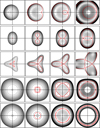Fig. 1 Representative phase portraits of resonances with orders j=1, 2, 3, 4, and 5, from top to bottom, respectively. Each phase portrait shows level curves of the Hamiltonians ℋ(X, Y) given in Eq. (D.5), where the mixed variables X and Y (Eq. (D.3)) define the eccentricity vector, e (Eq. (D.4)). The fixed elliptic points away from the origins correspond to maxima of ℋ(X, Y). For each resonance, four representative values of ∆J decreasing from left to right have been considered to illustrate the varying topologies of the phase portraits. The homoclinic trajectories are drawn in red. In all the plots, the value of the parameter ϵ appearing in Eq. (D.5) is taken as negative, as is the case for outer resonances. The topology of resonances with orders j > 5 are similar to the case j=5, except that there are j islands instead of five, with widths that decrease as j increases.

5 Second-kind orbits

The second-kind (or resonant) orbits are given by the fixed points of the phase portraits with e ≠ 0, as is shown in Fig. 1. At these points, ∂ℋ/∂ϕ = ∂ℋ/∂Θ = 0. In particular, ∂ℋ/∂Θ = 0 yields sin(jϕ) = 0, so that the fixed points lie in the directions defined by $${\phi }_k=\frac{k\pi }{j}\left(k=0,\dots ,2j-1\right),$$

in the phase portrait, where cos(jφ_k) = (−1)^k. We define the “φ_k axis” as the line that makes an angle, φ_k, with the X axis, so that the 0 axis is the X axis, the π/2 axis is the Y axis, and so on.

The equation ∂ℋ/∂ϕ = 0 then provides the modulus, e, of the eccentricity vector corresponding to the fixed points, i.e., $$e^2=\frac{2j}{m-j}\left[\Delta J+\frac{{\left(-1\right)}^k{j}^2ϵ}{3\left(m-j\right)}{e}^{j-2}\right]\left(k=0,\dots 2j-1\right).$$(15)

This equation can be projected onto the φ_k axis, yielding $$E^2=\left(\frac{2j}{m-j}\right)\Delta J+{\left(-1\right)}^kϵ\prime E^{j-2}\left(k=0,\dots ,2j-1\right),$$(16)

where E is an algebraic (positive or negative) quantity representing the eccentricity. In order to simplify the expressions obtained hereafter, we introduce a change of variable that reads $$ϵ\prime =\frac{2j^3}{3{\left(m-j\right)}^2}ϵ.$$(17)

For j = 1, it is sufficient to consider the case k = 0, corresponding to fixed points along the X axis. For j ≥ 2, it is enough to consider the cases k = 0 and k=1, as all the remaining cases, k = 2,…,2j − 1, are a mere repetition of Eq. (16), due to the invariance of the Hamiltonian under rotations of 2π/j radians.

Case j = 1. Equation 16 becomes $$X^3=\left(\frac{2\Delta J}{m-1}\right)X+ϵ\prime .$$(18)

This cubic equation can be solved in the manner described in Appendix E. In particular, Eq. (18) is identical to Eq. (E.1), taking $$\{\begin{array}{l}p=-\frac{2\Delta J}{m-1},\hfill \\ q=-ϵ\prime .\hfill \end{array}$$(19)

The discriminant of the cubic equation, Eq. (18), is $$\Delta =32{\left(\frac{\Delta J}{m-1}\right)}^3-27ϵ{\prime }^2.$$

For Δ < 0, there is one fixed point given by Eq. (E.3), and for Δ ≥ 0, there are three fixed points given by E.4. These solutions are plotted in panel a of Fig. 2.

Case j = 2. Eq. (16) reads $$E^2=\left(\frac{4\Delta J}{m-2}\right)+{\left(-1\right)}^kϵ\prime .$$(20)

For k = 0 (resp. k = 1), the fixed points are on the X axis (resp. Y axis). The solutions of the equation above are $$\begin{array}{c}{X}_{\text{f}}=\pm \sqrt{\left(\frac{4}{m-2}\right)\Delta J+ϵ\prime }\\ Y_{\text{f}}=\pm \sqrt{\left(\frac{4}{m-2}\right)\Delta J-ϵ\prime }\end{array}$$(21)

and are plotted in panel (b) of Fig. 2.

Case j = 3. Eq. (16) provides $$E^2=\left(\frac{6\Delta J}{m-3}\right)+{\left(-1\right)}^kϵ\prime E.$$(22)

The resulting solutions, $$E_{\text{f}}={\left(-1\right)}^k\left(\frac{ϵ\prime }{2}\right)\pm \sqrt{\left(\frac{6\Delta J}{m-3}\right)+\frac{ϵ{\prime }^2}{4}},$$(23)

are plotted in panel c Fig. 2. The case k = 0 corresponds to the fixed points along the X axis, while k = 1 corresponds to the fixed points along the π/3 axis.

Case j = 4. We now have $$E^2=\left(\frac{8\Delta J}{m-4}\right)+{\left(-1\right)}^kϵ\prime E^2,$$(24)

which yields $$E_{\text{f}}=\pm \sqrt{\left(\frac{8\Delta J}{m-4}\right)\left[\frac{1}{1-{\left(-1\right)}^kϵ\prime }\right]}$$(25)

(see panel d of Fig. 2). The case k = 0 corresponds to the fixed points along the X axis, while k = 1 corresponds to the fixed points along the π/4 axis.

Case j ≥ 5. A new regime appears beyond the order four. The term containing ϵ′ in Eq. (16) is of an order larger than two in E. Consequently, considering that both ϵ′ and E are small, we have $$E_{\text{f}}\approx \pm \sqrt{\left(\frac{2j}{m-j}\right)\Delta J},$$(26)

with a relative error of order ${ϵ}^{\prime }{E}_{\text{f}}^{j-4}$. These solutions are plotted in panel (e) of Fig. 2. The values of E_f are now independent of ϵ′. This means than the fixed points (excluding the origin) are distributed along a circle, with j elliptic points alternating with j hyperbolic points.

Eq. (26) has a straightforward interpretation. The expression of δJ (Eq. (8)) implies that the fixed point corresponds to a = a₀. This merely means that the corresponding orbits are then at exact resonance, as is expected. This is why the plot in panel (e) of Fig. 2 is undistinguishable from the unperturbed case (ϵ′ = 0).

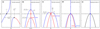Fig. 2 Fixed points given by Eq. (16) as a function of ΔJ for resonances of various orders. They are the solutions of Eqs. (18), (20), (22), (24), and (26). In all the plots, the values of ϵ′ are taken as negative, as is the case for outer resonances. The cubic root, ϵ′1/3, is then understood as the real root, i.e., ignoring the complex roots. The blue (resp. red) branches corresponding to stable elliptic (resp. unstable hyperbolic) points. Similarly, blue (resp. red) dots at the origin indicate a stable (resp. unstable) point. The units of all the plots are arbitrary. Panel a: first-order resonances. The positions of two particular points are specified: the solution corresponding to ΔJ = 0 and the pitchfork bifurcation point at the lower right. Panel b: second-order resonances. The parabolic branches are the solutions of Eq. (20). The positions of three particular points are specified. Panel c: third-order resonances. The parabolic branches are the solutions of Eq. (22). The positions of three particular points are specified. The origin of the phase portrait (Xf = Ef =0) is stable everywhere, except for the value ΔJ = 0 (red dot), where it is hyperbolic. Panel d: fourth-order resonances. The parabolic branches are the solutions of Eq. (24). The origin of the phase portrait (Xf = Ef =0) is stable everywhere, except for large values of ϵ (see Eq. (14)). Panel e: resonances of orders j ≥ 5. In this case, Xf = Ef (Eq. (26)), so that the stability of the points corresponding to each branch cannot be indicated on the plot; hence, the black color used here. This plot is now indistinguishable from the unperturbed case (ϵ′ = 0).

6 Behavior of the eccentricity near a resonance

The behavior of ring particles in a dense collisional disk at the vicinity of a resonance is complex due to the combination of various effects, including the differential precession rate, self-gravity, and viscous effects that lead to local angular momentum flux reversal. These issues are best tackled using the equations of hydrodynamic or N-body collisional simulations (see Paper II).

Meanwhile, it is instructive to estimate the maximum limit, e_max, of the orbital eccentricity of test particles initially on circular orbits, knowing that collisions will tend to damp eccentricities below this value. Sections 4 and 5 and Figs. 1 and 2 show that only three types of resonances yield unstable first-kind orbits: (i) first-order resonances, which force an eccentricity for any value of ΔJ; (ii) second-order resonances, which force an eccentricity only inside a finite interval of ΔJ (Eq. (13)); and (iii) third-order resonances, which force a nonzero eccentricity at the isolated value ΔJ = 0.

6.1 First-order resonances

We considered a particle that starts on a circular orbit with a Hamiltonian value of ℋ(0, 0) = ℋ₀. The particle then follows the level curve ℋ(X, Y) = ℋ₀. The eccentricity reaches its maximum value, e_max = |X_sup|, on the X axis, where X_sup is the nonzero solution of ℋ(X, 0) = ℋ₀, i.e., $$X^3-\left(\frac{4\Delta J}{m-1}\right)X-4ϵ\prime =0.$$(27)

Similar to what was done in Sect. 5, we identified Eq. (27) with the cubic equation, Eq. (E.1), taking $$\{\begin{array}{l}p=-\frac{4\Delta J}{m-1},\hfill \\ q=-4ϵ\prime ,\hfill \end{array}$$(28)

from which we obtained the discriminant $$\Delta =16\left[16{\left(\frac{\Delta J}{m-1}\right)}^3-27ϵ{\prime }^2\right].$$

In the case of δ < 0, the solution is, from Eq. (E.3), $$e_{\max }=\left|{\left(\frac{-q-\sqrt{-\Delta /27}}{2}\right)}^{1/3}+{\left(\frac{-q+\sqrt{-\Delta /27}}{2}\right)}^{1/3}\right|.$$(29)

If δ ≥ 0, there are three possible solutions given by Eq. (E.4). The one we are looking for is the one closest to the origin, due to collision damping. Consideration of the arguments of the cosine functions in Eq. (E.4) shows that it corresponds to the case k = 2, i.e., $$e_{\max }=\left|2\sqrt{\frac{-p}{3}}\cos \left[\frac{1}{3}\arccos \left(\frac{3q}{2p}\sqrt{\frac{-3}{p}}\right)+\frac{4\pi }{3}\right]\right|.$$(30)

Equations (29) and (30) define two branches with a discontinuity at δ = 0, i.e., at Δā/a₀ = (3/2)(m − 1)|2ϵ′|^2/3· At that value, e_max suffers a discontinuity and jumps from |2ϵ′|^1/3 to |16ϵ′|^1/3. Finally, from Eq. (27), we note that for ΔJ = 0, i.e., ā = 0, we have e_max = |4ϵ′|^1/3·

The general variation in e_max with ā is displayed in Fig. 3, where e_max is plotted as a function of the distance, Δā/a₀, to the exact resonance. In this figure, a particle moves on the average vertically, since ā is conserved. If the particle starts on the horizontal axis, i.e., with e = 0, it moves up vertically (because ā is conserved) to the bell-shaped curve defined by e_max, and then returns to the horizontal axis. From this figure, we can define the width, W, in ā and the peak value, e_peak, of e_max(ā) as $$W~3\left|m-1\right|{\left|2ϵ\prime \right|}^{2/3}{a}_0\text{\hspace{0.17em}\hspace{0.17em}and\hspace{0.17em}\hspace{0.17em}}{e}_{\text{peak}}={\left|16ϵ\prime \right|}^{1/3}.$$(31)

More precisely, W is defined as twice the distance of the discontinuity of e_max to the origin ā = 0. While this is somehow arbitrary, this offers an estimate of the span in ā where e_max is significant. Because e is usually small, W is also a good estimation of the span in the semimajor axis over which initially circular orbits acquire a significant eccentricity. This definition of the width, W, is nonstandard when compared to definitions given in classical textbooks (e.g., Murray & Dermott 2000); that is, the maximum variation in the semimajor axis of an orbit with the librating resonant angle, ϕ.

Our definition of W, however, is more useful in the context of dense collisional rings. When plotted in Figs. 3 and 4, a ring particle tends to move vertically in the region of the bell-shaped curve, due to the resonance forcing. Conversely, collisions will tend to push the particle down the horizontal axis due to eccentricity damping, until a stationary regime is reached. This behavior is analyzed in the simulations presented in Paper II.

An important parameter is the timescale necessary to build up the eccentricity from zero to its maximum value, e_max. As an example, we consider a particle initially on a circular orbit at exact resonance (∆ā = 0). The equations of motion, Eq. (D.6), provide the rate of change in the eccentricity near the origin, X=Y=O. Considering that the maximum eccentricity reached by this particle is |4ϵ′|^1/3 (Fig. 3), it can be shown that the excitation timescale at the exact resonance is $$T_{\text{res}}\approx \frac{2}{3\pi \left|m\left(m-1\right)\right|}{\left(\frac{1}{2ϵ{\prime }^2}\right)}^{1/3}{T}_{\text{cor}},$$(32)

where T_cor is the orbital period at corotation, and thus also the rotation period of the body.

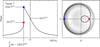Fig. 3 Response to a first-order resonance. Left panel: maximum eccentricity, emax, reached by a particle initially on a circular orbit with modified semimajor axis ∆ā/a0, with m < 0 and ϵ′ < 0. The right (resp. left) branch of the function is given by Eq. (29) (resp. 30). The value of emax suffers a discontinuity at Δā/a0 = (3/2)(m − 1)|2ϵ′|2/3, where emax jumps from |2ϵ′|1/3 to |16ϵ′|1/3, the maximum possible eccentricity, epeak. Right panel: phase portrait corresponding to the discontinuity, with the homoclinic trajectory going through the origin. The red and blue points correspond to their counterparts shown in the left panel.

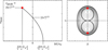Fig. 4 Same as Fig. 3, but for a second-order resonance. Left panel: function given by Eq. (33). The value of emax suffers a discontinuity at Δā/a0 = −|(m−2)ϵ′/2|, where emax jumps from zero to its maximum value, epeak = |4ϵ′|1/2. Right panel: phase portrait corresponding to the discontinuity. The red points correspond to their counterpart in the left panel.

6.2 Second-order resonances

For |Δā/a₀| > |(m − 2)ϵ′/2|, the origin of the phase portrait is a stable elliptic point (Sect. 4 and Fig. 2), so that e_max = 0 in this domain. Conversely, for |∆ā/a₀| ≤ |(m − 2)ϵ′/2|, the level curve going through the origin is an eight-shaped curve defined by ℋ(X, Y) = 0 (Fig. 1). Taking j = 2 in Eq. (10), we obtained $$\begin{array}{ll}{e}_{\max }=\sqrt{2\left|ϵ\prime \right|+\left(\frac{4}{m-2}\right)\frac{\Delta \overline{a}}{a_0}}\hfill & \text{for\hspace{0.17em}\hspace{0.17em}}\left|\frac{\Delta \overline{a}}{a_0}\right|\le \left|\frac{\left(m-2\right)ϵ\prime }{2}\right|,\hfill \\ e_{\max }=0\hfill & \text{for\hspace{0.17em}\hspace{0.17em}}\left|\frac{\Delta \overline{a}}{a_0}\right|>\left|\frac{\left(m-2\right)ϵ\prime }{2}\right|.\hfill \end{array}$$(33)

The value of e_max as a function of Δā/a₀ is plotted in Fig. 4 (left panel), with a discontinuity at ∆ā/a₀ = −|(m−2)ϵ′/2|. The phase portrait for that value is displayed in the right panel of Fig. 4.

The width over which e_max is nonzero and the value e_peak are now $$W=\left|\left(m-2\right)ϵ\prime \right|a_0\text{\hspace{0.17em}\hspace{0.17em}\hspace{0.17em}and\hspace{0.17em}\hspace{0.17em}\hspace{0.17em}}{e}_{\text{peak}}={\left|4ϵ\prime \right|}^{1/2}.$$(34)

The same exercise as for the first-order resonance provides the timescale, T_res, for building up the orbital eccentricity of a particle starting on a circular orbit with ā = 0. The origin of the phase portrait being a saddle point (Fig. 1), the particle moves away from this origin exponentially. Using again the equations of motions, Eq. (D.6), it can be shown that the e-folding timescale for the growth of eccentricity is $$T_{\text{res}}\approx \frac{4}{3\pi \left|m\left(m-2\right)ϵ\prime \right|}{T}_{\text{cor}}.$$(35)

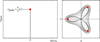Fig. 5 as Fig. 4, but for a third-order resonance. Left panel: function given by Eq. (36). Right panel: phase portrait corresponding to the discontinuity at ∆ā/a0 = 0. The red points correspond to their counterpart in the left panel.

6.3 Third-order resonances

The origin is an unstable hyperbolic point only for the isolated value ΔJ = ∆ā/a₀ = 0. Equation (10) then provides e_max through the equation $$-\frac{3}{4}{e}^4+ϵ\prime e^3\cos \left(3\varphi \right)=0.$$

This yields $$\{\begin{array}{ll}{e}_{\max }=\frac{4}{3}\left|ϵ\prime \right|\hfill & \text{for\hspace{0.17em}\hspace{0.17em}}\frac{\Delta \overline{a}}{a_0}=0\hfill \\ e_{\max }=0\hfill & \text{for\hspace{0.17em}\hspace{0.17em}}\frac{\Delta \overline{a}}{a_0}\ne 0\hfill \end{array}$$(36)

(see Fig. 5). Thus, for third-order resonances, we have $$W=0\text{\hspace{0.17em}\hspace{0.17em}\hspace{0.17em}and\hspace{0.17em}\hspace{0.17em}\hspace{0.17em}}{e}_{\text{peak}}=\frac{4}{3}\left|ϵ\prime \right|.$$(37)

We do not estimate here the resonant excitation time, T_res, for third-order resonances, as their width is zero, so that colliding particles cannot stay at exact resonance during the excitation process.

The values of W, e_peak, and the resonant excitation time, T_res, obtained for first-, second-, and third-order resonances are summarized in Table 1. This table also provides the dependence of these quantities with respect to the mass anomaly, µ, and the elongation parameter, C₂₂, of the body.

7 Resonance order and orbit structure

The response of a collisional disk to a SOR depends on two criteria: (i) the order of the resonance, which sets the typical eccentricities and the interval of ā over which a significant response of the disk is expected (Figs. 3 and 4); (ii) the structure of the periodic resonant orbits near the resonance, in particular the possible presence of self-intersecting points along these orbits, as observed in a frame rotating with the body.

This structure is entirely defined by the ratio n/Ω_B ≈ m/(m − j) (Eq. (4)). In particular, a resonant periodic orbit has |m′|(j′ − 1) self-intersecting points, where m′ and j′ are the relatively prime versions of m and j (Sicardy 2020; Sicardy et al. 2020). In a collisional disk, this implies that the resonant streamlines forced near a m/(m − j) SOR have |m′|(j′−1) self-crossing points. Thus, only the Lindblad resonances (j = j′ = 1) avoid the self-crossing problem (Fig. 6). This allows analytical solutions to be derived, with nested periodic neighboring orbits that interact to create spiral features. From this formalism, the description of angular momentum transfer and confinement mechanisms is possible. For j′ ≥ 2, a resonant streamline has at least one self-crossing point, where the density and velocity shear become undefined. A study of these cases requires numerical simulations, the topic of Paper II.

For higher-order resonances, the number of self-intersecting points of a periodic orbit depends on whether m and j are relatively primes. For instance, in the case of a triaxial body, only even values of m are allowed from the symmetry of the potential (Eq. (B.2)). Thus, the resonance n/Ω_B ≈ 1/2 is in fact a n/Ω_B ≈ 2/4 second-order resonance with m=−2 and j = 2. Even though the periodic orbit looks like that of a first-order resonance (in particular it has no self-intersection since m′=−1 and j′=1), it is actually a second-order resonant orbit, and as such will behave in the manner shown in Fig. 4.

Similarly, the n/Ω_B ≈ 1/3 resonance around a triaxial body is in fact a n/Ω_B ≈ 2/6 fourth-order resonance, but now the periodic orbits have one self-intersecting point, since m′ = −1 and j′ = 2 (Fig. 6). In summary, the structure of a resonant orbit alone is not sufficient to infer the order of the resonance. The order also depends on the symmetry of the potential at the origin of this resonance.

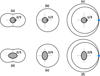Fig. 6 Examples of resonant periodic orbits. Panels a–c: case of a body with a mass anomaly, observed in a frame rotating with the body. Panels d–f: same, but around a triaxial body. Orbits (a) and (d) have the same structure and correspond to the same order of resonance. Orbits (b) and (e) have the same structure but correspond to different resonance orders (one and two, respectively). Orbits (c) and (ſ) have the same structure with one self-intersection point (blue dot) and are associated with resonances of orders two and four, respectively.

8 Applications to resonances around Chariklo, Haumea, and Quaoar

We now apply our results to Chariklo, Haumea, and Quaoar. Only first- and second-order resonances are considered, as they are the only ones that excite the orbital eccentricity, e, of an initially circular orbit over a finite interval of ā (see Figs. 3 and 4).

Two types of non-axisymmetric potentials are considered in this paper: a triaxial body that creates a quadrupole potential and a mass anomaly that creates a dipole-type potential.

The triaxial case assumes a homogeneous ellipsoid with principal semi-axes A > B > C, from which the elongation C₂₂ is derived (see Appendix B for additional details). The adopted physical parameters of Chariklo, Haumea, and Quaoar for the ellipsoid case are listed in Table 2 and have been used to generate Figs. 7, 8, and 9, showing a summary of the resonance and ring locations.

The mass anomaly case is described by a point-like mascon of mass µ relative to the body and located at the reference radius, R_ref, from the body center (see Table 2). No information is currently available for the values of µ concerning the three bodies. Here we adopt µ = 10⁻³ as a guideline because it corresponds in order of magnitude to the value that permits the confinement of material near the 1/3 SOR, based on the simulations presented in Paper II. As more information is gathered on Chariklo, Haumea, and Quaoar, the estimation of µ can be refined and the values of W and e_peak in Table 1 can be updated.

Figures 7, 8, and 9 show the eccentricities, e_max, raised by first- and second-order resonances around Chariklo, Haumea, and Quaoar. They are the functions shown in Figs. 3 and 4, relevant for each resonance. The resonant radii were calculated using the quadrupole gravitational potential in the ellipsoid case (see expression B.2) and the potential, −GM/r, in the mass anomaly case, together with the condition given by Eq. (3). Based on the values listed in Table 2, we also plot in Figs. 7, 8, and 9 the radii of the rings observed around the three bodies together with the nearby resonances 1/3 and, in the case of Quaoar, the location of the 5/7 SOR resonance that lies close to the ring Q2R.

8.1 Chariklo

Figure 7 displays trajectories of corotating particles encircling the fixed points C₂ and C₄. From Table 2, we obtain q^2/3 C₂₂ ~ 0.007. This value can be used to assess the dynamical stability of the corotation points C₂ and C₄, expressed by the condition F.6. Since it is not met (by a small margin), the points C₂ and C₄ are expected to be unstable. More accurate observations are needed to pin down the value of q^2/3 C₂₂, and thus more precisely assess the dynamical stability of Chariklo’s corotation points. We note that even if C₂ and C₄ are dynamically stable, they correspond in any case to local maxima of potential energy. As such, they are expected to be unstable against the dissipative effect of collisions, a conclusion that also holds for Haumea and Quaoar.

The Figure 7 reveals a dense mesh of first-order SORs bracketing the synchronous orbit. As is discussed in Sicardy et al. (2019), these resonances cause torques that rapidly clear the corotation zone, pushing material toward Chariklo inside the synchronous orbit and repelling that material toward outer regions outside the synchronous orbit. The clearing timescales are a few tens of years for resonances associated with Chariklo’s triaxiality, and a few million years for resonances associated with the mass anomaly of µ = 5 × 10⁻³ considered in Sicardy et al. (2019)³.

Moving outward, we see that the second-order 2/4 resonance associated with Chariklo’s triaxiality near the orbital radius 310 km induces large eccentricities of more than 0.2 on the particles, which prevents the presence of a stable ring in this zone. A more quiescent situation then sets in beyond the 2/4 resonance region. The second-order 1/3 resonance associated with a mass anomaly is then the only remaining one found in the pool of first-order or second-order resonances. With µ = 10⁻³, it excites a moderate eccentricity of 0.01. As was discussed earlier, the fourth-order 2/6 resonance associated with Chariklo’s triaxiality has a negligible effect on a ring in spite of a large value of ϵ_elon in Eq. (D.1). This is confirmed by N-body simulations of Paper II. Conversely, the simulations show the 1/3 resonance have a confining effect on a collisional disk, in spite of the expected streamline crossing problem.

We note that at the moment the uncertainty on the 1/3 resonance location (the purple region in Fig. 7) is consistent with Chariklo’s rings being trapped at the 1/3 resonance. A more accurate determination of the resonance location, deduced from a more accurate determination of Chariklo’s mass, is now needed to confirm this point.

8.2 Haumea

Figure 8 is the equivalent of Fig. 7 but for Haumea. We now have q^2/3 C₂₂ ~ 0.026 (Table 2), so that Haumea’s corotation points, C₂ and C₄, are unstable by a large margin from Eq. (F.6). This makes the entire corotation region of Haumea inappropriate for hosting rings. Moreover, Fig. 8 shows that the second-order resonance 2/4 raises eccentricities as high as 0.6. This makes the all region inside the radius ~2050 km inhospitable for rings. As in the case of Chariklo, the 1/3 SOR associated with a Haumea mass anomaly is the only one that induces moderate eccentricities (here on the order of 0.01), which may explain why a ring can be observed near that resonance.

8.3 Quaoar

Table 2 now provides q^2/3 C₂₂ ~ 0.0009, so that from Eq. (F.6) Quaoar’s corotation points, C₂ and C₄, shown in Fig. 9 appear to be safely stable. Concerning the SORs, the fact that Quaoar is a slower rotator than Chariklo and Haumea places these resonances farther out, when compared to the radius of the body. Consequently, Quaoar generally has a quieter environment than those of Chariklo and Haumea, due to a less dense mesh of resonances. However, the first- and second-order resonances associated with Quaoar’s triaxiality still excite large eccentricities, as do the first-order SORs associated with a putative Quaoar mass anomaly of µ = 10⁻³.

We see in Fig. 9 that Quaoar’s rings Q1R and Q2R are both close to second-order SORs (1/3 and 5/7, respectively). Both resonances excite modest eccentricities well below 0.01, assuming that µ = 10⁻³. We note that although Q1R is formally outside the purple region defining the possible radial location of the 1/3 SOR, the mismatch is at the 2.4σ level when accounting for the error bars, so it remains marginally significant.

The ring Q1R is also coincident (at the 1σ level) with the inner fifth-order 6/1 mean motion resonance (MMR) with the satellite Weywot (Fig. 9). The respective effects of the Weywot 6/1 MMR and the 1/3 Quaoar’s SOR depend on Weywoťs orbital eccentricity, e_w, and on Quaoar’s mass anomaly, µ, respectively (Morgado et al. 2023). Concerning Weywot, only an upper limit, e_w ≲ 0.034, is currently available (Braga-Ribas et al. 2025). With e_w ~ 0.005 and µ ~ 10⁻³ the 6/1 MMR and the 1/3 SOR excite comparable eccentricities on ring particles, so that none of them can a priory be neglected compared to the other (Morgado et al. 2023). More detailed calculations by Rodríguez et al. (2023) show that in the case of an orbital eccentricity of Weywot, a multiplet of six MMRs appears near the orbit of Q1R, possibly causing a clumping of particles in arcs. These effects are not considered in this paper, as we restrict our analysis to flrst-and second-order resonances.

Concerning Q2R, its radius coincides (below the 1σ level) with the location of the second-order 5/7 SOR. This resonance is actually bracketed by the stronger first-order resonances 3/4 and 2/3, a topic numerically discussed in Paper II.

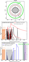Fig. 7 Resonances around Chariklo. Upper panel: trajectories (shown by light gray lines) around the corotation points, C2 and C4, of Chariklo, using Eq. (F.3). The dark gray ellipse is a pole-on view of Chariklo’s shape, taken from Table 2. The two green circles mark the radii of C1R and C2R rings. Red circle: First-order 2/3 resonance caused by Chariklo’s triaxial shape. Solid black circle: first-order 1/2 resonances caused by a mass anomaly. Dashed black circle: second-order 1/3 and 3/5 resonances caused by a mass anomaly. More resonances radii are plotted in the lower panels. Middle panel: maximum eccentricity, emax (in log-scale), reached by a particle initially on a circular orbit, reproducing the behavior displayed in Fig. 3 for each SOR. Red curves: SORs caused by the triaxial shape of Chariklo. Black curves: SORs caused by a mass anomaly, µ = 10−3. The orange box indicates Chariklo’s largest semi-axis, while the gray box shows the radial extension of the corotation zone, i.e., the full width of the corotation resonance (Eq. (F.4)). Lower panel: same, but for second-order resonances. The radii of the rings C1R and C2R are marked in green. The purple zone is the uncertainty on the 1/3 SOR location, due to the uncertainty on Chariklo’s mass. The uncertainties on the ring radii are negligible at this scale (see Table 2).

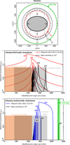Fig. 8 Same as Fig. 7, but for Haumea. Here we use the nomenclature H1R to be in line with the names of Chariklo’s and Quaoar’s rings (C1R, C2R, Q1R, and Q2R). The corotation zone now largely overlaps with the solid body. The uncertainty on the ring radius in the right panel is indicated by the green box, while the uncertainty on the 1/3 resonance radius is negligible at this scale (see Table 2).

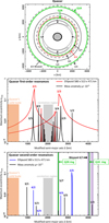Fig. 9 Same as Fig. 7, but for Quaoar, where two resonances have been added in the upper panel: the fifth-order resonance 6/1 with Weywot (the dotted circle close to Q1R), and the second-order resonance 5/7 with Quaoar, the dashed circle close to Q2R. As for Chariklo, the uncertainties on the 5/7 and 1/3 resonance radii (purple boxes in the lower panel) are larger than the uncertainties on the Q1R and Q2R ring radii (see Table 2).

9 Conclusions

This paper investigates from an analytical standpoint the behavior of test particles near j^th -order SORs between a non-axisymmetric body and test particles. We have estimated the stability of the corotation Lagrange points associated with the triaxial shape of Chariklo, Haumea, and Quaoar. Chariklo’s Lagrange points, C₁ and C₄ (Fig. 7), are marginally unstable, adopting the current knowledge of its shape. However, this may change as updated shape models are obtained. Conversely, Haumea’s Lagrange points (Fig. 8) are highly unstable, making the entire corotation region inhospitable for ring material. Finally Quaoar’s Lagrange points (Fig. 9) are dynamically stable and could support the presence of moonlets librating around the C₁ and C₄ points. However, in all of these cases, the C₁ and C₄ points correspond to maxima of potential, and are in principle unstable under the effect of dissipative collisions, unless energy is supplied by hypothetical moonlets as may be the case for Neptune’s ring arcs (Renner & Sicardy 2004; Renner et al. 2014; De Pater et al. 2018).

We have examined the topology of phase portraits for SORs of orders ranging from j = 1 to j = 5, the cases j > 5 being a mere repetition of what is observed for j = 5 (Fig. 1). This examination shows that only first-order Lindblad (j = 1) and second-order (j = 2) SORs can excite initially circular orbits. As such, they are the only ones that are expected to significantly disturb a dense collisional ring. In this context, we have estimated the characteristic widths as well as the typical eccentricities excited at these resonances (see Figs. 3 and 4, and Table 1).

Applications to Chariklo, Haumea, and Quaoar have been made. Concerning Chariklo and Haumea, the mesh of first-order and second-order SORs is dense, where the strong first-order resonances excite high orbital eccentricities. For these two bodies, this makes the region inside of the 1/2 (2/4 in the case of a triaxial body) SOR a strongly perturbed zone (Figs. 7 and 8). In that context, the second-order 1/3 resonance is the only one that does not excite high eccentricities, being at the same time separated from the perturbed region.

In the case of Quaoar, SORs are more widely separated, making its entire surroundings quieter compared to Chariklo and Haumea. Even so, the 2/1, 2/3, 1/2, and 2/4 SORs excite large eccentricities (Fig. 9) that should strongly perturb a ring. Conversely, the 5/7 and 1/3 second-order SORs (near the Q2R and Q1R rings, respectively) have a less drastic effect.

We show that, unlike for first-order resonances, the periodic orbits corresponding to second-order resonances have a self-crossing point (Fig. 6). This issue will be explored numerically in Paper II using N-body collisional simulations. In particular, we shall show that in spite of the self-crossing problem, ring confinement is in fact possible near the 1/3 resonance.

Acknowledgements

This work has been supported by the French ANR project Roche, number ANR-23-CE49-0012.

References

Appendix A Potential caused by a mass anomaly

A mass anomaly, µ, or mascon, introduces a dipole term with lowest values |m| = 1 in Eq. (1). This mass anomaly can reside at the surface of the object or be embedded in the body. To give a simple physical interpretation, it can be seen as a hemispheric mountain of height h > 0 or a depression of depth h < 0 located in the body equatorial plane at a characteristic distance R_ref (Eq. (B.1)) from the body center. Its mass relative to the body is then (noting that µ can be positive or negative), $$\mu ~\frac{1}{2}{\left(\frac{h}{R_{\text{ref}}}\right)}^3.$$(A.1)

This mass anomaly revolves at the spin rate of the body, Ω_B, so that (Sicardy et al. 2019; Sicardy 2020; Sicardy et al. 2020) $$\begin{array}{l}U\left(r\right)=-\frac{GM}{r}\hfill \\ -\frac{GM\mu }{R_{\text{ref}}}\left\{\frac{1}{2}{\displaystyle \sum _{m=-\infty }^{+\infty }\left[b_{1/2}^{\left(m\right)}\left(\frac{r}{R_{\text{ref}}}\right)-q{\delta }_{\left(\left|m\right|,1\right)}\left(\frac{r}{R_{\text{ref}}}\right)\right]\cos \left(m\theta \right)}\right\},\hfill \end{array}$$(A.2)

where $b_{1/2}^{\left(m\right)}$ is the classical Laplace coefficient, δ_{(|m|, 1)} is the Kronecker delta function that is associated with the indirect part of the potential and $$q=\frac{{\Omega }_{\text{B}}^2{R}_{\text{ref}}^3}{GM}$$(A.3)

is the rotational parameter.

The expression to be used in Eq. (7) is then $$U_m\left(\alpha \right)=-\left(\frac{GM\mu }{2R_{\text{ref}}}\right)\left[b_{1/2}^{\left(m\right)}\left(\alpha \right)-q{\delta }_{\left(\left|m\right|,1\right)}\alpha \right].$$(A.4)

Appendix B Potential of a triaxial homogeneous ellipsoid

We consider a homogeneous ellipsoid with principal semi-axes A, B and C. The elongation C₂₂ and the dynamical oblateness J₂ of the ellipsoid are given by Balmino (1994), $$C_{22}=\frac{A^2-B^2}{20R_{\text{ref}}^2}\text{\hspace{0.17em}\hspace{0.17em}\hspace{0.17em}and\hspace{0.17em}\hspace{0.17em}\hspace{0.17em}}{J}_2=-C_{20}=\frac{A^2+B^2-2C^2}{10R_{\text{ref}}^2},$$

where the reference radius R_ref is defined by $$\frac{3}{R_{\text{ref}}^2}=\frac{1}{A^2}+\frac{1}{B^2}+\frac{1}{C^2}.$$(B.1)

Following Boyce (1997), Sicardy et al. (2019), Sicardy (2020) and Sicardy et al. (2020) used the nonstandard parameters ${ϵ}_{\text{elon}}=\left(A^2+B^2\right)/2R_{\text{ref}}^2=10C_{22}$ and $f=\left(A^2+B^2-2C^2\right)/4R_{\text{ref}}^2=\left(5/2\right)J_2$ to characterize the elongation and the oblateness of the object, respectively. This avoided carrying the factors 10 and 5/2 in the various expressions of the potential. Another advantage of ϵ_elon and f was that they have simple physical interpretations when they approach zero, ϵ_elon ~ (A − B)/A and f = (A − C)/A.

Here we use the more standard parameters C₂₂ and J₂ to be in line with other works published in the literature, especially when obtained during flybys by space missions.

The quadrupole gravitational potential U(r) of the ellipsoid is derived from Balmino (1994) and (Boyce 1997), see also Sicardy et al. (2019), Sicardy (2020) and Sicardy et al. (2020). To zeroth order in J₂ (except for m = 0, see below), it reads $$U\left(r\right)=-\left(\frac{GM}{R_{\text{ref}}}\right){\displaystyle \sum _{-\infty }^{+\infty }{\left(\frac{R_{\text{ref}}}{r}\right)}^{\left|m\right|+1}{S}_{\left|m/2\right|}{\left(10C_{22}\right)}^{\left|m/2\right|}\cos \left(m\theta \right)}$$(B.2)

where only even values of m are allowed due to the π-symmetry of the ellipsoid. The factor S_p is recursively calculated through $$S_{p+1}=2\frac{\left(p+1/4\right)\left(p+3/4\right)}{\left(p+1\right)\left(p+5/2\right)}\times S_p,\text{\hspace{0.17em}\hspace{0.17em}\hspace{0.17em}with\hspace{0.17em}\hspace{0.17em}\hspace{0.17em}}{S}_0=1.$$

The expression B.2 shows from Eq. (1) that the term U_m(α) to be used in Eq. (7) is now $$U_m\left(\alpha \right)=-\left(\frac{GM}{R_{\text{ref}}}\right)\frac{{\left(10C_{22}\right)}^{\left|m\right|/2}{S}_{\left|m/2\right|}}{{\alpha }^{\left|m\right|+1}}.$$(B.3)

The axisymmetric part of the potential, corresponding to m = 0, is given in Sicardy et al. (2019) to any order in f. Keeping only the first-order term, we have $$U_0\left(r\right)=-\frac{GM}{r}\left[1+\frac{J_2}{2}{\left(\frac{R_{\text{ref}}}{r}\right)}^2\right],$$

from which the mean motion and epicyclic frequencies $$\begin{array}{l}{n}^2\left(r\right)=\frac{1}{r}\frac{d{U}_0\left(r\right)}{dr}=\frac{GM}{r^3}\left[1+\frac{3J_2}{2}{\left(\frac{R_{\text{ref}}}{r}\right)}^2\right]\hfill \\ {\kappa }^2\left(r\right)=\frac{1}{r^3}\frac{d\left(r^4{n}^2\right)}{dr}=\frac{GM}{r^3}\left[1-\frac{3J_2}{2}{\left(\frac{R_{\text{ref}}}{r}\right)}^2\right]\hfill \end{array}$$(B.4)

are derived. From these expressions, the location of the SOR resonances can be calculated using Eq. (3).

Appendix C Strengths of resonances

The strength of a resonance is quantified by the coefficient ϵ defined in Eq. (12). It is obtained using Eq. (7), where the operators F_N are given in Table C.1. They are listed according to the labels N used by Murray & Dermott (2000) and Ellis & Murray (2000). These operators contain both multiplicative factors and the derivative operators D = d/dα, D² = d² /dα²,…, D^j = d^j/dα^j for a given j, see Table C.1.

In the case of a homogeneous triaxial ellipsoid, the derivatives α^p D^p reduce to multiplicative factors because Um(α) depends only on powers of α (Eq. (B.3)), so that. α^p D^p = (−1)^p (|m| + 1)…(|m|+ p).

In the case of a mass anomaly, two terms appear in Eq. (A.4): the Laplace coefficients $b_{1/2}^{\left(m\right)}\left(\alpha \right)$ and the indirect term proportional to α. Thus, for the indirect term, all the derivatives α^p D^p for p ≥ 2 vanish. To obtain the derivative of the Laplace coefficients, we use the following recursive relations for p ≥ 1: $$\begin{array}{l}{D}^p{b}_{\gamma }^{\left(m\right)}=\hfill \\ \gamma \left[D^{p-1}{b}_{\gamma +1}^{\left(m-1\right)}+D^{p-1}{b}_{\gamma +1}^{\left(m+1\right)}-2\alpha D^{p-1}{b}_{\gamma +1}^{\left(m\right)}-2\left(p-1\right)D^{p-2}{b}_{\gamma +1}^{\left(m\right)}\right],\hfill \end{array}$$(C.1)

with the convention that D⁰ = 1.

Appendix D The Hamiltonian approach

Here we summarize and complement calculations made elsewhere (see e.g., Lemaitre (1984), Ferraz-Mello (1985), Murray & Dermott (2000), and El Moutamid et al. (2014)). The Hamiltonian describing the motion of the particle near a m/(m − j) resonance is $$H=-\frac{{\left(GM\right)}^2}{2{\Lambda }^2}+{\overline{U}}_{m,j}\left(\alpha \right){\left(\frac{2\Gamma }{\Lambda }\right)}^{j/2}\cos \left(j\varphi \right)-{\dot{\varpi }}_{\sec }\Gamma ,$$

where the resonant argument ϕ (which depends on m and j) is given by Eq. (11), and where $\Lambda =\sqrt{GMa}$ and $\Gamma =\sqrt{GMa}\left(1-\sqrt{1-e^2}\right)$. The pairs of conjugate variables of this Hamiltonian are then $$\begin{array}{l}\lambda \leftrightarrow J=\Lambda +\left(\frac{m-j}{j}\right)\Gamma \hfill \\ \varphi \leftrightarrow \Theta =\Gamma .\hfill \end{array}$$

As ℋ does not depends on λ, J is a constant of motion called the Jacobi constant. The actions Λ and J can be expanded near their values Λ₀ and J₀ at exact resonance, where $m{\Omega }_{\text{B}}-\left(m-j\right)n_0-j{\dot{\varpi }}_{\sec }=0$. Dropping constant terms, the Hamiltonian reads $$H=-\frac{3}{2a_0^2}{\left[J-J_0-\left(\frac{m-j}{j}\right)\Theta \right]}^2+{\overline{U}}_{m,j}\left(\alpha \right){\left(\frac{2\Theta }{{\Lambda }_0}\right)}^{j/2}\cos \left(j\varphi \right),$$

where ${\Lambda }_0=a-a_0^1{n}_0$ and $J-J_0=\left(a_0^2{n}_0/2\right)\left[\left(\Delta a/a_0\right)+\left(m-j/j\right)e^2\right]$, with ∆a = a − a₀. The first term in ℋ merely represents the Keplerian motion (slightly shifted by the precession term ${\dot{\varpi }}_{\sec }$), while the second term describes the perturbation induced by the resonance, at the lowest order j in eccentricity since Θ ∝ e².

The actions Λ₀, J − J₀ and Θ and the Hamiltonian can be normalized to $a_0^2{n}_0$. Adopting τ = n₀t as a new timescale, we obtain a one-degree of freedom Hamiltonian with new moment Θ = e²/2 and its conjugate angle ϕ, parameterized by the normalized Jacobi constant ∆J: $$\begin{array}{lll}H\left(\Theta ,\varphi \right)\hfill & =\hfill & -\frac{3}{2}{\left[\Delta J-\left(\frac{m-j}{j}\right)\Theta \right]}^2+ϵ{\left(2\Theta \right)}^{j/2}\cos \left(j\varphi \right)\hfill \\ \hfill & =\hfill & -\frac{3}{2}\left[\Delta J-\left(\frac{m-j}{2j}\right)e^2\right]+ϵe^j\cos \left(j\varphi \right),\hfill \end{array}$$(D.1)

where ϵ is given by Eq. 12 and ∆J = (1/2)[∆a/a₀ + ((m − j)/j)e²], see also Eq. 8. The parameter ∆J measures the distance of the orbits to exact resonance, and the equations of motion are now $$\{\begin{array}{l}\dot{\Theta }=-\frac{\partial H}{\partial \varphi }\hfill \\ \dot{\varphi }=+\frac{\partial H}{\partial \Theta },\hfill \end{array}$$(D.2)

where the dots denote the derivative with respect to τ, not t.

The Hamiltonian may also be written in terms of the mixed variables $$X=e\cos \left(\varphi \right)\text{\hspace{0.17em}\hspace{0.17em}\hspace{0.17em}and\hspace{0.17em}\hspace{0.17em}\hspace{0.17em}}Y=e\sin \left(\varphi \right),$$(D.3)

that define the eccentricity vector $$e=\left(X,Y\right).$$(D.4)

The last term of the Hamiltonian D.1 now contains the factor e^j cos(jϕ). Using the classical expansion $$\cos \left(j\varphi \right)={\displaystyle \sum _{k=0}^{\mathrm{int}\left(j/2\right)}{\left(-1\right)}^k{C}_j^k{\cos }^{j-2k}\left(\varphi \right){\sin }^{2k}\left(\varphi \right),}$$

where int(j/2) is the integer part of j/2 and $C_j^k=j!/k!\left(j-k\right)!$, we obtain $$\mathcal{H}\left(X,Y\right)=-\frac{3}{2}{\left[\Delta J-\left(\frac{m-j}{2j}\right)\left(X^2+Y^2\right)\right]}^2+ϵP\left(X,Y\right)$$(D.5)

where P(X, Y) is a homogeneous polynomial of degree j, $$P\left(X,Y\right)={\displaystyle \sum _{k=0}^{\mathrm{int}\left(j/2\right)}{\left(-1\right)}^k{C}_j^k{X}^{j-2k}{Y}^{2k}.}$$

The expressions of P(X, Y) are given in Table D.1 up to order j = 5. The equations of motion are now $$\{\begin{array}{l}\dot{X}=-\frac{\partial H}{\partial Y}\hfill \\ \dot{Y}=+\frac{\partial H}{\partial X}.\hfill \end{array}$$(D.6)

The phase portraits of resonances, i.e., the level curves of ℋ (Eq.D.5) are plotted in Fig. 1 for orders j ranging from one to five.

Appendix E The cubic equation

We give the classical expressions of the real roots of cubic equations reduced to their so-called depressed version $$z^3+pz+q=0,$$(E.1)

where (p, q) ∈ ℝ². The number of real solutions depends on the discriminant $$\Delta =-\left(4p^3+27q^2\right).$$(E.2)

For ∆ < 0, Eq. E.1 has a single real solution $$z={\left(\frac{-q-\sqrt{-\Delta /27}}{2}\right)}^{1/3}+{\left(\frac{-q+\sqrt{-\Delta /27}}{2}\right)}^{1/3}.$$(E.3)

Here and in all the paper, the cubic root of a real number is understood as the real root, i.e., discarding the two roots with imaginary parts.

For ∆ ≥ 0 (which requires p ≤ 0) Eq. E.1 has three real solutions $$z_k=2\sqrt{\frac{-p}{3}}\cos \left[\frac{1}{3}\arccos \left(\frac{3q}{2p}\sqrt{\frac{-3}{p}}\right)+\frac{2k\pi }{3}\right],$$(E.4)

Appendix F Potential near the corotating radius

F.1 Corotation trajectories

We consider the potential V(r) felt by a particle in the frame corotation with the body at angular velocity Ω_B, see Sicardy et al. (2019, 2020). Near the corotation radius a_cor, we have $$V\left(r\right)=U\left(r\right)-\frac{{\Omega }_{\text{B}}^2{r}^2}{2}~-{\Omega }_{\text{B}}^2{a}_{\text{cor}}^2\left[\frac{3}{2}{\left(\frac{\Delta r}{a_{\text{cor}}}\right)}^2+f\left(\theta \right)\right].$$(F.1)

In the case of a mass anomaly we have $$f\left(\theta \right)=q^{-1/6}\left(\frac{1}{\sqrt{q^{1/3}+q^{-1/3}-2\cos \theta }}-q^{1/2}\cos \theta \right)\mu$$

and in the case of an ellipsoid we have $$f\left(\theta \right)=2{\displaystyle \sum _{m=2}^{+\infty }{q}^{m/3}{S}_{m/2}{\left(10C_{22}\right)}^{m/2}\cos \left(m\theta \right)~3q^{2/3}{C}_{22}\cos \left(2\theta \right),}$$(F.2)

where only even values of m are allowed. The approximation above is obtained by retaining only the lowest-order term m = 2 (with S₁ = 0.15) in the summation, which is sufficient for order of magnitude considerations.

For typical values of µ and C₂₂, the corotation potential is largely dominated by C₂₂ (Sicardy et al. 2019), so we use the expression F.2 for f (θ). Near a_cor, and provided that the corotation point near the maximum of V(r) is dynamically stable, a particle with orbital semimajor axis a follows a trajectory defined by $$\frac{3}{8}{\left(\frac{\Delta a}{a_{\text{cor}}}\right)}^2+f\left(\theta \right)=\text{constant,}$$(F.3)

where ∆a = a − a_cor (Dermott & Murray 1981). In the ellipsoid case (Eq. F.2), this implies a corotation region of full width $$W_{\text{cor}}~8R_{\text{ref}}\sqrt{C_{22}}$$(F.4)

around the fixed points C₂ and C₄ displayed in Figs. 7, 8 and 9.

F.2 Stability of corotation points

The corotation points corresponding to local maxima of V(r) are linearly stable as long as (Murray & Dermott 2000) $${\left(4{\Omega }_{\text{B}}^2+V_{xx}+V_{yy}\right)}^2\le V_{xx}{V}_{yy}-V_{xy}^2.$$(F.5)

In the classical case of a mass anomaly with q = 1, this implies that the Lagrange points L₄ and L₅ are linearly stable if the Gascheau-Routh criterion µ ≤ 0.0385… is met. In our cases, q ≤ 1 (Table 2), so that even larger values of µ are required for L₄ and L₅ to be become unstable. From Eq. A.1, this would correspond for instance in Chariklo’s case to mountains of unrealistic heights h > 50 km. Thus, mass anomalies are not expected to create unstable corotation points L₄ and L₅.

In the ellipsoid case and using Eqs. F.1, F.2 and F.5, the points C₂ and C₄ are stable as long as $$q^{2/3}{C}_{22}\lesssim \mathrm{0.006.}$$(F.6)

All Tables

All Figures

Fig. 1 Representative phase portraits of resonances with orders j=1, 2, 3, 4, and 5, from top to bottom, respectively. Each phase portrait shows level curves of the Hamiltonians ℋ(X, Y) given in Eq. (D.5), where the mixed variables X and Y (Eq. (D.3)) define the eccentricity vector, e (Eq. (D.4)). The fixed elliptic points away from the origins correspond to maxima of ℋ(X, Y). For each resonance, four representative values of ∆J decreasing from left to right have been considered to illustrate the varying topologies of the phase portraits. The homoclinic trajectories are drawn in red. In all the plots, the value of the parameter ϵ appearing in Eq. (D.5) is taken as negative, as is the case for outer resonances. The topology of resonances with orders j > 5 are similar to the case j=5, except that there are j islands instead of five, with widths that decrease as j increases.

In the text

Fig. 2 Fixed points given by Eq. (16) as a function of ΔJ for resonances of various orders. They are the solutions of Eqs. (18), (20), (22), (24), and (26). In all the plots, the values of ϵ′ are taken as negative, as is the case for outer resonances. The cubic root, ϵ′1/3, is then understood as the real root, i.e., ignoring the complex roots. The blue (resp. red) branches corresponding to stable elliptic (resp. unstable hyperbolic) points. Similarly, blue (resp. red) dots at the origin indicate a stable (resp. unstable) point. The units of all the plots are arbitrary. Panel a: first-order resonances. The positions of two particular points are specified: the solution corresponding to ΔJ = 0 and the pitchfork bifurcation point at the lower right. Panel b: second-order resonances. The parabolic branches are the solutions of Eq. (20). The positions of three particular points are specified. Panel c: third-order resonances. The parabolic branches are the solutions of Eq. (22). The positions of three particular points are specified. The origin of the phase portrait (Xf = Ef =0) is stable everywhere, except for the value ΔJ = 0 (red dot), where it is hyperbolic. Panel d: fourth-order resonances. The parabolic branches are the solutions of Eq. (24). The origin of the phase portrait (Xf = Ef =0) is stable everywhere, except for large values of ϵ (see Eq. (14)). Panel e: resonances of orders j ≥ 5. In this case, Xf = Ef (Eq. (26)), so that the stability of the points corresponding to each branch cannot be indicated on the plot; hence, the black color used here. This plot is now indistinguishable from the unperturbed case (ϵ′ = 0).

In the text

Fig. 3 Response to a first-order resonance. Left panel: maximum eccentricity, emax, reached by a particle initially on a circular orbit with modified semimajor axis ∆ā/a0, with m < 0 and ϵ′ < 0. The right (resp. left) branch of the function is given by Eq. (29) (resp. 30). The value of emax suffers a discontinuity at Δā/a0 = (3/2)(m − 1)|2ϵ′|2/3, where emax jumps from |2ϵ′|1/3 to |16ϵ′|1/3, the maximum possible eccentricity, epeak. Right panel: phase portrait corresponding to the discontinuity, with the homoclinic trajectory going through the origin. The red and blue points correspond to their counterparts shown in the left panel.

In the text

	Fig. 4 Same as Fig. 3, but for a second-order resonance. Left panel: function given by Eq. (33). The value of emax suffers a discontinuity at Δā/a0 = −|(m−2)ϵ′/2|, where emax jumps from zero to its maximum value, epeak = |4ϵ′|1/2. Right panel: phase portrait corresponding to the discontinuity. The red points correspond to their counterpart in the left panel.
In the text

	Fig. 5 as Fig. 4, but for a third-order resonance. Left panel: function given by Eq. (36). Right panel: phase portrait corresponding to the discontinuity at ∆ā/a0 = 0. The red points correspond to their counterpart in the left panel.
In the text

Fig. 6 Examples of resonant periodic orbits. Panels a–c: case of a body with a mass anomaly, observed in a frame rotating with the body. Panels d–f: same, but around a triaxial body. Orbits (a) and (d) have the same structure and correspond to the same order of resonance. Orbits (b) and (e) have the same structure but correspond to different resonance orders (one and two, respectively). Orbits (c) and (ſ) have the same structure with one self-intersection point (blue dot) and are associated with resonances of orders two and four, respectively.

In the text

Fig. 7 Resonances around Chariklo. Upper panel: trajectories (shown by light gray lines) around the corotation points, C2 and C4, of Chariklo, using Eq. (F.3). The dark gray ellipse is a pole-on view of Chariklo’s shape, taken from Table 2. The two green circles mark the radii of C1R and C2R rings. Red circle: First-order 2/3 resonance caused by Chariklo’s triaxial shape. Solid black circle: first-order 1/2 resonances caused by a mass anomaly. Dashed black circle: second-order 1/3 and 3/5 resonances caused by a mass anomaly. More resonances radii are plotted in the lower panels. Middle panel: maximum eccentricity, emax (in log-scale), reached by a particle initially on a circular orbit, reproducing the behavior displayed in Fig. 3 for each SOR. Red curves: SORs caused by the triaxial shape of Chariklo. Black curves: SORs caused by a mass anomaly, µ = 10−3. The orange box indicates Chariklo’s largest semi-axis, while the gray box shows the radial extension of the corotation zone, i.e., the full width of the corotation resonance (Eq. (F.4)). Lower panel: same, but for second-order resonances. The radii of the rings C1R and C2R are marked in green. The purple zone is the uncertainty on the 1/3 SOR location, due to the uncertainty on Chariklo’s mass. The uncertainties on the ring radii are negligible at this scale (see Table 2).

In the text

	Fig. 8 Same as Fig. 7, but for Haumea. Here we use the nomenclature H1R to be in line with the names of Chariklo’s and Quaoar’s rings (C1R, C2R, Q1R, and Q2R). The corotation zone now largely overlaps with the solid body. The uncertainty on the ring radius in the right panel is indicated by the green box, while the uncertainty on the 1/3 resonance radius is negligible at this scale (see Table 2).
In the text

Fig. 9 Same as Fig. 7, but for Quaoar, where two resonances have been added in the upper panel: the fifth-order resonance 6/1 with Weywot (the dotted circle close to Q1R), and the second-order resonance 5/7 with Quaoar, the dashed circle close to Q2R. As for Chariklo, the uncertainties on the 5/7 and 1/3 resonance radii (purple boxes in the lower panel) are larger than the uncertainties on the Q1R and Q2R ring radii (see Table 2).

In the text

References

- Balmino, G. 1994, Celest. Mech. Dyn. Astron., 60, 331 [NASA ADS] [CrossRef] [Google Scholar]
- Boyce, W. 1997, Celest. Mech. Dyn. Astron., 67, 107 [NASA ADS] [CrossRef] [Google Scholar]
- Braga-Ribas, F., Sicardy, B., Ortiz, J. L., et al. 2014, Nature, 508, 72 [NASA ADS] [CrossRef] [Google Scholar]
- Braga-Ribas, F., Vachier, F., Desmars, J., Margoti, G., & Sicardy, B. 2025, Philos. Trans. Roy. Soc. Lond. A, 383, 20240200 [Google Scholar]
- De Pater, I., Renner, S., Showalter, M. R., & Sicardy, B. 2018, in Planetary Ring Systems. Properties, Structure, and Evolution, eds. M. S. Tiscareno, & C. D. Murray (Cambridge University Press), 112 [Google Scholar]
- Dermott, S. F., & Murray, C. D. 1981, Icarus, 48, 1 [NASA ADS] [CrossRef] [Google Scholar]
- El Moutamid, M., Sicardy, B., & Renner, S. 2014, Celest. Mech. Dyn. Astron., 118, 235 [Google Scholar]
- Ellis, K. M., & Murray, C. D. 2000, Icarus, 147, 129 [NASA ADS] [CrossRef] [Google Scholar]
- Ferraz-Mello, S. 1985, Celest. Mech., 35, 209 [Google Scholar]
- Leiva, R., Sicardy, B., Camargo, J. I. B., et al. 2017, AJ, 154, 159 [NASA ADS] [CrossRef] [Google Scholar]
- Lemaitre, A. 1984, Celest. Mech., 32, 109 [NASA ADS] [CrossRef] [Google Scholar]
- Morgado, B. E., Sicardy, B., Braga-Ribas, F., et al. 2021, A&A, 652, A141 [NASA ADS] [CrossRef] [EDP Sciences] [Google Scholar]
- Morgado, B. E., Sicardy, B., Braga-Ribas, F., et al. 2023, Nature, 614, 239 [NASA ADS] [CrossRef] [Google Scholar]
- Murray, C. D., & Dermott, S. F. 2000, Solar System Dynamics (Cambridge University Press) [Google Scholar]
- Ortiz, J. L., Gutiérrez, P. J., Sota, A., Casanova, V., & Teixeira, V. R. 2003, A&A, 409, L13 [NASA ADS] [CrossRef] [EDP Sciences] [Google Scholar]
- Ortiz, J. L., Santos-Sanz, P., Sicardy, B., et al. 2017, Nature, 550, 219 [NASA ADS] [CrossRef] [Google Scholar]
- Ortiz, J. L., Pereira, C. L., Sicardy, B., et al. 2023, A&A, 676, L12 [CrossRef] [EDP Sciences] [Google Scholar]
- Pereira, C. L., Braga-Ribas, F., Sicardy, B., et al. 2025, ApJ, 992, L19 [Google Scholar]
- Pereira, C. L., Sicardy, B., Morgado, B. E., et al. 2023, A&A, 673, L4 [NASA ADS] [CrossRef] [EDP Sciences] [Google Scholar]
- Pfenniger, D. 1984, A&A, 134, 373 [NASA ADS] [Google Scholar]
- Renner, S., & Sicardy, B. 2004, Celest. Mech. Dyn. Astron., 88, 397 [NASA ADS] [CrossRef] [Google Scholar]
- Renner, S., Sicardy, B., Souami, D., Carry, B., & Dumas, C. 2014, A&A, 563, A133 [NASA ADS] [CrossRef] [EDP Sciences] [Google Scholar]
- Rodríguez, A., Morgado, B. E., & Callegari, Jr., N. 2023, MNRAS, 525, 3376 [Google Scholar]
- Salo, H., & Sicardy, B. 2024, in European Planetary Science Congress, EPSC2024-534 [Google Scholar]
- Salo, H., & Sicardy, B. 2025, A&A, submitted (paper II) [Google Scholar]
- Salo, H., Sicardy, B., Mondino-Llermanos, A., et al. 2021, in European Planetary Science Congress, EPSC2021-338 [Google Scholar]
- Sicardy, B. 2020, AJ, 159, 102 [NASA ADS] [CrossRef] [Google Scholar]
- Sicardy, B., & Salo, H. 2024, in European Planetary Science Congress, EPSC2024-123 [Google Scholar]
- Sicardy, B., El Moutamid, M., Quillen, A. C., et al. 2018, in Planetary Ring Systems. Properties, Structure, and Evolution, eds. M. S. Tiscareno, & C. D. Murray (Cambridge University Press), 135 [Google Scholar]
- Sicardy, B., Leiva, R., Renner, S., et al. 2019, Nat. Astron., 3, 146 [NASA ADS] [CrossRef] [Google Scholar]
- Sicardy, B., Renner, S., Leiva, R., et al. 2020, in The Trans-Neptunian Solar System, eds. D. Prialnik, M. A. Barucci, & L. Young (Elsevier), 249 [Google Scholar]
- Sicardy, B., Salo, H., Souami, D., et al. 2021, in European Planetary Science Congress, EPSC2021-91 [Google Scholar]
- Sicardy, B., Braga-Ribas, F., Buie, M. W., Ortiz, J. L., & Roques, F. 2024, A&A Rev., 32, 6 [Google Scholar]
- Vachier, F., Berthier, J., & Marchis, F. 2012, A&A, 543, A68 [NASA ADS] [CrossRef] [EDP Sciences] [Google Scholar]
Unless otherwise mentioned, the energies and potentials used in this paper are given per unit mass.
To alleviate the notation, and because ϕ is used many times in this paper, we omit the indices m and j that should be attached to it. This should be remembered in all the expressions where ϕ appears.
Other clearing timescales are obtained knowing they scale like µ−2, since the torques at Lindblad resonances scale like µ2.