| Issue |
A&A
Volume 704, December 2025
|
|
|---|---|---|
| Article Number | A301 | |
| Number of page(s) | 11 | |
| Section | Planets, planetary systems, and small bodies | |
| DOI | https://doi.org/10.1051/0004-6361/202557173 | |
| Published online | 23 December 2025 | |
Secondary eclipses of two brown dwarfs in the K2 fields: Detection by multiple dataset merging
1
Konkoly Observatory, Research Center for Astronomy and Earth Sciences of HUN-REN, MTA Center of Excellence,
Budapest,
1121
Konkoly Thege ut. 15-17,
Hungary
2
Department of Physics & Astronomy, College of Charleston, Rita Hollings Science Center,
58 Coming Street,
Charleston,
SC
29421,
USA
3
Escuela Superior de Física y Matemáticas, Instituto Politécnico Nacional (IPN), Luis Enrique Erro S/N, San Pedro Zacatenco,
07738
Ciudad de México,
Mexico
★ Corresponding author: This email address is being protected from spambots. You need JavaScript enabled to view it.
Received:
9
September
2025
Accepted:
15
November
2025
Abstract
By using various data sources for the stellar fluxes in overlapping campaign fields and employing full time-series modeling, we report the detection of the secondary eclipses of two brown dwarfs (CWW 89Ab = EPIC 219388192b and HSHJ 430b = EPIC 211946007b). The detections yielded timings in agreement with the orbital elements derived from the earlier radial velocity measurements and eclipse depths of 70 ± 12 ppm (CWW 89Ab) and 852 ± 123 ppm (HSHJ 430b). While the high depth in the Kepler waveband for HSHJ 430b is in agreement with the assumption that the emitted flux mostly comes from the internal heat source and the absorbed stellar irradiation, the case of CWW 89Ab suggests a very high albedo because of the lack of sufficient thermal radiation in the Kepler waveband. Assuming a completely reflective dayside hemisphere, without circulation, the maximum value of the eclipse depth due to the reflection of the stellar light is 56 ppm. By making the extreme assumption that the true eclipse depth is 3σ less than the observed depth, the minimum geometric albedo becomes ~0.6.
Key words: methods: data analysis / planets and satellites: atmospheres / brown dwarfs
© The Authors 2025
 Open Access article, published by EDP Sciences, under the terms of the Creative Commons Attribution License (https://creativecommons.org/licenses/by/4.0), which permits unrestricted use, distribution, and reproduction in any medium, provided the original work is properly cited.
This article is published in open access under the Subscribe to Open model. This email address is being protected from spambots. You need JavaScript enabled to view it. to support open access publication.
1 Introduction
Being at the border of planets and “classical” stars, brown dwarfs (BDs) play a specific role in our understanding of both the evolution of very low-mass stars and the atmospheres of hot giant planets. Of particular interest are those BDs that are members of binary systems, and, especially, when they are also eclipsing systems. The apparent rarity of BDs within 5 AU of their main sequence hosts has led to the problem of the “brown dwarf desert”, as derived from early radial velocity surveys (Marcy & Butler 2000; Halbwachs et al. 2000). Although there has been a very spectacular increase in the number of transiting BD systems over the past several years, dominantly aided by the Transiting Exoplanets Survey Satellite (TESS, see Ricker et al. 2015), the BD desert phenomenon seems to survive (albeit with a lower contrast, see Carmichael et al. 2019; Stevenson et al. 2023; Vowell et al. 2025).
Secondary eclipse observations play a significant role in extrasolar planetary atmosphere science and it has a similar importance in the study of BDs. Due to their internal heat source, under favorable conditions, BDs are generally better candidates for secondary eclipse studies than close-in exoplanets, as the observed drop in the flux during the eclipse event is less dependent on the unknown (and usually low) geometric albedo. While this statement is true in the infrared, in the visible the situation might be more involved.
Despite their favorable position for occultation detections, the number of published successful detections is relatively low. Using the list of Barkaoui et al. (2025) and extending it by a few additional systems, within the classical BD mass limit of ~80 MJ, there are 55 objects. From these, eight systems have at least one successful secondary eclipse detection, with some of them in multiple wavebands (e.g., LHS 6343=KOI-959, see Frost et al. 2024). The purpose of this paper is to add two new detections to this list in the Kepler passband and investigate the possible constraints that these detections might pose on the orbit and, in particular, on the atmospheric properties (i.e., on the albedo).
The two systems to be investigated are members of nearby, deeply studied open clusters, and, therefore, we have well-defined ages, distances, and constraints on their chemical compositions. Age, in particular, is a prime factor in determining the basic physical parameters – mass, radius, and effective temperature (see, e.g., Baraffe et al. 2003). Consequently, the two systems discussed in this paper are among the most significant binaries with BD secondaries.
The number of transiting BD systems with a proven cluster membership is rather low. According to Acton et al. (2021), there are only three BD systems in clusters. Two of these are discussed in this paper, and a third one, RIK-72b (EPIC 205207894b), is in the Upper Scorpius OB association (David et al. 2019)1. This low number of transiting BDs in clusters is in contrast with the high number of BDs observed through imaging surveys of clusters.
The first system is CWW 89A (EPIC 219388192), a member of Ruprecht 147, a 2.67 Gyr old cluster. This is a triple system, with a solar-type main sequence host, and a distant outer companion (a likely M dwarf at ~25 AU, see Curtis et al. 2016; Nowak et al. 2017; Beatty et al. 2018). Interestingly, the observed eclipse depths in two Spitzer wavebands suggest a much higher internal temperature than current evolutionary models predict (see Beatty et al. 2018). Therefore, it is important to examine whether this discrepancy has any trace also at the shorter passband of Kepler as well.
The second system is HSHJ 4302 (EPIC 211946007), a member of the open cluster Praesepe. It consists of an M dwarf and a BD (Gillen et al. 2017). Here we present the first occultation detection for this system.
An integral part of the methodology employed in this paper is the utilization of the unique data availability for the K2 mission. The different approaches employed by various research groups to derive stellar fluxes enable us to search for shallow signals with greater success even in the case of single field target occupancy. Without the various aperture photometry sources and overlapping campaign fields (for EPIC 211946007), we could not detect the signals reported here (or, at least, their significance would have been far lower).
2 Method
There are three major steps in the analysis of each object. First, we treat the data on an author-by-author (hereafter source-by-source) and (campaign) field-by-field basis – see Sect. 3 for the specification of the individual datasets. Then, once all the time-series and statistical information is saved, these are fed into the data merging code that also performs the signal search on the averaged time series and statistics. Finally, in the third step, the single parameter (namely, δ2, the secondary eclipse depth in the Kepler passband Kp) is compared with the theoretical models and its consistency with other pieces of information is checked. We discuss the first two steps in the following subsections. More detailed discussion concerning the theoretical interpretation is postponed to Sect. 6.
2.1 Single time-series analysis
The data treatment and modeling of the single source, single field time series is akin to those employed in our earlier papers (Kovacs 2020, 2025), extended by the specific task of searching for eclipse features with the same orbital period and eclipse shape as the already known transit signal. The observed (Simple APerture – SAP) flux X(t) is approximated by the following additive signal model:
![Mathematical equation: $\[X(t)=F O U R(t)+S Y S(t)+O O T V(t)+T R(t)+E C(t).\]$](/articles/aa/full_html/2025/12/aa57173-25/aa57173-25-eq1.png) (1)
(1)
Here FOUR(t) is the Fourier representation of the stellar variability. This implies usually a high-order (i.e., mFOUR ~ 90) Fourier fit, with the frequencies of 1/T, 2/T, ..., mFOUR/T, where T stands for the full length of the given K2 observation campaign. We note that this is a general Fourier decomposition, and does not require the knowledge of the nature of the variability. It produces a reliable representation of nonstationarity, often present in stellar activity induced flux changes.
The corrections due to instrumental systematics are represented by S YS(t). This involves both common features in many stars in the same field (see, e.g., Smith et al. 2012) and those specific to the target (i.e., x, y pixel position- and bg background-dependent flux changes – see Bakos et al. 2010). The common systematics are derived from randomly selected stars, covering each CCD module roughly in equal number. These are passed through various non-variability criteria by ending up with some 500 non-variable stars for the full Kepler field of view. Next, an orthogonal set is built up from these time series with the aid of a Principal Component Analysis (PCA) routine, that yields also the order of “strength of commonality” via the eigenvalues of the PCA vectors. After a detailed experimentation, we found that using the first 100 PCA eigenvectors is an optimum choice to reach efficient eclipse signal detection.
The out-of-transit variation OOTV(t) is represented by a second-order Fourier sum (mOOTV = 2), allowing a rough modeling any phase and tidal variation with the orbital frequency and its first harmonic. It is important to note that although we introduce these orbital motion related variations, in the case of the two objects discussed in this paper, they will be largely eliminated by the high-order Fourier fit needed to tackle stellar variability, due to spots. Therefore, the derived OOTV(t) will be considered only as an additional correction function to eliminate non-eclipse-like variations related to the orbital motion.
The transit TR(t) is represented by a trapezoid with an U-shaped bottom part, similar as described by Kovacs (2020). The eclipse shape EC(t) is a flat-bottomed trapezoid with the same eclipse and ingress durations (respectively, t14 and t12) as those of the transit.
While the determination of the correction functions represented by the linear combinations of known functions is straight-forward via weighted least squares, that of {TR} and {EC} requires multistep methods. For {TR} we start from the roughly known transit parameters and employ a simple Monte Carlo (MC) method to sample the neighborhoods of those parameters. The period is fixed in this process, and taken as the average as given by our earlier analyses using the datasets dealt with in the present analysis.
In the case of the eclipse function {EC}, the situation is more complicated, because of the unknown eclipse phase. For this reason, first we need to compute the residual time series {Y}, left after the subtraction of all known signal constituents, namely, Y(t) = X(t) − FOUR(t) − S YS(t) − OOTV(t) − TR(t). Then, using the folded version of Y(t) (phased by the orbital period), we scan this function by shifting the trial eclipse center throughout the full orbital phase3 and fit the eclipse depth with the aid of weighted least squares. It is important to note that the determination of the weights is not part of the scanning process, but they are fixed and derived after each full iteration sequence, involving all known signal components. By considering the phase dependence of the fitted eclipse depth, we arrive to the Secondary Eclipse Search (SES) statistics, the basic information needed to make decision about the significance of the detection.
The decomposition shown by Eq. (1) is performed through an iterative scheme, during which we fit each entity separately4 by subtracting the other, already known (or estimated) functions from the input signal {X}. The iteration converges within ~10 iterations. The resulting time series is labeled as “reconstructed”, whereas the one that is the result of only one iteration cycle is referred to as “non-reconstructed”. Naturally, full reconstruction results in a better approximation of the transit (or other signal constituents – see Kovacs et al. 2005). Nevertheless, in the case of shallow signals, the component might be falsely identified and the reconstruction may amplify that misidentified noise components. Therefore, in faint signal search the examination of the statistics related to the non-reconstructed time series is also important.
For a quick summary, the procedures discussed in this subsection are shown in Fig. 1. Not shown in the figure, and not mentioned so far is the role of background stars. They may change the depth of the eclipse, and therefore, affect the success of the signal search on the averaged data and introduce additional error in the derived parameters. Therefore, a part of the analysis and preparation of the data input for the merging phase, is the determination of the hidden flux corrections for each dataset. This has been done by a trial and error method, whereby we used the thought to be most reliable transit depth determination and scaled all time series to yield the transit depth chosen. The size of the corrections were around a few percentages, but, due to the high-level of overall crowdedness of field C07, for EPIC 219388192, for some of the sources, the corrections were around 10% (see Appendix A for additional details).
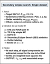 |
Fig. 1 Brief summary of the parameters and steps playing role in the analysis of the single datasets. See text for additional details. |
2.2 Multiple time-series analysis
Here the time series and SES statistics produced by the analysis of the target-, source-, and field-specified data (as described in Sect. 2.1) are fed into a code that combines these data for a given target with the goal of increasing the signal-to-noise ratio (SNR) of the unknown signal component. Due to their different meanings, time series and SES statistics are averaged differently. This allows us to compare the two results, serving as a sanity check for the final conclusion.
When averaging the SES statistics corresponding to the individual datasets, we focus on the possible signatures of a signal showing up in SES. The signal is exhibited as a dominant dip in this function. Therefore, it is meaningful to characterize the relevance of this particular SES, as the ratio between the largest dip (δ2) and the scatter (i.e., σ(SES), the standard deviation) of SES:
![Mathematical equation: $\[\mathrm{SNR}=\frac{\left|\delta_2-\langle\mathrm{SES}\rangle\right|}{\sigma(\mathrm{SES})},\]$](/articles/aa/full_html/2025/12/aa57173-25/aa57173-25-eq2.png) (2)
(2)
where ⟨⟩ denotes the average of SES. In computing ⟨SES⟩ and σ(SES), we exclude the phase range of ±t14/Porb around δ2, to avoid downward biasing of SNR. The eclipse depth δ2 is searched in a limited phase range (i.e., between 0.35 < φ < 0.65, a relatively close neighborhood of the expected phase of 0.50, in the case of zero eccentricity). Although this limitation of the search for δ2 introduces some bias in the final result (i.e., a preference toward low-eccentricity solutions), if the main dip in the restricted region is small, then the corresponding weight on the related SES will also be small. Therefore, the bias is expected to be small. The standard phase range above can be changed if there is sufficient evidence that the main dip is outside this range. In the two targets discussed in this paper, there was no such evidence.
The left part of Fig. 2 displays the simple process of SES weighting. The output parameters are δ2, the depth of the eclipse, and its phase, φ2 (relative to the phase of the transit, i.e., φ2 = ϕEC − ϕTR). One may also average the individual LCs, and then compute the SES of the average LC (see the right part of Fig. 2). While in the case of SES averaging we have arrays sampled at the same phase values, the LCs – even if they are folded – are not sampled in the same way. Therefore, we need not only to fold them, but also bin them on the same phase grid. We found that 1500 bins throughout the full orbital phase yield fine eclipse resolution and also, relatively few empty bins.
A natural way of averaging the above binned and folded LCs is to employ inverse variance weighting. The average LC will not carry any information about our preference of dip selection, as in the case of SES averaging. Because the unknown signal is weak, the variances are expected to be good approximations of the true variances. The average LC then undergoes of the standard SES analysis and another estimation is obtained for the two parameters (δ2 and φ2) of the secondary eclipse.
Although the different data sources yield somewhat different LCs, the associated stochastic components (naturally) are not independent (i.e., all sources have some common pixels while evaluating the total flux). Therefore, the noise averaging will not follow the classical ![Mathematical equation: $\[\sim 1 / \sqrt{n}\]$](/articles/aa/full_html/2025/12/aa57173-25/aa57173-25-eq3.png) law, but it will decrease with a lower pace as a function of the number of data sources. We found that the noise of the averaged LC is some 40–50% higher than expected from averaging independent random numbers. Even so, this milder improvement in the data quality is already quite significant, when the signal is at the verge of detectability for the single datasets.
law, but it will decrease with a lower pace as a function of the number of data sources. We found that the noise of the averaged LC is some 40–50% higher than expected from averaging independent random numbers. Even so, this milder improvement in the data quality is already quite significant, when the signal is at the verge of detectability for the single datasets.
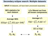 |
Fig. 2 Two types of approach in searching for a secondary eclipse by using multiple datasets (already filtered out from all other components – see Sect. 2.1 and Fig. 1). Left: averaging SES statistics of the individual datasets by their SNR. Right: averaging individual LCs by their inverse variance, and then compute SES of the average LC. The sum of the weights are normalized to unity in both cases. See text for more. |
3 Datasets
As described in Kovacs (2025), for K2, there are at least four easy to access datasets. All these sets were produced by using different methods in generating the raw time series from the long-cadence SAP fluxes. We employ these raw LCs from the following sources. Starting from the output of the pipeline of the mission, we downloaded the ASCII files from the IPAC exoplanet site5. These data are labeled by KEP. We note that Space Telescope Science Institute’s Mikulski Archive for Space Telescopes (MAST) site6 also hosts nearly the same data, but in our experience they contain far larger number of outliers, making the analysis more cumbersome and, ultimately, leaving more noise in the LCs. The next set by Petigura et al. (2015) (hereafter PET) comes from the earlier version of the NASA ExoFop site from the main Exoplanet Archive as cited earlier. The other two sets by Vanderburg & Johnson (2014) (VAN) and Luger et al. (2016, 2018) (LUG) have been downloaded from the corresponding MAST sites.
The list of datasets used in the time-series analysis is given in Table 1. All parameters refer to the residuals obtained from the non-reconstructed LCs (with reconstruction the parameters do not change at any significant degree). For C 18 we have only three sources, because of the incompleteness of the PET data for this campaign at the moment of download attempt at the IPAC ExoFop site. The two objects have drastically different noise levels, due to the large difference in their brightness (16.57 mag vs 12.34 mag in the Kepler filter for EPIC 211946007 and EPIC 219388192, respectively).
4 EPIC 219388192b
Here we present the search diagnostics both for the reconstructed and for the non-reconstructed time series. Likewise, the effect of multiple data sources is demonstrated both by averaging of the individual SES statistics and by running the same SES routine on the averaged LC. As discussed in Sect. 2.2, the latter comparison yields an additional test on the reliability of the detection, due to the difference between the ways how the averages were derived.
The parameters used in the analysis of the LCs of the individual sources were optimized for more efficient signal detection both by examining the result for the real data and by the recoverability of injected signals. These tests have led to slightly different parameter settings for the individual sources. For example, it turned out that for all sources, except for that of LUG, our method yields better LCs than those derived in the sources. As a result, for LUG only, we used the published, systematics-filtered LCs, instead of those derived by our code from LUG’s SAP time series. We followed this routine also for EPIC 211946007.
No pixel position induced flux corrections were needed in any of the datasets for EPIC 219388192, but PET became substantially less noisy by using time-dependent background correction. For LUG, we had to omit the first 50 most outlying points and cut the LC for the first three days.
We searched for eclipse signals in the averaged LCs derived both from the non-reconstructed and from the reconstructed LCs of the four sources. Figure 3 shows the individual and the averaged SES statistics derived from the non-reconstructed LCs. The averaged SES reaffirms the presence of a signal suspected, in particular, in the KEP dataset. This finding is further strengthened by the inspection of the same diagram, using SES statistics derived from the reconstructed LCs (that use full signal models, including the updated eclipse signal during the reconstruction process). Figure 4 shows the corresponding SES statistics. In agreement with our expectation, the signal shows up even more clearly in the averaged SES.
As discussed in Sect. 2.2, an important part of the signal confirmation is finding the same signal on the basis of the SES analysis of the averaged LCs. Showing only the final SES statistics, Fig. 5 exhibits the presence of the same signal, independently of the method used. The lower SNR of the SES based on the averaged LC is not surprising, since in employing this method, LCs with higher scatter are penalized (no information on a possible underlying signal is used), whereas in the case of SES averaging, the low-SNR SES statistics are weighted lower (suspected signal information is used).
The effect of averaging can also be exhibited by the LCs. Here we should use folded and binned LCs (see Sect. 2.2). Figure 6 shows both the neighborhood of the transit and the close proximity of the OOT level. The nearly zero scatter among the U-bottomed trapezoid fits (upper panel, black dots), shows the effectiveness of the hidden flux correction applied to the data of the individual sources (see Appendix A for details). Without this correction, the transit depths scattered about 5–10%. As expected, the scatter of the average LC is smaller than those of the separate source data (black vs gray points in the lower panel). However, because the individual time series are not independent, the RMS is greater than the statistical limit (70 ppm vs. 50 ppm).
Summary of the results obtained on the averaged SES statistics (method A) and those derived on the averaged LCs (method B) are given in Table 2. Because of the more involved nature of the eclipse depth error for method A, we give errors only for method B. Examining the derived parameters, the following trends can be observed. As expected, the reconstructed depths are larger, than the non-reconstructed depths, SNR-weighting for the SES statistics yields averaged SES with higher SNR than the one derived from the inverse variance weighted LCs. Preferring the complete signal modeling, but avoiding the chance of biased dip selection when method A is used, we settle on the result obtained by method B on the reconstructed LCs.
We see that all eclipse phases are the same for the various SES statistics, derived from the average LCs or individual SES statistics. Because the system has accurately measured radial velocity curves and subsequent analyses, it is possible to compare the above eclipse phase with those derivable from the spectroscopic orbital elements. Following Winn (2010) (his Eq. 33) and using the orbital elements ω and e by (Carmichael et al. 2019), we obtain7 φ2 = 0.617 ± 0.002. This is an excellent agreement, and lends an independent support of the reliability of the detected signal.
Basic properties of the input time series.
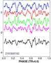 |
Fig. 3 SES statistics for the non-reconstructed LCs of EPIC 219388192. From top to bottom, plotted are SES statistics derived on the data sources of LUG, KEP, PET and VAN. The averaged SES is shown by black at the bottom. The phase scan is made from the transit center (phase zero) throughout the full orbital phase. All curves are plotted on the same (but arbitrary) scale and shifted properly for good visibility. |
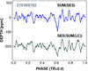 |
Fig. 5 Comparison of the final SES statistics obtained from averaging the individual SES statistics (top) with the one obtained from the averaged LC (bottom). As for the earlier, similar plots, we employed arbitrary vertical shifts for better visibility. The results shown are based on reconstructed LCs. |
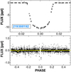 |
Fig. 6 Upper panel: binned transit for the merged, reconstructed LCs (gray), their U-bottomed trapezoid fits (black, binned, and averaged in the same way as the data). Lower panel: gray points as above, black points are the weighted averages of the gray points. The yellow line shows the best-fitting flat-bottomed trapezoid for the secondary eclipse. The stroboscopic effect (exhibiting as small gaps) is not visible in the lower panel, because of the extended horizontal scale. |
Secondary eclipse parameters for EPIC 219388192.
5 EPIC 211946007b
There are pros and cons for the detectability of the secondary eclipse of EPIC 211946007. First of all, the target is faint, leading to some 20 times higher noise than in the case of EPIC 219388192. In addition, the host star is an M dwarf, with low flux level and, therefore, the reflected light is expected to be low. However, being a member of the Praesepe cluster, the system is young, and therefore, the internal heat of the BD is expected to be high. Furthermore, the orbital period is only 1.983 days, yielding favorable irradiation in spite of the cool M dwarf host. And last, but not least, the star is in the overlapping region of three K2 fields, allowing to suppress the high noise by the substantial number of data sources, covering three independent visits of the target.
Because of the great similarity of the non-reconstructed and reconstructed SES statistics (see also EPIC 219388192), we show only the relevant plots obtained from the reconstructed LCs. The SES statistics derived from these LCs are shown in Fig. 7. It is clear that the signal is barely visible in most of the individual SES statistics. Due to the large number of data sources, and, importantly, to the field overlaps, the averaged statistics clearly exhibit the presence of a signal (more significantly, than in the case of EPIC 219388192).
Testing the detection by using LC averaging first, and SES analysis after, on the average LC, confirms the detection (see Fig. 8). The significant improvement on the LC quality due to averaging is exhibited in Fig. 9.
The resulting secondary eclipse parameters are shown in Table 3. Again, by using the orbital parameters of ω = 5° ± 20° and e = 0.146 ± 0.025 from Gillen et al. (2017) we arrive to φ2 = 0.593 ± 0.019. Although the error is larger than for EPIC 219388192, the actual RV measurement is in nice agreement with the value derived from the independent photometric data.
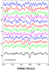 |
Fig. 7 SES statistics for the reconstructed LCs of EPIC 211946007. The structure of the figure is similar to that of Fig. 3. From top to downward, we show the SES statistics derived on the data sources of LUG, KEP, PET and VAN. This pattern is repeated (from top to bottom) for fields C05, C16 and C18 (for the latter, we have only LUG, KEP and VAN). Vertical shifting and scaling are applied as in Fig. 3. |
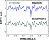 |
Fig. 8 Comparison of the final SES statistics obtained from averaging the individual SES statistics (top) with the one obtained from the averaged LC (bottom). The results shown are based on reconstructed LCs. |
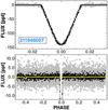 |
Fig. 9 Upper panel: binned transit for the merged, reconstructed LCs (gray), and their U-bottomed trapezoid fits (black, averaged in the same way as the data). Lower panel: gray points as above, black points are the weighted averages of the gray points. The yellow line shows the best-fitting flat-bottomed trapezoid for the secondary eclipse. |
Secondary eclipse parameters for EPIC 211946007.
6 Comparison with evolution and atmosphere models
In addition to giving an independent constraint on the eccentricity via the phase of the secondary eclipse, the depth of the eclipse is also a useful measure of the atmospheric properties of the companion. In particular, once the temperature of the companion is known, for example, from other eclipse measurements in the infrared, the geometric albedo Ag can be estimated. The total eclipse depth can be represented as follows (see, e.g., Cowan & Agol 2011; Daylan et al. 2021)
![Mathematical equation: $\[\delta_{\text {obs }}=\delta_{\text {refl }}+\delta_{\text {therm }}.\]$](/articles/aa/full_html/2025/12/aa57173-25/aa57173-25-eq4.png) (3)
(3)
Because of the internal energy source in the case of BDs, the second term (that includes also the absorbed stellar flux) yields an important contribution to the observed eclipse depth – in particular, in the infrared wavebands. Considering that the eccentricity for these BDs are not negligible, the eclipse depth, associated with the reflected light, is related to the geometric albedo Ag through the following relations
![Mathematical equation: $\[\delta_{\mathrm{refl}}=A_{\mathrm{g}}\left(\frac{R_{\mathrm{c}}}{r_{\mathrm{occ}}}\right)^2, r_{\mathrm{occ}}=\frac{a\left(1-e^2\right)}{1-e ~\sin~ \omega},\]$](/articles/aa/full_html/2025/12/aa57173-25/aa57173-25-eq5.png) (4)
(4)
where Rc is the radius of the companion (i.e., that of the BD), a is the semi-major axis, e is the eccentricity, ω is the argument of the periapsis and rocc is the distance of the companion from the star at the moment of the occultation. Although not shown explicitly, Ag is wavelength-dependent, leading to effective reflectivity at short wavelengths, and rather ineffective reflectivity further down in the infrared regime. We approximately take this dependence into consideration by using the models employed on the occultation data of HD 189733b by Krenn et al. (2023). Their Fig. 6 is used to estimate the efficiency of the reflection of the incident stellar flux as a function of wavelength and overall (gray) Ag values. Their result implies that the amount of the reflected flux is less than ~20% in the Spitzer wavebands than that of in the Kepler waveband even if the gray geometric albedo is as high as 75% in the Kepler waveband.
The secondary eclipse depth due to the reradiation part of the stellar flux and the internal energy source is given by
![Mathematical equation: $\[\delta_{\text {therm }}=\left(\frac{R_{\mathrm{c}}}{R_{\mathrm{s}}}\right)^2 \frac{F_{\mathrm{c}}\left(\lambda, T_{\text {day }}\right)}{F_{\mathrm{s}}(\lambda)}.\]$](/articles/aa/full_html/2025/12/aa57173-25/aa57173-25-eq6.png) (5)
(5)
Here Rs is the stellar radius, Fc and Fs are the fluxes of the companion and the star respectively and λ is the wavelength. The day-side companion temperature Tday depends on the temperature generated by the internal heat source Tint and on Tirr, the temperature originating from the non-reflected part of the stellar irradiation. We relate these temperatures following, for instance, Amaro et al. (2023)
![Mathematical equation: $\[T_{\text {day }}^4=T_{\mathrm{irr}}^4+T_{\mathrm{int}}^4.\]$](/articles/aa/full_html/2025/12/aa57173-25/aa57173-25-eq7.png) (6)
(6)
To compute Tirr, we follow the customary parameterization (i.e., Cowan & Agol 2011)
![Mathematical equation: $\[T_{\mathrm{irr}}^4=\alpha T_0^4, \alpha=\left(1-A_{\mathrm{B}}\right)\left(\frac{2}{3}-\epsilon \frac{5}{12}\right),\]$](/articles/aa/full_html/2025/12/aa57173-25/aa57173-25-eq8.png) (7)
(7)
where the substellar temperature T0 due to stellar irradiation can be evaluated with the knowledge of the stellar effective temperature Ts
![Mathematical equation: $\[T_0=T_{\mathrm{s}} \sqrt{R_{\mathrm{c}} / r_{\mathrm{occ}}}.\]$](/articles/aa/full_html/2025/12/aa57173-25/aa57173-25-eq9.png) (8)
(8)
The absorbed heat is controlled by the Bond albedo AB, whereas the efficiency of the day- to the night-side circulation is determined by the parameter ϵ. Although the effect of the stellar irradiation on Tday is under 4% for both objects studied in this paper, we use Tday as given by Eq. (6) for the effective temperature of the BD atmosphere models, partially accounting for the effect of stellar irradiation on the theoretical spectra.
The Bond albedo is a highly involved quantity (e.g., Marley et al. 1999) and it is hard to relate to the geometric albedo in a precise way. Nevertheless, the two types of albedos are obviously related. To take this relation into consideration in a rather approximate way, we considered two classes of objects. First we examined 15 solar system bodies as collected at the corresponding Wikipedia site8 (see also Cox 2000, for the planets). Omitting Haumea and Enceladus, we found Ag ~ 1.1AB, with a substantial standard deviation of ~0.1. Then we took the hot Jupiter sample of Schwartz & Cowan (2015) (their Table 4, with fully corrected Ag and assumed gray planet atmosphere (columns five and eight, respectively). Here we found a very tight correlation for the 11 planets, but with a lower slope of ~0.8. Considering that this estimate is based on relatively early sets of hot Jupiter atmospheric observations, and that the solar system albedos can be regarded as less relevant for BDs, we think that the Ag = AB approximation in the Kepler waveband can be a reasonable one in the context of this paper. In any case, the specific relation of Ag and AB has only a moderate effect on the final conclusion, due to the high value of Tint and the high power used for the temperature components in calculating the planet temperature (see Eq. (6)).
To utilize the above formulae in the estimation of the theoretical eclipse depths, we need stellar and substellar atmosphere models yielding the corresponding spectra as they appear in Eq. (5). We note that the simple black body fluxes perform rather poorly, because of the significant molecular bands in the substellar, and, for similar reason, in the low stellar mass regimes. For the stellar spectra we used the Kurucz2003 (Castelli & Kurucz 2003) and BT-NextGen models by Allard et al. (2012). For the two BD systems and for the wavelength regime used, they yield very similar results. For the companions we took the quite recent ATMO models by Phillips et al. (2020). These are “clear” (i.e., non-cloudy), nonirradiated models with chemical equilibrium and solar composition. For a brief justification of our choice of cloudless models without stellar irradiation we note the following.
Beatty et al. (2018) used irradiated cloudy and cloudless models for EPIC 219388192. In the left panel of their Fig. 8 the cloudless, but irradiated models reach a maximum eclipse depth of ~1600 ppm between the two Spitzer passbands. Using their preferred internal temperature of 1700 K with the same atmospheric conditions (low AB of 1%, no day- to the night-side heat redistribution), we get an eclipse depth of 1500 ppm. One can get an exact agreement with their model value by increasing Tint to 1800 K, but we think that this is well within the subtle differences of the theoretical models and do not influence our broad estimate of the geometric albedo of the BD component, the focus point of this work.
For using cloudless models, we again refer to Fig. 8 of Beatty et al. (2018). Comparing the left (“clear”) and right (“cloudy”) spectra, we see that there is a ~10% reduction in the emitted flux for the cloudy models. Similarly, we infer from a brief inspection of Fig. 10 from Morley et al. (2024) that the effect of clouds near to the optical part of the emission spectrum may also not exceed ~10%.
Importantly, there are also evolution models that yield theoretical values for Tint, directly related to the observed secondary eclipse depths. Because this estimate comes from the independently measured companion mass, radius, age and assumed chemical composition, the derived Tint value is very important in harmonizing evolutionary and atmosphere models with the observations. To predict Tint from models, we used the very recent SONORA models by Davis et al. (2025) (see also Marley et al. 2021). For comparison, we also utilized the earlier models of Baraffe et al. (2003). We used linear and quadratic interpolations both for the atmosphere and for the evolutionary models to match the input parameters exactly. Because of the deeper than expected eclipse depths, for Tirr we assumed that the day-to-night heat transport is ineffective, namely, ϵ = 0. This is in agreement with the approach of Beatty et al. (2018) and also supported by the low efficiency of the energy transport suggested by the secondary eclipse observations at 2 μm of Hot Jupiters (Kovacs & Kovacs 2019).
In the following subsections we examine the constraints put on the geometric albedos by the above relations. In this comparison we do not intend to perform a full-scale modeling (e.g., comparing various atmospheric compositions), because: firstly, it is out of the scope of the paper, and, secondly, and even more importantly, the limited data (too few spectral points with low accuracy in relatively wide filter bands) would not justify such a deep study.
 |
Fig. 10 Theoretical emission spectra transformed to eclipse depth for EPIC 219388192b (CWW 89Ab). Only the thermal components are included (internal and absorbed stellar sources). Blue: Tint = 1900 K – fit to the Spitzer data within 1σ; gray: Tint = 944 K – BD evolutionary temperature. For the star we used the BT-NextGen models (Allard et al. 2012), whereas for the BD we employed the ATMO models of Phillips et al. (2020). Green horizontal bars show the theoretical depths in the Spitzer wavebands. Red dots with error bars show the observed depths by Beatty et al. (2018). The third red dot in the left bottom corner is the eclipse depth in the Kp filter. The inset zooms in on this region, indicating the expected eclipse depth for the reflectivity levels shown. Horizontal error bars indicate the equivalent filter width. See text for further details. |
6.1 The high geometric albedo of EPIC 219388192b
Together with the Spitzer observations, we have three secondary eclipse measurements for this object: with depths 1147 ± 213 ppm (at 3.5 μm) and 1097 ± 225 ppm at 4.4 μm9 as given by Beatty et al. (2018) and 70 ± 12 ppm at 0.6 μm from the analysis presented in this paper. Based on its cluster membership, the age is reasonably fixed at 2.67 ± 0.47 Gyr (i.e., Torres et al. 2021). From the system analysis, Carmichael (2023) obtained 39.2 ± 1.1 MJ for the mass of the BD component. By using these values, from the SONORA models we get RBD = 0.91 RJ, in excellent agreement with the observed value of 0.94 ± 0.02 given by Carmichael (2023). From the same models, for Tint we get 944 K. Using this Tint and assuming AB = 0.6, from the ATMO models we get the spectrum shown in Fig. 10 by a gray line. We see that with the evolutionary internal temperature, the measured Spitzer fluxes are several sigmas apart from the fluxes predicted by the BD atmosphere models. Because of the relatively low value of Tint and the proximity of the host star, it matters how the Bond albedo is chosen10.
In the example shown in Fig. 10, the Bond albedo was chosen to yield the 3σ low limit of the observed eclipse depth in the Kp band, and, assuming that the AB = Ag condition holds. Allowing AB varying freely between 0.1 and 0.9, the corresponding predicted eclipse depths vary in 225–59 ppm (at 3.5 μm) and in 522–267 ppm (at 4.4 μm). In both extremes the theoretical fluxes significantly underestimate the observed values, especially in the shorter waveband. These results support the observation of Beatty et al. (2018) that EPIC 219388192b shows serious overluminosity with respect to the evolutionary models.
By tuning upward Tint, we can match the observed Spitzer fluxes quite closely. By scaling the peak flux to the same value as in the models of Beatty et al. (2018), we find that for the ATMO models we need to set Tint by 200 K higher than the one preferred by Beatty et al. (2018). With Tint = 1900 K, we can fit the Spitzer fluxes within 1σ. Of course, depending on the accepted accuracy within which the fit is considered to be acceptable, a lower Tint value is also possible, but from the current Spitzer data the disagreement between the evolutionary and observed internal temperatures seems to be quite solid.
As seen in Fig. 10, the theoretical thermal flux has negligible contribution at the Kepler waveband even at the high temperature required by the Spitzer data. It follows that the only way to produce the observed eclipse depth is if the geometric albedo is high. The inset in Fig. 10 shows the relation between the observed and theoretically expected eclipse depths. At Ag = 1.0, the expected eclipse depth is 59 ppm. In the extreme case, if the depth is overestimated by 3σ, that is, its value is not 70 ppm, but only 34 ppm, the resulting Ag is 0.57, which is still remarkably high. It is worth noting that KELT-1b may have also a similarly large reflectivity in the TESS band according to Beatty et al. (2020), although this has been challenged recently by the reanalysis of the TESS data by von Essen et al. (2021) and the inclusion of the CHEOPS observations by Parviainen et al. (2022). Some of these discrepancies may be attributed to seasonal variations in the reflective clouds of KELT-1b (i.e., Parviainen 2023).
6.2 The unconstrained albedo of EPIC 211946007b
Unfortunately, for this system, the only secondary eclipse data available to us are those presented in this paper. Because the single, short-waveband eclipse depth is insufficient to derive Tint, we must rely on the evolutionary models. Since this target is also a cluster member we can follow the same steps as in the case of EPIC 219388192. Being a member of the Praesepe, the age of the system is 0.64 ± 0.02 Gyr (Morales et al. 2022). From the system analysis (Carmichael 2023) we have 54.6 ± 6.8 MJ for the mass of the BD component. From these data the SONORA models yield RBD = 1.01 RJ, within 1σ of the observed value of 0.95 ± 0.07 RJ (Carmichael 2023). The match also yields Tint = 1624 K.
The observed eclipse depth in the Kp band is 852 ± 123 ppm. With Tint as above and assuming “standard” low Ag of 0.1, and apply the AB = Ag assumption, we get a depth of 511 ppm, which is within 3σ of the observed value. We need to increase Ag to 0.6 to come within the 1σ neighborhood of the observed value. Alternatively, we may assume that Tint is slightly underestimated by the models (indeed, Baraffe et al. 2003, yields 200 K higher value). Allowing an increase of only 100 K in Tint and setting Ag = 0.2, we arrive at 797 ppm, well within the 1σ limit of the observed eclipse depth. If we assume complete heat redistribution (i.e., ϵ = 1, instead of 0, as we assumed throughout the paper), then, with the same Ag, we get a depth of 775 ppm, again in good agreement with the observed depth. We conclude that the available data for EPIC 211946007b are not in contradiction with the low albedo, standard evolutionary internal temperature scenario.
For completeness, in Fig. 11 we show the emission spectrum of EPIC 211946007 for Tint = 1724 K and Ag = 0.1 together with the observed eclipse depth as given in this paper. For the first sight it may look inconsistent that the integrated theoretical emission in the neighborhood of 0.6 μm can indeed reach the value of the observed flux. However, a closer examination of the Kp filter function shows that although the transmission decreases considerably outside the effective waveband (shown by the horizontal bars in the figure), the emission sharply increases in these regions and this compensates for the decrease in the filter transmission. The comparison of Figures 10 and 11 shows that while topologically the two spectra are very similar, because of the substantially younger age of EPIC 211946007b, its overall thermal emission is much higher than that of EPIC 219388192b. This difference allows the low albedo scenario quite more likely for EPIC 211946007b.
 |
Fig. 11 As in Fig. 10 (same theoretical models and figure setting), but for EPIC 211946007b (HSHJ 430b). We used 100 K higher internal temperature (i.e., Tint = 1724 K) than the theoretical evolutionary value. The green horizontal bar in the inset shows the theoretical depth in the Kepler waveband, assuming 10% Bond albedo. Red dots with error bars show the observed depth. |
7 Conclusions
The earlier perception on the low occurrence rate of brown dwarf companions in short-period binaries (Marcy & Butler 2000; Halbwachs et al. 2000) seems to be considerably modified by the increasing number of discoveries during the past decade. The contribution of the TESS satellite to these discoveries is especially spectacular. More than half of the currently known ~55 BDs in eclipsing binary systems have been discovered by transit searches on the photometric time series based on the observations made by TESS. The followup observations generally yield orbital elements and masses, but secondary eclipse detections are relatively rare, in spite of the expected higher signal-to-noise ratio (with respect to the thermal emission of planets). Secondary eclipse observations are instrumental in the verification of atmospheric and evolutionary model predictions.
We used multiple datasets to detect the secondary eclipses of two binaries hosting BDs. Both systems were observed by K2 (the Kepler two-wheel mission) and reside in well-known open clusters. In addition, there are several independent photometric datasets available for both systems. Furthermore, EPIC 211946007 (HSHJ 430) was observed during three different K2 campaigns.
Once the variabilities due to instrumental systematics, stellar spots and transits were filtered out, the data were searched for secondary eclipses on data source and campaign field bases. Then, the separate secondary eclipse search statistics were merged to increase the signal-to-noise ratio of the detected signal. To verify the consistency of the method and to obtain another estimate of the eclipse signal, we performed similar data merging for the light curves. In these two approaches the averaging relies on different pieces of information of the constituent datasets. Therefore, checking the consistency of the results is a significant step in confirming the reliability of the detections. The main results of the paper can be summarized as follows.
EPIC 219388192 (CWW 89A) shows a secondary eclipse with a depth of (70 ± 12) ppm. The thermal emission (even at the excessive internal temperature predicted from the Spitzer observations by Beatty et al. 2018) is not enough in the Kp band to explain this depth. Therefore, it seems unavoidable to conclude that this BD is also peculiar in that it has a high geometric albedo. The minimum albedo allowed by the eclipse depth is 0.6. Obviously, independent measurements at short wavebands would be quite important to confirm or refute our finding.
EPIC 211946007 (HSHJ 430) did not have a secondary eclipse observation before this report. We detected a depth of (852 ± 123) ppm which, due to the young age of the system, can be produced (almost entirely) by internal heat. Therefore, the “standard” low-albedo scenario is quite likely for the BD component of this system.
Acknowledgements
We thank the referee for the thorough and instructive report which contributed to the improvement of the clarity of the paper. This work has been inspired by the TESS III Science Conference held at MIT in July, 2024. Discussions with Theron Carmichael, Dave Latham, Avi Shporer, Jon Jenkins and Eric Feigelson were very stimulating. The help given by Melanie A. Swain regarding the usage of the current ExoFOP site is greatly appreciated. The availability of independently obtained photometric time series was essential in the successful detections presented in this paper. Thanks are due to Eric Petigura, Andrew Vanderburg and Rodrigo Luger for making their data accessible to the public. This research has made use of the NASA/IPAC Infrared Science Archive, which is funded by the National Aeronautics and Space Administration and operated by the California Institute of Technology. This research has made use of the Spanish Virtual Observatory (https://svo.cab.inta-csic.es) project funded by MCIN/AEI/10.13039/501100011033/ through grant PID2020-112949GB-I00. This paper includes data collected by the Kepler mission and obtained from the MAST data archive at the Space Telescope Science Institute (STScI). Funding for the Kepler mission is provided by the NASA Science Mission Directorate. STScI is operated by the Association of Universities for Research in Astronomy, Inc., under NASA contract NAS 5-201326555.
References
- Acton, J. S., Goad, M. R., Burleigh, M. R., et al. 2021, MNRAS, 505, 2741 [NASA ADS] [CrossRef] [Google Scholar]
- Allard, F., Homeier, D., & Freytag, B. 2012, RSPTA, 370, 2765 [Google Scholar]
- Amaro, R. C., Apai, D., Zhou, Y., et al. 2023, ApJ, 948, 129 [Google Scholar]
- Bakos, G. Á., Torres, G., Pál, A., et al. 2010, ApJ, 710, 1724 [NASA ADS] [CrossRef] [Google Scholar]
- Baraffe, I., Chabrier, G., Barman, T. S., et al. 2003, A&A, 402, 701 [Google Scholar]
- Barkaoui, K., Sebastian, D., Zúniga-Fernández, S., et al. 2025, A&A, 696, 44 [Google Scholar]
- Beatty, T. G., Morley, C. V., Curtis, J. L., et al. 2018, AJ, 156, 168 [NASA ADS] [CrossRef] [Google Scholar]
- Beatty, T. G., Wong, I., Fetherolf, T., et al. 2020, AJ, 160, 211 [Google Scholar]
- Carmichael, Theron W. 2023, MNRAS, 519, 5177 [NASA ADS] [CrossRef] [Google Scholar]
- Carmichael, T. W., Latham, D. W., & Vanderburg, A. M. 2019, AJ, 158, 38 [NASA ADS] [CrossRef] [Google Scholar]
- Castelli, F., & Kurucz, R. L. 2003, IAUS, 210, A20 [NASA ADS] [Google Scholar]
- Cowan, N. B., & Agol, E. 2011, ApJ, 729, 54 [Google Scholar]
- Cox, A. N. 2000, Allen’s Astrophysical Quantities, 4th edn. (New York: AIP Press; Springer) [Google Scholar]
- Curtis, J., Vanderburg, A., Montet, B., et al. 2016, The 19th Cambridge Workshop on Cool Stars, Stellar Systems, and the Sun (CS19), Uppsala, Sweden, 06-10 June 2016, id. 95 [Google Scholar]
- David, T. J., Hillenbrand, L. A., Gillen, E., et al. 2019, ApJ, 872, 161 [Google Scholar]
- Davis, C. E., Fortney, J., Iyer, A., et al. 2025, https://doi.org/10.5281/zenodo.15611937 [Google Scholar]
- Daylan, T., Günther, M. N., Mikal-Evans, T., et al. 2021, AJ, 161, 131 [NASA ADS] [CrossRef] [Google Scholar]
- Frost, W., Albert, L., Doyon, R., et al. 2024, ApJ, 972, 199 [Google Scholar]
- Gillen, E., Hillenbrand, L. A., David, T. J., et al. 2017, ApJ, 849, 11 [Google Scholar]
- Halbwachs, J. L., Arenou, F., Mayor, M., et al. 2000, A&A, 355, 581 [NASA ADS] [Google Scholar]
- Howell, Steve B., Sobeck, Charlie, Haas, Michael, et al. 2014, PASP, 126, 398 [NASA ADS] [CrossRef] [Google Scholar]
- Kovacs, G. 2020, A&A, 643, 169 [Google Scholar]
- Kovacs, G. 2025, A&A, 699, 20 [Google Scholar]
- Kovacs, G., & Kovacs, T. 2019, A&A, 625, 80 [Google Scholar]
- Kovacs, G., Bakos, G., & Noyes, R. W. 2005, MNRAS, 356, 557 [CrossRef] [Google Scholar]
- Krenn, A. F., Lendl, M., Patel, J. A., et al. 2023, A&A, 672, A24 [NASA ADS] [CrossRef] [EDP Sciences] [Google Scholar]
- Luger, R., Agol, E., Kruse, E., et al. 2016, AJ, 152, 100 [Google Scholar]
- Luger, R., Kruse, E., Foreman-Mackey, D., et al. 2018, AJ, 156, 99 [Google Scholar]
- Marcy, G., & Butler, P. 2000, PASP, 112, 137 [NASA ADS] [CrossRef] [Google Scholar]
- Marley, M. S., Gelino, C., Stephens, D., et al. 1999, ApJ, 513, 879 [NASA ADS] [CrossRef] [Google Scholar]
- Marley, M. S., Saumon, D., Visscher, C., et al. 2021, ApJ, 920, 85 [NASA ADS] [CrossRef] [Google Scholar]
- Morales, L. M., Sandquist, E. L., Schaefer, G. H., et al. 2022, AJ, 164, 34 [NASA ADS] [CrossRef] [Google Scholar]
- Morley, C. V., Mukherjee, S., Marley, M. S., et al. 2024, ApJ, 975, 59 [NASA ADS] [CrossRef] [Google Scholar]
- Nowak, G., Palle, E., Gandolfi, D., et al. 2017, AJ, 153, 131 [Google Scholar]
- Parviainen, H. 2023, A&A, 671, L3 [NASA ADS] [CrossRef] [EDP Sciences] [Google Scholar]
- Parviainen, H., Wilson, T. G., Lendl, M., et al. 2022, A&A, 668, A93 [NASA ADS] [CrossRef] [EDP Sciences] [Google Scholar]
- Petigura, E. A., Schlieder, J. E., Crossfield, I. J. M., et al. 2015, ApJ, 811, 102 [Google Scholar]
- Phillips, M. W., Tremblin, P., & Baraffe, I., et al. 2020, A&A, 637, 38 [Google Scholar]
- Ricker, G. R., Winn, J. N., Vanderspek, R., et al. 2015, JATIS, 1, 014003 [Google Scholar]
- Schwartz, J. C., & Cowan, N. B. 2015, MNRAS, 449, 4192 [NASA ADS] [CrossRef] [Google Scholar]
- Smith, J. C., Stumpe, M. C., Van Cleve, J. E., et al. 2012, PASP, 124, 1000 [Google Scholar]
- Stevenson, A. T., Haswell, C. A., Barnes, J. R., et al. 2023, MNRAS, 526, 5155 [NASA ADS] [CrossRef] [Google Scholar]
- Torres, G., Vanderburg, A., Curtis, J. L., et al. 2021, ApJ, 921, 133 [Google Scholar]
- Vanderburg, A., & Johnson, J. A. 2014, PASP, 126, 948 [Google Scholar]
- von Essen, C., Mallonn, M., Piette, A., et al. 2021, A&A, 648, A71 [NASA ADS] [CrossRef] [EDP Sciences] [Google Scholar]
- Vowell, N., Rodriguez, J. E., Quinn, S. N., et al. 2023, AJ, 165, 268 [NASA ADS] [CrossRef] [Google Scholar]
- Vowell, N., Rodriguez, J. E., Latham, D. W., et al. 2025, AJ, 170, 68 [Google Scholar]
- Winn, J. N. 2010, arXiv e-prints [arXiv:1001.2010] [Google Scholar]
By examining the list of Barkaoui et al. (2025), we also found that HIP 33609 is a member of the MELANGE-6 association (Vowell et al. 2023).
We use the name suggested by SIMBAD (https://simbad.cds.unistra.fr/simbad/) for the apparently nontraditional earlier naming of AD 3116, that is simply a record number assigned by the VizieR team.
Although the U-bottomed transit approximation works well in most cases, for the sake of the more sensitive shallow secondary eclipse, we mask out the transit phase by substituting {Y} with a Gaussian noise of the same standard deviation as the rest of {Y}.
Except for {SYS} and {FOUR}, that are fitted jointly.
Because of its tiny effect (10−4 in orbital phase units) we omitted the light-time effect for both systems discussed in this paper.
We note that Beatty et al. (2018) use mean wavelength, whereas we use effective wavelength; the latter are shorter by 0.1 μm.
We recall that, meanwhile, the reflective component at the Spitzer passband remains small – less than 10 ppm.
Appendix A Average flux correction
Due to the variation of the background star contamination because of the different aperture masks, the different data sources yield different transit depths. We considered this effect at the stage of data input. For a given data source, object and K2 campaign number, we applied the following type of correction to the input SAP fluxes FLX:
![Mathematical equation: $\[F L X_c=F L X \times f_c /<F L X>,\]$](/articles/aa/full_html/2025/12/aa57173-25/aa57173-25-eq10.png) (A.1)
(A.1)
where < FLX > is the robust average of the input flux and fc is the correction factor. This factor is set by a trial and error approximation by inspecting the final data product – resulting from the various noise and signal filtering steps (see Sect. 2.1). In Table A.1 we summarize the set-by-set values of fc. The factors were chosen so that the respective transit depths be the same for the given target, independently of the data source. We used the following transit depths for the two targets. For EPIC 219388192: δ1 = 0.0104 and for EPIC 211946007: δ1 = 0.1400.
Input flux correction factors.
All Tables
All Figures
|
Fig. 1 Brief summary of the parameters and steps playing role in the analysis of the single datasets. See text for additional details. |
| In the text | |
|
Fig. 2 Two types of approach in searching for a secondary eclipse by using multiple datasets (already filtered out from all other components – see Sect. 2.1 and Fig. 1). Left: averaging SES statistics of the individual datasets by their SNR. Right: averaging individual LCs by their inverse variance, and then compute SES of the average LC. The sum of the weights are normalized to unity in both cases. See text for more. |
| In the text | |
|
Fig. 3 SES statistics for the non-reconstructed LCs of EPIC 219388192. From top to bottom, plotted are SES statistics derived on the data sources of LUG, KEP, PET and VAN. The averaged SES is shown by black at the bottom. The phase scan is made from the transit center (phase zero) throughout the full orbital phase. All curves are plotted on the same (but arbitrary) scale and shifted properly for good visibility. |
| In the text | |
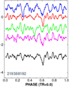 |
Fig. 4 As in Fig. 3, but for the reconstructed LCs. |
| In the text | |
|
Fig. 5 Comparison of the final SES statistics obtained from averaging the individual SES statistics (top) with the one obtained from the averaged LC (bottom). As for the earlier, similar plots, we employed arbitrary vertical shifts for better visibility. The results shown are based on reconstructed LCs. |
| In the text | |
|
Fig. 6 Upper panel: binned transit for the merged, reconstructed LCs (gray), their U-bottomed trapezoid fits (black, binned, and averaged in the same way as the data). Lower panel: gray points as above, black points are the weighted averages of the gray points. The yellow line shows the best-fitting flat-bottomed trapezoid for the secondary eclipse. The stroboscopic effect (exhibiting as small gaps) is not visible in the lower panel, because of the extended horizontal scale. |
| In the text | |
|
Fig. 7 SES statistics for the reconstructed LCs of EPIC 211946007. The structure of the figure is similar to that of Fig. 3. From top to downward, we show the SES statistics derived on the data sources of LUG, KEP, PET and VAN. This pattern is repeated (from top to bottom) for fields C05, C16 and C18 (for the latter, we have only LUG, KEP and VAN). Vertical shifting and scaling are applied as in Fig. 3. |
| In the text | |
|
Fig. 8 Comparison of the final SES statistics obtained from averaging the individual SES statistics (top) with the one obtained from the averaged LC (bottom). The results shown are based on reconstructed LCs. |
| In the text | |
|
Fig. 9 Upper panel: binned transit for the merged, reconstructed LCs (gray), and their U-bottomed trapezoid fits (black, averaged in the same way as the data). Lower panel: gray points as above, black points are the weighted averages of the gray points. The yellow line shows the best-fitting flat-bottomed trapezoid for the secondary eclipse. |
| In the text | |
|
Fig. 10 Theoretical emission spectra transformed to eclipse depth for EPIC 219388192b (CWW 89Ab). Only the thermal components are included (internal and absorbed stellar sources). Blue: Tint = 1900 K – fit to the Spitzer data within 1σ; gray: Tint = 944 K – BD evolutionary temperature. For the star we used the BT-NextGen models (Allard et al. 2012), whereas for the BD we employed the ATMO models of Phillips et al. (2020). Green horizontal bars show the theoretical depths in the Spitzer wavebands. Red dots with error bars show the observed depths by Beatty et al. (2018). The third red dot in the left bottom corner is the eclipse depth in the Kp filter. The inset zooms in on this region, indicating the expected eclipse depth for the reflectivity levels shown. Horizontal error bars indicate the equivalent filter width. See text for further details. |
| In the text | |
|
Fig. 11 As in Fig. 10 (same theoretical models and figure setting), but for EPIC 211946007b (HSHJ 430b). We used 100 K higher internal temperature (i.e., Tint = 1724 K) than the theoretical evolutionary value. The green horizontal bar in the inset shows the theoretical depth in the Kepler waveband, assuming 10% Bond albedo. Red dots with error bars show the observed depth. |
| In the text | |
Current usage metrics show cumulative count of Article Views (full-text article views including HTML views, PDF and ePub downloads, according to the available data) and Abstracts Views on Vision4Press platform.
Data correspond to usage on the plateform after 2015. The current usage metrics is available 48-96 hours after online publication and is updated daily on week days.
Initial download of the metrics may take a while.