| Issue |
A&A
Volume 704, December 2025
|
|
|---|---|---|
| Article Number | A12 | |
| Number of page(s) | 16 | |
| Section | Stellar structure and evolution | |
| DOI | https://doi.org/10.1051/0004-6361/202557188 | |
| Published online | 26 November 2025 | |
Rare find: Discovery and chemo-dynamical properties of two s-process-enhanced RR Lyrae stars
1
Department of Physics, University of Rome Tor Vergata, Via della Ricerca Scientifica 1, 00133 Rome, Italy
2
INAF Osservatorio Astronomico di Padova, Vicolo dell’Osservatorio 5, 35122 Padova, Italy
3
Department of Astronomy & McDonald Observatory, The University of Texas at Austin, 2515 Speedway, Austin, TX 78712, USA
4
Departament de Física Quàntica i Astrofísica, Universitat de Barcelona, c. Martí i Franquès, 1, 08028 Barcelona, Spain
5
Konkoly Observatory, HUN-REN Research Centre for Astronomy and Earth Sciences, MTA Centre for Excellence, Konkoly Thege Miklós út 15-17, Budapest 1121, Hungary
6
MTA-ELTE Lendület “Momentum” Milky Way Research Group, Szent Imre h. u. 112, 9700 Szombathely, Hungary
7
Eötvös Loránd University, Institute of Physics and Astronomy, H-1117 Pázmány Péter sétány 1/A, Budapest, Hungary
8
School of Physics and Astronomy, Monash University, Clayton, VIC 3800, Australia
9
OzGrav: Australian Research Council Centre of Excellence for Gravitational Wave Discovery, Clayton, VIC 3800, Australia
10
INAF – Osservatorio Astronomico di Roma, Via Frascati 33, Monte Porzio Catone, Italy
11
Space Science Data Center – ASI, Via del Politecnico SNC, 00133 Rome, Italy
12
Department of Physics, North Carolina State University, Raleigh, NC 27695, USA
13
Max-Planck-Institut fur Astronomie, Konigstuhl 17, D-69117 Heidelberg, Germany
⋆ Corresponding author: This email address is being protected from spambots. You need JavaScript enabled to view it.
Received:
10
September
2025
Accepted:
16
October
2025
Abstract
Aims. We report the serendipitous discovery of two RR Lyrae stars that exhibit significant s-process element enrichment, a rare class previously represented solely by TY Gruis. Our goal is to characterise these objects chemically and dynamically, and explore their origins and evolutionary histories.
Methods. Using high-resolution spectroscopy from HERMES@AAT and UVES@VLT, we derived detailed chemical abundances of key s-process elements (Y, Ba, La, Ce, Nd, and Eu) and carbon, along with α elements (Ca, Mg, and Ti). We also employed Gaia Data Release 3 astrometric data to analyse their kinematics, orbital properties, and classify their Galactic population membership. We compared observational results with theoretical asymptotic giant branch (AGB) nucleosynthesis models to interpret their enrichment patterns.
Results. Both stars exhibit clear signatures of s-process enrichment, with significant overabundances in second-peak elements such as Ba and La compared to first-peak Y and Zr. Comparison with AGB nucleosynthesis models suggests their progenitors experienced pollution of s-process-rich material, consistent with early binary interactions. However, notable discrepancies in dilution factors highlight the need for more refined low-metallicity AGB models. We also explore and discuss alternative scenarios, including sub-luminous post-AGB-like evolution or double episodes of mass transfer. In the latter case, the star initially undergoes a mass transfer when it is on the main sequence, accreting material from a former AGB companion. Subsequently, as the star evolves along the red giant branch, it may again transfer mass to its companion before becoming an RR Lyrae star.
Conclusions. Our findings confirm the existence of s-process-enhanced RR Lyrae stars and demonstrate the importance of combining chemical and dynamical diagnostics to unveil their complex evolutionary pathways. Future detailed binary evolution modelling and long-term orbital monitoring are essential to resolve their formation scenarios and assess the role of binarity in the evolution of pulsating variables.
Key words: stars: abundances / stars: AGB and post-AGB / stars: atmospheres / binaries: general / stars: variables: RR Lyrae
© The Authors 2025
 Open Access article, published by EDP Sciences, under the terms of the Creative Commons Attribution License (https://creativecommons.org/licenses/by/4.0), which permits unrestricted use, distribution, and reproduction in any medium, provided the original work is properly cited.
This article is published in open access under the Subscribe to Open model. This email address is being protected from spambots. You need JavaScript enabled to view it. to support open access publication.
1. Introduction
Stellar nucleosynthesis involves multiple pathways operating across a range of stellar masses and the synthesis of different elements. Light metals (from carbon to zinc) are primarily produced via charged-particle fusion within stellar cores and shells. In contrast, the formation of elements beyond the iron peak (Fe-group) is dominated by neutron-capture (n-capture) processes, which are classified based on the n-capture timescale relative to radioactive decay: the slow (s-) process, which predominantly occurs in asymptotic giant branch (AGB) stars, and the rapid (r-) process, associated with highly energetic astrophysical sites such as type II supernovae and neutron star mergers (Burbidge et al. 1957; Sneden et al. 2008; Cowan et al. 2021; Lugaro et al. 2023).
Evolved stars with unusual abundance patterns in very light and/or heavy elements serve as natural laboratories for studying nucleosynthesis pathways. Among these, Barium (Ba) stars (Bidelman & Keenan 1951) are a prominent class characterised by strong spectral lines of s-process1 elements like Sr, Y, Ba, La, and others. They are generally G- or K-type dwarfs and giants with effective temperatures between approximately Teff = 4000 − 6000 K. Their peculiar chemical abundance patterns (for their evolutionary state), coupled with radial velocity variations indicating binarity, support the hypothesis that Ba stars have accreted s-process-enriched material from former AGB companions, now white dwarfs, in binary systems (McClure et al. 1980; Jorissen et al. 1998). This mass transfer scenario explains the surface enrichment despite the stars’ evolutionary stages being unrelated to the production of such elements internally.
Detailed spectroscopic analyses, using high-resolution and high signal-to-noise observations, have revealed significant correlations between s-process element abundances and metallicity, as well as insights into the nucleosynthetic conditions in their progenitor AGB stars. Studies comparing observed abundance ratios (such as [hs/ls], between heavier and lighter s-process elements2) with theoretical models support low-mass (≈2−4 M⊙) AGB stars as the primary sites of s-process nucleosynthesis involved in Ba star formation (de Castro et al. 2016; Cseh et al. 2018, 2022; Roriz et al. 2021, 2024; Yang et al. 2024). Furthermore, the orbital properties of Ba systems, including their period-eccentricity distributions, have been extensively studied to better constrain models of binary evolution and mass transfer (Jorissen et al. 2016, 2019; Krynski et al. 2025). Beyond classical Ba stars, related objects such as CH stars and carbon-enhanced metal-poor (CEMP) stars extend this paradigm to different stellar populations. CH stars, which are similar to Ba stars but generally have a lower metallicity, are also members of binary systems where s-process enhancement results from past mass transfer during the AGB phase of a companion (Keenan 1942; McClure & Woodsworth 1990). CEMP stars, particularly the CEMP-s subclass, show large carbon enhancements ([C/Fe] > +0.7), accompanied by s-process element overabundances, and are typically very metal-poor stars. The binary nature of many CEMP-s stars has been well established and has been found to support their formation via mass transfer processes akin to those in Ba and CH stars (Lucatello et al. 2005; Abate et al. 2015; Hansen et al. 2016; Jorissen et al. 2016). Understanding the properties of these chemically peculiar stars not only sheds light on the nucleosynthetic processes within AGB stars but also probes the formation and evolution of binary and multiple star systems across different stellar populations.
While Ba/CH/CEMP-s stars are observed among giants and unevolved stars (occurrence rate ≲1%), TY Gruis (Preston et al. 2006) stood as the sole identified s-process-enhanced, carbon-rich RR Lyrae (RRL). Low-mass stars undergoing helium burning on the Hertzsprung-Russell (HR) diagram horizontal branch will cross the instability strip (IS) and become RR Lyrae pulsating variables during this transition (Catelan 2004, and references therein). Their defining characteristics include short-period brightness variations (from several hours to less than a day) and pulsations in the fundamental (RRab), first overtone (RRc), or both modes simultaneously (RRd; Catelan 2007; Soszyński et al. 2011). The astrophysical significance of RRLs stems from their prevalence in old stellar populations (Iben 1974; Preston et al. 2019), well-established period-luminosity relations that enable precise distance determination (Longmore et al. 1986; Bono et al. 2011; Braga et al. 2021), and readily distinguishable light curve morphologies (Bailey 1902; Jurcsik & Kovacs 1996; Smolec 2005). RRL stars display a broad spectrum of chemical compositions, from metallicities as low as 1/1000 of solar to solar. Moreover, while metal-poor and extremely metal-poor RRL stars are characterised by α enhancements (Hansen et al. 2011; D’Orazi et al. 2025), metal-rich RRLs exhibit subsolar α-element abundances (Chadid et al. 2017; D’Orazi et al. 2024). This finding has motivated the development of alternative evolutionary pathways, such as binary interactions (e.g. Karczmarek et al. 2017; Bobrick et al. 2024).
Preston et al. (2006) conducted an extensive examination of the metal-poor ([Fe/H] ≈ −2.0 ± 0.2) RRL TY Gruis and discovered substantial carbon and n-capture element excesses that are suggestive of mass transfer from a former AGB companion. Unfortunately, the presence of the Blazhko effect complicated radial velocity measurements and hindered the search for orbital evidence of a binary system.
This paper presents the serendipitous discovery of two additional s-process-rich RR Lyrae stars, which expand the known population beyond the single previous detection by Preston et al. (2006) and extend it towards higher metallicities. The paper is structured as follows. Section 2 details the sample selection, observational methods, and abundance analysis procedures. In Sect. 3 we present the key findings, and Sect. 4 provides a comprehensive discussion of the results.
2. Sample, observations, and abundance analysis
We cross-referenced our newly updated proprietary variable star catalogue, which features over 300 000 RR Lyrae stars (Braga et al., in prep.), with the GALAH DR4 results. This large-scale survey is conducted using the High Efficiency and Resolution Multi Element Spectrograph (HERMES) spectrograph (Sheinis et al. 2015) at the Australian Astronomical Telescope (AAT), which operates at a nominal resolution of R = 28 000 and includes one million stars (De Silva et al. 2015; Buder et al. 2025). This cross-referencing resulted in 470 objects identified as RR Lyrae stars. We downloaded the GALAH stacked spectra corresponding to these objects, each with a maximum exposure time of 3600 seconds, and examined them for indications of s-process enrichment through the synthesis of the Ba II and Y II lines (see Sect. 1). Initially, we adopted stellar parameters from GALAH DR4 (Buder et al. 2025). We classified abundances as s-process-rich if they exceeded [s/Fe] > 0.3 dex (see also Cseh et al. 2018). However, our new abundance determinations for Ba and Y led to the exclusion of many Ba-rich candidates previously reported in the official DR4 catalogue, as they were not confirmed by our analysis. This discrepancy is likely due to suboptimal assumptions in the automatic abundance determinations for variable stars; for instance, GALAH DR4 claims an overabundance of Ba in many of these stars, but not of Y, La. From our original sample, we retained 12 candidates with confirmed s-process enhancement, most of which exhibit metallicity above [Fe/H] ≳ −0.5. Given the possibility of misclassification between δ Scuti and RRL variables at these relatively high metallicities, our subsequent step was to search for simultaneous carbon enhancement. To achieve this, we carried out spectral synthesis calculations of the C I line at 6587 Å, considering stars with [C/Fe] < 0 as not enhanced and excluding them from our sample. As demonstrated by Sneden et al. (2018), significant overabundances of s-process elements are common in δ Scuti stars, yet carbon is not enhanced, as expected from the mass transfer scenario of former AGB companions. Consequently, after confirming significant enhancements in Ba and Y (i.e. [Ba,Y/Fe] ≳ 0.3), we examined whether these stars also showed concurrent, substantial carbon enrichment. At these evolutionary stages, carbon is generally expected to be depleted due to the first dredge-up and possible extra-mixing processes. Therefore, a [C/Fe] ≳ 0 can be regarded as an indication of anomalously high carbon abundances. This refined selection resulted in identifying only two s-process-rich RRL stars: DQ Hya and ASAS J153830−6906.4. Comparison of the observed HERMES spectra for DQ Hya and a standard RRL from our previous paper (D’Orazi et al. 2024) is given in Fig. 1.
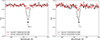 |
Fig. 1. Comparison of the observed spectra from GALAH DR4 for our sample RRL DQ Hya (GALAH 170601002101298) and another RRL with very similar atmospheric parameters and metallicity by D’Orazi et al. (2024). |
Spectroscopic observations of our s-rich RRLs were performed using HERMES@AAT as part of the GALAH survey. Due to the short pulsation period of RRLs, typically less than a day, we chose not to use the survey spectrum because it consists of stacked spectra, leading to total exposure times exceeding one hour. Instead, we retrieved single-exposure spectra from the AAT archive and combined only those with total exposure times of less than 40 minutes. This approach enables us to achieve a minimum signal-to-noise ratio (S/N) of 30 per pixel in the red arm (approximately 6500 Å) for both spectra. Additionally, one of the two stars, DQ Hya, was previously observed with UVES at the VLT, featuring a resolving power of R ≈ 35 000. We selected two spectra, in red and blue, acquired at the pulsation phase around ϕ ≈ 0.5 (see Table 1), and discarded spectra observed at phases near ϕ ∼ 0.8 − 0.9. At these extreme phases, RR Lyrae stars become hotter than 7000 K, making abundance analysis challenging due to the lack of suitable spectral lines. According to For et al. (2011), the optimal phase range for maximising line identification in the spectra of variable RR Lyrae stars is approximately ϕ = 0.3 − 0.4. While the red spectrum (λλ 4800−6800 Å) has a S/N per pixel of approximately 50, the blue spectrum (λλ 3300−4500 Å) has a lower S/N of 23. To our knowledge, no other high-resolution spectra are available for the other sample star (ASAS J153830−6906.4).
Observations used in this work.
Table 1 provides details of our spectroscopic observations. We kept the original archival nomenclature for the names of the spectra to facilitate easy retrieval from the corresponding sources. Alternative names for the stars are listed in Column 2 of the table, along with the S/N, nominal resolutions, Modified Julian Date, phase of the spectra and instantaneous radial velocities. We employed iSpec (Blanco-Cuaresma 2019) to compute the radial velocities (RVs) for each spectrum, using a cross-correlation technique with a synthetic spectrum calculated based on the atmospheric parameters listed in the original GALAH DR4, while accounting for the different instrumental resolutions. Our final RV measurements agree very well with the GALAH values, with a mean difference of less than 0.5 km/s. The same set of synthetic spectra was also used to perform continuum normalisation. As previously done in D’Orazi et al. (2024, 2025), we used the MARCS grids of model atmospheres (Gustafsson et al. 2008) and TSFitPy (Gerber et al. 2023; Storm & Bergemann 2023), the Python wrapper of Turbospectrum v.20 (Plez et al. 2025, and references therein). This allows the computation of Non-Local Thermodynamic Equilibrium (NLTE) synthetic profiles on-the-fly and fast optimisation algorithms.
Effective temperatures (Teff) were determined by fitting the wings of the Hα profiles after masking the central region. We employed three different fitting procedures: fitting the entire profile (from 6550 to 6570 Å) and fitting the left and right wings separately. The measurements from these methods showed good agreement, and we adopted the standard deviation of the three as a conservative estimate of the error in Teff. Surface gravity (log g) was derived using the ionisation balance of neutral and singly ionised lines of Fe and Ti. This approach was chosen due to the limited number of available lines in the GALAH spectra, caused by incomplete spectral coverage across the optical band. Similarly, the microturbulent velocity (Vmic) was obtained by coupling lines of Fe and Ti and adopting the same procedure described in D’Orazi et al. (2024). As this is an iterative process, an initial estimate of the titanium abundance was adopted based on the first-guess measurements of Ca and Mg abundances. The analysis was then repeated iteratively until convergence was achieved between the derived stellar parameters and the Ti abundances. Uncertainties in the surface gravity (log g) were estimated by iteratively adjusting its value until the ionisation equilibrium condition was no longer satisfied within 2.5σ of the measurement uncertainty. For the Vmic values, we adopted a conservative error estimate of 0.5 km s−1.
The line list used is provided in Table A.1 and includes references from the Gaia-ESO line list (Heiter et al. 2021), the VALD database (Ryabchikova et al. 2015), and Lawler et al. (2013) for Ti I lines. From the GALAH spectra, we were able to determine the abundances of certain elements using specific spectral lines: carbon through the C I line at 6587.6 Å, yttrium using Y II at 4883 Å, and barium via the Ba II lines at 5853 and 6496 Å. In contrast, the high-resolution UVES spectra for DQ Hya also allowed us to identify zirconium, lanthanum, cerium, neodymium, and europium, in addition to yttrium and barium (based on a larger set of spectral features). This was possible due to a larger wavelength coverage (see Table A.1 for the complete line list). To further corroborate the kinematic classification of our sample stars as belonging to the thin disc, thick disc, or halo of the Galaxy, we also aimed to estimate their α-element abundances. We derived calcium and magnesium abundances for both stars.
Examples of spectral synthesis computation for the HERMES and UVES spectra of DQ Hya are presented in Figs. A.1 and A.2. Non-Local Thermodynamical Equilibrium (NLTE) abundances were inferred for Fe, Ca, Mg, Ti, Y, Ba, and Eu, while for the remaining species (C, La, Ce, Nd, and Zr), we had to rely on LTE assumptions since departure grids are not available in TSFitPy. As supported by results from Alexeeva & Mashonkina (2015), the C I line at 6587 Å is not significantly affected by NLTE departures; this is also clarified in the caption of Fig. A.2. Moreover, the agreement among the s-process elements–aligning with theoretical expectations due to their common production mechanism–indicates that NLTE effects are likely to be negligible for La, Ce, and Nd. NLTE corrections for Eu, Ba, and Y are within 0.10 dex, roughly matching our typical uncertainties. Due to the large overabundances observed, these corrections do not influence the main conclusions of this study.
There are two types of uncertainties in abundance determinations: one affecting individual spectral lines, which includes random errors in best-fit determination (or equivalent width measurements), oscillator strengths, damping constants, and continuum displacements, and another affecting the entire set of lines, primarily originating from uncertainties in the stellar atmospheric parameters. For the first type, we use the standard deviation of the mean abundance for each species (σ), which is reported as the associated error in Tables 2 and 3. Additionally, we evaluated abundance sensitivities by varying one stellar parameter at a time and assessing the resulting impact on the [X/Fe] ratios; sensitivities for star DQ Hya are given in Table A.3.
Stellar parameters and abundances inferred from the HERMES spectra.
3. Results
Stellar parameters and abundances derived from HERMES spectra for DQ Hya and ASAS J153830−6906.4 are summarised in Table 2. Despite their advanced evolutionary stage (for which C is expected to be depleted by the first dredge-up), both stars display significant enhancements in [C/Fe], approximately ≈ + 0.5 dex. Their α-element abundance patterns are consistent with those of older Galactic populations, such as the thick disc or halo (see Sect. 4.2). Despite having similar metallicities around [Fe/H] ≈ −1, DQ Hya exhibits markedly higher enhancements in the [Y/Fe] and [Ba/Fe] ratios: more than an order of magnitude above solar ([Y/Fe] = 1.20 ± 0.10, [Ba/Fe] = 1.50 ± 0.12). In contrast, ASAS J153830−6906.4 shows more moderate values of [Y/Fe] = +0.33 ± 0.10 and [Ba/Fe] = +0.78 ± 0.06. In both cases, the second-peak s-process element Ba exceeds the first-peak elements, resulting in positive [Ba/Y] ratios. Due to the limited number of heavy element lines accessible from the GALAH spectra, a more detailed analysis of the s-process pattern was performed using the UVES spectra for DQ Hya (see Table 3). Along with Ba and Y, we derived abundances for the first-peak element (Zr), the second-peak elements (La, Ce, and Nd) and the r-process element Eu. Our results confirm a general overabundance of all s-process elements, with higher amounts of second-peak elements (Ba, La, and Ce) than the first-peak elements Y and Zr.
Stellar parameters and additional n-capture element abundances of DQ Hya from UVES spectra.
The [Eu/Fe] ratio also exceeds solar values; however, the observed trend of [Eu/Fe] versus [La/Fe] does not conform to the patterns seen in CEMP-r stars (see e.g. Masseron et al. 2010; Karinkuzhi et al. 2021). In Fig. 2 we display the relation between [La/Fe] and [Eu/Fe] for various metal-poor heavy-element rich stellar populations: CEMP-s stars from Masseron et al. (2010) and Roederer et al. (2014), CEMP-r stars from Masseron et al. (2010), and our enriched RRLs, DQ Hya and TY Gruis, for which Eu abundances could be measured. These results support classifying these stars as s-process-enhanced objects, likely resulting from mass transfer from a former AGB companion.
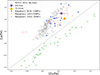 |
Fig. 2. Ratios of [Eu/Fe] vs. [La/Fe] for CEMP-r and CEMP-s stars by Masseron et al. (2010), CEMP-s stars by Roederer et al. (2014), Ba stars by Roriz et al. (2021), and the s-rich RRLs DQ Hya and TY Gruis. The dashed line is the 1:1 relationship. |
As extensively discussed in Cseh et al. (2018, 2022), comparing [hs/ls]3 ratios across different studies is challenging, primarily because different studies often include or exclude certain elements. Crucially, Ba abundances are usually considered unreliable due to the strong and nearly saturated behaviour of the commonly used Ba II lines (e.g. 5853, 6496 Å). Therefore, barium should not be included in the calculation of mean abundances for second-peak s-process elements. Our findings support this approach; in fact, the [Ba/Fe] ratios are systematically higher than those of other second-peak elements such as La and Ce, despite the same nucleosynthetic origin. For this reason, we focus instead on the ratio of two specific elements: yttrium for the first peak and cerium for the second peak, following Cseh et al. (2018, 2022). It is important to note that, in the subsequent discussion, Ba is used as a proxy for Ce for the star ASAS J153830−6906.4. Since we were unable to measure Ce abundances from the HERMES spectrum, we adopt [Ba/Y] as equivalent to [Ce/Y] in our analysis. However, as previously mentioned, because of the saturation of Ba II lines, this ratio is likely somewhat larger than [Ce/Y], with an estimated difference of approximately 0.2 dex. In Fig. 3 we compare the [Ce/Y] ratios as a function of metallicity for the three s-rich RRLs along with recent literature estimates, namely CEMP-s stars from Roederer et al. (2014) and Ba stars from de Castro et al. (2016), Yang et al. (2024), and Vitali et al. (2024). In the metal-poor regime, RRL TY Gruis is located close to the average distribution of CEMP-s stars as reported by Roederer et al. (2014), although it is important to note that these stars exhibit significant scatter. The star shows a moderate enhancement in [Y/Fe] = 0.26 ± 0.05 and substantial enrichment in second-peak s-process elements, with [Ce/Fe] = 1.05 ± 0.15 and a [Ce/Y] ratio of 0.79 ± 0.10. Within this metallicity range ([Fe/H] ≤ −1.5), all the stars tend to exhibit large [Ce/Y] ratios (≳ + 0.5), which confirms the trend towards producing heavier s-process elements at lower metallicities. This behaviour aligns with the well-known characteristic of the s-process reactions, where a higher neutron-to-seed ratio favours the formation of heavier elements over lighter ones (Gallino et al. 1998; Kobayashi et al. 2020, and references therein). DQ Hya and ASAS J153830−6906.4 occupy a pivotal metallicity range, situated between the CEMP-s stars and their higher-metallicity counterparts, i.e. the Ba stars. As observed in both de Castro et al. (2016) and Yang et al. (2024), most of their stars are located at metallicities above [Fe/H] ≈ −0.5. Although based on low number statistics (only six s-rich stars), at around [Fe/H] ≈ −1, the [Ce/Y] ratios vary from slightly over-solar values to significantly enhanced levels, ranging from [Ce/Y] ∼ 0.15 − 0.75. Notably, at nearly any metallicity bin, there is a considerable spread in [Ce/Y] ratios, suggesting that this variation may be intrinsic rather than due to observational uncertainties4. Finally, we include in Fig. 3 the two Ba stars recently fully characterised by Vitali et al. (2024), which reside within the metal-rich regime of the metallicity distribution. This study is particularly significant because, in addition to radial velocity variations confirming their binarity, the authors detected a near-UV excess in the spectral energy distribution (SED) of one of their two sample stars, J04034842+1551272 (see their Fig. 7). To identify similar excesses as potential evidence of a white dwarf (WD) companion, we searched for GALEX NUV (Wright et al. 2010) photometry for our sample stars. This information is available only for DQ Hya, for which the SED was constructed using the VOSA tool5 (Bayo et al. 2008). The comparison with a Kurucz model (Castelli & Kurucz 2003), as shown in Fig. A.3, indicates excellent agreement, with no excess detected in the NUV domain. However, the absence of any near-UV excess does not constitute definitive evidence, particularly given the old age of our RRLs (see Sect. 4.4), where the WD companion may simply be too faint to be detected.
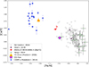 |
Fig. 3. Ratios of [Ce/Y] as a function of metallicity [Fe/H]. |
4. Discussion
4.1. Pulsation properties and absolute magnitude
DQ Hya and ASAS J153830−6906.4 display typical RRab light curves, with some distinct characteristics. DQ Hya, with a period of ≈0.4 days and an amplitude of ≈1.1 G-mag, belongs to the group of HASP (high amplitude short period) RR Lyrae (Fiorentino et al. 2015; Belokurov et al. 2018). ASAS J153830−6906.4 shows a longer period (≈0.6 days) and lower amplitude (≈0.6 G-mag). Despite these differences, the light-curve properties imply similar photometric metallicities, [Fe/H]photo ≈ −1.0 ± 0.36, consistent with the spectroscopic measurements in Table 2. These properties are typical of field RR Lyrae at intermediate metallicity.
From Gaia parallaxes7 and reddening-corrected magnitudes (following Iorio & Belokurov 2021), we obtain MG ≈ 0.7 for ASAS J153830−6906.4 (log L/L⊙ ≈ 1.6) and MG ≈ 0.0 for DQ Hya (log L/L⊙ ≈ 1.9). Applying the parallax offset (≈ − 0.03 mas) from Garofalo et al. (2022) yields MG ≈ 0.9 (log L/L⊙ ≈ 1.5) and MG ≈ 0.2 (log L/L⊙ ≈ 1.8), respectively.
Such a large difference is unexpected given the existence of a theoretical and empirical MG–[Fe/H] relations in the optical bands (see e.g. Marconi et al. 2022; Garofalo et al. 2022). In particular, from the Garofalo et al. (2022) relation calibrated on Gaia DR3 RR Lyrae, we would expect MG ≈ 0.7 for both stars. For ASAS J153830−6906.4, the difference with respect to this prediction is modest and within the combined formal and systematic uncertainties (≈0.2 mag), but for DQ Hya the discrepancy is significant. Two scenarios are possible: (1) DQ Hya is a genuine outlier in the MG–[Fe/H] relation, potentially indicating evolutionary effects (HB stars increases their luminosity evolving towards the AGB phase), peculiar properties or a distinct formation channel (see e.g. Marconi et al. 2018, and Sect. 4.4) or (2) the Gaia parallax is biased, possibly due to blending or unresolved binarity (Sect. 4.5). In the latter case, adopting the empirical MG–[Fe/H] relation of Garofalo et al. (2022), we obtain a distance from the Sun d ≈ 2.9 kpc (in agreement with the distance obtained from the MIR P–L relationship), compared to d ≈ 4.3 kpc from parallax inversion (or d ≈ 3.8 kpc with the offset). In Fig. 8 we show the Kiel diagram for our 2 sample s-rich RRLs along with the PARSEC evolutionary tracks (Chen et al. 2015) and the instability strip location from Marconi et al. (2015).
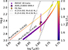 |
Fig. 8. Kiel diagram comparing the RR Lyrae stars analysed in this work (DQ Hya shown as a diamond, ASAS J153830−6906.4 as a square) with horizontal branch evolutionary tracks from the PARSEC V1.2S database (Chen et al. 2015, circles; masses and metallicities are indicated in the plot). The colour map represents the bolometric luminosity. For the observed stars, luminosities are derived using distances from parallaxes (see Sect. 4.1). The size of the circles along the tracks provides a qualitative indication of the time spent in each region of the diagram, with the largest symbols corresponding to approximately ten times longer evolutionary timescales than the smallest ones. The grey lines indicate the instability strip from Marconi et al. (2015), assuming a metallicity of Z = 0.002 and stellar masses of 0.56 M⊙ (dotted line) and 0.62 M⊙ (dashed line). The comparison is purely qualitative and does not represent the result of a fit. |
4.2. Kinematics and chemodynamics
To infer the kinematic properties of the two stars, we use their Gaia DR3 astrometric data (parallax, proper motions, and radial velocity) to initialise orbit integrations in the Milky Way, adopting two models for the Galactic potential: that of McMillan (2017, M17) and Allen & Santillan (1991, AS91). For the orbit integration, we use the leapfrog integrator implemented in the orbit module of the PYTHON package GALPY (Bovy 2015)8. All the orbits are integrated forward for 1.5 Gyr. To transform the observed quantities into six-dimensional phase-space coordinates in the Galactic reference frame, we use the PYTHON module ASTROPY9 (Astropy Collaboration 2013, 2018, 2022). For the M17 potential, we adopt a solar position of R⊙ = 8.21 kpc and a circular velocity at the solar radius of Vlsr = 233.1 km s−1; for AS91, we use R⊙ = 8.5 kpc and Vlsr = 220 km s−1. In both cases, we assume that the Sun is located 20.8 pc above the Galactic midplane (Bennett & Bovy 2019). The Sun’s peculiar motion with respect to the local standard of rest (LSR) is taken as (U⊙, V⊙, W⊙) = (11.1 ± 1.3, 12.2 ± 2.1, 7.25 ± 0.6) km s−1 (Schönrich et al. 2010), where the right-handed Cartesian Galactic coordinate system is defined such that U points towards the Galactic centre, V in the direction of Galactic rotation, and W towards the North Galactic Pole.
We estimate the distances of the two stars from the Sun by inverting their parallaxes, an approach justified by their small relative parallax uncertainties (less than 10%). In the case of DQ Hya, however, the discrepancy between the parallax-based distance and the one expected from its absolute magnitude given its metallicity suggests a possible bias in the parallax measurement (see Sect. 4.1). Therefore, for this star, we repeat the orbit integration using the distance inferred from the magnitude–metallicity relation for field RR Lyrae stars (Garofalo et al. 2022). To account for uncertainties, in addition to the orbit computed using the fiducial parameters, we integrate 105 additional orbits by sampling the posterior distribution of the astrometric parameters. We assume normally distributed errors and take into account both the uncertainties and covariances reported in the Gaia DR3 catalogue. Additionally, we sample the values of the Sun’s peculiar motion by considering the errors reported in Schönrich et al. (2010). We also repeat the orbit integrations by applying the parallax offset estimated for field RR Lyrae stars by Garofalo et al. (2022, approximately −0.03 mas), as well as the offset determined as a function of magnitude, colour, and position by Lindegren et al. (2021, approximately −0.04 mas for DQ Hya and −0.03 ASAS J153830−6906.4). The results of the orbit integrations are consistent with those obtained without applying any parallax correction; therefore, we do not discuss them further in the rest of the paper.
Figure 4 shows the fiducial orbits of the two stars in the Galactic R − z plane, and Fig. 5 shows the joint posterior distribution of the orbit eccentricity and the maximum vertical displacement reached by the orbits; additional properties are summarised in Table A.4. As illustrated in Fig. 4, the orbits computed under the two Galactic potentials are very similar. Therefore, we discuss them in general terms without focusing on the details of each specific model. The two stars exhibit tube-like orbits typical of stars belonging to the Galactic disc. DQ Hya has a low eccentricity (≈0.1), but a significant vertical excursion (zmax > 1 kpc), instead ASAS J153830−6906.4 remains close to the disc (zmax < 0.5 kpc) but exhibits higher eccentricity (≈0.25) with notable radial excursion bringing it in the inner part of the Galaxy (R ⪅ 5 kpc). These orbital properties put the stars in an intermediate regime between the thick disc stars and the hottest (and likely oldest) thin disc stars. Indeed, Fig. 5 shows that when compared with the disc stellar catalogue by Bensby et al. (2014), ASAS J153830−6906.4 occupies the regions of stars classified as in-between the likely thin and thick disc stars. DQ Hya seems to be more consistent with the thick disc component, especially considering the orbit in which the distance is estimated from the parallax. To obtain a more quantitative estimate of the thin or thic disc membership likelihood, we adopt a method similar to that of Bensby et al. (2014), but using the thin and thick disc Galactic components as defined by Robin et al. (2003). The membership likelihood for each Galactic component is
![Mathematical equation: $$ \begin{aligned} p_i =\frac{\rho _i(\boldsymbol{x}) \times \mathcal{N} (\boldsymbol{v}|\boldsymbol{\theta }_{\mathrm{kin},i}) \times \mathcal{N} (\mathrm{[Fe/H]}| \boldsymbol{\theta }_{\mathrm{[Fe/H]},i})}{\sum ^{N_{\rm components}}_i p_i}, \end{aligned} $$](/articles/aa/full_html/2025/12/aa57188-25/aa57188-25-eq1.gif) (1)
(1)
where ρ is the local volumetric density of the Galactic component at the position of the star (Table 3 in Robin et al. 2003). The second term is a multivariate normal distribution, where θkin refers to the kinematic properties of the component (velocity dispersion and asymmetric drift, as given in Table 4 of Robin et al. 2003). The third term is a normal distribution in metallicity, with θ[Fe/H] denoting the mean and standard deviation of the metallicity distribution of the given component as reported in Table 2 of Robin et al. (2003). The main difference with respect to the membership analysis performed by Bensby et al. (2014) is that we include metallicity in the likelihood computation. The likelihood is evaluated for all 105 orbit realisations, and we also sample 105 values of the stellar metallicity, assuming Gaussian uncertainties based on the values reported in Table 2.
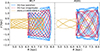 |
Fig. 4. Integrated orbits of DQ Hya (thick solid line: distance from parallax inversion; dashed line: distance estimated from the RR Lyrae magnitude–metallicity relation) and ASAS J153830–6906.4 (thin solid line: distance from parallax inversion), computed using the Milky Way potential models by McMillan (2017, M17, left panel) and Allen & Santillan (1991, AS91, right panel). |
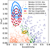 |
Fig. 5. Comparison of the orbital properties, eccentricity, and maximum distance from the Galactic plane, of DQ Hya and ASAS J153830−6906.4 with the sample of disc stars from Bensby et al. (2014, B14). The contours represent the 68%, 95%, and 99.7% confidence intervals from 105 orbit realisations; line styles and colours follow those used in Fig. 4. Circle and square markers indicate stars classified by B14 as likely thin disc and thick disc members, respectively, based on a thick-to-thin disc likelihood ratio of < 0.5 and > 2. Star-shaped markers represent stars in between the two components with intermediate likelihood ratios. Both our orbit integrations and those in B14 adopt the Galactic potential from Allen & Santillan (1991). |
The results of the membership analysis are reported in Table A.4. If the metallicity term in Eq. (1) is neglected, the results are consistent with the qualitative comparison shown in Fig. 5, suggesting an ambiguous classification between the thick disc and the older components of the thin disc. However, once metallicity is included, the membership probability strongly favours an association with the thick disc (pthick > 0.9) for both stars, regardless of the assumed distance for DQ Hya or the Galactic dynamical model used. Notably, both stars exhibit enhancement in α-elements (Ca, Mg, and Ti), confirming their likely affiliation with the thick disc. This demonstrates that combining kinematic and detailed chemical information is essential; studies relying solely on dynamical parameters without considering elemental abundances can lead to misleading conclusions. We plan to further explore this point in a forthcoming publication.
4.3. Comparison with AGB models
In Fig. 6 we present a comparison of the [Ce/Y] ratios as a function of metallicity for our RR Lyrae stars, as well as Ba and CEMP-s stars, alongside AGB models from the FRUITY and Monash groups. The FRUITY models (Cristallo et al. 2009, 2011, 2015, 2016) considered in this study were obtained from their database10 using the standard 13C pocket and not including rotation. The Monash models are based on previous studies by Lugaro et al. (2012), Fishlock et al. (2014), Karakas & Lugaro (2016), Karakas et al. (2018). We refer the reader to Käppeler et al. (2011), Karakas & Lattanzio (2014), and Lugaro et al. (2023) for a more detailed discussion on the models and nucleosynthesis of AGB stars.
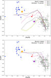 |
Fig. 6. Comparison of observations with stellar models by FRUITY (Cristallo et al. 2011) and Monash groups (Karakas et al. 2018, and references therein). Symbols are the same as in Fig. 3. Masses are in M⊙. |
In our analysis, we focused on AGB models with masses ranging from 1.5 to 5 M⊙, ensuring they meet the criteria of including third dredge-up episodes while avoiding efficient hot bottom burning (HBB), which would destroy carbon. In the low-mass models (below ≈4 M⊙, depending on the metallicity) the 13C(α,n)16O reaction is activated and dominates the neutron production for the s-process in a so-called 13C pocket. We note that the larger mass (5 M⊙ and above) FRUITY models at low metallicities experience hot bottom burning and hot-third dredge up simultaneously, which prevent the formation of 13C neutron sources (Cristallo et al. 2015).
The previously published Monash grid lacked data for metallicity [Fe/H] = −1.2, including a 13C pocket above 3 M⊙. Consequently, we calculated new models at Z = 0.001 ([Fe/H] = −1.2) for 4.5 M⊙. using the same methods and procedures outlined in Karakas & Lugaro (2016), where we evolve the 4.5 M⊙ model from the main sequence to the end of the thermally pulsing AGB phase. We note that the 4.5 M⊙ does have some HBB, but it is relatively mild and the model remains carbon rich. For the evolutionary sequences, we used the same mass-loss rate on the AGB as described in Karakas et al. (2018), which assumes Bloecker (1995) with η = 0.01, including the same input physics as described in that paper. The AGB model experienced 30 thermal pulses, where 29 had efficient third dredge-up. Note that the model of the same mass and metallicity from Fishlock et al. (2014) experienced 79 thermal pulses, owing to the use of Vassiliadis & Wood (1993) mass-loss on the AGB instead. Our new model also experienced hot bottom burning, with a peak temperature of around 80 million K. Post-processing nucleosynthesis calculations were performed to obtain the s-process element abundance predictions, where we include a 13C pocket via the same method as outlined in Karakas & Lugaro (2016), where the mass of the partially mixing zone of protons was set at Mpmz = 1 × 10⁻⁴ M⊙. In the further discussion, we use the new 4.5 M⊙ Monash model instead of the 4 and 5 M⊙ models without a 13C pocket. This allows us to compare the observational data only to Monash models that were calculated with the inclusion of a 13C pocket along the metallicity range of the stars of interest in this study.
Comparing the different Monash and FRUITY models across the metallicity range, the models generally reproduce the observations well at higher metallicities ([Fe/H] ≳ −0.5), where most Ba stars are located. In particular, they capture the expected and observationally confirmed declining trend of [Ce/Y] ratios with increasing metallicity, which has been extensively discussed in previous studies (Cseh et al. 2018, 2022; Roriz et al. 2021). Overall, the models perform adequately at high metallicity. However, neither set of models can explain the elevated [Ce/Y] ratios observed in CEMP-s and TY Gruis stars. At metallicities below −2, the models underestimate the ratios for any given AGB mass. Although a comprehensive examination of the different model sets is beyond the scope of this paper, we also checked the rotating models. We found that they do not adequately explain the patterns observed at low metallicities. Further investigations will be necessary.
As shown in Fig. 6, our two RR Lyrae stars are positioned in the intermediate range of the metallicity distribution, i.e. [Fe/H] ≈ −1. Based on the model predictions, the FRUITY grids for masses between 1.5 and 4 M⊙ can reproduce the observed distribution, once the dilution of AGB material is taken into account. Similarly, Monash models for 1.5, 2.0, and 4.5 M⊙ can all explain the observed abundance patterns in the [Ce/Y] versus [Fe/H] plane, again assuming that dilution effects are considered (see following discussion). Following Cseh et al. (2022), we calculated the dilution factors (which take into account the mass transfer and the mixing) of AGB abundances using the relationship
![Mathematical equation: $$ \begin{aligned} \mathrm{[X/Fe]}_{\rm dil} = \log (10^\mathrm{[X/Fe]_{\rm ini}} \times (1 - \delta ) + 10^\mathrm{[X/Fe]_{\rm AGB}} \times \delta ), \end{aligned} $$](/articles/aa/full_html/2025/12/aa57188-25/aa57188-25-eq2.gif) (2)
(2)
where [X/Fe]ini represents the initial abundances in the models, assumed to be solar for all species; [X/Fe]AGB gives the final abundances produced by the AGB; and [X/Fe]dil is the abundance measured in our RRLs DQ Hya and TY Gruis. We omit ASAS J153830−6906.4 in this context due to uncertainties related to its barium abundance, which we use as a proxy for Ce; this element was not measured in the HERMES spectra.
We then calculated the δ value, defined as 1/dil, which represents the ratio between the total mass, i.e. the original envelope mass of the Ba star plus the mass transferred from the AGB star to its companion, and the transferred AGB material, and thus dil = Mtotal/MAGB, trans = (MBa, env + MAGB, trans)/MAGB, trans (see Cseh et al. 2022 and references therein). Thus, a value of δ = 0 corresponds to no mass transfer from the AGB star, and a value of δ = 1 represents the unrealistic case of no mixing of the AGB material into the RRL star after the mass transfer. Typical values reported in Cseh et al. (2022) and Yang et al. (2024) are δ = 0.3; however, in some cases, larger values can be derived (see discussion in the corresponding papers). We constrained the dilution factors using both [Ce/Fe] and [Y/Fe] abundances, with the expectation that they should yield consistent δ values. However, this is not the case for most of our calculations, so caution is advised when interpreting these dilution factors. In particular, for the metal-poor TY Gruis, the [Y/Fe] ratio results in δ values typically ranging from 0.02 to 0.1 for both Monash and FRUITY models across nearly all stellar masses. This is expected, given the low metallicity of the star, where even a small amount of transferred mass can significantly alter the surface abundances of the companion. However, the FRUITY models do not produce sufficient Ce (as previously noted and clearly shown in Fig. 6); therefore, when calculating the same dilution factor using [Ce/Fe] abundances, we obtain δ values for masses of 1.5 and 2 M⊙ that are a factor of 3 higher than those derived from [Y/Fe], while yielding unrealistic dilution values for masses of 3 M⊙ and above. Conversely, the Monash models tend to converge towards similar δ values for masses between 1.5 and 3 M⊙; for masses between 4 and 5 M⊙, the production of Ce becomes very limited and unphysical δ values of larger than 0.7 would be required. For DQ Hya, the FRUITY models would require δ values greater than 1 across all masses for Y, while [Ce/Fe] abundances would require δ values of 0.48, 0.25, and 0.58 for 1.5, 2.0, and 3.0 M⊙, respectively. In contrast, the Monash models suggest δ of 0.82, 0.37, and 0.86 for the [Y/Fe] ratios at masses of 1.5, 2.0, and 3.0 M⊙, respectively. However, for [Ce/Fe] ratios, the δ values are estimated at 0.26, 0.09, and 0.24 for 1.5, 2.0, and 3.0 M⊙, while higher masses imply unrealistically large δ values exceeding 1, indicating these more massive AGB stars do not produce enough Ce, consistent with a decreasing TDU efficiency and smaller 13C pocket.
Due to the substantial discrepancies observed in the calculated dilution factors, we are unable to definitively determine the mass of the AGB companion at this time; additional studies are required. Still, some limits on the amount of accreted material can be inferred by noting that DQ Hya and the other two s-rich RRLs will pass through the instability strip while helium is burning in their core, as RR Lyrae stars. Its pulsation and evolutionary characteristics can thus provide constraints on the possible accreted mass. We discuss this in more detail in Sect. 4.4.
4.4. Formation scenarios
For many years, RR Lyrae stars were considered reliable tracers of old stellar populations due to their predominant presence in the Galactic halo, globular clusters, and generally in ancient stellar systems. However, this paradigm has been challenged by the discovery of metal-rich RR Lyrae stars exhibiting thin disc kinematics and low α-element abundances (Layden 1995; Chadid et al. 2017; Prudil et al. 2020; Crestani et al. 2021; Iorio & Belokurov 2021; Gozha et al. 2021, 2024; D’Orazi et al. 2024, and references therein). There is an ongoing debate in the literature regarding the formation channels of metal-rich RR Lyrae stars (see summary in Zhang et al. 2025). The current hypotheses include single-star evolutionary pathways, possibly involving extragalactic origins to account for their peculiar chemical signatures (Gozha et al. 2021, 2024; D’Orazi et al. 2024), and binary formation scenarios (Bobrick et al. 2024). In the latter case, material transfer may occur via mechanisms such as accretion through a circumbinary disc. Our two RR Lyrae stars exhibiting s-process enrichment, occupy a parameter space in metallicity ([Fe/H] ≈ −1) where single-stellar evolutionary models typically predict their existence. Nevertheless, several intriguing hypotheses warrant further consideration. Comparisons with AGB models suggest that the RR Lyrae progenitors may have accreted material from an approximately ≈1.5−5.0 M⊙ AGB companion. Considering the rapid evolutionary timescales of more massive stars, this indicates that mass transfer likely occurred while the secondary star (the current RR Lyrae) was still on the main sequence.
Comparing the luminosity (Sect. 4.1), the spectroscopic temperature, and the log g measurements (Table 2) with PARSEC tracks (Nguyen et al. 2022), the star ASAS J153830−6906.4 is consistent with an HB star of about 0.65 M⊙, located close to the ZAHB. A similar result is obtained for DQ Hya if its luminosity is assumed to follow the MG–[Fe/H] relation for field RR Lyrae stars (Garofalo et al. 2022). In contrast, adopting the higher luminosity inferred from the parallax-based distance (log L/L⊙ > 1.8; see Sect. 4.1), DQ Hya is instead consistent with a late evolutionary phase of an HB star of about 0.58−0.60 M⊙. Assuming a typical RGB mass loss of about 0.20−0.25 M⊙ at the metallicity of the RR Lyrae (Gratton et al. 2010; Tailo et al. 2021), the progenitor mass at the onset of the red giant branch would be in the range 0.8−0.9 M⊙. Under this scenario, assuming a typical δ of 0.3 (Cseh et al. 2022), which translates to a dilution factor of roughly 3, approximately 0.1 M⊙ would have been accreted. This aligns with standard accretion models depicted for Ba giant stars. However, due to the significant uncertainty in dilution factors, we avoid making any definitive conclusions at this point. Moreover, the scenario assumes that after the initial pollution event, no further binary interactions occurred.
Another plausible scenario involves a second episode of mass transfer occurring as the RR Lyrae progenitor ascends the red giant branch for the first time. In this case, the resulting RR Lyrae could be classified as a binary-produced RR Lyrae, as discussed by Bobrick et al. (2024), but with the key difference that it experienced two distinct mass transfer events. The first occurred when the star was on the main sequence, accreting material from an AGB companion and producing the observed chemical anomalies. The second transfer happened later during its RGB phase, where the star, now a giant, transferred some of the previously accreted material back, potentially to the current white dwarf companion. If this scenario holds, the second mass transfer could impose constraints on the current properties of the binary system. Following Bobrick et al. (2024), for the RR Lyrae progenitor to interact with its white dwarf companion, the initial orbital period would need to be shorter than approximately 700 days. After this interaction, the system’s orbital period would likely be on the order of 1000 days. In addition, within this scenario the mass lost during the RGB is significantly larger (⪆0.4 M⊙) than expected from single stellar evolution, implying more massive progenitors for the RR Lyrae stars.
An additional scenario is that the current RR Lyrae are a member of the sub-luminous post-AGB/post-RGB family crossing the instability strip (see e.g. Oomen et al. 2018). Indeed, using Gaia DR3, Oudmaijer et al. (2022) showed that a subgroup of stars previously classified as post-AGBs were too sub-luminous for the expected post-AGB evolution (≳102 L⊙) and more likely post-RGBs, descendants of RGB interactions. Without speculating about the origin of these sub-luminous post-AGB-like systems, we note that the current RR Lyrae have surface temperatures, luminosities and abundances indeed consistent with this population, thus suggesting a shared origin. Partially supporting this interpretation is that DQ Hya seems to have a slightly higher absolute magnitude than other field RR Lyrae with a similar metallicity (see Sect. 4.1), although the ASAS star is consistent in temperature and luminosity with the regular RR Lyrae in globular cluster M4. It may also be worth noting that one of the few RRLs confirmed to be in a binary system is a post-RGB star, a star whose envelope was stripped during the RGB phase and is now crossing the instability strip (Pietrzyński et al. 2012). We also note that several other sub-luminous post-AGB-like stars from Oudmaijer et al. (2022) are also located in the luminosity–temperature region surrounding the RRL instability strip (1 < log L/L⊙ < 2, 3.7 < log T/K < 3.9). We compared the Hertzsprung-Russell diagram positions of these stars with the theoretical RR Lyrae IS boundaries computed by Marconi et al. (2015), and then searched for light curves among the observations of the TESS (Transiting Exoplanet Survey Satellite, Ricker et al. 2015) mission. TESS can detect RR Lyrae stars over a wide brightness range and even in crowded fields with high fidelity (Molnár et al. 2022). Four out of the five stars within or near the IS boundaries do not show any large-amplitude pulsations that would resemble an RR Lyrae star. The fifth target has not been observed by TESS yet, but it was not detected as a variable by the Gaia mission, which strongly suggests that it is not pulsating as an RR Lyrae either (Gaia Collaboration 2023; Clementini et al. 2023). Additionally, observations of post-AGB stars are often associated with infrared excesses resulting from the recently stripped material (see e.g. Dell’Agli et al. 2023). However, neither of the two RR Lyrae stars examined in this work exhibits any signs of such excess (see the WISE photometry for DQ Hya shown in Fig. A.3). Therefore, the association of the current RR Lyrae with this population should be examined carefully before drawing any conclusions.
Overall, none of the scenarios discussed above can be confirmed as the definitive formation pathway for these two RR Lyrae stars. In particular, if DQ Hya is truly an evolved RR Lyrae, this raises an important point to consider. The time spent by an HB star of initial mass 0.58 M⊙ in the instability strip is more than two orders of magnitude shorter than that of a canonical RR Lyrae at the same metallicity. Simple statistical reasoning therefore implies that it is already rare to find such an object in a sample of ≈500 RR Lyrae analysed in this work. It is even more unlikely to encounter it within the subsample of only two stars showing peculiar abundances, unless the high luminosity of DQ Hya and its chemical peculiarity are connected through a distinct formation channel.
Future works will need detailed binary evolution modelling, specifically tailored to the metallicity, masses, and orbital parameters relevant to these systems. This will include considerations of multiple mass transfer episodes, angular momentum loss, and surface abundance evolution. Such work will be presented in a dedicated upcoming paper.
4.5. Search for binary signatures
Since Ba stars are known to be members of binary systems, their orbital parameters can often be constrained through RV observations (Jorissen et al. 2019; Escorza et al. 2019). The RV variations over time provide direct evidence of binarity and allow for the determination of orbital periods, eccentricities, and mass functions. However, for RR Lyrae stars, measuring RVs is significantly more challenging. This difficulty arises from their large-amplitude pulsations, which cause substantial and periodic changes in their spectral lines that can complicate the detection of orbital-induced RV variations. Consequently, traditional spectroscopic methods are less effective for these variables. As an alternative approach, we can utilise astrometric data from Gaia to search for signatures of binarity. Gaia’s precise measurements of parallaxes and proper motions can reveal orbital motions on the sky, even when RV data are unavailable or inconclusive.
Additionally, the coherent pulsations of RR Lyrae stars themselves can be exploited to infer orbital parameters from photometry alone. This method involves analysing the light-time effect – the slight shifts in pulsation arrival times caused by the star’s orbital motion around a common centre of mass. By carefully monitoring the periodic variations in pulsation timings, it is possible to detect the presence of a companion and estimate orbital elements, even without spectroscopic data.
Unfortunately for RR Lyrae stars, the Blazhko effect, the quasi-periodic modulation of the pulsation amplitude and phase, can mask any O–C signal caused by the light-time effect (Benkő et al. 2014). Furthermore, many RR Lyrae stars show O–C curves that are characterised by largely unexplained rapid changes and sudden breaks, although others show clear secular period changes (see e.g. Le Borgne et al. 2007). However, the feasibility of the light-time method for non-Blazhko RR Lyrae stars was proven by Hajdu et al. (2015, 2021), who identified several RR Lyrae binary candidates. O–C curves of the stars can thus reveal both the presence and distance of a companion and/or the rate and direction of the variable’s evolution across the instability strip, thereby helping to constrain different evolutionary scenarios. This work will be presented in a dedicated publication.
4.6. Astrometric signature
Unresolved binary systems can be detected through precise astrometric measurements, as the orbital motion of the photocentre causes systematic deviations from the behaviour of a single star. Gaia DR3 has provided the first catalogue of astrometric binaries (Halbwachs et al. 2023; Holl et al. 2023). However, neither of the two RRLs analysed in this work is flagged as an astrometric binary in Gaia DR3. However, this does not rule out the presence of companions, as Gaia’s astrometric binary detection is not sensitive to all orbital configurations (El-Badry et al. 2024). In addition, in Gaia DR3 no binaries solution are reported for binary periods Porb < 20 000 δϖ/ϖ days (ϖ/δϖ is the parallax over its error), corresponding to Porb ⪅ 1700 days for DQ Hya (ϖ/δϖ≈12) and Porb ⪅ 800 days for ASAS J153839−6906.4 (ϖ/δϖ≈26). Moreover, Gaia DR3 has detected very few astrometric binaries beyond roughly 2 kpc, and since both stars in this study are located at distances greater than that, their intrinsic likelihood of being detected as binaries by Gaia’s current pipeline is relatively low.
Another commonly used diagnostic is the Renormalised Unit Weight Error (RUWE), which provides a normalised assessment of how well Gaia’s astrometric data fit a single-star model (similar in concept to a reduced χ2). Solutions for well-behaved, single sources typically have RUWE values close to 1, while higher values suggest a poorer fit to the single-star assumption. Elevated RUWE can result from crowding, background contamination, or intrinsic variability. One of the main causes is unmodelled binarity, where the orbital motion of the photocentre is not properly accounted for (Belokurov et al. 2020; Penoyre et al. 2022; Castro-Ginard et al. 2024). A RUWE threshold of 1.4 is often adopted to distinguish between reliable and potentially biased astrometric solutions (Halbwachs et al. 2023). For our targets, we find RUWE = 1.27 for ASAS J153839−6906.4 and RUWE = 1.72 for DQ Hya. The first value lies within the typical range for single stars, while the second exceeds the 1.4 threshold, suggesting a possible bias in the astrometric fit and raising the possibility of an unresolved companion. DQ Hya also shows a significant difference between the distance estimate with parallax and that from the magnitude-metallicity relation (see Sect. 4.1), supporting the scenario in which the parallax estimate is biased by the presence of a companion. However, the significance of the RUWE can be affected by photometric properties and sky position (Castro-Ginard et al. 2024). Variability can also influence the RUWE distribution: Belokurov et al. (2020) found that, for the Gaia DR2 RR Lyrae sample, the median RUWE depends systematically on pulsation properties and apparent magnitude. Therefore, to assess the significance of the measured RUWE values for our targets, we compare them against two control samples:
-
Sky control sample: All Gaia DR3 sources within 1° of the analysed RR Lyrae stars, with G-band magnitude within 0.5 mag and Gaia colour within 0.1 mag of the target. We also define a subset of the control sample in which we remove all the stars classified as astrometric non-single stars in Gaia DR3.
-
RR Lyrae control sample. All Gaia DR3 RR Lyrae variables with light-curve properties similar to the two analysed RR Lyrae stars: periods within 0.15 days, G-band peak-to-peak amplitudes within 0.15 mag, ϕ31 light-curve parameter angles11 within 0.2 rad, and the same magnitude and colour cuts as for the sky control sample.
Figure 7 shows the comparison between the RUWE values of the two analysed RR Lyrae stars and those of the control samples. For ASAS J153830−6906.4, the RUWE lies well within the typical distribution for both the Sky and RR Lyrae control samples. In contrast, DQ Hya is located closer to the tail of the distribution for the Sky control sample, particularly when considering the version cleaned of sources classified as non-single in Gaia DR3. However, even in this case, the RUWE value remains within the 95% confidence interval of the distribution. The comparison with the RR Lyrae control sample instead shows that the DQ Hya RUWE is typical of RR Lyrae stars with similar light-curve properties, i.e. with short periods (≈0.5 days) and large amplitudes (⪆1 mag in the G band), which tend to exhibit higher RUWE values, as discussed in Belokurov et al. (2020).
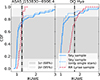 |
Fig. 7. RUWE values (vertical dash–dot black lines) of the two analysed RR Lyrae stars (left: ASAS J153830−6906.4, right: DQ Hya) compared to the cumulative distribution functions of the corresponding control samples. The solid blue line shows the CDF for the sky-position control sample, which includes stars in the same sky area with similar photometry. The dotted blue line shows the CDF for the same sample after removing stars classified as non-single in Gaia DR3. The dashed red line shows the CDF for the RR Lyrae control sample from Gaia DR3, selected to have similar photometry and light-curve properties to the targets (see text for details). The shaded regions indicate the central 68% (dark shading) and 95% (light shading) intervals of the distributions. |
In conclusion, while the RUWE values are somewhat higher than average, they are not indicative of a significant bias in the astrometric fit that would suggest the presence of a binary. This alone cannot exclude an undetected binary companion, but it does help to constrain the possible orbital period: the sensitivity of RUWE to binarity peaks for periods of ∼3 years and decreases rapidly, becoming negligible for periods longer than ∼30 − 50 years (Penoyre et al. 2022; Castro-Ginard et al. 2024).
An additional consequence of this analysis is that we can consider the Gaia DR3 astrometric solutions to be robust for both stars. In particular, this supports the conclusion that DQ Hya is intrinsically brighter than typical RR Lyrae stars of similar metallicity in the field (see Sect. 4.1).
5. Concluding remarks
In this work, we have discovered and analysed two new RR Lyrae stars that exhibit significant s-process element enrichment; this has expanded this rare class of objects (2 in 470 of our sample) beyond the previously known TY Gruis (Preston et al. 2006). Based on detailed elemental abundance analyses, we suggest that these stars may have experienced mass transfer from former AGB companions, which supports their classification as post-mass transfer systems. However, several uncertainties persist. The precise properties of the putative AGB companions, such as their mass and the extent of accreted material, are still unconstrained by model limitations and uncertainties in dilution factors. Different formation scenarios, including mass transfer during the main sequence, second mass transfer episodes on the red giant branch, or the possibility of a sub-luminous post-AGB-like crossing the instability strip, offer plausible explanations but lack definitive confirmation. Our investigation highlights the importance of combining chemical, dynamical, and astrometric data to understand these complex objects.
Although Gaia’s current data do not provide conclusive evidence of binarity for these stars, partly due to observational limitations at their distances, their RUWE values and the consistency with chemodynamical expectations suggest that undetected companions cannot be entirely ruled out. Pulsations can also be used to detect binarity. We searched for time series photometry of both targets in various public databases and in the observations of the TESS (Transiting Exoplanets Survey Satellite, Ricker et al. 2015) mission. Unfortunately, ASAS J153830−6906.4 turned out to be a known Blazhko star (Szczygieł & Fabrycky 2007; Skarka 2013). DQ Hya, however, appears to be a pure fundamental-mode pulsator based on its TESS light curves, and thus amenable to such analysis. A detailed investigation of the O–C curve will be published separately.
Future dedicated binary evolution modelling, along with continued monitoring of orbital and pulsation timing variations, will be essential to elucidate the formation pathways of these intriguing RR Lyrae stars. These efforts will be addressed in upcoming work with the aim of deepening our understanding of stellar evolution and binary interactions of variable stars.
Neutron-capture elements up to bismuth (Z = 83) can be synthesised in various amounts by both the r- and s-processes, while heavier elements are purely r-process products. Also, the production of some elements is so dominated by either the r-process (e.g. Eu, Gd, Dy, and Pt) or the s-process (e.g. Sr, Y, Zr, Ba, La, and Ce) that they are commonly referred to as r- or s-process elements. We follow that convention in this paper. Moreover, alongside the s- and r- neutron capture processes, an intermediate neutron capture process (i-process) is thought to exist (Hampel et al. 2019; Choplin et al. 2022), but it is not addressed here.
The s-process elements, formed via neutron capture in stars, are mainly concentrated in two peaks on the periodic table: the first at neutron magic number N = 50, which includes elements such as Sr, Y, and Zr, and the second at N = 82, comprising elements like Ba, La, Ce, Pr, and Nd (see e.g. Lugaro et al. 2012 and references therein). Elements in the first peak are commonly referred to as light s-process elements (ls), while those in the second peak, such as Ba, La, and Ce, are classified as heavy s-process elements (hs).
The ratio between second-peak heavy (hs) and first-peak light (ls) s-process elements is routinely indicated as [hs/ls].
We note that there is an offset between the [Ce/Y] ratios reported by de Castro et al. (2016) and Yang et al. (2024), with the former tending to show higher [Ce/Y] at similar metallicities. The origin of this discrepancy remains unclear, especially as the Yang et al. sample appears to be at slightly higher metallicities. However, exploring this difference is beyond the scope of this paper, as it is not directly relevant to our focus on the lower metallicity RRLs.
We derived this value using the empirical relation in Iorio & Belokurov (2021); similar values are obtained with the relations in Dékány & Grebel (2022) and Li et al. (2023).
Given the high parallax-over-error ratio for both stars (> 10), distances are estimated by simple inversion.
http://github.com/jobovy/galpy, we used version 1.11.0. For the M17 potential, we use the built-in model MCMILLAN17, while for AS91 we implement a custom potential module based on the built-in IRRGANG13I model, which shares the same dynamical components as AS91.
https://github.com/astropy/astropy, we used the version 7.1.0.
The ϕ31 is a Fourier phase parameter derived from the decomposition of the light curve; see Clementini et al. (2023).
Acknowledgments
We thank the reviewer for their valuable comments and suggestions that improved the quality of this manuscript. GI thanks Pau Ramos for fruitful discussions on the kinematic association with Galactic components. Part of this work was supported by the Fulbright Visiting Research Scholar program 2024-2025. GI was supported by a fellowship grant from la Caixa Foundation (ID 100010434). The fellowship code is LCF/BQ/PI24/12040020. This research was supported by the ‘SeismoLab’ KKP-137523 Élvonal grant of the Hungarian Research, Development and Innovation Office (NKFIH), by the NKFIH excellence grant TKP2021-NKTA-64 and by the LP2025-14/2025 and LP2023-10 Lendület grants of the Hungarian Academy of Sciences. A.B. acknowledges support from the Australian Research Council (ARC) Centre of Excellence for Gravitational Wave Discovery (OzGrav), through project number CE230100016. SWC acknowledges federal funding from the Australian Research Council through a Future Fellowship (FT160100046) and Discovery Projects (DP190102431 and DP210101299). This research made use of NASA’s Astrophysics Data System Bibliographic Services, as well as of the SIMBAD and VizieR databases operated at CDS, Strasbourg, France.
References
- Abate, C., Pols, O. R., Karakas, A. I., & Izzard, R. G. 2015, A&A, 576, A118 [NASA ADS] [CrossRef] [EDP Sciences] [Google Scholar]
- Alexeeva, S. A., & Mashonkina, L. I. 2015, MNRAS, 453, 1619 [NASA ADS] [CrossRef] [Google Scholar]
- Allen, C., & Santillan, A. 1991, Rev. Mexicana Astron. Astrofis., 22, 255 [Google Scholar]
- Astropy Collaboration (Robitaille, T. P., et al.) 2013, A&A, 558, A33 [NASA ADS] [CrossRef] [EDP Sciences] [Google Scholar]
- Astropy Collaboration (Price-Whelan, A. M., et al.) 2018, AJ, 156, 123 [Google Scholar]
- Astropy Collaboration (Price-Whelan, A. M., et al.) 2022, ApJ, 935, 167 [NASA ADS] [CrossRef] [Google Scholar]
- Bailey, S. I. 1902, Ann. Harv. Coll. Obs., 38, 1 [Google Scholar]
- Bayo, A., Rodrigo, C., Barrado Y Navascués, D., et al. 2008, A&A, 492, 277 [NASA ADS] [CrossRef] [EDP Sciences] [Google Scholar]
- Belokurov, V., Deason, A. J., Koposov, S. E., et al. 2018, MNRAS, 477, 1472 [Google Scholar]
- Belokurov, V., Penoyre, Z., Oh, S., et al. 2020, MNRAS, 496, 1922 [Google Scholar]
- Benkő, J. M., Plachy, E., Szabó, R., Molnár, L., & Kolláth, Z. 2014, ApJS, 213, 31 [CrossRef] [Google Scholar]
- Bennett, M., & Bovy, J. 2019, MNRAS, 482, 1417 [NASA ADS] [CrossRef] [Google Scholar]
- Bensby, T., Feltzing, S., & Oey, M. S. 2014, A&A, 562, A71 [NASA ADS] [CrossRef] [EDP Sciences] [Google Scholar]
- Bidelman, W. P., & Keenan, P. C. 1951, ApJ, 114, 473 [Google Scholar]
- Blanco-Cuaresma, S. 2019, MNRAS, 486, 2075 [Google Scholar]
- Bloecker, T. 1995, A&A, 297, 727 [Google Scholar]
- Bobrick, A., Iorio, G., Belokurov, V., et al. 2024, MNRAS, 527, 12196 [Google Scholar]
- Bono, G., Dall’Ora, M., Caputo, F., et al. 2011, Carnegie Observatories Astrophys. Ser., 5, 1 [Google Scholar]
- Bovy, J. 2015, ApJS, 216, 29 [NASA ADS] [CrossRef] [Google Scholar]
- Braga, V. F., Crestani, J., Fabrizio, M., et al. 2021, ApJ, 919, 85 [NASA ADS] [CrossRef] [Google Scholar]
- Buder, S., Kos, J., Wang, X. E., et al. 2025, PASA, 42, e051 [Google Scholar]
- Burbidge, E. M., Burbidge, G. R., Fowler, W. A., & Hoyle, F. 1957, Rev. Mod. Phys., 29, 547 [NASA ADS] [CrossRef] [Google Scholar]
- Castelli, F., & Kurucz, R. L. 2003, IAU Symp., 210, A20 [Google Scholar]
- Castro-Ginard, A., Penoyre, Z., Casey, A. R., et al. 2024, A&A, 688, A1 [NASA ADS] [CrossRef] [EDP Sciences] [Google Scholar]
- Catelan, M. 2004, ASP Conf. Ser., 310, 113 [NASA ADS] [Google Scholar]
- Catelan, M. 2007, AIP Conf. Ser., 930, 39 [NASA ADS] [CrossRef] [Google Scholar]
- Chadid, M., Sneden, C., & Preston, G. W. 2017, ApJ, 835, 187 [Google Scholar]
- Chen, Y., Bressan, A., Girardi, L., et al. 2015, MNRAS, 452, 1068 [Google Scholar]
- Choplin, A., Siess, L., & Goriely, S. 2022, A&A, 667, A155 [NASA ADS] [CrossRef] [EDP Sciences] [Google Scholar]
- Clementini, G., Ripepi, V., Garofalo, A., et al. 2023, A&A, 674, A18 [NASA ADS] [CrossRef] [EDP Sciences] [Google Scholar]
- Cowan, J. J., Sneden, C., Lawler, J. E., et al. 2021, Rev. Mod. Phys., 93, 015002 [Google Scholar]
- Crestani, J., Braga, V. F., Fabrizio, M., et al. 2021, ApJ, 914, 10 [NASA ADS] [CrossRef] [Google Scholar]
- Cristallo, S., Straniero, O., Gallino, R., et al. 2009, ApJ, 696, 797 [NASA ADS] [CrossRef] [Google Scholar]
- Cristallo, S., Piersanti, L., Straniero, O., et al. 2011, ApJS, 197, 17 [NASA ADS] [CrossRef] [Google Scholar]
- Cristallo, S., Straniero, O., Piersanti, L., & Gobrecht, D. 2015, ApJS, 219, 40 [Google Scholar]
- Cristallo, S., Karinkuzhi, D., Goswami, A., Piersanti, L., & Gobrecht, D. 2016, ApJ, 833, 181 [Google Scholar]
- Cseh, B., Lugaro, M., D’Orazi, V., et al. 2018, A&A, 620, A146 [NASA ADS] [CrossRef] [EDP Sciences] [Google Scholar]
- Cseh, B., Világos, B., Roriz, M. P., et al. 2022, A&A, 660, A128 [NASA ADS] [CrossRef] [EDP Sciences] [Google Scholar]
- de Castro, D. B., Pereira, C. B., Roig, F., et al. 2016, MNRAS, 459, 4299 [NASA ADS] [CrossRef] [Google Scholar]
- De Silva, G. M., Freeman, K. C., Bland-Hawthorn, J., et al. 2015, MNRAS, 449, 2604 [NASA ADS] [CrossRef] [Google Scholar]
- Dékány, I., & Grebel, E. K. 2022, ApJS, 261, 33 [CrossRef] [Google Scholar]
- Dell’Agli, F., Tosi, S., Kamath, D., et al. 2023, A&A, 671, A86 [NASA ADS] [CrossRef] [EDP Sciences] [Google Scholar]
- D’Orazi, V., Storm, N., Casey, A. R., et al. 2024, MNRAS, 531, 137 [CrossRef] [Google Scholar]
- D’Orazi, V., Braga, V., Bono, G., et al. 2025, A&A, 694, A158 [NASA ADS] [CrossRef] [EDP Sciences] [Google Scholar]
- El-Badry, K., Lam, C., Holl, B., et al. 2024, Open J. Astrophys., 7, 100 [Google Scholar]
- Escorza, A., Karinkuzhi, D., Jorissen, A., et al. 2019, A&A, 626, A128 [NASA ADS] [CrossRef] [EDP Sciences] [Google Scholar]
- Fiorentino, G., Bono, G., Monelli, M., et al. 2015, ApJ, 798, L12 [Google Scholar]
- Fishlock, C. K., Karakas, A. I., Lugaro, M., & Yong, D. 2014, ApJ, 797, 44 [Google Scholar]
- For, B.-Q., Sneden, C., & Preston, G. W. 2011, ApJS, 197, 29 [Google Scholar]
- Gaia Collaboration (Vallenari, A., et al.) 2023, A&A, 674, A1 [NASA ADS] [CrossRef] [EDP Sciences] [Google Scholar]
- Gallino, R., Arlandini, C., Busso, M., et al. 1998, ApJ, 497, 388 [Google Scholar]
- Garofalo, A., Delgado, H. E., Sarro, L. M., et al. 2022, MNRAS, 513, 788 [NASA ADS] [CrossRef] [Google Scholar]
- Gerber, J. M., Magg, E., Plez, B., et al. 2023, A&A, 669, A43 [NASA ADS] [CrossRef] [EDP Sciences] [Google Scholar]
- Gozha, M. L., Marsakov, V. A., & Koval, V. V. 2021, Astron. Astrophys. Trans., 32, 147 [Google Scholar]
- Gozha, M. L., Marsakov, V. A., & Koval’, V. V. 2024, Astrophys. Bull., 79, 481 [Google Scholar]
- Gratton, R. G., D’Orazi, V., Bragaglia, A., Carretta, E., & Lucatello, S. 2010, A&A, 522, A77 [NASA ADS] [CrossRef] [EDP Sciences] [Google Scholar]
- Gustafsson, B., Edvardsson, B., Eriksson, K., et al. 2008, A&A, 486, 951 [NASA ADS] [CrossRef] [EDP Sciences] [Google Scholar]
- Hajdu, G., Catelan, M., Jurcsik, J., et al. 2015, MNRAS, 449, L113 [NASA ADS] [CrossRef] [Google Scholar]
- Hajdu, G., Pietrzyński, G., Jurcsik, J., et al. 2021, ApJ, 915, 50 [NASA ADS] [CrossRef] [Google Scholar]
- Halbwachs, J.-L., Pourbaix, D., Arenou, F., et al. 2023, A&A, 674, A9 [NASA ADS] [CrossRef] [EDP Sciences] [Google Scholar]
- Hampel, M., Karakas, A. I., Stancliffe, R. J., Meyer, B. S., & Lugaro, M. 2019, ApJ, 887, 11 [Google Scholar]
- Hansen, C. J., Nordström, B., Bonifacio, P., et al. 2011, A&A, 527, A65 [NASA ADS] [CrossRef] [EDP Sciences] [Google Scholar]
- Hansen, T. T., Andersen, J., Nordström, B., et al. 2016, A&A, 588, A3 [NASA ADS] [CrossRef] [EDP Sciences] [Google Scholar]
- Heiter, U., Lind, K., Bergemann, M., et al. 2021, A&A, 645, A106 [EDP Sciences] [Google Scholar]
- Holl, B., Sozzetti, A., Sahlmann, J., et al. 2023, A&A, 674, A10 [NASA ADS] [CrossRef] [EDP Sciences] [Google Scholar]
- Iben, I. 1974, ARA&A, 12, 215 [NASA ADS] [CrossRef] [Google Scholar]
- Iorio, G., & Belokurov, V. 2021, MNRAS, 502, 5686 [Google Scholar]
- Jorissen, A., Van Eck, S., Mayor, M., & Udry, S. 1998, A&A, 332, 877 [NASA ADS] [Google Scholar]
- Jorissen, A., Van Eck, S., Van Winckel, H., et al. 2016, A&A, 586, A158 [NASA ADS] [CrossRef] [EDP Sciences] [Google Scholar]
- Jorissen, A., Boffin, H. M. J., Karinkuzhi, D., et al. 2019, A&A, 626, A127 [NASA ADS] [CrossRef] [EDP Sciences] [Google Scholar]
- Jurcsik, J., & Kovacs, G. 1996, A&A, 312, 111 [Google Scholar]
- Käppeler, F., Gallino, R., Bisterzo, S., & Aoki, W. 2011, Rev. Mod. Phys., 83, 157 [Google Scholar]
- Karakas, A. I., & Lattanzio, J. C. 2014, PASA, 31, e030 [NASA ADS] [CrossRef] [Google Scholar]
- Karakas, A. I., & Lugaro, M. 2016, ApJ, 825, 26 [NASA ADS] [CrossRef] [Google Scholar]
- Karakas, A. I., Lugaro, M., Carlos, M., et al. 2018, MNRAS, 477, 421 [NASA ADS] [CrossRef] [Google Scholar]
- Karczmarek, P., Wiktorowicz, G., Iłkiewicz, K., et al. 2017, MNRAS, 466, 2842 [CrossRef] [Google Scholar]
- Karinkuzhi, D., Van Eck, S., Goriely, S., et al. 2021, A&A, 645, A61 [EDP Sciences] [Google Scholar]
- Keenan, P. C. 1942, ApJ, 96, 101 [NASA ADS] [CrossRef] [Google Scholar]
- Kobayashi, C., Karakas, A. I., & Lugaro, M. 2020, ApJ, 900, 179 [Google Scholar]
- Krynski, P., Siess, L., Jorissen, A., & Davis, P. J. 2025, A&A, 697, A179 [NASA ADS] [CrossRef] [EDP Sciences] [Google Scholar]
- Lawler, J. E., Guzman, A., Wood, M. P., Sneden, C., & Cowan, J. J. 2013, ApJS, 205, 11 [Google Scholar]
- Layden, A. C. 1995, AJ, 110, 2312 [Google Scholar]
- Le Borgne, J. F., Paschke, A., Vandenbroere, J., et al. 2007, A&A, 476, 307 [EDP Sciences] [Google Scholar]
- Li, X.-Y., Huang, Y., Liu, G.-C., Beers, T. C., & Zhang, H.-W. 2023, ApJ, 944, 88 [NASA ADS] [CrossRef] [Google Scholar]
- Lindegren, L., Bastian, U., Biermann, M., et al. 2021, A&A, 649, A4 [EDP Sciences] [Google Scholar]
- Longmore, A. J., Fernley, J. A., & Jameson, R. F. 1986, MNRAS, 220, 279 [NASA ADS] [Google Scholar]
- Lucatello, S., Tsangarides, S., Beers, T. C., et al. 2005, ApJ, 625, 825 [NASA ADS] [CrossRef] [Google Scholar]
- Lugaro, M., Karakas, A. I., Stancliffe, R. J., & Rijs, C. 2012, ApJ, 747, 2 [Google Scholar]
- Lugaro, M., Pignatari, M., Reifarth, R., & Wiescher, M. 2023, Annu. Rev. Nucl. Part. Sci., 73, 315 [NASA ADS] [CrossRef] [Google Scholar]
- Marconi, M., Coppola, G., Bono, G., et al. 2015, ApJ, 808, 50 [Google Scholar]
- Marconi, M., Bono, G., Pietrinferni, A., et al. 2018, ApJ, 864, L13 [Google Scholar]
- Marconi, M., Molinaro, R., Dall’Ora, M., et al. 2022, ApJ, 934, 29 [NASA ADS] [CrossRef] [Google Scholar]
- Martin, D. C., Fanson, J., Schiminovich, D., et al. 2005, ApJ, 619, L1 [Google Scholar]
- Masseron, T., Johnson, J. A., Plez, B., et al. 2010, A&A, 509, A93 [NASA ADS] [CrossRef] [EDP Sciences] [Google Scholar]
- McClure, R. D., & Woodsworth, A. W. 1990, ApJ, 352, 709 [Google Scholar]
- McClure, R. D., Fletcher, J. M., & Nemec, J. M. 1980, ApJ, 238, L35 [Google Scholar]
- McMillan, P. J. 2017, MNRAS, 465, 76 [NASA ADS] [CrossRef] [Google Scholar]
- Molnár, L., Bódi, A., Pál, A., et al. 2022, ApJS, 258, 8 [CrossRef] [Google Scholar]
- Nguyen, C. T., Costa, G., Girardi, L., et al. 2022, A&A, 665, A126 [NASA ADS] [CrossRef] [EDP Sciences] [Google Scholar]
- Oomen, G.-M., Van Winckel, H., Pols, O., et al. 2018, A&A, 620, A85 [NASA ADS] [CrossRef] [EDP Sciences] [Google Scholar]
- Oudmaijer, R. D., Jones, E. R. M., & Vioque, M. 2022, MNRAS, 516, L61 [NASA ADS] [CrossRef] [Google Scholar]
- Penoyre, Z., Belokurov, V., & Evans, N. W. 2022, MNRAS, 513, 2437 [NASA ADS] [CrossRef] [Google Scholar]
- Pietrzyński, G., Thompson, I. B., Gieren, W., et al. 2012, Nature, 484, 75 [CrossRef] [Google Scholar]
- Plez, B., Gerber, J., Magg, E., & Bergemann, M. 2025, Astrophysics Source Code Library [record ascl:2504.012] [Google Scholar]
- Preston, G. W., Thompson, I. B., Sneden, C., Stachowski, G., & Shectman, S. A. 2006, AJ, 132, 1714 [NASA ADS] [CrossRef] [Google Scholar]
- Preston, G. W., Sneden, C., Chadid, M., Thompson, I. B., & Shectman, S. A. 2019, AJ, 157, 153 [Google Scholar]
- Prudil, Z., Dékány, I., Grebel, E. K., & Kunder, A. 2020, MNRAS, 492, 3408 [Google Scholar]
- Ricker, G. R., Winn, J. N., Vanderspek, R., et al. 2015, J. Astron. Telesc. Instrum. Syst., 1, 014003 [Google Scholar]
- Robin, A. C., Reylé, C., Derrière, S., & Picaud, S. 2003, A&A, 409, 523 [NASA ADS] [CrossRef] [EDP Sciences] [Google Scholar]
- Roederer, I. U., Preston, G. W., Thompson, I. B., et al. 2014, AJ, 147, 136 [Google Scholar]
- Roriz, M. P., Lugaro, M., Pereira, C. B., et al. 2021, MNRAS, 507, 1956 [NASA ADS] [CrossRef] [Google Scholar]
- Roriz, M. P., Holanda, N., da Conceição, L. V., et al. 2024, AJ, 167, 184 [Google Scholar]
- Ryabchikova, T., Piskunov, N., Kurucz, R. L., et al. 2015, Phys. Scr., 90, 054005 [Google Scholar]
- Schönrich, R., Binney, J., & Dehnen, W. 2010, MNRAS, 403, 1829 [NASA ADS] [CrossRef] [Google Scholar]
- Sheinis, A., Anguiano, B., Asplund, M., et al. 2015, J. Astron. Telesc. Instrum. Syst., 1, 035002 [NASA ADS] [CrossRef] [Google Scholar]
- Skarka, M. 2013, A&A, 549, A101 [NASA ADS] [CrossRef] [EDP Sciences] [Google Scholar]
- Skrutskie, M. F., Cutri, R. M., Stiening, R., et al. 2006, AJ, 131, 1163 [NASA ADS] [CrossRef] [Google Scholar]
- Smolec, R. 2005, Acta Astron., 55, 59 [NASA ADS] [Google Scholar]
- Sneden, C., Cowan, J. J., & Gallino, R. 2008, ARA&A, 46, 241 [Google Scholar]
- Sneden, C., Preston, G. W., Kollmeier, J. A., et al. 2018, AJ, 155, 45 [NASA ADS] [CrossRef] [Google Scholar]
- Soszyński, I., Dziembowski, W. A., Udalski, A., et al. 2011, Acta Astron., 61, 1 [NASA ADS] [Google Scholar]
- Storm, N., & Bergemann, M. 2023, MNRAS, 525, 3718 [NASA ADS] [CrossRef] [Google Scholar]
- Szczygieł, D. M., & Fabrycky, D. C. 2007, MNRAS, 377, 1263 [Google Scholar]
- Tailo, M., Milone, A. P., Lagioia, E. P., et al. 2021, MNRAS, 503, 694 [NASA ADS] [CrossRef] [Google Scholar]
- Vassiliadis, E., & Wood, P. R. 1993, ApJ, 413, 641 [Google Scholar]
- Vitali, S., Escorza, A., Slumstrup, D., & Jofré, P. 2024, ApJ, 975, 47 [Google Scholar]
- Wright, E. L., Eisenhardt, P. R. M., Mainzer, A. K., et al. 2010, AJ, 140, 1868 [Google Scholar]
- Yang, G., Zhao, J., Liang, Y., et al. 2024, MNRAS, 534, 3104 [Google Scholar]
- Zhang, H., Iorio, G., Belokurov, V., et al. 2025, ArXiv e-prints [arXiv:2504.06720] [Google Scholar]
Appendix A: Supplementary material
A.1. Line list and atomic data
In Tables A.1 and A.2 we report line list and atomic data used for parameter and abundance determination from HERMES/GALAH and UVES spectra, respectively. Each table contains wavelength, species, excitation potential and transition probabilities (log gf). Examples of the spectral fitting procedures are given in Figs. A.1 and A.2.
Line list (and corresponding atomic data) for parameter and abundance determinations in HERMES/GALAH spectra.
Additional line list for abundance determination of n-capture elements in UVES spectra for DQ Hya.
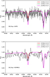 |
Fig. A.1. Example of spectral synthesis for C I line at 6587 in DQ Hya for both HERMES and UVES spectra. There is a remarkable agreement between the two estimates. We note that NLTE departures are negligible for this line, especially at the parameter range of our sample stars (Alexeeva & Mashonkina 2015). |
A.2. Abundance sensitivities for DQ Hya
We have calculated abundance sensitivities to stellar parameters for star DQ Hya. In Table A.3 we report the resulting variation in [X/Fe] for all the species to changes in Teff, log g, and Vmic.
Abundance sensitivities to change in stellar parameters for DQ Hya.
A.3. Orbital properties
In Table A.4 we present a summary of the orbital properties: eccentricity, maximum height above the disc, and membership likelihood (Eq. 1) to the thick disc (pthick), old thin disc (pthin, old; 7 < tage/Gyr < 10), intermediate-age thin disc (pthin, int; 3 < tage/Gyr < 5), and young thin disc (pthin, young; tage < 3 Gyr), as defined in Robin et al. (2003). Values in parentheses indicate the membership likelihoods computed without considering the metallicity. The reported values represent the mean over 105 orbit realisations by sampling the uncertainties on the astrometric and chemical properties of the stars. Uncertainties are not shown, as they are below the 10% level for the orbital parameters and 1% level for the membership. Different rows correspond to different Galactic potential models: McMillan (2017, M17), and Allen & Santillan (1991, AS91). For DQ Hya, two variations are reported, corresponding to orbital integrations using the current distance estimated either from the parallax or from the absolute magnitude. For ASAS J153830–6906.4, only the parallax-based distance estimate is considered.
Orbital properties.
A.4. Spectral Energy Distribution for DQ Hya
In Fig. A.3 we present the SED for star DQ Hya. Photometric data were obtained from GALEX (Martin et al. 2005), Gaia DR3 (Gaia Collaboration 2023), 2MASS (Skrutskie et al. 2006), and WISE (Wright et al. 2010). No indication of NUV excess was observed when comparing the measured SED with the Kurucz (Castelli & Kurucz 2003) atmospheric model corresponding to the star’s parameters.
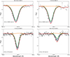 |
Fig. A.2. Example of spectral synthesis for Ba, Y, and Nd lines in DQ Hya. The orange lines represent nearly zero abundances for all the species in each panel. The blue lines denotate the best-fit abundances, while red and green lines are for ±0.2 dex, respectively. |
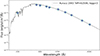 |
Fig. A.3. SED of DQ Hya, no excess in the GALEX NUV photometry is detected. |
All Tables
Stellar parameters and additional n-capture element abundances of DQ Hya from UVES spectra.
Line list (and corresponding atomic data) for parameter and abundance determinations in HERMES/GALAH spectra.
Additional line list for abundance determination of n-capture elements in UVES spectra for DQ Hya.
All Figures
|
Fig. 1. Comparison of the observed spectra from GALAH DR4 for our sample RRL DQ Hya (GALAH 170601002101298) and another RRL with very similar atmospheric parameters and metallicity by D’Orazi et al. (2024). |
| In the text | |
|
Fig. 2. Ratios of [Eu/Fe] vs. [La/Fe] for CEMP-r and CEMP-s stars by Masseron et al. (2010), CEMP-s stars by Roederer et al. (2014), Ba stars by Roriz et al. (2021), and the s-rich RRLs DQ Hya and TY Gruis. The dashed line is the 1:1 relationship. |
| In the text | |
|
Fig. 3. Ratios of [Ce/Y] as a function of metallicity [Fe/H]. |
| In the text | |
|
Fig. 8. Kiel diagram comparing the RR Lyrae stars analysed in this work (DQ Hya shown as a diamond, ASAS J153830−6906.4 as a square) with horizontal branch evolutionary tracks from the PARSEC V1.2S database (Chen et al. 2015, circles; masses and metallicities are indicated in the plot). The colour map represents the bolometric luminosity. For the observed stars, luminosities are derived using distances from parallaxes (see Sect. 4.1). The size of the circles along the tracks provides a qualitative indication of the time spent in each region of the diagram, with the largest symbols corresponding to approximately ten times longer evolutionary timescales than the smallest ones. The grey lines indicate the instability strip from Marconi et al. (2015), assuming a metallicity of Z = 0.002 and stellar masses of 0.56 M⊙ (dotted line) and 0.62 M⊙ (dashed line). The comparison is purely qualitative and does not represent the result of a fit. |
| In the text | |
|
Fig. 4. Integrated orbits of DQ Hya (thick solid line: distance from parallax inversion; dashed line: distance estimated from the RR Lyrae magnitude–metallicity relation) and ASAS J153830–6906.4 (thin solid line: distance from parallax inversion), computed using the Milky Way potential models by McMillan (2017, M17, left panel) and Allen & Santillan (1991, AS91, right panel). |
| In the text | |
|
Fig. 5. Comparison of the orbital properties, eccentricity, and maximum distance from the Galactic plane, of DQ Hya and ASAS J153830−6906.4 with the sample of disc stars from Bensby et al. (2014, B14). The contours represent the 68%, 95%, and 99.7% confidence intervals from 105 orbit realisations; line styles and colours follow those used in Fig. 4. Circle and square markers indicate stars classified by B14 as likely thin disc and thick disc members, respectively, based on a thick-to-thin disc likelihood ratio of < 0.5 and > 2. Star-shaped markers represent stars in between the two components with intermediate likelihood ratios. Both our orbit integrations and those in B14 adopt the Galactic potential from Allen & Santillan (1991). |
| In the text | |
|
Fig. 6. Comparison of observations with stellar models by FRUITY (Cristallo et al. 2011) and Monash groups (Karakas et al. 2018, and references therein). Symbols are the same as in Fig. 3. Masses are in M⊙. |
| In the text | |
|
Fig. 7. RUWE values (vertical dash–dot black lines) of the two analysed RR Lyrae stars (left: ASAS J153830−6906.4, right: DQ Hya) compared to the cumulative distribution functions of the corresponding control samples. The solid blue line shows the CDF for the sky-position control sample, which includes stars in the same sky area with similar photometry. The dotted blue line shows the CDF for the same sample after removing stars classified as non-single in Gaia DR3. The dashed red line shows the CDF for the RR Lyrae control sample from Gaia DR3, selected to have similar photometry and light-curve properties to the targets (see text for details). The shaded regions indicate the central 68% (dark shading) and 95% (light shading) intervals of the distributions. |
| In the text | |
|
Fig. A.1. Example of spectral synthesis for C I line at 6587 in DQ Hya for both HERMES and UVES spectra. There is a remarkable agreement between the two estimates. We note that NLTE departures are negligible for this line, especially at the parameter range of our sample stars (Alexeeva & Mashonkina 2015). |
| In the text | |
|
Fig. A.2. Example of spectral synthesis for Ba, Y, and Nd lines in DQ Hya. The orange lines represent nearly zero abundances for all the species in each panel. The blue lines denotate the best-fit abundances, while red and green lines are for ±0.2 dex, respectively. |
| In the text | |
|
Fig. A.3. SED of DQ Hya, no excess in the GALEX NUV photometry is detected. |
| In the text | |
Current usage metrics show cumulative count of Article Views (full-text article views including HTML views, PDF and ePub downloads, according to the available data) and Abstracts Views on Vision4Press platform.
Data correspond to usage on the plateform after 2015. The current usage metrics is available 48-96 hours after online publication and is updated daily on week days.
Initial download of the metrics may take a while.