| Issue |
A&A
Volume 704, December 2025
|
|
|---|---|---|
| Article Number | A160 | |
| Number of page(s) | 9 | |
| Section | Planets, planetary systems, and small bodies | |
| DOI | https://doi.org/10.1051/0004-6361/202557620 | |
| Published online | 15 December 2025 | |
High charge-state solar wind ions interacting with comet 67P/Churyumov-Gerasimenko
Observations and comet activity estimates
1
Swedish Institute of Space Physics,
981 92
Kiruna,
Sweden
2
Université d’Angers,
49000
Angers,
France
3
Institute of Physics, University of Graz,
Universitätspl. 5,
8010
Graz,
Austria
4
Space Research & Planetary Sciences, Physics Institute, University of Bern,
Sidlerstrasse 5,
3012
Bern,
Switzerland
★ Corresponding author: This email address is being protected from spambots. You need JavaScript enabled to view it.
Received:
9
October
2025
Accepted:
30
October
2025
Abstract
Context. Solar wind interacts with the atmospheres of planets, moons, and comets. One of the important interaction processes is charge exchange. High charge-state heavy ions in solar wind are prone to charge exchange with typical atmospheric constituents due to their large cross-sections. These processes are important for remote observations of comets through X-ray emissions.
Aims. We survey the ESA/Rosetta data for in situ observations of multiply charged oxygen ions and estimate the neutral outgassing rate of comet 67P/Churyumov-Gerasimenko through the fluxes of heavy ions such as O6+ and O5+.
Methods. We used data from the Ion Composition Analyzer on board the Rosetta spacecraft to obtain oxygen ion fluxes. We found the expected signal to be weak and therefore applied careful data filtering. We then adapted a pre-existing model to calculate the outgassing rate of the comet.
Results. We find that multiply charged oxygen ions are mostly found post perihelion. The estimated outgassing rate is QOth = 1.87 ⋅ 1028 × Rh−5.00 [s−1], with Rh being the heliocentric distance.
Conclusions. Our outgassing estimates agree well with estimates from previous studies based on observations of helium ions. Our work extends these previous studies through the use of a completely independent dataset with coverage until the end of the Rosetta mission and by taking the varying neutral gas composition into account. The ratio of oxygen-to-helium fluxes we determined also matches previous measurements. Our comparison to ROSINA neutral gas measurements shows that heavy solar wind ions, such as oxygen, can be used to retrieve the neutral gas activity of the comet when direct neutral gas observations are not available.
Key words: plasmas / instrumentation: detectors / solar wind / comets: general / comets: individual: 67P/Churyumov-Gerasimenko
© The Authors 2025
 Open Access article, published by EDP Sciences, under the terms of the Creative Commons Attribution License (https://creativecommons.org/licenses/by/4.0), which permits unrestricted use, distribution, and reproduction in any medium, provided the original work is properly cited.
This article is published in open access under the Subscribe to Open model. This email address is being protected from spambots. You need JavaScript enabled to view it. to support open access publication.
1 Introduction
Solar wind is the dynamical extension of the Sun’s atmosphere into the surrounding space (Parker 1965). The elemental composition of solar wind is a function of both the photospheric source and the processes that ionise, heat, and transport the photospheric constituents in the solar corona (von Steiger & Geiss 1989). Solar wind mainly contains protons, a few percent of doubly charged helium ions, and traces of heavier elements. In particular, there is an enrichment of elements with a low first ionisation potential (FIP) in the corona and solar wind as compared to the photosphere. The precise composition and charge state of solar wind reflects the temperature of the inner corona, the so-called freeze-in temperature (Hefti et al. 2000). In situ studies of solar wind composition can therefore provide clues related to the initial transport and acceleration processes in the solar corona as well as any further modifications of the solar wind caused during the transport through the heliosphere.
The solar wind speed distribution is essentially bimodal, being either a fast solar wind of typically 750 km/s or a slower more variable solar wind with a speed of about 400 km/s. The FIP-related enrichment is most pronounced for the slow solar wind, with an enhancement of a factor of three to four of low FIP elements as compared to the photosphere (Feldman et al. 2005). As a consequence, helium ions (alpha particles) with a comparably large FIP of 24.6 eV are less abundant in the slow solar wind, though there is a variation with the solar cycle as well (Aellig et al. 2001).
Multiply charged oxygen ions form a minor part of solar wind, with an abundance of about three orders of magnitude lower than that of protons. Oxygen fluxes in solar wind as observed by the Ulysses spacecraft were reported by von Steiger et al. (2010). They found that the proton-to-oxygen ratio in fast streams is  , compared to
  for the slow solar wind. The intervals given contain 67% of the observations (1 σ). Extreme fluxes of oxygen ions are thus more likely for a slow solar wind. von Steiger et al. (2010) used O7+-to-O6+ and C6+- to-C5+ charge-state ratios to determine the solar wind type rather than the usual discrimination based on bulk velocity (‘fast’ and ‘slow’). This method is superior but not always available. Carpenter et al. (2024); Zhao et al. (2024) studied the charge-state distribution of oxygen ions as a function of the solar wind speed. They found that O6+ is by far the dominating oxygen charge state for fast winds, at 95% relative abundance and dropping to 72% for slow solar wind. The second most abundant charge state is O7+, at 5 and 20%, respectively.
When solar wind propagates through space, it interacts with the bodies it encounters. These bodies range from planets, their atmospheres, and magnetospheres to smaller bodies such as natural satellites, asteroids, and comets. These obstacles affect the solar wind (Barabash 2012). In this study, we are concerned with the interaction of solar wind with comets.
Comets are composed mainly of ices and dust. When a comet approaches the Sun, its surface heats up, and the ices begin to sublimate, initially mostly liberating CO2 and CO (A’Hearn et al. 2012). This sublimation and liberation of gas lead to the creation of the cometary atmosphere. Close to perihelion, the comet reaches the peak of its activity, where sublimation of water ice takes the lead over CO2 and CO, and H2O becomes the prominent species within the neutral coma (Can et al. 2023).
When solar wind encounters a cometary atmosphere, a number of chemical reactions take place. These reactions change the chemical composition and affect the dynamics of the solar wind near the coma. One important process is the charge exchange (Gombosi 1987; Dennerl 2010). Charge exchange is a chemical process in which two species interact with each other and one or multiple electrons are exchanged. All ions present in the solar wind thus react with the neutral atmosphere surrounding the comet and produce ions with lower charge states through solar wind charge exchange (Bodewits & Hoekstra 2007; Simon Wedlund et al. 2016).
High charge-state oxygen ions in solar wind can give rise to X-ray emissions through charge-exchange reactions, as first seen for comets (Cravens 1997; Haberli et al. 1997) and later also for Mars (Dennerl et al. 2006). Thus X-ray emissions can be used to study high charge-state ion abundance in the solar wind (Deskins & Bodewits 2023).
The outgassing rate of a comet is defined by the number of molecules per second expelled from the nucleus due to the sublimation of the ices composing it. The ices are composed of different species with different sublimation temperatures, and the outgassing profile of the comet varies with the distance to the Sun (Fink et al. 2016). Multiple remote ways of calculating this value have been explored, from the use of X-rays and extreme UV (McCauley et al. 2013; Snodgrass et al. 2017) and far infrared (de Val-Borro et al. 2014) spectroscopy to obtain column densities and then the outgassing rates of H2O and/or NH3 to the use of radio telescopes (Biver et al. 1997; Bockeleee-Morvan et al. 2001). At comet 67P, the Rosetta mission collected in situ measurements that enable other more direct ways of deriving the outgassing rate by measuring the gas itself. Gulkis et al. (2015) and Biver et al. (2019) have determined the outgassing rate of H2O and other neutral species using the Microwave Instrument on Rosetta Orbiter (Gulkis et al. 2006). Hansen et al. (2016), Gasc et al. (2017), and Combi et al. (2020) have all estimated the outgassing rate of various neutral species using the Rosetta Orbiter Spectrometer for Ion and Neutral Analysis (Balsiger et al. 2007, ROSINA;) instrument(s). Finally, the variation in abundance of different low charge-state ions in solar wind can be used as a tool to probe the cometary atmosphere. Simon Wedlund et al. (2016, 2019c,a,b) used the data from the Ion Composition Analyzer (Nilsson et al. 2006, ICA) to get an estimate of the atmospheric column density upstream of the observation point using the He+ to He2+ ratio from which an outgassing rate could then be obtained.
This study focuses on O6+ and O5+ ions around comet 67P observed by the ion mass spectrometer ICA. The second most important oxygen ion, O7+, is unfortunately nearly impossible to distinguish from other species with the energy and mass resolution of ICA. We surveyed the entire mission for observations of O6+ and O5+. Our aim is to estimate the outgassing rate, Q0, of the comet using oxygen ion fluxes and compare our estimates with an already established model of the outgassing of comet 67P (Simon Wedlund et al. 2016, 2019b).
2 Description of instruments
For this study, we used data from the ICA, the magnetometer, and ROSINA of the Rosetta spacecraft. All data are publicly available in The European Space Agency’s Planetary Science Archive (PSA).
2.1 Ion Composition Analyzer
The ICA is a mass spectrometer that is part of the Rosetta Plasma Consortium (RPC) package (Carr et al. 2007). It is designed to measure the velocity distribution of ions (Nilsson et al. 2006). It features a field of view spanning 360° in azimuth and 90° in elevation divided into 16 angular bins, resulting in an angular resolution of 22.5° in azimuth and approximately 5.6° in elevation. It features a wide energy range from a few electronvolt per charge to 40 keV/q with a resolution of ∆E/E = 0.07, where q is the elementary charge. The ICA provides mass per charge resolved ion data, distinguishing between H+, He2+, and He+ and heavier ions such as H2O+ and  . The full observation space, noted as Θ, covered by the instrument can thus be described as a four-dimensional matrix of the following shape: azimuth × energy × mass × elevation. Azimuth and mass are measured simultaneously, while different energy and elevation settings are sequentially electrostatically scanned. A full scan of Θ is performed in 192s, the temporal resolution of the instrument.
For this study, we used the PSA Rosetta Plasma Consortium (RPC)-ICA L2 dataset consisting of the lowest-level processed data that were only processed to be human readable. By using these data, we avoided any further processing that would affect the supposedly weak signals of O6+ and O5+.
2.2 Complementary instruments: Magnetometer and ROSINA
The magnetometer instrument measures the magnetic field vectors in a range of ±16384 nT with a resolution of 31 pT Glassmeier et al. (2007). ROSINA is an instrument suite designed to measure abundances of ions and neutral atoms and molecules locally at the location of Rosetta (Balsiger et al. 2007). We used data derived from a combination of the ROSINA Double Focusing Mass Spectrometer and Comet Pressure Sensor to obtain abundances of the two major neutral gas species H2O and CO2. Details on the derivation of the total and relative abundances of neutral gas species are available in Rubin et al. (2019).
3 Observations of a weak signal
We used data from the entire Rosetta mission. Rosetta followed the comet when approaching the Sun (inbound phase), through perihelion, and when the comet moved away from the Sun (outbound phase; Fig.1c). The cometocentric distance changed depending on the activity of the comet, which is linked to the heliocentric distance (Glassmeier et al. 2007).
The ICA dataset is composed of both the signals that we are looking for and background noise. The oxygen ion signal is likely weak and intermittent (Nilsson et al. 2015) and can be lost in the background noise or in the tails of the strong signals surrounding them. To extract this signal, we needed to reduce the background noise and select the right time instances. Our pipeline for the preparation of the data is split into six steps, which we detail in the following.
Time instances selection: during the mission, the instrument used different modes, and each had a different energy, mass, and angular and/or time resolution (Nilsson et al. 2006, 2017). ICA measures fluxes versus angles and energy, with the latter based on the mass-to-charge ratio so that the O6+ (m/q=16/6) and O5+ (m/q=16/5) signals are expected to be at a typical m/q between He2+ (m/q = 2) and He+ (m/q = 4). Since our signal is small in parameter space and constrained between two large signals (He+ and He2+) in energy space, we only included data with the highest energy, mass, and angular resolution possible. We also excluded data taken in the solar wind ion cavity, a time period spanning 6 months around perihelion and where the solar wind ions were not observed by ICA (Behar et al. 2017). All remaining time instances can be found in Fig. 1a.
Angular selection: the instrument field of view is partially obstructed by the spacecraft, namely, azimuth bins 0, 1, and 9–15 for elevation bins 0–10 (Bergman et al. 2021). Moreover, Canu-Blot et al. (2024) found that the azimuth bins 2 and 3 have a significantly higher level of crosstalk than the other bins. We thus only kept azimuth bins 4–8 for data collection. We only selected the data from angular bins whose boresight were directed towards the sun within an acceptance angle of 45° centred about the Sun direction. We used the Sun direction as a proxy for the solar wind direction. Because of their lower charge-to-mass ratios, solar wind oxygen ions are less deflected than helium ions in the mass-loaded plasma environment of the comet (Behar et al. 2016, 2017), and thus their direction is not much different from the Sun direction. Moreover, modification of the acceptance angle to a higher value (60°) did not change the number of observations of multiply charged oxygen ions, which further justifies this approximation. To estimate the background, we created another set of data from angular bins with boresight directed away from the Sun to minimise contamination from solar wind oxygen ions. We used a wide anti-sunward acceptance angle of 90°.
Mass-energy selection: we used the calibrated energy-dependent mass responses (Fig. 2), and we estimated the approximate energy and mass bins where O5+ and O6+ ions are expected to be visible (Nilsson et al. 2006). The energy at which we expected to see O5+ and O6+ was estimated from the assumption that all solar wind ions travel at the same speed. In reality, it has been shown that heavy ions flow faster than lighter ones by up to the Alfven speed, though this represents only a few tens of kilometres per second and is negligible given the energy resolution of ICA (Berger et al. 2011). The solar wind speed was estimated from the strong alpha particle signal. The alpha particle signal has the advantage over the H+ signal in that if there is any slowing down of the solar wind due to the interaction with the comet environment, then the alpha particle speed will be more similar to the oxygen ion speed than the H+ speed (Nilsson et al. 2022) These energy-dependent mass lines were obtained from the instrument calibration of ICA. These estimations are presented in Fig. 2.
Removal of the strong signals: our two oxygen ion signals are located between the He2+ and He+ signals in energy-per-charge space, with few energy bins between each signal. To avoid pollution from these signals, we removed them by fitting a kappa distribution to the He+ and He2+ signals. We added these fits to the background dataset for further statistical subtraction. A kappa distribution with 4 degrees of freedom was selected empirically as giving the best fit to the data compared to a Gaussian or a Maxwellian distribution.
Background noise reduction: The last step was the statistical subtraction of the background using the method proposed by Feldman & Cousins (1998) and described in detail by Canu-Blot et al. (2024). The average number of signal counts was estimated from the centre of the 68% (1σ) confidence interval, with error bars describing the 90% confidence interval.
The steps above were applied to 15 minute time intervals, which may include one to five scans, depending on the filter criteria. From this survey we found 90 observations of O6+ and O5+. Figure 1b shows all observations as green lines. Most of these observations (83) are in the outbound phase of the comet orbit. To keep a homogeneous dataset, we only studied these 83 observations since the comet did behave differently when inbound and outbound, i.e. in its outgassing activity of the different neutral gas species (Combi et al. 2020; Läuter et al. 2020).
Figure 3 shows an example of the differential flux spectrum resulting from all the aforementioned steps, with the conversion from counts to flux. The oxygen ion signals as well as the kappa distribution fitted to the He2+ and He+ signals can be clearly seen.
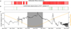 |
Fig. 1 Overview of observations of O6+ and O5+ at comet 67P during the Rosetta mission. (a) Time instances analysed in the study, represented by red lines. (b) Instances where O6+ and O5+ are observed, represented by green lines. (c) Cometocentric and heliocentric distance for the entire Rosetta mission. The solar wind cavity is symbolised by the grey area. The large cometocentric distance at the end of March 2016 is due to the nightside excursion (Behar et al. 2018). |
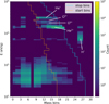 |
Fig. 2 Energy per charge (y-axis) per mass bin matrix. The data shown here come from 21 March 2016 between 17:45 and 18:00 UTC. The cyan and orange lines are the energy-dependent mass responses for molecules of mass per charge 16/6 and 16/5 respectively. Only the data between the two lines was kept for data integration. |
4 Helium-to-oxygen ratio
We compared the observed oxygen fluxes to the simultaneously observed helium fluxes. These fluxes are the total ion fluxes, meaning that they are the sum of the fluxes of all observed charge states of oxygen and helium. Figure 4 shows the ratio of the total helium fluxes to the total oxygen fluxes versus the solar wind speed. The colour bar shows the heliocentric distance of each point. We did not observe a correlation between the heliocentric distance and the ratio of helium to oxygen ions. A power-law fit (axb, with a and b as the fit parameters) was applied to the data, showing an average ratio of around one hundred. Collier et al. (1996) used measurements from the WIND spacecraft to compute the ratios between different solar wind ions (shown as orange squares in Fig. 4). They found a ratio between helium and oxygen comparable to ours.
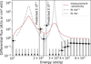 |
Fig. 3 Ion differential fluxes with the background removed versus energy per charge (black dots). The data shown here come from 21 March 2016 between 17:45 and 18:00 UTC, shown in Fig. 2. The red line represents the measurement sensitivity, indicating the minimum flux for an observation to be considered statistically different from the background. The dash grey lines represents the fitted function that we subtracted from the matrix. The fits are only shown for the relevant energies. The vertical dashed black lines are the estimated energies of O6+ and O5+, respectively. The vertical lines match the energy of the observed data points well. These estimated energies were calculated assuming a uniform solar wind speed between species. The vertical error bars are the 90% confidence interval computed during the background noise reduction, with the horizontal error bar representing the energy resolution. |
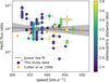 |
Fig. 4 Ratio of the total helium fluxes to total oxygen fluxes versus the solar wind speed as well as a the power-law fit (black dashed line) and its ±σ confidence interval (in grey). The colour bar represents the heliocentric distance of each data point. The data from Collier et al. (1996) are shown in orange. |
5 Neutral outgassing rates
The vast majority of the oxygen in solar wind is O6+, accounting for 72 to 92% of the total population, but there are traces of O5+, O7+, and O8+ (Carpenter et al. 2024). The O5+ makes up around 2% of the total population. From Fig. 3, where O6+ accounts for about 47% and O5+ for about 53% of the visible oxygen population, we inferred the presence of a process converting O6+ and/or other charge states into O5+. This process is a charge exchange that occurs between solar wind ions and neutral atoms and molecules in the coma. Such interactions can be used to estimate the outgassing rate, that is, the total number of neutral atoms expelled by the comet. Simon Wedlund et al. (2016) and Simon Wedlund et al. (2019b) used helium ion fluxes to estimate the outgassing rate of the comet, and we adapted their method to estimate the outgassing rate using oxygen ion fluxes instead.
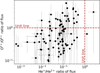 |
Fig. 5 Correlation between the ratio of oxygen ion fluxes and helium ion fluxes. There is a weak log correlation of 0.4 (p-value of 1e−4). |
5.1 Analytical model
5.1.1 Charge-exchange process
The charge-exchange process is described by the following reaction:
 (1)
with A as a solar wind ion, B as a cometary neutral species, m as the starting charge of the solar wind ion, and n as the number of charge(s) exchanged between particles.
(1)
with A as a solar wind ion, B as a cometary neutral species, m as the starting charge of the solar wind ion, and n as the number of charge(s) exchanged between particles.
A way to measure the efficiency of this process is by calculating the ratio of particle fluxes at a distance, r, from the comet, RA(r), given the particle fluxes  and
and  , both in #/(sr s cm2 eV) (Nilsson et al. 2015):
 (2)
(2)
We computed this ratio for all observations of O5+ and O6+. We did the same for helium fluxes. Figure 5 shows the ratio of the oxygen ion fluxes compared to the ratio of the helium ion fluxes for each 15 minute observation. The correlation that we observed is expected since the populations of O5+ and He+ are generated by the same process. Moreover, we noted that the ratio for the oxygen ions is often tenfold that of the helium ions, hinting at a process that is more likely to occur for oxygen. Table 1 supports this observation, where cross-sections for the charge-exchange process for O6+ and He2+ with H2O and CO2 are given at a typical impact speed of 400 km/s. The charge-exchange cross-sections for the oxygen ions are approximately 3.5–11 times higher than those of the helium ions.
Charge-exchange cross-sections.
5.1.2 Charge-exchange cross-sections
We used our observations to estimate the outgassing of comet 67P. The two most prominent species in the coma are H2O and CO2, with H2O dominating during most of the mission and CO2 taking over in the later stage of the mission (Combi et al. 2020; Rubin et al. 2023; Läuter et al. 2020). We considered only the reaction between the solar wind ions and these two neutral species, with the total neutral density being the sum of the two.
The oxygen population is composed of ions with different charge states, and multiple reactions come into play for the generation of O5+. However, as stated previously, the populations of some of the other charge states of oxygen (O5+ and O8+) are very small relative to O6+, and thus we could ignore them. Because of small abundances compared to O6+, we assumed that the initial O5+ and O8+ populations are negligible in the undisturbed solar wind and that the O5+ ions present in the coma only come from charge exchange of O6+ ions. The O7+ population accounts for around an eighth of the total oxygen population, which gives it a relatively important role in the charge-exchange process. However, this ion has a mass-to-charge ratio of m/q = 16/7 2.29, placing its signal within the tail of the He2+ peak (m/q =≃2). As a result, it cannot be distinguished from the He2+ signal, and its flux cannot be reliably determined. We therefore assumed the entire O7+ population would be converted to O6+. This was motivated by the fact that the charge-exchange process becomes more effective with higher charge states (Friedman & DuCharme 2017). We thus considered the full population of oxygen ions after interaction to be composed of only the q = 5 and q = 6 charge states.
To summarise, we assumed that (i) H2O and CO2 are the only neutral species present in the cometary atmosphere and are at rest with respect to the comet. (ii) The population of O5+ and O8+ are non-existent before the interaction. (iii) 100% of the O7+ population is converted to O6+ or O5+. (iv) The entire population of oxygen, after interaction with the coma, is only composed of O6+ and O5+.
5.1.3 Outgassing rates estimates Q0
The total charge exchange experienced by the solar wind ions is a function of the neutral gas column density the solar wind has passed through and the charge-exchange cross-section. The latter is known, providing the possibility to estimate the former. From Simon Wedlund et al. (2016), we obtained the column density, Cdens[m−2], as
 (3)
with
(3)
with ![Mathematical equation: ${\sigma _{{A^{m + }}}}\left[ {{{\rm{m}}^2}} \right]$](/articles/aa/full_html/2025/12/aa57620-25/aa57620-25-eq10.png) as the cross-section of the ion Am+ assumed constant across the relevant energies and with their values at 830 eV/amu. We then calculated the outgassing rate Q0[s−1], assuming a spherically symmetric outgassing profile as
as the cross-section of the ion Am+ assumed constant across the relevant energies and with their values at 830 eV/amu. We then calculated the outgassing rate Q0[s−1], assuming a spherically symmetric outgassing profile as
 (4)
with v0 [m s−1] as the speed of the neutral particles; r(x, y, z) [m] as the position of the spacecraft in the comet-centred solar orbital system coordinates, with the x-axis pointed towards the Sun; rc[m] as the radius of an approximated spherical comet; and
(4)
with v0 [m s−1] as the speed of the neutral particles; r(x, y, z) [m] as the position of the spacecraft in the comet-centred solar orbital system coordinates, with the x-axis pointed towards the Sun; rc[m] as the radius of an approximated spherical comet; and ![Mathematical equation: $k_p^T\left[ {{{\rm{s}}^{ - 1}}} \right]$](/articles/aa/full_html/2025/12/aa57620-25/aa57620-25-eq12.png) as the photo-destruction rates of the neutral species. The photo-destruction products of H2O were not taken into account for the charge-exchange process because these products will photo-ionise quickly after dissociation. We focused on the total column density up to the position of Rosetta. In the photodissociation process, there is no loss of matter, and because H and OH should have similar – but smaller – charge-exchange cross-sections than H2O, the approximation made on the total retrieved outgassing rate at the position of Rosetta is negligible. For the retrieval of the H2O densities, we obtained an excellent agreement between H2O from this model with He+/He2+ ratios and the in situ observations with ROSINA, which implies that the dissociation products play only a minor role at best in the charge exchange.
as the photo-destruction rates of the neutral species. The photo-destruction products of H2O were not taken into account for the charge-exchange process because these products will photo-ionise quickly after dissociation. We focused on the total column density up to the position of Rosetta. In the photodissociation process, there is no loss of matter, and because H and OH should have similar – but smaller – charge-exchange cross-sections than H2O, the approximation made on the total retrieved outgassing rate at the position of Rosetta is negligible. For the retrieval of the H2O densities, we obtained an excellent agreement between H2O from this model with He+/He2+ ratios and the in situ observations with ROSINA, which implies that the dissociation products play only a minor role at best in the charge exchange.
To account for both neutral molecules in the coma, we computed a new cross-section, σtot[m2], as well as a new photodestruction rate defined by the following weighted averages:
 (5)
(5)
 (6)
with
(6)
with  and
and  as the density of both neutral species measured locally at Rosetta. We note that
  is scaled to the heliocentric distance, Rh, of comet 67P. For these formulae, a ratio of H2O to CO2 must be assumed. We used a time dependent ratio provided by ROSINA to be as close as possible to reality. In other cases, an estimation of the ratio using previous measurements or from models could be used. From Eqs. (5) and (6), it might appear that the cross-sections depend on the absolute neutral densities. This is not the case. Only the relative densities matter, as we made the assumption that the total neutral density is
  , with
 (7)
(7)
The photo-destruction rates at 1 AU are given in Table 2. The rate for any heliocentric distance, Rh, was obtained through the inverse-square law. The column density was then given by Eq. (3) when σA+ was replaced by the previously calculated value of σtot.
The last unknown to consider was the speed v0 [m s−1] of the neutral particles. In this study, we used an empirical model from Hansen et al. (2016) that gives the speed of the neutral particles, all of which were assumed to be travelling at the same speed, during the outbound period of the mission:
 (8)
(8)
All the constants used to compute the outgassing rates of the comet have been collected in Table 2.
Constants used in the Q0 calculations.
5.2 Dependence on the heliocentric distance
Figure 6a shows the outgassing estimates obtained from Eq. (4) using all observations of oxygen ions in the outbound phase. We also show the results of the same method applied to helium ions at the same points in time. We fitted an exponential fit  to the datasets, yielding
 (9)
and
(9)
and
 (10)
with Rh as the heliocentric distance. We note that our data and fits are in good agreement with the fits obtained by Simon Wedlund et al. (2016, 2019b). The oxygen and helium fits agree well, although there are differences (see Fig. 6a), but they are most likely due to isolated events. For example, the helium signal could have moved out of the field of view of the instrument, leading to lower observed fluxes. Figure 6b compares the outgassing rate estimates obtained from both the helium and oxygen ion observations with the outgassing rate estimates obtained using ROSINA data. The data points for ROSINA estimates are aggregates of roughly 15 minutes of data, consistent with the data points from ICA. The same exponential fit was applied to ROSINA data, yielding
(10)
with Rh as the heliocentric distance. We note that our data and fits are in good agreement with the fits obtained by Simon Wedlund et al. (2016, 2019b). The oxygen and helium fits agree well, although there are differences (see Fig. 6a), but they are most likely due to isolated events. For example, the helium signal could have moved out of the field of view of the instrument, leading to lower observed fluxes. Figure 6b compares the outgassing rate estimates obtained from both the helium and oxygen ion observations with the outgassing rate estimates obtained using ROSINA data. The data points for ROSINA estimates are aggregates of roughly 15 minutes of data, consistent with the data points from ICA. The same exponential fit was applied to ROSINA data, yielding
 (11)
(11)
Our estimates also agree with the simplified outgassing model derived from the ROSINA data.
6 Discussion
As is clear form Fig.1b, we observed more multiply charged oxygen ions during the outbound phase of the mission. One reason for this is that the total amount of time instances that we consider is greater post perihelion, although this may be an observation bias (Fig.1a). This disparity is visible through the ratio of confirmed observations over time instances, with about 0.2% before perihelion versus about 2% after perihelion. If we look at the total availability of oxygen in the ICA data compared to verified He2+ observations, we obtain a ratio of about 0.5% on the full Rosetta mission. These two ratios show that we do have a bias towards post-perihelion observations, where oxygen ions are more often observed. This bias may result from observational bias in the near-cometary environment; however, no clear correlation has been identified.
The oxygen observations may be correlated with specific solar wind conditions. To check this, we compared the distributions of the solar wind parameters for the entire mission with the distributions for the time instances where solar wind oxygen ions are observed. All data used in (Fig. 7) come from the instruments on board Rosetta. Figure 7a shows no real difference between the mean bulk speeds. However, no oxygen ions were observed for solar wind speeds greater than 500 km/s, which is consistent with von Steiger et al. (2010). The cone angle (Fig.7b), that is, the angle between the interplanetary magnetic field and the Sun direction, is also statistically similar. Figures 7c and d show that the helium density and the amplitude of the magnetic field are slightly higher when we observe oxygen ions. The bias towards greater helium densities is possibly because low helium fluxes would mean low oxygen fluxes, and these would fall below the detection threshold. Regarding the magnetic field amplitude, we observed a lack of very low values, whereas high values are more common. This could be related to the source at the Sun, where ions are kept in the ionisation zone for a longer time, thus allowing for more low FIP ions. It has been shown by Goetz et al. (2017) that the magnetic field does not vary much with the cometocentric distance. However, a strong magnetic field may correlate with a higher outgassing rate (higher production of O5+) due to the resulting stronger magnetic pile-up (Behar et al. 2016).
Our analysis yields a power-law fit dependent on the heliocentric distance,  , closely matching the fit found by Simon Wedlund et al. (2019b) for helium ions, where Rh is the heliocentric distance in AU. These similar results suggest that charge-exchange processes in the solar wind–coma interaction region are governed by similar physics, regardless of the species used to calculate the outgassing rate. The results also imply that multiple electron-capture events are negligible under the conditions observed around comet 67P. Specifically for oxygen, it indicates that the approximation of a full conversion of O7+ to O6+ is reasonable. From an observation point of view, this is very fortunate, as the O7+ population is very hard to detect with ICA.
We note that our filtering criteria means we only consider azimuthal bins 4–8. This choice removes some of the observations made in the direction towards the Sun. The Sun direction varies and is sometimes located in azimuthal bins 9 and 10. In such cases, we only took part of the signal within 45° from the Sun into account. Our choice to remove bins 9 and 10 minimises the noise but may have removed some detections of solar wind oxygen ions. However, as the helium-to-oxygen ratio agrees well with (Collier et al. 1996) and our outgassing rates agree with previous estimates (Simon Wedlund et al. 2019b), we conclude the effect is minor.
We argue that oxygen ions can be effectively used to estimate the outgassing rate of comet 67P despite being a weak signal. Moreover, the ability to compute neutral gas properties from heavy ion measurements makes it possible to analyse solar wind interaction processes in environments where neutral gas measurements are hard to obtain and light ions are rare or affected by instrumental limitations. For example, spacecraft outgassing and background (Schläppi et al. 2010) can lead to difficulties deriving abundances of gases of cometary origin, especially for large cometocentric distances and/or low production rates.
By using high charge-state solar wind ions, we provide a new independent estimate of outgassing compared to the modelled activity based on local neutral density measurements (Hansen et al. 2016). Our results are also based on the signal of another ion, oxygen, and associated charge-exchange cross-section estimates, as compared to previously published results based on helium (Simon Wedlund et al. 2016, 2019b). In contrast to such previous estimates of the outgassing, we take the changing neutral composition of the cometary atmosphere into account. The difference is small in our case, but visible. Our data based both on charge exchange and local neutral density extends the results of Hansen et al. (2016) to the end of the Rosetta mission (see also Gasc et al. 2017). The outgassing rate falls off slowly with heliocentric distance beyond a distance of about 3 AU Combi et al. (2020); Läuter et al. (2020). This coincides with where CO2 becomes more prevalent. This slow decay in the outgassing rate is also observed in the ROSINA measurements from the approach phase (early mission), as seen in Hansen et al. (2016, Fig. 9).
The model applied in this study involves simplifications of some physical aspects, which may influence the results. It is thus possible to further improve the model. An obvious addition is to add other charge states of oxygen, such as O7+ or O4+. One could also take into account other ways in which oxygen ions can interact with neutral species by charge exchange, for example, adding two-electron capture. Considering more neutral species for the charge-exchange process could further refine the accuracy of the model. In fact, at heliocentric distances beyond 3 AU, species such as CO or even H2S become a non-negligible part of the total neutral gas density (Gasc et al. 2017). However, cross-sections for more complex molecules are not always available.
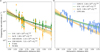 |
Fig. 6 Outgassing rate estimates from different sources as a function of the heliocentric distance. Panel a: outgassing rate estimates as a function of the heliocentric distance obtained from oxygen ions and helium ions in green and orange, respectively. The fits from Simon Wedlund et al. (2016) and Simon Wedlund et al. (2019b) are shown in grey and black dashed lines, respectively. The green and orange areas represents the 90% confidence interval of the fits. Panel b: outgassing rate estimates obtained from both helium and oxygen ion particle fluxes and from ROSINA data in orange, green, and blue, respectively, plotted against the heliocentric distance, Rh. The green and blue areas represents the 90% confidence interval of the fit. |
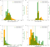 |
Fig. 7 Speed distribution (a), cone angle of the magnetic field (b), alpha particle density (c), and magnetic field amplitude (d) of the solar wind over the full mission (orange) and for our observations (green) with their respective mean value in dashed lines. All histograms have been normalised. |
7 Conclusion
We have presented, for the first time, detections of O6+ and O5+ from the RPC/ICA ion spectrometer data at comet 67P during the ESA/Rosetta mission. Most of the observations occurred post-perihelion. The helium-to-oxygen ion ratio was about 100, in agreement with Collier et al. (1996). During these observations, the magnitude of the magnetic field was noticeably higher than during the mission as a whole, with greater values being more prevalent during high charge-state solar wind ion observations. This is also visible through the mean values, which are 15.877 nT for the entire mission compared to 25.605 nT for our observations.
We used the ratio of O5+ to O6+ to estimate the local neutral outgassing rate  from comet 67P. We find that the outgassing rate as a function of the heliocentric distance can be expressed as
  . Our result is in excellent agreement with Simon Wedlund et al. (2016, 2019b). We also find that QO decays rather slowly at heliocentric distances beyond 3 AU based on both our method and ROSINA neutral density estimates. Assuming a multi-species neutral atmosphere in our model improved the agreement between our outgassing rate and ROSINA outgassing rate estimates.
Data availability
A table with all oxygen ions observations used in this study is available at the CDS via https://cdsarc.cds.unistra.fr/viz-bin/cat/J/A+A/704/A160.
Acknowledgements
The work of C.S.W. was funded by the Austrian Science Fund (FWF) 10.55776/P35954. The operation of the ICA instrument was funded by grant 108/12 from the Swedish National Space Board.
Reference
- Aellig, M. R., Lazarus, A. J., & Steinberg, J. T. 2001, GRL, 28, 2767 [NASA ADS] [CrossRef] [Google Scholar]
- A’Hearn, M. F., Feaga, L. M., Keller, H. U., et al. 2012, ApJ, 758, 29 [CrossRef] [Google Scholar]
- Balsiger, H., Altwegg, K., Bochsler, P., et al. 2007, SSRv, 128, 745 [Google Scholar]
- Barabash, S. 2012, EPS, 64, 57 [Google Scholar]
- Behar, E., Lindkvist, J., Nilsson, H., et al. 2016, A&A, 596, A42 [NASA ADS] [CrossRef] [EDP Sciences] [Google Scholar]
- Behar, E., Nilsson, H., Alho, M., Goetz, C., & Tsurutani, B. 2017, MNRAS, 469, S396 [Google Scholar]
- Behar, E., Nilsson, H., Henri, P., et al. 2018, A&A, 616, A21 [NASA ADS] [CrossRef] [EDP Sciences] [Google Scholar]
- Berger, L., Wimmer-Schweingruber, R. F., & Gloeckler, G. 2011, Phys. Rev. Lett., 106, 151103 [NASA ADS] [CrossRef] [Google Scholar]
- Bergman, S., Stenberg Wieser, G., Wieser, M., et al. 2021, MNRAS, 507, 4900 [NASA ADS] [CrossRef] [Google Scholar]
- Biver, N., Bockelée-Morvan, D., Colom, P., et al. 1997, EM & P, 78, 5 [Google Scholar]
- Biver, N., Bockelée-Morvan, D., Hofstadter, M., et al. 2019, A&A, 630, A19 [NASA ADS] [CrossRef] [EDP Sciences] [Google Scholar]
- Bockeleee-Morvan, D., Biver, N., Moreno, R., et al. 2001, Science, 292, 1339 [Google Scholar]
- Bodewits, D., & Hoekstra, R. 2007, Phys. Rev. A, 76, 032703 [Google Scholar]
- Can, L., Yu-hui, Z., & Jiang-hui, J. 2023, Chin. Astron. Astrophys., 47, 637 [Google Scholar]
- Canu-Blot, R., Wieser, M., & Wieser, G. S. 2024, A&A, 683, A245 [NASA ADS] [CrossRef] [EDP Sciences] [Google Scholar]
- Carpenter, D. T., Lepri, S. T., Zhao, L., et al. 2024, Front. Astron. Space Sci., 11 [Google Scholar]
- Carr, C., Cupido, E., Lee, C. G. Y., et al. 2007, SSRv, 128, 629 [Google Scholar]
- Collier, M. R., Hamilton, D. C., Gloeckler, G., Bochsler, P., & Sheldon, R. B. 1996, GRL, 23, 1191 [Google Scholar]
- Combi, M., Shou, Y., Fougere, N., et al. 2020, Icarus, 335, 113421 [NASA ADS] [CrossRef] [Google Scholar]
- Cravens, T. E. 1997, GRL, 24, 105 [Google Scholar]
- de Val-Borro, M., Bockelee-Morvan, D., Jehin, E., et al. 2014, A&A, 564, A124 [NASA ADS] [CrossRef] [EDP Sciences] [Google Scholar]
- Dennerl, K. 2010, SSRv, 157, 57 [Google Scholar]
- Dennerl, K., Lisse, C., Bhardwaj, A., et al. 2006, A&A, 451, 709 [NASA ADS] [CrossRef] [EDP Sciences] [Google Scholar]
- Deskins, T., & Bodewits, D. 2023, AAS Meeting Abstr., 241, 104.18 [Google Scholar]
- Feldman, G. J., & Cousins, R. D. 1998, Phys. Rev. D, 57, 3873 [NASA ADS] [CrossRef] [Google Scholar]
- Feldman, U., Landi, E., & Schwadron, N. A. 2005, JGR: Space Phys., 110, A7 [Google Scholar]
- Fink, U., Doose, L., Rinaldi, G., et al. 2016, Icarus, 277, 78 [Google Scholar]
- Friedman, B., & DuCharme, G. 2017, J. Phys. B, 50, 115202 [Google Scholar]
- Gasc, S., Altwegg, K., Balsiger, H., et al. 2017, MNRAS, 469, S108 [Google Scholar]
- Glassmeier, K.-H., Richter, I., Diedrich, A., et al. 2007, SSRv, 128, 649 [Google Scholar]
- Goetz, C., Volwerk, M., Richter, I., & Glassmeier, K.-H. 2017, MNRAS, 469, S268 [NASA ADS] [CrossRef] [Google Scholar]
- Gombosi, T. I. 1987, GRL, 14, 1174 [Google Scholar]
- Greenwood, J. B., Mawhorter, R. J., Cadez, I., et al. 2004, Phys. Scr., 110, 358 [Google Scholar]
- Gulkis, S., Frerking, M., Crovisier, J., et al. 2006, SSRv, 128, 561 [Google Scholar]
- Gulkis, S., Allen, M., von Allmen, P., et al. 2015, Science, 347, aaa0709 [Google Scholar]
- Haberli, R. M., Gombosi, T. I., De Zeeuw, D. L., Combi, M. R., & Powell, K. G. 1997, Science, 276, 939 [Google Scholar]
- Han, J., Wei, L., Wang, B., et al. 2021, ApJS, 253, 6 [Google Scholar]
- Hansen, K. C., Altwegg, K., Berthelier, J.-J., et al. 2016, MNRAS, 462, S491 [Google Scholar]
- Hefti, S., Grunwaldt, H., Bochsler, P., & Aellig, M. R. 2000, JGR: Space Phys., 105, 10527 [Google Scholar]
- Huebner, W., & Mukherjee, J. 2015, PSS, 106, 11 [Google Scholar]
- Kusakabe, T., Miyamoto, Y., Kimura, M., & Tawara, H. 2006, Phys. Rev. A, 73, 022706 [Google Scholar]
- Läuter, M., Kramer, T., Rubin, M., & Altwegg, K. 2020, MNRAS, 498, 3995 [Google Scholar]
- McCauley, P. I., Saar, S. H., Raymond, J. C., Ko, Y.-K., & Saint-Hilaire, P. 2013, ApJ, 768, 161 [Google Scholar]
- Nilsson, H., Lundin, R., Lundin, K., et al. 2006, SSRv, 128, 671 [Google Scholar]
- Nilsson, H., Stenberg Wieser, G., Behar, E., et al. 2015, A&A, 583, A20 [NASA ADS] [CrossRef] [EDP Sciences] [Google Scholar]
- Nilsson, H., Wieser, G. S., Behar, E., et al. 2017, MNRAS, 469, S804 [NASA ADS] [CrossRef] [Google Scholar]
- Nilsson, H., Moslinger, A., Williamson, H., et al. 2022, A&A, 659, A18 [NASA ADS] [CrossRef] [EDP Sciences] [Google Scholar]
- Parker, E. 1965, SSRv, 4, 666 [Google Scholar]
- Preusker, F., Scholten, F., Matz, K.-D., et al. 2015, A&A, 583, A33 [NASA ADS] [CrossRef] [EDP Sciences] [Google Scholar]
- Rubin, M., Altwegg, K., Balsiger, H., et al. 2019, MNRAS, 489, 594 [Google Scholar]
- Rubin, M., Altwegg, K., Berthelier, J.-J., et al. 2023, MNRAS, 526, 4209 [NASA ADS] [CrossRef] [Google Scholar]
- Schläppi, B., Altwegg, K., Balsiger, H., et al. 2010, JGR: Space Phys., 115, A12313 [Google Scholar]
- Simon Wedlund, C., Kallio, E., Alho, M., et al. 2016, A&A, 587, A154 [NASA ADS] [CrossRef] [EDP Sciences] [Google Scholar]
- Simon Wedlund, C., Behar, E., Kallio, E., et al. 2019a, A&A, 630, A36 [NASA ADS] [CrossRef] [EDP Sciences] [Google Scholar]
- Simon Wedlund, C., Behar, E., Nilsson, H., et al. 2019b, A&A, 630, A37 [NASA ADS] [CrossRef] [EDP Sciences] [Google Scholar]
- Simon Wedlund, C., Bodewits, D., Alho, M., et al. 2019c, A&A, 630, A35 [NASA ADS] [CrossRef] [EDP Sciences] [Google Scholar]
- Snodgrass, C., Yang, B., & Fitzsimmons, A. 2017, A&A, 605, A56 [NASA ADS] [CrossRef] [EDP Sciences] [Google Scholar]
- von Steiger, R., & Geiss, J. 1989, A&A, 225, 222 [NASA ADS] [Google Scholar]
- von Steiger, R., Zurbuchen, T. H., & McComas, D. J. 2010, GRL, 37, L22101 [Google Scholar]
- Zhao, L., Han, H., Lepri, S. T., & Dewey, R. 2024, Classification of In-Situ Solar Wind Data Measured by Solar Orbiter/SWA-PAS and HIS Using Machine Learning (Switzerland: Springer Nature), 183 [Google Scholar]
All Tables
All Figures
|
Fig. 1 Overview of observations of O6+ and O5+ at comet 67P during the Rosetta mission. (a) Time instances analysed in the study, represented by red lines. (b) Instances where O6+ and O5+ are observed, represented by green lines. (c) Cometocentric and heliocentric distance for the entire Rosetta mission. The solar wind cavity is symbolised by the grey area. The large cometocentric distance at the end of March 2016 is due to the nightside excursion (Behar et al. 2018). |
| In the text | |
|
Fig. 2 Energy per charge (y-axis) per mass bin matrix. The data shown here come from 21 March 2016 between 17:45 and 18:00 UTC. The cyan and orange lines are the energy-dependent mass responses for molecules of mass per charge 16/6 and 16/5 respectively. Only the data between the two lines was kept for data integration. |
| In the text | |
|
Fig. 3 Ion differential fluxes with the background removed versus energy per charge (black dots). The data shown here come from 21 March 2016 between 17:45 and 18:00 UTC, shown in Fig. 2. The red line represents the measurement sensitivity, indicating the minimum flux for an observation to be considered statistically different from the background. The dash grey lines represents the fitted function that we subtracted from the matrix. The fits are only shown for the relevant energies. The vertical dashed black lines are the estimated energies of O6+ and O5+, respectively. The vertical lines match the energy of the observed data points well. These estimated energies were calculated assuming a uniform solar wind speed between species. The vertical error bars are the 90% confidence interval computed during the background noise reduction, with the horizontal error bar representing the energy resolution. |
| In the text | |
|
Fig. 4 Ratio of the total helium fluxes to total oxygen fluxes versus the solar wind speed as well as a the power-law fit (black dashed line) and its ±σ confidence interval (in grey). The colour bar represents the heliocentric distance of each data point. The data from Collier et al. (1996) are shown in orange. |
| In the text | |
|
Fig. 5 Correlation between the ratio of oxygen ion fluxes and helium ion fluxes. There is a weak log correlation of 0.4 (p-value of 1e−4). |
| In the text | |
|
Fig. 6 Outgassing rate estimates from different sources as a function of the heliocentric distance. Panel a: outgassing rate estimates as a function of the heliocentric distance obtained from oxygen ions and helium ions in green and orange, respectively. The fits from Simon Wedlund et al. (2016) and Simon Wedlund et al. (2019b) are shown in grey and black dashed lines, respectively. The green and orange areas represents the 90% confidence interval of the fits. Panel b: outgassing rate estimates obtained from both helium and oxygen ion particle fluxes and from ROSINA data in orange, green, and blue, respectively, plotted against the heliocentric distance, Rh. The green and blue areas represents the 90% confidence interval of the fit. |
| In the text | |
|
Fig. 7 Speed distribution (a), cone angle of the magnetic field (b), alpha particle density (c), and magnetic field amplitude (d) of the solar wind over the full mission (orange) and for our observations (green) with their respective mean value in dashed lines. All histograms have been normalised. |
| In the text | |
Current usage metrics show cumulative count of Article Views (full-text article views including HTML views, PDF and ePub downloads, according to the available data) and Abstracts Views on Vision4Press platform.
Data correspond to usage on the plateform after 2015. The current usage metrics is available 48-96 hours after online publication and is updated daily on week days.
Initial download of the metrics may take a while.