| Issue |
A&A
Volume 704, December 2025
|
|
|---|---|---|
| Article Number | L19 | |
| Number of page(s) | 7 | |
| Section | Letters to the Editor | |
| DOI | https://doi.org/10.1051/0004-6361/202557774 | |
| Published online | 18 December 2025 | |
Letter to the Editor
Inferring planet occurrence rates from radial velocities
Observatoire Astronomique de l’Université de Genève, Chemin Pegasi 51b, 1290 Versoix, Switzerland
★ Corresponding author: This email address is being protected from spambots. You need JavaScript enabled to view it.
Received:
20
October
2025
Accepted:
1
December
2025
Abstract
We introduce a new method to infer the posterior distribution for planet occurrence rates from radial velocity (RV) observations. The approach combines posterior samples from the analysis of individual RV datasets of several stars, using importance sampling to re-weight them appropriately. This eliminates the need for injection-recovery tests to compute detection limits and avoids the explicit definition of a detection threshold. We validate the method on simulated RV datasets and show that it yields unbiased estimates of the occurrence rate in different regions with increasing precision as more stars are included in the analysis.
Key words: methods: data analysis / methods: statistical / techniques: radial velocities
© The Authors 2025
 Open Access article, published by EDP Sciences, under the terms of the Creative Commons Attribution License (https://creativecommons.org/licenses/by/4.0), which permits unrestricted use, distribution, and reproduction in any medium, provided the original work is properly cited.
This article is published in open access under the Subscribe to Open model. This email address is being protected from spambots. You need JavaScript enabled to view it. to support open access publication.
1. Introduction
The observed population of exoplanets provides a direct probe into the complex processes governing the formation and evolution of planetary systems, although it is inevitably affected by the biases inherent in the different detection techniques. For instance, the radial velocity (RV) method is most sensitive to massive planets with intermediate orbital periods compared to the transit or direct imaging methods. (e.g. Wright & Gaudi 2013).
An important goal of many RV surveys is to characterise planet occurrence rates across different stellar populations (e.g. Cumming et al. 1999; Howard et al. 2010; Bonfils et al. 2013b; Rosenthal et al. 2021, and references therein). Achieving this requires careful sample selection, accurate stellar characterisation, detailed analysis of the individual RV time series, and an assessment of survey completeness to correct for observational biases.
In this Letter, we present a simple method to combine results from independent RV analyses into a probabilistic estimate of the occurrence rate of planets within a given region of parameter space. The approach bypasses the explicit definition of detection thresholds and the calculation of detection limits or survey completeness, relying only on posterior samples from existing analyses. This allows for efficiently estimating occurrence rates in different regions and stellar samples.
Section 2 reviews the Bayesian approach to RV analysis and outlines the proposed method. In Section 3, we present an application of the method to synthetic RV datasets, and in Section 4 we discuss the results.
2. Methods
2.1. Bayesian RV analysis
The use of Bayesian methods in the analysis of RVs is now an almost standard practice. The seminal work of Ford (2005) and Gregory (2005) provided the general framework for the use of Markov chain Monte Carlo techniques to sample the posterior distribution of the model parameters. More recently, nested sampling (Skilling 2004, 2006) and several variants (e.g. Higson et al. 2019; Feroz et al. 2009; Buchner 2023) have been widely used for more efficient sampling and to allow for the comparison of competing models.
The Bayesian approach boils down to a transformation of a prior distribution, π(θ | ℳ), for the parameters θ of a model ℳ into a posterior distribution, p(θ | 𝒟, ℳ), after having observed data 𝒟. Bayes’ theorem relates these distributions as
 (1)
(1)
where we introduce the likelihood p(𝒟 | θ,ℳ) and the evidence p(𝒟 | ℳ), often denoted simply by 𝒵. Writing Bayes’ theorem in this form emphasises the inputs (prior and likelihood) and the outputs (evidence and posterior) of any Bayesian analysis (see Skilling 2004, for a discussion).
In the RV analysis context, the number of orbiting planets in a given system, Np, is an interesting quantity. Often, the value of Np is fixed in sequence, and the evidence is used to compare the models and estimate the number of planets significantly detected in the dataset (e.g. Feroz et al. 2011). This requires the definition of a threshold for what is considered a significant detection, or a significant difference in evidence. Although much literature has been dedicated to this topic, the interpretation scale introduced by Jeffreys (1939) and refined by Kass & Raftery (1995) is very often used in the exoplanet community.
Alternatively, Np itself can be included in the set of model parameters and its posterior distribution estimated directly. Since Np is a discrete parameter and it controls the dimensionality of the model, certain algorithms (often called trans-dimensional) are more adequate for this task (e.g. Green 1995; Brewer 2014). Such methods were first applied to RV analysis by Brewer & Donovan (2015) and have since been used to characterise several exoplanet systems (e.g. Faria et al. 2016; Lillo-Box et al. 2020; Faria et al. 2022; Baycroft et al. 2023; John et al. 2023). The posterior for Np allows for efficient model comparison, in particular when several planets are detected.
2.2. Compatibility limits
A typical output from the RV analysis of a particular system, whether it led to planet detections or not, is an upper limit on the mass of planets that can be ruled out given the observations. These detection limits are almost always estimated by injecting mock signals into a residual dataset and assessing their recovery, usually with a periodogram analysis (e.g. Cumming et al. 1999; Mayor et al. 2011; Bonfils et al. 2013a).
This injection-recovery procedure is not well justified statistically and can be computationally costly. Moreover, it requires the definition of a threshold for the detection and the subtraction of a single solution from the original dataset, therefore ignoring any uncertainty and correlations present in the posterior.
But, in fact, the posterior distribution may already contain all the available information about which orbital parameters are compatible with the data. For example, if no signals are detected, all posterior samples from models with Np ≥ 1 are compatible with the data and can be used to estimate so-called compatibility limits (Standing et al. 2022; Figueira et al. 2025, see also Tuomi et al. 2014), akin to the detection limits. If instead one signal is detected, posterior samples with Np ≥ 2 can be used.
This approach has several advantages. First, compatibility limits are available from a single run of the sampling algorithm, provided the prior for Np allows for sufficiently high values. Second, orbital parameters such as eccentricity can be effectively marginalised over, subject to the prior distribution. Finally, the compatibility limits can be calculated without subtracting any single solution from the original data. While useful in providing an estimated sensitivity of an RV dataset to planets of different periods and masses, which could be combined into a survey sensitivity map, the compatibility limits are not required for determining the occurrence rate.
2.3. Planet occurrence rates
The analysis of RV datasets of multiple stars provides information about the occurrence rate of planets. We define occurrence rate as the fraction of stars with at least one planet in a region R of the parameter space1. The region can be defined in different ways, taking different planet properties into account. We only consider lower and upper limits in orbital period and in planetary minimum mass. The occurrence rate generally depends on the choice of the region.
In probabilistic terms, we define the event ‘there is at least one planet with parameters in a given region’. This event, here denoted as 𝒫, takes values 1 or 0 (true or false),
 (2)
(2)
and for each individual star follows a Bernoulli distribution with probability equal to the occurrence rate fR, so that
 (3)
(3)
For a total of S stars (indexed by j), each with an RV dataset 𝒟j, we have Mj samples from the posterior p(θj | 𝒟j), obtained from the likelihood p(𝒟j | θj) and prior π(θj), where we omitted the dependence on the model ℳ. If the observations of each star are independent, the total likelihood for all the parameters of all stars is equal to the product of the individual-star likelihoods:
 (4)
(4)
where the notation {.}a represents the set of a elements. We comment on the independence assumption in Section 4.
We are interested in the posterior distribution (and thus in the likelihood) in terms of the occurrence rate fR, which implies marginalising out the individual-star parameters:
 (5)
(5)
An issue arises because we do not have access to p(θj | fR) from the individual analyses, since the occurrence rate was not taken into account when computing the posteriors2. In order to change variables without having to redo the individual analyses (for each different region), we employ importance sampling to re-weight the original prior (e.g. Hogg et al. 2010):
 (6)
(6)
Here, π(𝒫j) is the distribution of 𝒫j under the original prior. Substituting Eq. (6) into Eq. (5) results in integrals over the posterior distribution p(𝒟j | θj)⋅π(θj) multiplied by p(fR; 𝒫j)/π(𝒫j). These integrals can be approximated using averages of the posterior samples from each star so that the likelihood becomes
 (7)
(7)
For the original prior, the equivalent to Eq. (3) is
 (8)
(8)
with f0 ≠ fR. The value of f0 can be estimated (for each star) with a simple procedure, outlined in Appendix A. Then, we can write each j-th average in Eq. (7) as
 (9)
(9)
where p(𝒫j | 𝒟j) is the posterior probability of 𝒫j, obtained simply as the fraction of the posterior samples that fall within the region R. Combining the expression for the total likelihood with a prior for fR, we obtain the posterior distribution for the occurrence rate given all the individual datasets:
 (10)
(10)
The prior p(fR) can be an uninformative uniform distribution between 0 and 1. The posterior can then be evaluated on a grid of values for fR. Intuitively, these expressions tell us that when the individual posterior probability within a given region is high compared to what is expected from the prior, the occurrence rate within that region is likely to be high.
2.4. Implementation in kima
In this work, we used the kima package (Faria et al. 2018)3 to analyse the RV datasets. By default, the code models the RVs with a sum of Keplerian functions, sampling from the joint posterior distribution with the Diffusive Nested Sampling algorithm (DNS; Brewer et al. 2011), which also provides the evidence 𝒵. In addition, DNS supports sampling in the trans-dimensional models mentioned before (Brewer & Donovan 2015), in which the number of planets is a free parameter. After an appropriate prior is defined, the posterior distribution for Np is estimated together with the other model parameters.
The resulting samples from the posterior distributions for several stars can be directly used to compute the posterior for the occurrence rate, as described in the previous section. Even if the calculation is relatively simple, we provide a Python implementation of the method for convenience4.
3. Simulations
To demonstrate the proposed approach, we generated a total of 50 synthetic RV datasets (from 50 hypothetical stars), each containing between 40 and 50 measurements, drawn uniformly over a timespan of one year. We define three regions of parameter space on which we want to estimate the occurrence rate:
-
R1: P ∈ (2, 25) d; m ∈ (3, 30) M⊕ with assumed fR = 0.3,
-
R2: P ∈ (60, 100) d; m ∈ (50, 200) M⊕ with assumed fR = 0.7,
-
R3: P ∈ (100, 400) d; m ∈ (1, 10) M⊕ with assumed fR = 0.2.
For each star and each of these three regions, we generated one mock planet, with probability equal to the corresponding fR, and drew its orbital parameters from the prior π(θ), constrained to the region. That is, each RV time series has between zero and three simulated Keplerian signals, with parameters within the three regions.
All mock stars were assumed to have a mass of 1 M⊙ and zero systemic velocity. We drew RV uncertainties for each measurement from a uniform distribution in variance, between 22 and 52 m2 s−2 and added white Gaussian noise to the RVs following these heteroscedastic variances. No additional noise was added, but a jitter parameter was still used in the analysis. Two examples of the generated datasets are shown in the top panels of Fig. 1.
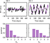 |
Fig. 1. Example of two simulated datasets, containing no planet signal (left) and two planet signals (right). Top: RV time series and random samples from the posterior predictive distribution. Bottom: Posterior distributions for Np. |
We performed the analysis of each dataset with kima, using default settings for the DNS algorithm. The priors used in the analysis are listed in Table B.1 of Appendix B. We note that the prior for the orbital period extends to two years, even though the time spans of the datasets are around one year. The DNS algorithm ran for 100 000 iterations, providing more than 10 000 effective posterior samples for each dataset.
The bottom panels of Fig. 1 show the resulting posteriors for the number of planets in the same two example datasets. On the left, Np = 0 has the highest posterior probability, pointing to no planet being detected, while in the second dataset, Np = 1 is the most probable value. Figure 2 shows the joint posterior for the planetary minimum mass and the orbital period, combining all values of Np, together with the three regions. The dataset shown on the right contained two simulated planets, within R2 and R3. Only one of these signals is detected, appearing as an over-density on the posterior inside R2.
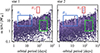 |
Fig. 2. Joint posteriors for the minimum mass and orbital period, shown as hexbin density plots, for the same example datasets as in Fig. 1. All samples with Np > 0 are shown. The three regions where the occurrence rates are estimated are shown as coloured boxes and labels. |
In Fig. 3, we show the occurrence rate estimates for the three regions, as obtained by combining the analysis of five, 25, and all 50 datasets. The plots show the assumed uniform prior and the resulting posterior distribution for each fR, as well as the true simulated values. It is clear that the analysis of only five datasets provides little information about the occurrence rates, even though it already assigns low posterior probability to fR = 0 and fR = 1 in R2, for example.
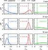 |
Fig. 3. Occurrence rate estimates for the three regions R1, R2, and R3, from the analysis of five, 25, and all 50 simulated datasets. The panels show the prior and posterior distributions (dotted and solid lines, respectively), and the true simulated values (vertical dashed lines). Each panel also shows the mean and standard deviation of the posterior distribution. The prior has a mean and a standard deviation of 0.5 and 0.28. |
Including more stars improves the precision of the posterior estimates, but differently for each region. This is discussed in more detail in Appendix C. Since none of the simulated datasets is sensitive to planets in R3, with long orbital periods and small masses, the estimate for the occurrence rate is uncertain, and the posterior is very close to the uniform prior.
4. Discussion
We presented a method for estimating the occurrence rate of planets in a given region of parameter space, from the analysis of RV data from several stars. Using samples from the posterior distributions of the individual analyses, we estimated the probability that at least one planet is present within a region limited in orbital period and planetary mass. This only required computing the fraction of the posterior samples that fall within the region and comparing it to the expected fraction from the prior.
Based on 50 simulated RV datasets, we inferred the occurrence rates for three regions, defined in such a way as to probe different RV detection sensitivities. In region R2, all simulated signals should be easy to detect, even with only ∼50 RV measurements (cf. the example in Fig. 1). On the other hand, none of the simulated time series are sensitive to planet signals in R3. Region R1 was chosen to represent an intermediate case, where some signals may be detected.
We recovered unbiased estimates of the occurrence rates for the three regions. As more stars were included, the posterior uncertainties decreased, and the estimates became more precise (see Fig. 3). For regions where the RV data were insensitive to planet signals, the posterior remained close to the prior, as expected.
This approach relies solely on existing posterior samples, does not require injection-recovery tests, and bypasses the need to define an explicit detection threshold. Moreover, the same set of posterior samples can be reused to estimate occurrence rates for different regions or stellar subsamples, offering a flexible and computationally efficient framework for population inference.
4.1. Caveats and assumptions
Listing the main assumptions of the proposed method may shed light on its limitations. Violations of these assumptions may lead to underestimated uncertainty or biased estimates of fR.
To write Eqs. (4) and (5), we assumed that the RV datasets for each star are independent (conditional on knowing fR). This may not be true in real RV surveys, because of either shared instrumental systematics or the presence of correlations within the stellar population under study. For example, the instrument used to measure the RVs may imprint a residual calibration error in all datasets, or the true planet occurrence may depend (strongly) on stellar parameters such as mass, metallicity, or age.
Our analyses assumed a simple white noise model, and the simulated datasets also only included white noise. Real RV data almost certainly contain other sources of noise, such as instrumental systematics or stellar activity signals. Fortunately, the method allows for more complex noise models to be used in the individual analyses, which may improve the sensitivity of the RV datasets to planets with lower mass, and mitigate the appearance of spurious signals.
We also assumed to have samples representative of the true posterior distributions, even in regions of low probability. In practice, care must be taken to ensure that the sampling algorithm is performed correctly across the parameter space (see Appendix D for some diagnostics).
4.2. Future work
Our method provides a simple way to make inferences about the exoplanet population. The natural next step is to apply it to real RV datasets from ongoing or historical surveys. We also plan to investigate how instrumental systematics and stellar activity influence the inferred occurrence rates, and to mitigate these effects by introducing more flexible noise models in the individual analyses. In addition, our approach can be extended to study planet multiplicity and other orbital characteristics, either by adapting the definition of the regions of interest or changing the statistical model (see Appendix D for details).
More generally, even though we focused on RV analysis in this work, similar approaches could be applied to transit and direct imaging surveys (see e.g. Foreman-Mackey et al. 2014; Bowler et al. 2020), enabling a unified view of the demographics of exoplanets across multiple detection techniques.
But see Appendix D for an alternative definition.
In particular, the individual analyses need not consider any specific region R where the occurrence rate is to be estimated.
Available at github.com/kima-org/kima.
Acknowledgments
We thank the anonymous referee for constructive feedback that improved this manuscript. This research was funded by the Swiss National Science Foundation (SNSF), grant numbers 200020, 205010.
References
- Baycroft, T. A., Triaud, A. H. M. J., Faria, J., Correia, A. C. M., & Standing, M. R. 2023, MNRAS, 521, 1871 [Google Scholar]
- Bonfils, X., Delfosse, X., Udry, S., et al. 2013a, A&A, 549, A109 [NASA ADS] [CrossRef] [EDP Sciences] [Google Scholar]
- Bonfils, X., Lo Curto, G., Correia, A. C. M., et al. 2013b, A&A, 556, A110 [NASA ADS] [CrossRef] [EDP Sciences] [Google Scholar]
- Bowler, B. P., Blunt, S. C., & Nielsen, E. L. 2020, AJ, 159, 63 [Google Scholar]
- Brewer, B. J. 2014, ArXiv e-prints [arXiv:1411.3921] [Google Scholar]
- Brewer, B. J., & Donovan, C. P. 2015, MNRAS, 448, 3206 [NASA ADS] [CrossRef] [Google Scholar]
- Brewer, B. J., Pártay, L. B., & Csányi, G. 2011, Stat. Comput., 21, 649 [Google Scholar]
- Buchner, J. 2023, Stat. Surv., 17, 169 [NASA ADS] [CrossRef] [Google Scholar]
- Cumming, A., Marcy, G. W., & Butler, R. P. 1999, ApJ, 526, 890 [Google Scholar]
- Elvira, V., Martino, L., & Robert, C. P. 2022, Int. Stat. Rev., 90, 525 [Google Scholar]
- Faria, J. P., Haywood, R. D., Brewer, B. J., et al. 2016, A&A, 588, A31 [NASA ADS] [CrossRef] [EDP Sciences] [Google Scholar]
- Faria, J. P., Santos, N. C., Figueira, P., & Brewer, B. J. 2018, JOSS, 3, 487 [NASA ADS] [CrossRef] [Google Scholar]
- Faria, J. P., Suárez Mascareño, A., Figueira, P., et al. 2022, A&A, 658, A115 [NASA ADS] [CrossRef] [EDP Sciences] [Google Scholar]
- Feroz, F., Hobson, M. P., & Bridges, M. 2009, MNRAS, 398, 1601 [NASA ADS] [CrossRef] [Google Scholar]
- Feroz, F., Balan, S. T., & Hobson, M. P. 2011, MNRAS, 415, 3462 [Google Scholar]
- Figueira, P., Faria, J. P., Silva, A. M., et al. 2025, A&A, 700, A174 [NASA ADS] [CrossRef] [EDP Sciences] [Google Scholar]
- Ford, E. B. 2005, AJ, 129, 1706 [Google Scholar]
- Foreman-Mackey, D., Hogg, D. W., & Morton, T. D. 2014, ApJ, 795, 64 [Google Scholar]
- Green, P. J. 1995, Biometrika, 82, 711 [CrossRef] [Google Scholar]
- Gregory, P. C. 2005, ApJ, 631, 1198 [NASA ADS] [CrossRef] [Google Scholar]
- Higson, E., Handley, W., Hobson, M., & Lasenby, A. 2019, Stat. Comput., 29, 891 [Google Scholar]
- Hogg, D. W., Myers, A. D., & Bovy, J. 2010, ApJ, 725, 2166 [Google Scholar]
- Howard, A. W., Marcy, G. W., Johnson, J. A., et al. 2010, Science, 330, 653 [Google Scholar]
- Jeffreys, H. 1939, Theory of Probability (Oxford: Oxford University Press) [Google Scholar]
- John, A. A., Collier Cameron, A., Faria, J. P., et al. 2023, MNRAS, 525, 1687 [Google Scholar]
- Kass, R. E., & Raftery, A. E. 1995, J. Am. Stat. Assoc., 90, 773 [Google Scholar]
- Lillo-Box, J., Figueira, P., Leleu, A., et al. 2020, A&A, 642, A121 [NASA ADS] [CrossRef] [EDP Sciences] [Google Scholar]
- Mayor, M., Marmier, M., Lovis, C., et al. 2011, ArXiv e-prints [arXiv:1109.2497] [Google Scholar]
- Rosenthal, L. J., Fulton, B. J., Hirsch, L. A., et al. 2021, ApJS, 255, 8 [NASA ADS] [CrossRef] [Google Scholar]
- Skilling, J. 2004, AIP Conf. Proc., 735, 395 [Google Scholar]
- Skilling, J. 2006, Bayesian Anal., 1, 833 [Google Scholar]
- Standing, M. R., Triaud, A. H. M. J., Faria, J. P., et al. 2022, MNRAS, 511, 3571 [NASA ADS] [CrossRef] [Google Scholar]
- Tuomi, M., Jones, H. R., Barnes, J. R., Anglada-Escudé, G., & Jenkins, J. S. 2014, MNRAS, 441, 1545 [NASA ADS] [CrossRef] [Google Scholar]
- Wright, J. T., & Gaudi, B. S. 2013, in Planets, Stars and Stellar Systems, eds. T. D. Oswalt, L. M. French, & P. Kalas (Dordrecht: Springer), 489 [Google Scholar]
- Zhu, W. 2019, ApJ, 873, 8 [NASA ADS] [CrossRef] [Google Scholar]
Appendix A: Estimating π(𝒫)
The assumed priors for the model parameters define the prior distribution for the event 𝒫 for each star: a Bernoulli distribution with probability f0 (see Eq. 8). In the uninteresting limit where the priors exclude the region of interest, this probability is zero and the proposed method to estimate the occurrence rate is ill-defined. In other cases, the prior probability can be computed from the separable priors for the orbital period πP, the semi-amplitude πK, the eccentricity πe, and the number of planets πNp.
In practice, we estimate f0 using Monte Carlo: we draw a large number of random samples from πP, πK, and πe, calculate the planet mass for each sample using the stellar mass, and count the number of samples that fall within the region of interest. If the cumulative distribution function of πP is known, the random sampling can be made more efficient (and lower variance) by only sampling periods within the region. Denoting the fraction of samples falling within the region as F, we then calculate
 (A.1)
(A.1)
where Npmax is the maximum value of Np (set to 5 in our analyses, see Table B.1). This expression accounts for the “at least one” constraint on the definition of 𝒫. The calculation of f0 needs to be repeated for each star with the appropriate value for the stellar mass. With modern hardware, obtaining the random samples and calculating Eq. (A.1) can be achieved in about one second.
In Fig. A.1, we sketch this calculation, showing several thousand random samples from the prior distribution (for Np = 1) in the plane of orbital period and planet minimum mass, together with the three regions R1, R2, and R3 defined in the main text. For our choice of priors, the fraction of samples that fall within the regions and the corresponding values of f0 are
-
F ≈ 0.142 and f0 ≈ 0.295 for R1
-
F ≈ 0.022 and f0 ≈ 0.053 for R2
-
F ≈ 0.029 and f0 ≈ 0.072 for R3
as obtained from 10,000,000 prior samples.
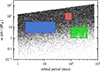 |
Fig. A.1. Procedure to estimate f0 using random samples from the prior distribution that fall inside each region of interest. |
If the prior distribution is assigned directly to planet mass instead of RV semi-amplitude, there may be analytical expressions for all cumulative distributions, allowing for a calculation of f0 that does not rely on Monte Carlo.
Appendix B: Model parameters and priors
This appendix details the parameters and prior distributions used in the RV analysis. We parametrise each of the Np Keplerian functions with the orbital period P, the semi-amplitude K, the orbital eccentricity e, the argument of pericentre ω, and the mean anomaly at the epoch M0. The reference epoch is set to the time of the first observation. The systemic velocity is denoted as vsys and is fixed to zero for simplicity. A jitter parameter σJ is used to account for otherwise unmodelled white noise.
Each dataset consists of N observations containing the times ti, the radial velocity measurements viobs, and the associated uncertainties σi. We further define the model radial velocities, vi, as deterministic functions of the orbital parameters and vsys. The connections between all the parameters are shown in Fig. B.1 as a probabilistic graphical model.
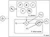 |
Fig. B.1. Probabilistic graphical model for the RV analysis. An arrow between two nodes indicates the direction of conditional dependence. The circled nodes are parameters of the model, whose joint distribution is sampled. The filled node represents the observed RVs. The ti and σi nodes are assumed given and thus fixed, while the vi are deterministic functions of other nodes. The variables inside the boxes are repeated a given number of times. The dashed line connecting fR indicates the importance sampling scheme used to estimate the posterior for this parameter. |
Prior distributions for each parameter are listed in Table B.1. Note that these same priors were used for sampling the orbital parameters of the simulated planets, while ensuring the values fell within each region of interest.
Prior distributions used in the RV analysis.
Appendix C: Posterior uncertainties
The usual method to estimate planet occurrence rates from RV surveys relies on binomial statistics. That is, it is assumed that the number of planets detected, k, follows a binomial distribution with parameters S and fR, using our notation. To account for the different sensitivity of each star, the average completeness within the region R is used to calculate an “effective” number of stars, Seff, that replaces S in the binomial probability.
Even if not explicitly stated, the inference for fR within this context is usually based on the beta-binomial distribution: a beta distribution (of which the uniform distribution is a special case) is often assumed as the prior for fR. The beta is a conjugate prior to the binomial, so the posterior distribution for fR is also a beta distribution, with parameters

where the +1 factors come from the uniform prior.
The standard deviation of the posterior for fR is maximised if there are ⌊S/2⌋ or ⌈S/2⌉ detections, it is minimised if there are zero or S detections, and depends on the true value of fR within this range. This is shown in Fig. C.1, as a function of S. As we increase the number of stars in the sample, the posterior uncertainty for fR will stay within this range. If only Seff stars have enough sensitivity to detect a planet, the uncertainty in the posterior is larger. Figure C.1 shows a dashed curve for the case where Seff = S/2 (completeness of 50%).
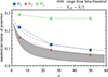 |
Fig. C.1. Standard deviation of the posterior distribution for fR as a function of the number of stars in the sample S. |
Overplotting the standard deviations of the inferred posterior distributions for fR using our method (see values listed in Fig. 3) shows good agreement with the beta-binomial results. We see two sources of uncertainty being reflected in the posterior: from the number of stars included in the analysis and from the sensitivity of each star’s RV time series.
As expected, each of the three regions we studied is affected differently by these uncertainties. All RV datasets are sensitive to planets in R2, so the posterior uncertainty comes only from the limited number of stars in the sample. For R1, only a fraction of the stars are sensitive to planets with these orbital periods and masses, so the posterior uncertainty is larger, and comparable to a completeness fraction of 50%. Inference in region R3 is mostly controlled by the prior.
In summary, the uncertainty in our inferred occurrence rates is compatible with other methods, but our approach completely avoids having to determine k and the survey completeness.
Appendix D: Generalisations and diagnostics
In section 2.3, the planet occurrence rate was defined as the fraction of stars with at least one planet within a region of parameter space. An alternative definition could be the average number of planets per star within that region (e.g. Zhu 2019). With some modifications, our method can be used to estimate this quantity.
We define the event “there are np planets with parameters in a given region”, denoted by np itself (not to be confused with Np), which takes non-negative integer values. For each star, we assume this event follows a Poisson distribution with rate parameter equal to the average number of planets per star within the region, here denoted as λR:
 (D.1)
(D.1)
The priors used in the individual analyses again define a prior probability for np, but now it is not within the same distribution family. The original priors were defined for the total number of planets in the system, Np. The prior probability that np out of Np planets are within R is given by a binomial distribution. After marginalising out Np, we obtain:
 (D.2)
(D.2)
where F is the probability of one planet being within R, which was estimated using Monte Carlo (see Appendix A). The upper limit in the sum is set by the maximum value for Np in the prior.
The ratio p(λR; np)/π(F; np) can then be used to compute the likelihood, analogously to Eq. (7) but using np, jk as the number of planets in R for each posterior sample, and thus the posterior for λR can be evaluated after defining a prior p(λR). As before, a uniform distribution, from 0 to 5, may be a suitable choice.
Some caveats are worth mentioning. The Poisson assumption (D.1) implies that different planets around the same star occur independently, which is likely not true. Moreover, the original prior π(F; np) and the new prior p(λR; np) may be very different for some values of λR, leading to high variance in the importance sampling approximation (Eq. 6).
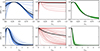 |
Fig. D.1. Ratio of effective sample size (ESS) in the importance sampling approximation to the total number of posterior samples vs the fraction of stars with planets fR (top) and the average number of planets per star λR (bottom), for each star and each box. The thick black curves show the mean ratio across all stars. |
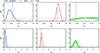 |
Fig. D.2. Results from bootstrap resampling of the posterior samples for the three regions R1, R2, R3, and from the analysis of all 50 simulated datasets. Top: Posterior distributions for the fraction of stars with planets. Bottom: Posteriors for the average number of planets per star. The lines are the same as in Fig. 3. Note that the true values of fR and λR are the same due to the way the simulated datasets were generated. |
A useful diagnostic when using importance sampling is the effective sample size (ESS), which can be computed from the ratio of the two priors, usually called the importance weight (e.g. Elvira et al. 2022). The ESS essentially quantifies how many of the posterior samples, obtained based on π(f0; 𝒫) or π(F; np), have substantial weight under the new priors p(fR; 𝒫) or p(λR; np). We estimate the ESS for each simulated star as
 (D.3)
(D.3)
with the weights defined as
 (D.4)
(D.4)
Figure D.1 shows the ratio of the ESS to the total number of posterior samples for each star and region, as a function of fR and λR. In the case of fR, the ESS is above 50% of the number of posterior samples, except for values close to 1 for R1 and above 0.25 for R3. Therefore, the importance sampling approximation is less accurate in these cases. For R1, this has a small impact on the results since the posterior for fR peaks at lower values. The ESS is in general smaller for λR, especially for R3, due to the larger mismatch between the original and new priors.
Another way to diagnose the results is to perform bootstrap resampling, by randomly shuffling (with replacement) the posterior samples for each star and recomputing the occurrence rate posteriors. An example of this is shown in Fig. D.2, which plots the posteriors for fR and λR for each region, obtained from 30 resampling iterations. The posteriors show little variation for R1 and R2, but the variance and bias are higher for R3.
Finally, we note that a perhaps more natural generalisation of the method would be to estimate the individual probabilities for np = 0, np = 1, and so on, while maybe collapsing all values above a certain number into one bin (e.g. np ≥ 2). These individual probabilities could be modelled with a Dirichlet distribution, allowing for a larger flexibility than the Poisson, with few additional parameters. Such a parametrisation might also be more easily compared to empirical probabilities provided by planet formation models.
All Tables
All Figures
|
Fig. 1. Example of two simulated datasets, containing no planet signal (left) and two planet signals (right). Top: RV time series and random samples from the posterior predictive distribution. Bottom: Posterior distributions for Np. |
| In the text | |
|
Fig. 2. Joint posteriors for the minimum mass and orbital period, shown as hexbin density plots, for the same example datasets as in Fig. 1. All samples with Np > 0 are shown. The three regions where the occurrence rates are estimated are shown as coloured boxes and labels. |
| In the text | |
|
Fig. 3. Occurrence rate estimates for the three regions R1, R2, and R3, from the analysis of five, 25, and all 50 simulated datasets. The panels show the prior and posterior distributions (dotted and solid lines, respectively), and the true simulated values (vertical dashed lines). Each panel also shows the mean and standard deviation of the posterior distribution. The prior has a mean and a standard deviation of 0.5 and 0.28. |
| In the text | |
|
Fig. A.1. Procedure to estimate f0 using random samples from the prior distribution that fall inside each region of interest. |
| In the text | |
|
Fig. B.1. Probabilistic graphical model for the RV analysis. An arrow between two nodes indicates the direction of conditional dependence. The circled nodes are parameters of the model, whose joint distribution is sampled. The filled node represents the observed RVs. The ti and σi nodes are assumed given and thus fixed, while the vi are deterministic functions of other nodes. The variables inside the boxes are repeated a given number of times. The dashed line connecting fR indicates the importance sampling scheme used to estimate the posterior for this parameter. |
| In the text | |
|
Fig. C.1. Standard deviation of the posterior distribution for fR as a function of the number of stars in the sample S. |
| In the text | |
|
Fig. D.1. Ratio of effective sample size (ESS) in the importance sampling approximation to the total number of posterior samples vs the fraction of stars with planets fR (top) and the average number of planets per star λR (bottom), for each star and each box. The thick black curves show the mean ratio across all stars. |
| In the text | |
|
Fig. D.2. Results from bootstrap resampling of the posterior samples for the three regions R1, R2, R3, and from the analysis of all 50 simulated datasets. Top: Posterior distributions for the fraction of stars with planets. Bottom: Posteriors for the average number of planets per star. The lines are the same as in Fig. 3. Note that the true values of fR and λR are the same due to the way the simulated datasets were generated. |
| In the text | |
Current usage metrics show cumulative count of Article Views (full-text article views including HTML views, PDF and ePub downloads, according to the available data) and Abstracts Views on Vision4Press platform.
Data correspond to usage on the plateform after 2015. The current usage metrics is available 48-96 hours after online publication and is updated daily on week days.
Initial download of the metrics may take a while.