| Issue |
A&A
Volume 705, January 2026
|
|
|---|---|---|
| Article Number | A182 | |
| Number of page(s) | 28 | |
| Section | Interstellar and circumstellar matter | |
| DOI | https://doi.org/10.1051/0004-6361/202555717 | |
| Published online | 22 January 2026 | |
The MATISSE view of the inner region of the RY Tau protoplanetary disk★
1
Institut für Theoretische Physik und Astrophysik, Christian-Albrechts-Universität zu Kiel,
Leibnizstraße 15,
24118
Kiel,
Germany
2
Konkoly Observatory, Research Centre for Astronomy and Earth Sciences, HUN-REN,
Konkoly Thege Miklós út 15–17.,
1121
Budapest,
Hungary
3
Laboratoire Lagrange, Université Côte d’Azur, Observatoire de la Côte d’Azur, CNRS, Boulevard de l’Observatoire,
CS
34229, 06304
Nice Cedex 4,
France
4
Univ. Grenoble Alpes, CNRS, IPAG,
38000
Grenoble,
France
5
NOVA Optical IR Instrumentation Group at ASTRON,
The Netherlands
6
Max-Planck-Institut für Astronomie,
Königstuhl 17,
69117
Heidelberg,
Germany
7
NASA Goddard Space Flight Center, Astrophysics Division,
Greenbelt,
MD
20771,
USA
8
Anton Pannekoek Institute for Astronomy, University of Amsterdam,
Science Park 904,
1090
GE
Amsterdam,
The Netherlands
9
European Southern Observatory,
Karl-Schwarzschild-Str. 2,
85748
Garching,
Germany
10
Max-Planck-Institut für Radioastronomie,
Auf dem Hügel 69,
53121
Bonn,
Germany
11
Leiden Observatory, Leiden University,
PO Box 9513,
2300
RA
Leiden,
The Netherlands
12
Steward Observatory, Department of Astronomy, University of Arizona,
Tucson,
AZ
85721,
USA
13
Physikalisches Institut, Universität zu Köln,
Zülpicher Str. 77,
Cologne
50937,
Germany
14
School of Physics & Astronomy, University of Southampton,
University Road,
Southampton
SO17 1BJ,
UK
15
European Southern Observatory, Alonso de Córdova,
3107
Vitacura, Santiago,
Chile
16
AIM, CEA, CNRS, Université Paris-Saclay, Université Paris Diderot, Sorbonne Paris Cité,
91191
Gif-sur-Yvette,
France
★★ Corresponding author: This email address is being protected from spambots. You need JavaScript enabled to view it.
Received:
28
May
2025
Accepted:
27
October
2025
Abstract
Context. The physical conditions and processes taking place in the innermost regions of protoplanetary disks are essential for planet formation and general disk evolution. In this context, we study the T-Tauri type young stellar object RY Tau, which exhibits a dust-depleted inner cavity characteristic of a transition disk.
Aims. The goal of this study is to analyze spectrally resolved interferometric observations in the L, M, and N bands of the RY Tau protoplanetary disk obtained with MATISSE. We aim to provide constraints on the spatial distribution and mineralogy of dust in the inner few astronomical units by producing synthetic observations fitting the interferometric observables.
Methods. We employed a 2D temperature gradient disk model to estimate the orientation of the inner disk. Successively, we analyzed the chemical composition of silicates depending on spatial region in the disk. Finally, we sampled the parameter space of a viscous accretion disk model via Monte Carlo radiative transfer simulations to investigate the actual 3D dust density distribution of RY Tau.
Results. We constrained the orientation of the inner disk of RY Tau, finding no evidence of significant misalignment with respect to its outer disk. We identified several silicate species commonly found in protoplanetary disks and observed a depletion of amorphous dust grains toward the central protostar. By simultaneously considering the observed visibilities and the spectral energy distribution (SED), we found that an accretion disk and an optically thin envelope enshrouding the protostar fits the observations best. Radiative transfer simulations show that hot dust close to the protostar and in the line of sight (LOS) to the observer, either in the uppermost disk layers of a strongly flared disk or in a dusty envelope, is necessary to model the observations. The shadow cast by a dense innermost disk midplane on the dust further out explains the observed closure phases in the L band and (to some extent) in the M band. However, the closure phases in the N band are underestimated by our model, hinting at an additional asymmetry in the flux density distribution that is not visible at shorter wavelengths.
Key words: astrochemistry / radiative transfer / instrumentation: interferometers / protoplanetary disks / stars: individual: RY Tau / stars: variables: T Tauri, Herbig Ae/Be
Based on observations collected at the European Organisation for Astronomical Research in the Southern Hemisphere with the VLTI-MATISSE instrument under ESO programmes 106.21Q8.006 and 106.21Q8.002.
© The Authors 2026
 Open Access article, published by EDP Sciences, under the terms of the Creative Commons Attribution License (https://creativecommons.org/licenses/by/4.0), which permits unrestricted use, distribution, and reproduction in any medium, provided the original work is properly cited.
This article is published in open access under the Subscribe to Open model. This email address is being protected from spambots. You need JavaScript enabled to view it. to support open access publication.
1 Introduction
Observing young stellar objects (YSOs) in active star forming regions is crucial to testing theoretical models of the star and planet formation processes. Stars form through the gravitational collapse of molecular clouds with angular momentum conservation, leading to the formation of an accretion disk (e.g., Williams & Cieza 2011). These circumstellar disks are made up of gas and dust, extending across several hundred astronomical units (au) and they are the progenitors of planetary systems with planet formation taking place within them (e.g., Keppler et al. 2018). YSOs in different evolutionary stages classified by their spectral energy distribution (SED; Lada 1987) have been observed by direct imaging and spectroscopic measurements on large scales (e.g., Smith et al. 2005; Espaillat et al. 2011; Garufi et al. 2024), revealing a diverse population of different sizes, shapes, and dust compositions. In recent years, infrared (IR) long-baseline interferometric observations have provided additional insights into the evolution of protoplanetary disks (e.g., van Boekel et al. 2004; Monnier et al. 2006; Weigelt et al. 2011; Menu et al. 2015; Brunngräber et al. 2016; Lazareff et al. 2017; Varga et al. 2018; Kobus et al. 2020; Varga et al. 2021; Hofmann et al. 2022; Varga et al. 2024), probing their innermost regions comparable in size to the inner Solar System harboring the terrestrial planets.
The physical processes driving planet formation and the transition from the dispersal of the natal envelope to the various evolutionary stages of protoplanetary disks are not yet fully understood, but they can be extensively described with various theoretical models. A depletion of dust grains in the innermost disk regions is observed in a small population of YSOs (Calvet et al. 2002; Brown et al. 2007; Andrews et al. 2011; Francis & van der Marel 2020), indicating a short-lived transition disk state. Selected explanations of this phenomenon include extensive particle growth (Dullemond & Dominik 2005), photoevaporation driven disk winds (Alexander et al. 2006), the gravitational impact of companions of the embedded YSO (Lin & Papaloizou 1979; Penzlin et al. 2024), or dead zones induced by embedded planets in the outer disks (Regály et al. 2012; Kley & Nelson 2012).
An exemplary, extensively studied transition disk is that of RY Tau, which is an intermediate mass classical T-Tauri star (CTTS) (St-Onge & Bastien 2008; Petrov et al. 2019; Valegård et al. 2022) in the Taurus-Auriga Molecular Cloud (Kenyon et al. 1994) with an estimated age of 4 Myr (Valegård et al. 2021). The SED is characteristic for a Class II object (Lada 1987; Garufi et al. 2018, 2019, 2024) and an inclined circumstellar disk is detected in the (sub-)millimeter wavelength range (Isella et al. 2010; Long et al. 2019; Harrison et al. 2024), which is typical for a CTTS. These observations reveal an inner dust cavity with a radius of 27 au and ring-like structures on larger scales, possibly caused by ongoing planet formation (Francis & van der Marel 2020).
Observations in the optical and near-infrared (NIR) show that the protostar of RY Tau is enshrouded by dust (Nakajima & Golimowski 1995; Takami et al. 2013; Davies et al. 2020; Takami et al. 2023), which can be attributed to the remnants of the natal envelope (Garufi et al. 2019) or a disk wind (Babina et al. 2016; Valegård et al. 2022; Sauty et al. 2022; Meskini et al. 2024). RY Tau exhibits UX Ori-type behavior, that is, strong variability in the visible wavelength range (Petrov et al. 1999). The variability is accounted for by obstruction of the host star by a dusty environment (Babina et al. 2016), which is a common phenomenon among YSOs (Kobus et al. 2020). Petrov et al. (2021) reported anticyclic variations of gas infall and outflow, which could be caused by magnetohydrodynamic processes or a close-in planet interacting with the accretion disk. A bipolar jet (HH938) is observed in X-ray (Skinner et al. 2016), far-ultraviolet (FUV; Skinner et al. 2018), visible, and NIR (St-Onge & Bastien 2008; Garufi et al. 2019; Takami et al. 2023) wavelengths.
Mid-infrared (MIR) observations obtained with the Spitzer Space Telescope (Espaillat et al. 2011) show a strong silicate emission feature at a wavelength of approximately 10 μm. The FIR to submillimeter (submm) photometry is provided by Herschel Space Observatory observations (Ribas et al. 2017). Interferometric observations using the MID-infrared Interferometric instrument (MIDI; Leinert et al. 2003) in the N band have provided the first insights into the circumstellar dust composition in the innermost disk regions, revealing an increase in crystalline silicates compared to amorphous dust toward the central protostar. Schegerer et al. (2008) additionally found that a radiative transfer model of an accretion disk in combination with an envelope fits the SED and visibilities of two baselines in the N band well.
Interferometric observations of RY Tau in the K band (2.0–2.4 μm) were collected using the Center for High Angular Resolution Astronomy (CHARA) array and the GRAVITY instrument at the VLTI (GRAVITY Collaboration 2021). These observations provide evidence of an inner disk rim shaped by sublimation, and occultation of the central protostar of RY Tau by close-in dust in the LOS to the observer (Davies et al. 2020). The characteristic sizes (i.e., the half-flux radii) of RY Tau in the NIR and MIR are 2.54 mas in the K band (GRAVITY Collaboration 2021) and 8.0 mas in the N band (Varga et al. 2018).
In this work, we present the first interferometric observations of RY Tau covering the L (3.2–3.9 μm), M (4.5–5.0 μm) and N (8–13 μm) bands simultaneously. The data were collected using the Multi AperTure mid-Infrared SpectroScopic Experiment (MATISSE; Lopez et al. 2022) at the Very Large Telescope Interferometer (VLTI). The goal of this study is to present constraints on the spatial distribution and mineralogy of the dust in the inner few astronomical units around the central protostar of RY Tau. To this end, we employ a model-driven approach to produce synthetic observations that fit the spectrally resolved measurements by MATISSE presented in Sect. 2. We introduce the basic methods used in this work in Sect. 3. We present a 2D semi-physical, radially symmetric disk model with a simple temperature prescription to constrain the inner disk orientation in Sect. 4. On the basis of the estimated orientation of the inner disk, the radial dependence of the silicate composition of the circumstellar dust is investigated in Sect. 5. Finally, a large set of radiative transfer simulation results is presented and analyzed in Sect. 6 to provide constraints on the spatial dust distribution in the circumstellar vicinity of RY Tau, which is the main goal of this work.
2 MATISSE observations and data reduction
RY Tau was observed with MATISSE (Lopez et al. 2022) in January 2021 in the frame of a Guaranteed Time Observing (GTO) program for surveying YSOs, providing the first simultaneous L-, M-, and N-band interferometric observations. To increase the u-v coverage in the L band, additional observations were performed after 16 days. These short times between observations, compared to periods of strong changes in activity on a timescale of ~yr (e.g., Petrov et al. 2019), allowed us to model a consistent YSO state without having to take temporal variability into account. We note, however, that Petrov et al. (2021) reported variation of radial velocities accompanied by visible light magnitude changes ~0.5 mag with a period of 22 d. Nevertheless, we take the additional L-band observations on January 23 into account in our modeling, assuming that the dusty environment around the protostar does not change enough to have a significant impact on the observed visibilities. An overview of the observations analyzed in this work is given in Table 1. The spectral resolutions are 31.5 for LOW-LM, 499 for MED-LM, and 218 for HIGH-N spectral modes, respectively (Lopez et al. 2022). The auxiliary telescopes (ATs) observations were collected in the “medium” configuration with the ATs placed at the stations given in Table 1. In total, we collected data on six baselines in the L, M and N band using the unit telescopes (UTs) and, additionally, on twelve baselines in the L band using the ATs. The u-v coordinates of the baselines are shown in Fig. 4.
The data reduction was performed as described in Millour et al. (2016) with the standard MATISSE data reduction pipeline DRS version given in Table 1. We applied post-processing, including flux calibration and the averaging of exposures with the MATISSE Python tools1, and with our own Python scripts as well. More details on the data processing workflow can be found in Sect. 3.1 of Varga et al. (2021). To fit the 2D and 3D disk models (see Sects. 4 and 6) to the data, we reduced the spectral resolution of the observations by weighted averaging of the measured values and simple averaging of the errors of the observables V2 and ϕcp over wavelength bins. Thanks to this simple averaging of the errors, we ensured that we could remain conservative and avoid underestimating any possible systematic uncertainties. The wavelength bin width, Δλ, was chosen depending on the band; Δλ(L, M) = 0.05 μm, Δλ(N) = 0.1 μm. The spectral averaging of the data yields a common wavelength grid for all baselines per spectral band on which the modeled observables were computed. This approach reduces the computational cost of the modeling significantly, compared to modeling the observables at the full spectral resolution.
As the quality of the measured data degrades toward the short wavelengths of the L band, we used the data in the 3.5–3.9 μm range only. For the same reason, we considered measurements at 4.5–5.2 μm in the M band and 8.1–13.0 μm in the N band.
The measured squared visibilities, V2, closure phases, ϕcp, and correlated fluxes, Fcorr, in the N band are shown in Fig. 1. The slope of the measured squared visibilities indicate that the apparent size of RY Tau increases with wavelength, which is typical for a protoplanetary disk in the NIR and MIR. The closure phases are nonzero for most baselines in the L and M band and large closure phases are observed in the N band, which indicates an asymmetric intensity distribution, with a stronger asymmetry at longer wavelengths. The correlated fluxes in the N band show a prominent silicate emission feature, which changes its shape with baseline length.
MATISSE observations of RY Tau analyzed in this paper.
3 Methods
The observations shown in Fig. 1 are used to constrain the spatial distribution and chemical composition of the dust in the circumstellar environment by fitting different models to the measured data. As a quality criterion of how well a given model reproduces the observations the reduced, χ2, expressed as
![Mathematical equation: $\[\chi_{\mathrm{red}}^2(q)=\frac{1}{N_{\mathrm{data}}-N_{\mathrm{free}}} \sum_i^{N_{\mathrm{data}}} \frac{\left(q_i-m_{q; i}\right)^2}{\sigma_{q_i}^2},\]$](/articles/aa/full_html/2026/01/aa55717-25/aa55717-25-eq1.png) (1)
(1)
is computed from the measured quantity, qi ± σqi, and the modeled value, mq;i, for the number of data points, Ndata, and the number of free parameters, Nfree, of the model (e.g., Hogg et al. 2010). A statistically solid approach is to sample the parameter space of a given model via the Markov Chain Monte Carlo (MCMC) algorithm (Goodman & Weare 2010), which was employed to fit a 2D temperature gradient disk model (see Sect. 4) and a 1D single temperature model (see Sect. 5) to the observations. The fits are performed using the Python implementation emcee (Foreman-Mackey et al. 2013). The resulting best-fit value is the median of the posterior probability density distribution of the fit parameter. The corresponding negative and positive errors on the best-fit value are taken as the 16% and 84% percentiles (corresponding to ∓1σ error bars of a normal distribution) of the distribution, respectively.
In Sect. 6, we describe how we modeled the observations by simulating the appearance of a 3D dust density distribution in the circumstellar environment illuminated by the central protostar of RY Tau. This is achieved with Monte Carlo Radiative Transfer (MCRT) simulations performed with POLARIS2 (Reissl et al. 2016, 2018). Flux density maps are simulated by computing the dust temperature distribution self-consistently (Bjorkman & Wood 2001) and successively deriving the thermal emission of the dust arriving at the detector via numerical integration along rays. Scattering of stellar light is taken into account employing the Monte Carlo technique (Wolf et al. 1999) optimized by utilizing peel-off photon packages (Yusef-Zadeh et al. 1984) and enforcing first scattering (Mattila 1970). Self-scattering of photons emitted by the dust off the dust is neglected as experimental simulations showed that it would have little influence on synthetic MATISSE observations of RY Tau. The computational cost of a single MCRT simulation is high, which renders MCMC sampling unfeasible. We resorted to a brute force exploration of the parameter space on a coarse grid of free parameter values to find a combination of parameters that would fit the observables best with respect to chosen parameter value resolution and range. If necessary, the coarse grid was successively refined in interesting regions of the parameter space. The comparison of the synthetic observables produced by the 2D and 3D disk models to the interferometric measurements of visibilities, V2, and closure phases, ϕcp, requires us to compute them from the flux density maps, which is achieved using the Python package galario (Tazzari et al. 2018).
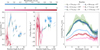 |
Fig. 1 Overview of the MATISSE observations of RY Tau listed in Table 1. The corresponding u–v coordinates are shown in Fig. 4. Left panel: Squared visibilities, V2, over projected baseline length Bp (pink/red: 8–13 μm wavelengths; blue/green: 3.5–5.2 μm wavelengths; see color bars). Middle panel: Measured closure phases, ϕcp, over the longest projected baseline length in the telescope triplet, Bp;max. Right panel: Correlated fluxes, Fcorr, and corresponding projected baseline length, Bp, and orientation, ϕB, in the N band. |
4 Estimation of disk orientation
Constraining the inner disk orientation defined by the inclination, ι, and position angle, PA, is crucial for the further analysis of the circumstellar dust environment of RY Tau. The position angle, PA, is defined as the angle of the disk major axis in the image plane measured from north to east. Atacama Large Millimeter/submillimeter Array (ALMA) observations provide a reliable value for the disk orientation on large scales, resulting in ιALMA = (65.0 ± 0.1)° and PAALMA = (23.1 ± 0.1)° (Long et al. 2019); these values were adopted by Davies et al. (2020) for the inner disk orientation. In this study, we chose to estimate the inner disk orientation independently, as Bohn et al. (2022) and Villenave et al. (2024) reported that a tilted inner disk might be a common phenomenon among YSOs.
4.1 2D star and disk model
To constrain the inner disk orientation, we adopted the semi-physical model proposed by Menu et al. (2015), assuming that the dominating radiation in the MIR originates from an optically thin surface layer of an accretion disk with constant optical depth, τν. Neglecting scattered light and optical depth effects, the disk intensity, Idisk:ν, as a function of the radial distance, r, from the central object is given by
![Mathematical equation: $\[I_{\mathrm{disk}; \nu}=\tau_\nu B_\nu(T(r)) \propto B_\nu~(T(r)),\]$](/articles/aa/full_html/2026/01/aa55717-25/aa55717-25-eq2.png) (2)
(2)
with Bν denoting the Planck function and assuming a radial temperature gradient following
![Mathematical equation: $\[T(r)=T_{\mathrm{in}}\left(\frac{r}{R_{\mathrm{in}}}\right)^{-q},\]$](/articles/aa/full_html/2026/01/aa55717-25/aa55717-25-eq3.png) (3)
(3)
as used by Menu et al. (2015) and Varga et al. (2017, 2018). The inner temperature Tin can be related to the inner radius Rin of the disk via
![Mathematical equation: $\[R_{\mathrm{in}}=\sqrt{\frac{L_{\star}}{4 \pi \sigma_{\mathrm{SB}} T_{\mathrm{in}}^4}},\]$](/articles/aa/full_html/2026/01/aa55717-25/aa55717-25-eq4.png) (4)
(4)
assuming an optically thick inner rim emitting as a blackbody (e.g., Dullemond & Monnier 2010) and neglecting the backwarming effect due to thermal emission of the dust (e.g., Bensberg & Wolf 2022). We note that this model is a strong simplification of the expected flared accretion disk with an optically thick disk midplane and an optically thin surface layer. However, it serves the purpose of estimating the inner disk orientation, which is then used to investigate the appearance of an illuminated 3D dust density distribution via MCRT simulations in Sect. 6.
The simple thin disk model needs to be completed by a stellar model in order to derive synthetic visibilities. In our study, we adopted the stellar properties used by Davies et al. (2020) given in Table 23. The stellar radius, R⋆, was derived applying the Stefan-Boltzmann law. Assuming the central protostar as a blackbody emitter, the disk-to-star flux ratio, f°(λ), was computed from total flux measurements. As the visibilities are a measure of contrast and do not include information on the absolute flux density values, it is expedient to norm the flux density of the central object to one and scale the disk intensity (see Eq. (2)) via the disk-to-star flux ratio. Interstellar extinction is taken into account adopting the extinction law proposed by Cardelli et al. (1989) using the Python package extinction4 with the visual magnitude, AV, given in Table 2. The resulting disk-to-star flux ratio is shown in Fig. 2. We note that the protostar contributes ≳10% to the total flux in L and M bands, while it contributes very slightly in the N band.
Stellar parameter used in this work.
4.2 Results
The disk orientation was constrained by fitting the free parameters of the model described in Sect. 4.1; namely, the inclination, ι, position angle, PA, and the disk temperature gradient exponent, q. The sublimation temperature of the dust was set to Tin = 1500 K, which is a common choice for cosmic dust consisting mainly of silicates (Vaidya et al. 2009; Menu et al. 2015; Hofmann et al. 2022). The best-fit parameters are listed in Table 3 and the modeled visibilities and normalized flux density maps at selected wavelengths are shown in Fig. A.1. The resulting ![Mathematical equation: $\[\chi_{\text {red}}^{2}\]$](/articles/aa/full_html/2026/01/aa55717-25/aa55717-25-eq5.png) > 10 indicates that the adopted model is not able to reproduce the observed visibilities well, which is also apparent in Fig. A.1. To improve the fit, the inner radius of the disk Rin, which is related to the sublimation temperature of the dust Tin via Eq. (4), was treated as free parameter. This choice was justified, as the dust sublimation temperature varies for different grain materials and silicate grains and is predicted that it may reach values of up to 2100 K (Duschl et al. 1996). Consequently, the inner rim radius is fitted indirectly via the sublimation temperature. The best-fit parameters are given in Table 3 and the comparison of modeled and measured visibilities is shown in Fig. 3. Compared to the model with a fixed sublimation temperature, Tin = 1500 K, a significantly reduced
> 10 indicates that the adopted model is not able to reproduce the observed visibilities well, which is also apparent in Fig. A.1. To improve the fit, the inner radius of the disk Rin, which is related to the sublimation temperature of the dust Tin via Eq. (4), was treated as free parameter. This choice was justified, as the dust sublimation temperature varies for different grain materials and silicate grains and is predicted that it may reach values of up to 2100 K (Duschl et al. 1996). Consequently, the inner rim radius is fitted indirectly via the sublimation temperature. The best-fit parameters are given in Table 3 and the comparison of modeled and measured visibilities is shown in Fig. 3. Compared to the model with a fixed sublimation temperature, Tin = 1500 K, a significantly reduced ![Mathematical equation: $\[\chi_{\text {red}}^{2}\]$](/articles/aa/full_html/2026/01/aa55717-25/aa55717-25-eq6.png) is achieved. As this could be the effect of overfitting, the Akaike information criterion, AIC (Akaike 1974), was computed, and we found that its lower value for the model with sublimation temperature as a free parameter (see Table 3) excludes this possibility.
is achieved. As this could be the effect of overfitting, the Akaike information criterion, AIC (Akaike 1974), was computed, and we found that its lower value for the model with sublimation temperature as a free parameter (see Table 3) excludes this possibility.
Taking into account the simplicity of the model (2D geometry, radial symmetry, and four free parameters), the synthetic visibilities match the observed visibilities well. The fit between model and observations is especially good in the N band, while in the L and M bands, the visibilities tend to be underestimated for longer baselines and overestimated for shorter baselines. This indicates that the emission in the shorter wavelength range of the MIR lacks some component which adds flux from the innermost part of the disk. Surprisingly, our best-fit model favors unphysically high dust sublimation temperatures of Tsub > 2100 K. As the inner disk rim radius is related to the sublimation temperature via Eq. (4), this results in a corresponding inner rim radius of Rin = 0.06 au, corresponding to an unresolved gap between the protostar and disk (see Fig. 3).
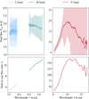 |
Fig. 2 Top row: Measured total flux, Ftot. Bottom row: Derived disk-to-star flux ratio, f°, assuming stellar properties given in Table 2 and wavelength binning as described in Sect. 2. |
Maximum likelihood parameters obtained via a MCMC sampling of the temperature gradient model.
 |
Fig. 3 Best fit of the temperature gradient model with the dust sublimation temperature, Tin, as a free parameter. |
4.3 Discussion
The 2D geometric modeling of a thin disk around a central star results in a best fit, yielding values for the inclination, ι, and position angle, PA, of the inner disk of RY Tau. Compared to the literature values of ιALMA = (65.0 ± 0.1)° and PAALMA = (23.1 ± 01)° of the orientation of the outer disk, the orientation of the inner disk is not (significantly) misaligned, although our fitting method results in a synthetic image of a less inclined (~−5°) and rotated (~−8°) inner disk. GRAVITY Collaboration (2021) reported an inner disk inclination of ιGRAVITY = (60.0 ± 1)° derived from K-band interferometric observations, which is consistent with our analysis of MATISSE observations in the L, M, and N bands. GRAVITY Collaboration (2021) found an inner disk position angle of PAGRAVITY = (8 ± 1)°, which is slightly less (~−5°) than our estimate. In the following analysis, values of ι = 60° and PA = 15° are adopted for self-consistency of the modeling.
The unphysically high dust temperature is an artifact of the simplicity of the chosen model, with Eq. (4) neglecting optical depth effects and backwarming and dust opacities not taken into account. Most importantly, the 2D geometry does not allow for the effect of dust in the LOS to the observer to be modeled, such as diffuse hot circumstellar dust enshrouding the protostar as indicated in previous studies (e.g., Schegerer et al. 2008; Davies et al. 2020) or outflows feeding the disk wind or jet of RY Tau (e.g., Valegård et al. 2022; Takami et al. 2023). Projected onto the image plane, the thermal emission by the enshrouding dust would fill the gap between protostar and disk; as does an unresolved inner rim (which is connected to high dust sublimation temperatures assuming a 2D geometry) employing the temperature gradient model. A 3D radiative transfer model allowing for dust in the LOS to the observer is presented in Sect. 6. Another explanation for an unresolved inner disk rim would be an optically thick gas disk emitting continuum flux, which is explored in Sect. 7.
Finally, the measured closure phases ϕcp ≠ 0 cannot be explained with a model producing a symmetric synthetic flux density map, as the closure phases of such an image are zero. This is the case for the 2D temperature gradient model (see Sect. 4.1). The effect of a flared disk geometry, resulting in an asymmetric brightness distribution, on the closure phases is investigated in Sect. 6.
5 Spatially resolved dust mineralogy
The goal of this section is to analyze the chemical dust composition in the circumstellar environment of RY Tau. The N-band observations shown in Fig. 1 show a strong silicate emission feature in the total flux and correlated fluxes Fcorr at ~10 μm, which is attributed to the Si–O stretching mode (e.g., Henning 2010). The shape of the feature is a superposition of emission features of silicates and other dust materials of different chemical composition (e.g., Bouwman et al. 2001; van Boekel et al. 2004, 2005; Juhász et al. 2010). Additional information contained in the correlated fluxes are the spatial scales in which the emission originates. Following Matter et al. (2020), we estimate the diameter of the spatial region that contributes to a correlated flux spectrum obtained with a projected baseline length Bp and orientation ϕB as ~0.77λ/Bp. Assuming the emission originates from a radially symmetric flat disk with an inclination, ι, and orientation, PA, we define the unresolved disk scale, Δ°, as
![Mathematical equation: $\[\begin{aligned}B_{\mathrm{eff}} & =B_{\mathrm{p}} \sqrt{\cos ^2\left(\phi_{\mathrm{B}}-P A\right)+\cos ^2(\iota) \sin ^2\left(\phi_{\mathrm{B}}-P A\right)}, \\\Delta_{\circ} & \approx 0.77 \frac{\lambda}{B_{\mathrm{eff}}},\end{aligned}\]$](/articles/aa/full_html/2026/01/aa55717-25/aa55717-25-eq15.png) (5)
(5)
via an effective baseline Beff projected onto the disk plane following Varga et al. (2024). The unresolved disk scale can be interpreted as a diameter of a circular region on a flat disk from which the correlated flux of the corresponding baseline originates. The unresolved disk scale per baseline is used as a scale, which is probed by the corresponding correlated flux. The baselines of the observations described in Sect. 2 in the u-v plane and their corresponding unresolved disk scales computed via Eq. (5) for the inclination ι and position angle, PA, determined in Sect. 4 are shown in Fig. 4 for a wavelength of λ = 10 μm.
The correlated fluxes are modeled per baseline j with a similar approach to that in Schegerer et al. (2006), expressed as
![Mathematical equation: $\[F_{\nu; j}=B_\nu\left(T_j\right) \sum_{k=0}^N \mu_{j, k} \varkappa_{\mathrm{abs}; k},\]$](/articles/aa/full_html/2026/01/aa55717-25/aa55717-25-eq16.png) (6)
(6)
where Bν (Tj) is the Planck function for a blackbody with the temperature, Tj, and μj,k are the contributions of each dust component, k, while ϰabs;j,k is the wavelength dependent mass opacity. In this model the parameters Tj and μj,k are fitting parameters and the precomputed unresolved disk scale Δ°(Bp;j) is used to interpret them with respect to spacial region in the disk. The computation of mass opacities for different dust materials is described in Sect. 5.1.
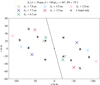 |
Fig. 4 Baselines of the MATISSE observations described in Sect. 2. The dashed line indicates the position angle of the disk major axis in the image plane. |
5.1 Dust opacity model
The opacities of the dust species used in this work are derived from the complex refractive index measurements given in Table 4. The set of silicate materials was selected as by van Boekel et al. (2005) and Schegerer et al. (2006) and was successfully used to fit correlated fluxes of RY Tau by Schegerer et al. (2008). The amorphous silicates (labeled “amorp.” in Table 4) of olivine and pyroxene stoichiometry are referred to as “olivine-type” and “pyroxene-type”, respectively.
The complex refractive index of crystalline materials (labeled “cryst.” in Table 4) is measured with the symmetry axes of the crystal oriented parallel or perpendicular to the electric field vector of the wavefront separately. Depending on crystal symmetry, this results in two or three distinct sets of refractive indices per dust material, which can be combined to model different internal grain structures of dust grains consisting of the same material:
Monocrystalline: Each grain of the dust is assumed to be a monocrystal. The mass opacity of the material is computed from each set of complex refractive indices separately, and the resulting effective medium opacity of the dust is the averaged opacity as the grains are assumed to be arbitrarily oriented with respect to the electromagnetic field vector of the light wave (e.g., Draine 2016).
Polycrystalline: The dust grains are assumed to consist of a composite of multiple crystals of the same material, which are randomly oriented. Therefore, the complex refractive indices measured along different axes are combined into a single set of (n, κ)-values before the mass opacities are derived. To compute effective medium refractive indices, the Bruggeman rule (e.g., Bohren & Huffman 1998) was used in this work.
Different physical processes can induce the crystallization of dust in protoplanetary disks, and the internal dust structure is not known. Furthermore the shape of the dust grains also impacts the resulting opacities (Henning 2010). In this work, we chose to apply the monocrystalline approach to compute opacities for crystalline silicates, and used the polycrystalline approach for graphite. The latter is chosen because graphite contributes to the featureless continuum flux in our model and the optical properties of polycrystalline graphite better resemble a continuum opacity curve in the investigated wavelength range.
In addition to the internal crystal structure, the dust grain shape is relevant for the resulting opacity. In this work, two approaches were employed and compared with respect to their ability to model the observed correlated fluxes of RY Tau:
Classical Mie theory (Mie): Assuming dust as spherical compact grains (Mie 1908).
Distribution of hollow spheres (DHS): Modeling irregular shapes of grains as an effective medium integrated over a distribution of hollow spheres up to a vacuum volume fraction of fmax as proposed by Min et al. (2005).
The opacities are computed using optool (Dominik et al. 2021) for different grain sizes a ∈ {0.1 μm, 1.5 μm, 5 μm}. The resulting mass opacity curves for the selected set of materials, used for the fit of correlated fluxes, are shown in Fig. 5.
Optical properties of materials used in this work.
5.2 Results
The results of the fits on the correlated fluxes for the Mie and DHS opacity models are presented in Figs. A.3 and A.4, respectively. The fit parameters μj,k of the best-fit model are converted to pseudo-mass percentages according to
![Mathematical equation: $\[\mu_{\%; j, k}=\frac{\mu_{j, k}}{\sum_k \mu_{j, k}} \equiv \frac{\mu_{j, k}}{\mu_{\mathrm{tot}; j}},\]$](/articles/aa/full_html/2026/01/aa55717-25/aa55717-25-eq17.png) (7)
(7)
which results in a (mass-)percentage of a certain dust species in the dust mixture. The resulting values are presented in Tables A.1 and A.2. The errors σ%±;j,k are computed from the posterior distribution of probability densities of the parameters assuming a Gaussian distribution. For best-fit parameter values that are low, the estimated posterior distribution differs from a Gaussian profile, as the lower border of the allowed parameter space (μj,k ≥ 0) impacts the distribution. We therefore only consider a dust species detected when the following criteria are both satisfied:
- i)
μ%;j,k − σ%−;j,k ≥ 1 %;
- ii)
μ%;j,k − σ%−;j,k ≥ 0 %.
Criterion i is motivated by a conservative approach to avoid detection of materials with low contributions as their impact on the resulting correlated flux is not relevant with respect to the measurement uncertainty. If criterion i is satisfied, criterion ii considers the posterior probability density distribution, where asymmetry is an indicator for a poorly constrained parameter close to noncontribution. In Tables A.1 and A.2, any nondetection of dust species or grain sizes is marked. The resulting materials in the dust mix differ significantly with respect to the employed grain shape model, described below:
Mie: The silicates detected in the modeled dust mixture are small and medium-sized olivine-type, medium-sized pyroxene-type and medium-sized and large enstatite grains. The continuum contribution is limited to small grains. The ![Mathematical equation: $\[\chi_{\text {red}}^{2}\]$](/articles/aa/full_html/2026/01/aa55717-25/aa55717-25-eq18.png) values are < 0.5 for all baselines, which indicates a good agreement between measured and modeled correlated fluxes. However, a systematic deviation from measured correlated flux shape is observed for unresolved disk scales of Δ° ≤ 6.33 au at λ ~ 11.2 μm.
values are < 0.5 for all baselines, which indicates a good agreement between measured and modeled correlated fluxes. However, a systematic deviation from measured correlated flux shape is observed for unresolved disk scales of Δ° ≤ 6.33 au at λ ~ 11.2 μm.
DHS: All dust species are detected with grains of at least one size contributing to the best fit. Contrary to the Mie model best-fit dust composition, enstatite is less abundant, but small forsterite grains contribute to the correlated fluxes of all baselines. The shape of the modeled correlated fluxes at λ ~ 11.2 μm are closer to the measured shape, which can be attributed to the forsterite contribution. Surprisingly, the ![Mathematical equation: $\[\chi_{\text {red}}^{2}\]$](/articles/aa/full_html/2026/01/aa55717-25/aa55717-25-eq19.png) is higher than in the case of spherical compact grains.
is higher than in the case of spherical compact grains.
To observe trends of crystallinity and grain sizes, the quantities
![Mathematical equation: $\[\begin{aligned}& \mu_{\%; j}(s=\text { const. }) \equiv \frac{\sum_{k \in s=\text { const. }} \mu_{j, k}}{\mu_{\text {tot }; j}}, \text { and } \\& \mu_{\%; j}(a=\text { const. }) \equiv \frac{\sum_{k \in a=\text { const. }} \mu_{j, k}}{\mu_{\text {tot }; j}}\end{aligned}\]$](/articles/aa/full_html/2026/01/aa55717-25/aa55717-25-eq20.png) (8)
(8)
are defined and plotted over the unresolved disk scale Δ° in Figs. A.3 and A.4.
As even those dust species for which no significant abundance was found (i.e., which have not been detected) still contribute to the modeled correlated fluxes and the derived pseudo-masses of grain structure and size, additional MCMC fits for the Mie and DHS grain shape models were performed including only those dust species that were detected. The results are presented in Figs. 6 and 7 and Tables 5 and 6. Although the ![Mathematical equation: $\[\chi_{\text {red}}^{2}\]$](/articles/aa/full_html/2026/01/aa55717-25/aa55717-25-eq21.png) are similarly good for the Mie and DHS grain shape models, the latter approach results in a best fit which matches the „shoulder“ at λ ~ 11.2 μm, most prominently visible in the correlated flux for Δ° = 4.48 au. With respect to internal crystal structure and grain size the following general trends with increasing unresolved disk scale can be observed:
are similarly good for the Mie and DHS grain shape models, the latter approach results in a best fit which matches the „shoulder“ at λ ~ 11.2 μm, most prominently visible in the correlated flux for Δ° = 4.48 au. With respect to internal crystal structure and grain size the following general trends with increasing unresolved disk scale can be observed:
The amount of amorphous dust increases up to an unresolved disk scale of Δ° ≲ 7 au, which is in accordance with the prediction that amorphous grains have undergone annealing, forming crystalline structures at sufficiently high temperatures (e.g., Davoisne et al. 2006).
The contribution of graphite contributing to the featureless flux decreases (up to Δ° ≲ 7 au in the case of the DHS model).
The decrease in small grain sizes is attributed to the decreasing contribution of graphite. For medium-sized and large grains, no unambiguous trends are observed.
These trends are observed for both Mie and DHS models, although the detailed dust species composition differs significantly.
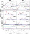 |
Fig. 5 Wavelength-dependent mass absorption opacities derived from complex refractive index measurements for the dust species given in Table 4. Left column: Opacities derived assuming spherical compact grains. Right column: Opacities derived with the DHS approach assuming fmax = 0.7 for the amorphous silicates and graphite and fmax = 0.99 for the crystalline silicates. |
5.3 Discussion
Schegerer et al. (2008) reported an increase in crystallinity and a decrease in the contribution of amorphous dust species with increasing baseline length. In the present work, measurements with six baselines instead of only two have been analyzed, and the trend in crystallinity cannot be confirmed unambiguously. However, a decrease in amorphous silicates close to the central object is found, which suggests that radial mixing, transporting crystalline grains outwards, is taking place. Amorphous silicates close to the inner rim of the disk have undergone annealing, which explains the decrease in their contribution. We extended our dust model by including large grains (a = 5 μm), which appear to be relevant in our fit and are not included in the analysis of the silicate composition done by Schegerer et al. (2008). We also included graphite as representative species for continuum emission and estimated the relative mass of nonsilicate material. A positive trend of continuum emission contribution with decreasing unresolved disk scale is observed.
Surprisingly, using the DHS approach to compute opacities did not result in a better fit than assuming spherical compact grains, although it is expected that the dust in protoplanetary disks is irregularly shaped in reality (e.g., Min et al. 2016). It is, however, noted, that the DHS approach allows us to model correlated flux shapes with a visible “shoulder” at λ = 11.2 μm, which is not possible assuming spherical compact grains. This “shoulder” is related to the tentative detection of forsterite. We conclude that, given the degeneracy of the model and the measurement uncertainties, which are dominated by the large errors of the total flux measurement shown in Fig. 2, we cannot unambiguously determine which grain shape model is better suited to model the measured correlated fluxes.
It is also noted that Eq. (6) is a strong simplification of the temperature structure in an accretion disk, as a single effective temperature Tj per baseline is assumed. A 2D model to investigate the mineralogy of the dust taking into account the spatial structure and temperature gradient of a protoplanetary disk is presented by Varga et al. (2024).
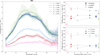 |
Fig. 6 Best-fit model for the dust opacity model assuming spherical compact grains including only detected dust species as given in Table A.1. Left: Comparison of measured and fitted correlated fluxes for the N-band baselines. Upper right: Trends of relative mass contribution of materials depending on their internal structure over unresolved disk scale. Lower right: Trends of grain size over unresolved disk scale. |
 |
Fig. 7 Best-fit model for the dust opacity model assuming a distribution of hollow spheres including only detected dust species as given in Table A.2. Left: Comparison of measured and fitted correlated fluxes for the N-band baselines. Upper right: Trends of relative mass contribution of materials depending on their internal structure over unresolved disk scale. Lower right: Trends of grain size over unresolved disk scale. |
Best fit of relative mass contributions of dust species.
Best fit of relative mass contributions of dust species.
6 Constraining the spatial dust distribution via MCRT simulations
In this section, we present constraints on the 3D dust distribution of the protoplanetary disk of RY Tau. As discussed in Sect. 4.3, the semi-physical 2D modeling approach, assuming a flat disk temperature gradient model, fails to explain the observed closure phases and requires an unphysically high dust temperature to fit the visibilities well. To overcome these issues, we perform MCRT simulations with POLARIS (see Sect. 3) adopting a realistic 3D density distribution, and compute synthetic observations from first principles. The dust distribution of the MCRT model is fitted not only to the measured visibilities, but also to the total flux and closure phases.
6.1 YSO model
The dust density distribution in the inner regions around the protostar of RY Tau is assumed to follow the density distribution of a viscous accretion disk (Shakura & Sunyaev 1973; Lynden-Bell & Pringle 1974). The gas density profile is given by
![Mathematical equation: $\[\begin{aligned}\varrho_{\text {disk}}(r>R_{\text {in}}, z) & =\varrho_{0,\text{disk}}\left(\frac{R_{\text {ref }}}{r}\right)^\alpha \exp \left[-\frac{1}{2}\left(\frac{z}{h(r)}\right)^2\right], \\h(r) & =h_{\text {ref }}\left(\frac{r}{R_{\text {ref }}}\right)^\beta, R_{\text {ref }}=100 ~\mathrm{au},\end{aligned}\]$](/articles/aa/full_html/2026/01/aa55717-25/aa55717-25-eq126.png) (9)
in cylindrical coordinates r, z with the following parameters to be constrained:
(9)
in cylindrical coordinates r, z with the following parameters to be constrained:
The disk density is discretized on a spherical grid with an extent of ![Mathematical equation: $\[R_{\text {max}}=\sqrt{2} R_{\text {out}}=\sqrt{2} \times 35 ~\mathrm{au}\]$](/articles/aa/full_html/2026/01/aa55717-25/aa55717-25-eq127.png) , with Rout chosen sufficiently large to model the circumstellar environment in the field of view of the MATISSE observations (Varga et al. 2024). The reference density ϱ0,disk is related to the total disk mass Mdisk within a cylindrical radius of Rout via
, with Rout chosen sufficiently large to model the circumstellar environment in the field of view of the MATISSE observations (Varga et al. 2024). The reference density ϱ0,disk is related to the total disk mass Mdisk within a cylindrical radius of Rout via
![Mathematical equation: $\[\varrho_{0, \text {disk}}=M_{\text {disk}} \frac{2-\alpha+\beta}{2 \sqrt{2} \pi^{\frac{3}{2}} h_{\text {ref}}\left(R_{\text {out}}^2\left(\frac{R_{\text {ref}}}{R_{\text {out}}}\right)^{\alpha-\beta}-R_{\text {in}}^2\left(\frac{R_{\text {ref}}}{R_{\text {in}}}\right)^{\alpha-\beta}\right)},\]$](/articles/aa/full_html/2026/01/aa55717-25/aa55717-25-eq128.png) (10)
(10)
as given by Burrows et al. (1996). This density distribution of the accretion disk (Eq. (9)) has been successfully used to model the appearance of protoplanetary disks (e.g., Woitke et al. 2016; Robitaille 2017; Woitke et al. 2019).
As a goal of this study is to investigate the influence of diffuse dust elevated above the accretion disk on the appearance of RY Tau in the MIR, a simple-structured envelope is added (e.g., Schegerer et al. 2008). We note that we investigate the dust density distribution of an accretion disk without an envelope in Sect. 6.3. The envelope component accounts for a remnant of the natal envelope or a disk wind enshrouding the protostar. A radial symmetric distribution following
![Mathematical equation: $\[\varrho_{\mathrm{env}}(r>R_{\mathrm{in}})=\varrho_{0, \mathrm{env}}\left(\frac{r}{1 ~\mathrm{au}}\right)^\gamma, \gamma \leq 0\]$](/articles/aa/full_html/2026/01/aa55717-25/aa55717-25-eq129.png) (11)
(11)
is adopted which is combined with the disk density to a model density distribution of
![Mathematical equation: $\[\varrho_{\text {model}}(r>R_{\mathrm{in}}, z)= \begin{cases}\varrho_{\mathrm{disk}}(r, z) & \text { if } \varrho_{\mathrm{disk}}(r, z) \geq \varrho_{\mathrm{env}}(r) \\ \varrho_{\mathrm{env}}(r) & \text { else },\end{cases}\]$](/articles/aa/full_html/2026/01/aa55717-25/aa55717-25-eq130.png) (12)
(12)
with ϱ0,env and γ as additional fitting parameters. We note that we assume a spherical sublimation radius of Rin with a model density of ϱmodel = 0 for r < Rin.
| Rin | inner rim radius; |
| ϱ0,disk | reference density; |
| α | midplane density exponent ϱdisk(r, 0) ∝ r−α; |
| href | reference scale height href ≡ h(Rref); |
| β | flaring exponent. |
6.2 Dust model
The mineralogy of the dust in the circumstellar environment of RY Tau is analyzed in Sec. 5. It is, however, difficult to incorporate the specific results into our radiative transfer simulations for the following reasons:
Incorporating a spatially varying mineralogy into the radiative transfer model would require determining regions in the dust density model in which a certain dust mixture is present. Although the baselines contain information on the spatial region, they also probe a spatial orientation (see Fig. 4) and assume a thin disk emitting at a single temperature. In our 3D density distribution, the temperature is computed self-consistently, resulting in a vertical temperature gradient at a given radial distance from the central object. Keeping in mind that the chemical composition of dust is assumed to be temperature-dependent (e.g., Henning 2010), corresponding radiative transfer models would be required (e.g., Jang et al. 2024).
The complex refractive indices are used to compute the temperature distribution in a protoplanetary disk self-consistently. Therefore, the optical data is not only required in the IR, but also in optical and ultraviolet wavelengths in order to compute passive heating by the central protostar. These data are not available for all considered dust species.
Given the challenges above, we decided to only investigate the density distribution rather than chemical composition of the dust around RY Tau, and adopt a dust model similar to the interstellar medium (ISM) dust composition using astronomical silicate (Draine 2003) as silicate component, which is expected to model the optical properties of dust in protoplanetary disks well in the MIR (Pollack et al. 1994). As in Sect. 5, we use graphite as additional dust component. The mass ratio of astronomical silicate to graphite in the ISM is assumed as ⅝ to ⅜ (Draine 2003). The relative mass ratio for spherical compact graphite grains given in Table A.1 is consistently above a fraction of ⅜ with a ratio of 60% at the shortest unresolved disk scale.
In Sect. 5, single grain sizes are assumed to investigate radial trends in grain size distribution. In our radiative transfer modeling, however, we opt for a continuous grain size distribution according to the Mathis-Rumpl-Nordsieck (MRN; Mathis et al. 1977) distribution with the number density ndust(a) of grain sizes a following the power law dndust(a) ∝ a−3.5 da (Weingartner & Draine 2001). This continuous distribution is commonly adopted for radiative transfer simulations (e.g., Wolf et al. 2003; Schegerer et al. 2008; Sauter et al. 2009; Brunngräber et al. 2016; Hofmann et al. 2022). In order to investigate the effect of grain growth, the maximum grain size amax is varied while the minimum grain size is fixed to amin = 5 nm as suggested by Mathis et al. (1977).
The absorption and scattering properties of the selected dust mixture is computed with the miex algorithm (Wolf & Voshchinnikov 2004), assuming spherical compact grains. As shown in Sect. 5, this simple approach is sufficient to model the observed correlated fluxes in the N band, indicating that choosing a more sophisticated approach is not neccessary. Finally, assuming ideal dust-to-gas coupling, the dust density is set to ϱdust = 0.01 ϱmodel.
6.3 Constraints on the density distribution of the disk
In order to provide constraints on the density distribution of an accretion disk (Eq. (9)) given the dust model described in Sec. 6.2, a set of 1568 parameter combinations was sampled via MCRT simulations. The chosen ranges of the parameter values given in Table 7 cover a broad range of parameters, ensuring that possible best-fit values are included in the covered range. Notably, the reference scale height href and midplane density exponent α values exceed common choices of parameter values used to model protoplanetary disks (e.g., Sauter et al. 2009). We note that the disk mass Mdisk refers to the mass included in a radius of Rout = 35 au, and is therefore not comparable to disk masses derived from observations of the full accretion disk with a radial extent > 70 au (e.g., Long et al. 2019; Francis & van der Marel 2020; Valegård et al. 2022).
To assess the influence of single parameters and their mutual correlations, ![Mathematical equation: $\[\chi_{\text {red}}^{2}\]$](/articles/aa/full_html/2026/01/aa55717-25/aa55717-25-eq131.png) maps are presented for visibilities (Fig. A.5), the total flux (Fig. A.6), and closure phases (Fig.A.7) for a maximum grain size of amax = 250 nm. The lowest
maps are presented for visibilities (Fig. A.5), the total flux (Fig. A.6), and closure phases (Fig.A.7) for a maximum grain size of amax = 250 nm. The lowest ![Mathematical equation: $\[\chi_{\text {red}}^{2}\]$](/articles/aa/full_html/2026/01/aa55717-25/aa55717-25-eq132.png) values for a maximum grain size of amax = 1.5 μm are higher for squared visibilities V2 and total flux Ftot. The maximum grain size has little impact on the general structure of the
values for a maximum grain size of amax = 1.5 μm are higher for squared visibilities V2 and total flux Ftot. The maximum grain size has little impact on the general structure of the ![Mathematical equation: $\[\chi_{\text {red}}^{2}\]$](/articles/aa/full_html/2026/01/aa55717-25/aa55717-25-eq133.png) (V2) distribution in the parameter space. The
(V2) distribution in the parameter space. The ![Mathematical equation: $\[\chi_{\text {red}}^{2}\]$](/articles/aa/full_html/2026/01/aa55717-25/aa55717-25-eq134.png) (Ftot) maps, however, show that the smaller maximum grain size leads to a larger region in the parameter space which yield an acceptable
(Ftot) maps, however, show that the smaller maximum grain size leads to a larger region in the parameter space which yield an acceptable ![Mathematical equation: $\[\chi_{\text {red}}^{2}\]$](/articles/aa/full_html/2026/01/aa55717-25/aa55717-25-eq135.png) . This is consistent with the depletion of large dust grains in the vicinity of the central protostar of RY Tau reported by Francis & van der Marel (2020). In the following we therefore only consider a maximum grain size of amax = 250 nm.
. This is consistent with the depletion of large dust grains in the vicinity of the central protostar of RY Tau reported by Francis & van der Marel (2020). In the following we therefore only consider a maximum grain size of amax = 250 nm.
The degeneracy of the parameter space is well illustrated in Figs. A.5, A.6, and A.7 as there are multiple distinct low ![Mathematical equation: $\[\chi_{\text {red}}^{2}\]$](/articles/aa/full_html/2026/01/aa55717-25/aa55717-25-eq136.png) regions visible for all modeled quantities. Although a good fit (
regions visible for all modeled quantities. Although a good fit (![Mathematical equation: $\[\chi_{\text {red}}^{2}\]$](/articles/aa/full_html/2026/01/aa55717-25/aa55717-25-eq137.png) (V2) = 3.41 and
(V2) = 3.41 and ![Mathematical equation: $\[\chi_{\text {red}}^{2}\]$](/articles/aa/full_html/2026/01/aa55717-25/aa55717-25-eq138.png) (Ftot) = 0.19) is found for the individual observables V2 and Ftot, the regions of low(est)
(Ftot) = 0.19) is found for the individual observables V2 and Ftot, the regions of low(est) ![Mathematical equation: $\[\chi_{\text {red}}^{2}\]$](/articles/aa/full_html/2026/01/aa55717-25/aa55717-25-eq139.png) values in the parameter space are disjoint. Additionally, the closure phases are not reproduced well, and the low
values in the parameter space are disjoint. Additionally, the closure phases are not reproduced well, and the low ![Mathematical equation: $\[\chi_{\text {red}}^{2}\]$](/articles/aa/full_html/2026/01/aa55717-25/aa55717-25-eq140.png) (ϕcp) value regions in the parameter space are disjoint to the other observables.
(ϕcp) value regions in the parameter space are disjoint to the other observables.
The disconnected regions of low ![Mathematical equation: $\[\chi_{\text {red}}^{2}\]$](/articles/aa/full_html/2026/01/aa55717-25/aa55717-25-eq141.png) values in the parameter space for different observables indicate that the model is not sufficiently complex to yield synthetic observations matching the measurements. However, the results of the presented parameter study are highly valuable, as they illustrate the relevant density constraints to model the observations adequately.
values in the parameter space for different observables indicate that the model is not sufficiently complex to yield synthetic observations matching the measurements. However, the results of the presented parameter study are highly valuable, as they illustrate the relevant density constraints to model the observations adequately.
Visibilities: The best fit is achieved for the lowest disk mass of Mdisk = 1 × 10⁻⁷ M⊙, resulting in an optically thin disk. In this regime the modeled closure phases are (almost) zero, as there is little to no asymmetry induced by optical depth effects. MIR observations of highly inclined accretion disks show a shadow cast by the high density region in the disk midplane, which commonly results in an asymmetric flux density distribution. The low ![Mathematical equation: $\[\chi_{\text {red}}^{2}\]$](/articles/aa/full_html/2026/01/aa55717-25/aa55717-25-eq142.png) (V2) value regions for higher disk masses are found for a combination of rather high values of the reference scale height href combined with a low midplane density exponent α, leading to an extended distribution of material, which also results in an optically thin density distribution. The best-fit models for different disk masses share the underestimation of total flux in all bands for Mdisk ≤ 1 × 10⁻⁶ M⊙ and in the L and M bands for Mdisk ≥ 1 × 10⁻⁵ M⊙, while the N-band total flux fits the observation.
(V2) value regions for higher disk masses are found for a combination of rather high values of the reference scale height href combined with a low midplane density exponent α, leading to an extended distribution of material, which also results in an optically thin density distribution. The best-fit models for different disk masses share the underestimation of total flux in all bands for Mdisk ≤ 1 × 10⁻⁶ M⊙ and in the L and M bands for Mdisk ≥ 1 × 10⁻⁵ M⊙, while the N-band total flux fits the observation.
Total flux: The low ![Mathematical equation: $\[\chi_{\text {red}}^{2}\]$](/articles/aa/full_html/2026/01/aa55717-25/aa55717-25-eq143.png) (Ftot) value regions are located at large reference scale heights of href ≥ 25 au, and moderate to high values of the disk midplane density exponent α resulting in a density distribution, which can be heated efficiently. With increasing reference scale height and a fixed disk mass, more dust is distributed in regions with low to medium optical depth above the midplane of the disk, resulting in an increased absorption and thermal reemission efficiency. A higher value of the midplane density exponent increases the amount of dust close to the inner disk rim, where it is heated to higher temperatures compared to regions further away from the central protostar. However, such a density distribution is not in agreement with the observed visibilities.
(Ftot) value regions are located at large reference scale heights of href ≥ 25 au, and moderate to high values of the disk midplane density exponent α resulting in a density distribution, which can be heated efficiently. With increasing reference scale height and a fixed disk mass, more dust is distributed in regions with low to medium optical depth above the midplane of the disk, resulting in an increased absorption and thermal reemission efficiency. A higher value of the midplane density exponent increases the amount of dust close to the inner disk rim, where it is heated to higher temperatures compared to regions further away from the central protostar. However, such a density distribution is not in agreement with the observed visibilities.
Closure phases: More than half of the sampled parameter combinations yield closure phases close to zero. With higher disk masses Mdisk and midplane density exponents α, the midplane gets optically thick and the cast shadow induces an asymmetry, which can explain the observed closure phases which significantly differ from zero.
As indicated by earlier studies (e.g., Schegerer et al. 2008; Takami et al. 2013; Davies et al. 2020), the protostar of RY Tau is enshrouded in dust material, which increases the total flux in the IR if the dust is optically thin. The findings in this section strongly suggest that an optically thin component is necessary to model the observed visibilities. We therefore combine an optically thick accretion disk, which can possibly explain the observed closure phases with an optically thin envelope, as given in Eq. (12).
Parameter combinations used to explore the parameter space of an accretion disk model.
6.4 The influence of a dusty envelope
Adding an envelope to the model (see Eq. (12)) results in two additional fitting parameters, namely the reference density ϱ0;env and density exponent γ of the envelope. A set of simulations to sample the parameter space with the same resolution as in Sec. 6.3 multiplied by the number of different combinations of ϱ0;env and γ would result in a massive computational effort. We therefore opt for a lower resolution parameter sampling to identify regions in the parameter space which are promising with respect to modeling the visibilities, total flux and closure phases. As nonzero closure phases only result from optically thick disks, only high disk masses were taken into account for the combination with an optically thin envelope. The chosen values of γ are motivated by the density power law for an infalling envelope of γ = −0.5 (Ulrich 1976). The coarse resolution parameter space sampling value ranges are given in Table 8 and result in a total of 1536 simulations.
The resulting low(est) ![Mathematical equation: $\[\chi_{\text {red}}^{2}\]$](/articles/aa/full_html/2026/01/aa55717-25/aa55717-25-eq144.png) values do not coincide for the observables V2, Ftot, and ϕcp as for the accretion disk model described in Sect. 6.3. To assess which set of parameters models the observations best, we define the best-fit model as the model which minimizes the sum of
values do not coincide for the observables V2, Ftot, and ϕcp as for the accretion disk model described in Sect. 6.3. To assess which set of parameters models the observations best, we define the best-fit model as the model which minimizes the sum of ![Mathematical equation: $\[\chi_{\text {red}}^{2}\]$](/articles/aa/full_html/2026/01/aa55717-25/aa55717-25-eq145.png) (V2) and
(V2) and ![Mathematical equation: $\[\chi_{\text {red}}^{2}\]$](/articles/aa/full_html/2026/01/aa55717-25/aa55717-25-eq146.png) (Ftot). As the
(Ftot). As the ![Mathematical equation: $\[\chi_{\text {red}}^{2}\]$](/articles/aa/full_html/2026/01/aa55717-25/aa55717-25-eq147.png) (ϕcp) values are much higher than the
(ϕcp) values are much higher than the ![Mathematical equation: $\[\chi_{\text {red}}^{2}\]$](/articles/aa/full_html/2026/01/aa55717-25/aa55717-25-eq148.png) values of the other two observables, it is unfeasible to take them into account as they would dominate the criterion. The results for the best-fit model with an accretion disk and envelope are presented in Fig. 8. The parameters of the best-fit model are given in Table 9.
values of the other two observables, it is unfeasible to take them into account as they would dominate the criterion. The results for the best-fit model with an accretion disk and envelope are presented in Fig. 8. The parameters of the best-fit model are given in Table 9.
As the closure phases in Fig. 8 indicate that the best-fit model lacks some asymmetry, an additional set of simulations was run with a refined resolution of sampled parameter values in the region of the parameter space, where shading of the outer disk regions from starlight by a dense inner disk midplane results in an asymmetric synthetic flux density map. This is achieved with disk masses Mdisk ≥ 1 × 10⁻⁵ M⊙, reference scale heights href < 25 au and a large midplane density exponent α ≥ 1.8. In order to reduce the number of free parameters, which allows us to choose a higher resolution for the remaining free parameters, the envelope density exponent was fixed to the theoretical value γ = −0.5, as the coarse parameter space sampling showed that its influence on the resulting synthetic observables is small compared to the influence of the reference density of the envelope ϱ0,env. Additionally, the range of parameter values of the latter is reduced to the relevant region in the parameter space. The resolution and range of free parameter values used to explore the parameter space in combination with a dense midplane of the disk is given in Table 10. The resulting best fit with respect to visibilities and total flux is shown in Fig. 9. The corresponding ![Mathematical equation: $\[\chi_{\text {red}}^{2}\]$](/articles/aa/full_html/2026/01/aa55717-25/aa55717-25-eq149.png) maps for a disk mass of Mdisk = 1 × 10⁻⁴ M⊙ on visibilities, total flux and closure phases are shown in Figs. A.8, A.9, and A.10, respectively. The disk mass Mdisk has little impact on the position of the low
maps for a disk mass of Mdisk = 1 × 10⁻⁴ M⊙ on visibilities, total flux and closure phases are shown in Figs. A.8, A.9, and A.10, respectively. The disk mass Mdisk has little impact on the position of the low ![Mathematical equation: $\[\chi_{\text {red}}^{2}\]$](/articles/aa/full_html/2026/01/aa55717-25/aa55717-25-eq150.png) (V2) region in the parameter space, while shifting the regions of low
(V2) region in the parameter space, while shifting the regions of low ![Mathematical equation: $\[\chi_{\text {red}}^{2}\]$](/articles/aa/full_html/2026/01/aa55717-25/aa55717-25-eq151.png) (Ftot) toward higher reference scale heights of the disk, which leads to disjoint regions of low
(Ftot) toward higher reference scale heights of the disk, which leads to disjoint regions of low ![Mathematical equation: $\[\chi_{\text {red}}^{2}\]$](/articles/aa/full_html/2026/01/aa55717-25/aa55717-25-eq152.png) on visibilities and total flux. The structure of the four-dimensional parameter space for Mdisk = 1 × 10⁻⁴ M⊙ shows that the quality of the fit only weakly depends on the midplane density exponent α within the chosen parameter range. Consequently, the parameters Mdisk and α are not well constrained if the midplane of the innermost disk is optically thick (i.e., Mdisk > 1 × 10⁻⁵ M⊙, α ≥ 1.8 and href < 30 au). Additionally, a strong correlation between reference scale height href and reference density of the envelope ϱ0,env with respect to the resulting
on visibilities and total flux. The structure of the four-dimensional parameter space for Mdisk = 1 × 10⁻⁴ M⊙ shows that the quality of the fit only weakly depends on the midplane density exponent α within the chosen parameter range. Consequently, the parameters Mdisk and α are not well constrained if the midplane of the innermost disk is optically thick (i.e., Mdisk > 1 × 10⁻⁵ M⊙, α ≥ 1.8 and href < 30 au). Additionally, a strong correlation between reference scale height href and reference density of the envelope ϱ0,env with respect to the resulting ![Mathematical equation: $\[\chi_{\text {red}}^{2}\]$](/articles/aa/full_html/2026/01/aa55717-25/aa55717-25-eq153.png) on the visibilities is revealed in the
on the visibilities is revealed in the ![Mathematical equation: $\[\chi_{\text {red}}^{2}\]$](/articles/aa/full_html/2026/01/aa55717-25/aa55717-25-eq154.png) maps. This further illustrates the degeneracy of the parameter space. The regions with low
maps. This further illustrates the degeneracy of the parameter space. The regions with low ![Mathematical equation: $\[\chi_{\text {red}}^{2}\]$](/articles/aa/full_html/2026/01/aa55717-25/aa55717-25-eq155.png) values for visibilities and total flux, although generally disjoint, slightly overlap for small disk reference scale heights and a flaring parameter of β = 1.1, where the best-fit parameters of the model shown in Fig. 9 are located in the parameter space (see Figs. A.8 and A.9). Compared to the best fit found in the coarse parameter study with an envelope, the best-fit criterion
values for visibilities and total flux, although generally disjoint, slightly overlap for small disk reference scale heights and a flaring parameter of β = 1.1, where the best-fit parameters of the model shown in Fig. 9 are located in the parameter space (see Figs. A.8 and A.9). Compared to the best fit found in the coarse parameter study with an envelope, the best-fit criterion ![Mathematical equation: $\[\min \left(\chi_{\text {red}}^{2}\left(V^{2}\right)+\chi_{\text {red}}^{2}\left(F_{\text {tot}}\right)\right)\]$](/articles/aa/full_html/2026/01/aa55717-25/aa55717-25-eq156.png) is higher, which can be mainly attributed to the total flux, which is overestimated in the N band. However, the synthetic closure phases at long baselines in the L and M bands fit the observations well. In the N band, the synthetic closure phases are significantly larger than for the model shown in Fig. 8, but the model shown in Fig. 9 fails to fully reproduce the observed asymmetry. We note that the modeled N-band closure phases for the shorter two triplets with shortest maximum baseline lengths Bp;max fit the observations poorly, which explains the larger value of
is higher, which can be mainly attributed to the total flux, which is overestimated in the N band. However, the synthetic closure phases at long baselines in the L and M bands fit the observations well. In the N band, the synthetic closure phases are significantly larger than for the model shown in Fig. 8, but the model shown in Fig. 9 fails to fully reproduce the observed asymmetry. We note that the modeled N-band closure phases for the shorter two triplets with shortest maximum baseline lengths Bp;max fit the observations poorly, which explains the larger value of ![Mathematical equation: $\[\chi_{\text {red}}^{2}\]$](/articles/aa/full_html/2026/01/aa55717-25/aa55717-25-eq157.png) (ϕcp) compared to the “disk only” and “disk and envelope” model (see Table 9).
(ϕcp) compared to the “disk only” and “disk and envelope” model (see Table 9).
Conclusively, we found two different parameter combinations for the accretion disk and envelope model, which fit the observed visibilities similarly well:
Lower mass, strongly flared disk: Best fit with respect to the numerical value of the best-fit criterion including visibilities and total flux. However, the modeled closure phases are close to zero, which contradicts the observations.
Higher mass, thin disk: The observed closure phases can be modeled to some extent, maintaining a good fit on the visibilities at the cost of total flux overestimation in the N band. The minimum value of the best-fit criterion is slightly smaller than for the best-fit disk model without an envelope shown in Fig. A.2.
The corresponding model density and temperature distributions are shown in Figs. A.11 and A.12, respectively. The density distributions show that hot dust is present in the LOS to the central protostar of RY Tau, confirming the results by Davies et al. (2020). The observed closure phases suggest that this dust is part of an envelope or disk wind, and not of the upper disk layers. We conclude that an optically thin envelope in combination with an accretion disk is the best model to produce synthetic observations that fit the MIR appearance of the inner disk of RY Tau, confirming the results by Schegerer et al. (2008). We finally note that an envelope model without a disk employing the density distribution given in Eq. (11) is able to model the total flux well, while it fails to explain the observed visibilities and closure phases in a reasonable value range of ϱ0,env ∈ [1 × 10⁻¹⁵ kg m−3, 1 × 10⁻¹² kg m−3] and γ ∈ [−1.2, −0.3].
An open question remaining is the origin of the discrepancy between the observed and modeled N band closure phases. Possible explanations include an induced shadow by infalling material as proposed by Krieger et al. (2024) or an intrinsic asymmetric density distribution in the disk (e.g., Varga et al. 2021; Juhász et al. 2025). Moreover, our modeling suggests that the asymmetry in the flux density in the L band can be explained by an accretion disk combined with an envelope, while the asymmetry in the N band is of a different origin and not visible in the L band. As longer wavelengths allow us to probe regions closer to the disk midplane, an embedded accreting companion visible in the N band, but obscured by the upper disk layers in the L band, represents another possible origin of the observed closure phases.
Parameter combinations on a coarse grid used to explore the parameter space of an accretion disk combined with a dusty envelope.
 |
Fig. 8 Best-fit model of the accretion disk model with an optically thin envelope. The model parameters are listed in Table 9. The pink ellipses in the intensity maps indicate the half-light radii of the emitting region measured in the disk midplane as defined by Varga et al. (2018). |
Best-fit values for the different parameter spaces sampled via MCRT simulations.
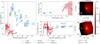 |
Fig. 9 Best-fit model of an accretion disk with a dense midplane and an additional optically thin envelope. The model parameters are listed in Table 9. |
Parameter combinations on a refined grid used to explore the parameter space of a dense midplane accretion disk combined with a dusty envelope.
6.5 Apparent size of RY Tau
Using the best-fit disk and envelope model as basis for the size estimation in the L, M, and N bands, the half-light radius rhl(λ) as defined in Varga et al. (2018) was computed numerically on the intensity maps at wavelengths of 3.58 μm, 4.78 μm, and 10.6 μm, respectively. The resulting L-band and M-band half-light radii are rhl(3.58 μm) = ![Mathematical equation: $\[3.5_{-0.5}^{+0.5}\]$](/articles/aa/full_html/2026/01/aa55717-25/aa55717-25-eq162.png) mas and rhl(4.58 μm) =
mas and rhl(4.58 μm) = ![Mathematical equation: $\[4.9_{-0.5}^{+0.5}\]$](/articles/aa/full_html/2026/01/aa55717-25/aa55717-25-eq163.png) mas. For comparison, the K-band half-light radius found by GRAVITY Collaboration (2021) is
mas. For comparison, the K-band half-light radius found by GRAVITY Collaboration (2021) is ![Mathematical equation: $\[2.45_{-0.22}^{+0.24}\]$](/articles/aa/full_html/2026/01/aa55717-25/aa55717-25-eq164.png) mas.
mas.
In the N band, our radiative transfer model results in a significantly larger value of rhl(10.6 μm) = ![Mathematical equation: $\[33.6_{-0.5}^{+0.5}\]$](/articles/aa/full_html/2026/01/aa55717-25/aa55717-25-eq165.png) mas compared to the estimate of
mas compared to the estimate of ![Mathematical equation: $\[8.0_{-0.7}^{+0.7}\]$](/articles/aa/full_html/2026/01/aa55717-25/aa55717-25-eq166.png) mas found by Varga et al. (2018). Considering the rather high χ2 of the best-fit model found by Varga et al. (2018) used to compute the half-light radius, our estimate is better constrained by the MATISSE observations. The ellipses in the image plane, corresponding to rhl(λ) from within Ftot(λ)/2 is emitted, are shown in Fig. 8.
mas found by Varga et al. (2018). Considering the rather high χ2 of the best-fit model found by Varga et al. (2018) used to compute the half-light radius, our estimate is better constrained by the MATISSE observations. The ellipses in the image plane, corresponding to rhl(λ) from within Ftot(λ)/2 is emitted, are shown in Fig. 8.
6.6 Photometry from the optical to MIR
As a consistency check of the best-fit models of an accretion disk and envelope given in Table 9, the total flux measurements in L, M, and N bands shown in Fig. 2 are supplemented with photometry in the optical and NIR (SDSS, Pan-STARRS, 2MASS Ahn et al. 2012; Chambers et al. 2016; Skrutskie et al. 2006) and the Spitzer spectrum (Lebouteiller et al. 2011; Espaillat et al. 2011) observed with the Infrared Spectrograph (IRS; Houck et al. 2004) instrument in the MIR to compare the synthetic SED produced by our models to observations in a broad wavelength range. The photometry and synthetic SEDs for the lower mass and strongly flared disk (Mdisk = 1 × 10⁻⁵ M⊙) and the higher mass and thin and dense midplane disk (Mdisk = 1 × 10⁻⁴ M⊙) are shown in Fig. 10. As expected, the photometry is highly variable in the optical, indicating that both models represent an active state of RY Tau. Comparing the MATISSE total flux measurements to the Spitzer spectrum, no evidence for MIR variability is found. The model with the lower disk mass overestimates the total flux at short wavelengths, while the higher mass model fits the photometry in the optical well. In the NIR, both models underestimate the total flux. Toward longer wavelengths in the MIR beyond the N band, the higher mass disk model overestimates the total flux. As we expect that larger grains settled to the midplane of the accretion disk, which are not included in our modeling, would contribute to the total flux in this wavelength range, the overestimation indicates that a disk mass of Mdisk = 1 × 10⁻⁴ M⊙ is too high. As the total disk mass is poorly constrained if the disk midplane is optically thick, the flux overestimation toward longer wavelengths in the MIR of the “dense disk and envelope” (see Table 9) model does not rule out the possibility of RY Tau hosting a dense midplane and geometrically thin accretion disk. A possibility to explain the mismatch between our models and the 2MASS photometry in the NIR is the accretion luminosity, which is reported to be relevant to model the appearance of RY Tau by Akeson et al. (2005) and Schegerer et al. (2008).
We also note that the shape of the SED with respect to the broad wavelength range shown in Fig. 10 depends on the dust composition. While we only used polycrystalline graphite as continuum emitting material, iron and organic materials are expected to exist in protoplanetary disks (e.g., Birnstiel et al. 2018; Varga et al. 2024), possibly impacting the broad range shape of the SED. Additionally, the internal structure of graphite itself, while irrelevant in the L, M and N bands, has an impact on the resulting SED toward longer wavelengths.
7 The impact of accretion
To estimate the impact of accretion luminosity on the observables in the L, M and N bands, we employ a simple accretion model similar to the one implemented by Schegerer et al. (2008). To justify the negligence of accretion effects in the modeling presented in Sect. 6, we calculate the total flux released in the accretion process and assess its contribution to the observed SED. The mass accretion rate ![Mathematical equation: $\[\dot{M}\]$](/articles/aa/full_html/2026/01/aa55717-25/aa55717-25-eq167.png) of RY Tau is reported to be 3.6 × 10⁻⁸ M⊙ yr−1 by Petrov et al. (2019) and 2.7 × 10⁻⁸ M⊙ yr−1 by Alcalá et al. (2021) which are both in the error interval of the value range 6.4 × 10⁻⁸−9.1 × 10⁻⁸ M⊙ yr−1 given in an earlier study by Petrov et al. (1999). We therefore assumed a value of 3 × 10⁻⁸ M⊙ yr−1 to estimate the flux contribution by the energy release in the accretion process. To this means, we used the best-fit accretion disk and envelope model with a disk mass of Mdisk = 1 × 10⁻⁵ M⊙ (Fig. 8) and included the accretion luminosity into the model to assess its influence on the resulting SED. Following, e.g., Pringle (1981), the accretion luminosity is given by
of RY Tau is reported to be 3.6 × 10⁻⁸ M⊙ yr−1 by Petrov et al. (2019) and 2.7 × 10⁻⁸ M⊙ yr−1 by Alcalá et al. (2021) which are both in the error interval of the value range 6.4 × 10⁻⁸−9.1 × 10⁻⁸ M⊙ yr−1 given in an earlier study by Petrov et al. (1999). We therefore assumed a value of 3 × 10⁻⁸ M⊙ yr−1 to estimate the flux contribution by the energy release in the accretion process. To this means, we used the best-fit accretion disk and envelope model with a disk mass of Mdisk = 1 × 10⁻⁵ M⊙ (Fig. 8) and included the accretion luminosity into the model to assess its influence on the resulting SED. Following, e.g., Pringle (1981), the accretion luminosity is given by
![Mathematical equation: $\[\begin{gathered}L_{\mathrm{acc}}(R_{\star} \leq r<\infty)=\int_{R_{\star}}^{\infty} D_{\mathrm{acc}}(r) 2 \pi r ~d r=\frac{G \dot{M} M_{\star}}{2 R_{\star}}, \\D_{\mathrm{acc}}(r)=\frac{3 G M_{\star} \dot{M}}{4 \pi r^3}\left(1-\sqrt{\frac{R_{\star}}{r}}\right).\end{gathered}\]$](/articles/aa/full_html/2026/01/aa55717-25/aa55717-25-eq168.png) (13)
(13)
The total gravitational potential loss of accreting material is
![Mathematical equation: $\[E_{\mathrm{grav}}=\frac{G M \dot{M}}{R_{\star}}=2 L_{\mathrm{acc}}(R_{\star} \leq r<\infty),\]$](/articles/aa/full_html/2026/01/aa55717-25/aa55717-25-eq169.png) (14)
(14)
with Egrav/2 converted to kinetic energy, which is realeased in a boundary layer above the stellar photosphere (Pringle 1981). As Schegerer et al. (2008), we take accretion effects in different parts of our YSO model into account:
- i)
R⋆ ≤ r < Rbnd: The infalling gas interacts with the magnetic field forming strong shocks (Calvet & Gullbring 1998). The shock layers above the stellar photosphere are assumed to emit blackbody radiation at a temperature of Tbnd = 8000 K (Muzerolle et al. 2003). Assuming magnetic field strengths ~kG, we adopted a value for the magnetic boundary radius of Rbnd = 5 R⋆ as Akeson et al. (2005). To test if this region has a significant impact on the observed SED in the NIR and MIR, we performed a MCRT simulation of the best-fit model including an additional energy release of Lacc(R⋆ ≤ r < Rbnd) + Egrav/2 = 0.17 L⊙ + 0.29 L⊙ from the stellar photosphere assuming an accretion rate of
![Mathematical equation: $\[\dot{M}\]$](/articles/aa/full_html/2026/01/aa55717-25/aa55717-25-eq170.png) = 3 × 10⁻⁸ M⊙ yr−1. The simulation showed that this has a negligible impact on the SED from the optical to the MIR. We note that the impact of accretion needs to be considered if the accretion rate is in the range of the upper limit of the error interval given by Petrov et al. (1999), which is
= 3 × 10⁻⁸ M⊙ yr−1. The simulation showed that this has a negligible impact on the SED from the optical to the MIR. We note that the impact of accretion needs to be considered if the accretion rate is in the range of the upper limit of the error interval given by Petrov et al. (1999), which is ![Mathematical equation: $\[\dot{M}\]$](/articles/aa/full_html/2026/01/aa55717-25/aa55717-25-eq171.png) = 1.4 × 10⁻⁷ M⊙ yr−1.
= 1.4 × 10⁻⁷ M⊙ yr−1.
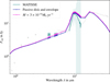
Fig. 11 Contribution of accretion luminosity to the modeled SED considering i) emission by shock-heated gas accreting onto the stellar photosphere and ii) an optically thick gas disk between the magnetic boundary radius of the central protostar and the dust sublimation rim of the accretion disk.
- ii)
Rbnd ≤ r < Rin: The accretion luminosity is modeled as an infinitely thin, optically thick gas disk emitting as a blackbody with the radial temperature given by Pringle (1981)
![Mathematical equation: $\[T_{\mathrm{gas}}(r)=\left(\frac{3 G M_{\star} \dot{M}}{8 \pi R^3 \sigma_{\mathrm{SB}}}\left(1-\sqrt{\frac{R_{\star}}{r}}\right)\right)^{\frac{1}{4}}.\]$](/articles/aa/full_html/2026/01/aa55717-25/aa55717-25-eq172.png) (15)
(15)A similar approach has been implemented by Akeson et al. (2005). The flux arriving at the detector is computed by
![Mathematical equation: $\[F_{\mathrm{acc}}=\frac{1}{d^2} \int_{R_{\mathrm{bnd}}}^{R_{\mathrm{in}}} B_v(T_{\mathrm{gas}}) ~d r,\]$](/articles/aa/full_html/2026/01/aa55717-25/aa55717-25-eq173.png) (16)
(16)resulting in an additional total flux in the NIR, as shown in Fig. 11.
We note that the accretion flux originating from this region is added to the detector without taking into account the interaction with the dust in the circumstellar environment. As the dust of the best-fit YSO model in the LOS from observer to the direct stellar vicinity is optically thin, the attenuation of Facc is neglected in order to estimate the upper limit of the impact of accretion luminosity on the NIR and MIR photometry.
- iii)
Rin ≤ r: As the dissipation rate Dacc(r) of infalling material given in Eq. (13) drops rapidly with increasing radial distance from the central star r, the energy release in this region can be neglected (Akeson et al. 2005; Schegerer et al. 2008).
The SED taking the energy release in the accretion process in regions i) and ii) into account is compared to the SED of the best-fit model of a passively heated disk with an envelope in Fig. 11. We conclude that the impact of accretion can be neglected for the modeling of RY Tau observations in the L, M and N bands, as it has very little impact on the SED, and consequently on the visibilities. We note that the unrealistic scenario of a higher accretion rate and a smaller magnetic boundary radius would increase the NIR and MIR flux significantly.
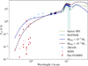 |
Fig. 10 Comparison of the synthetic SED produced by the MCRT best-fits models presented in Sect. 6.4 with photometry measurements. The models are distinguished by their disk mass Mdisk and the remaining parameters of the accretion disk and envelope model are given in Table 9. |
8 Conclusions
We present the first MATISSE observations in the L, M, and N bands of the inner disk of the YSO RY Tau. The data were analyzed with respect to mineralogy and spatial distribution of the dust in the immediate vicinity of the central protostar of the accretion disk.
We estimated the accretion disk orientation fitting a 2D temperature gradient disk model to the observed visibilities, resulting in an inclination of ι = 60° and position angle of PA = 15°, which suggests no significant misalignment of inner and outer disk. However, the model suggests an unresolved inner rim of the accretion disk, which would result in unphysically high dust sublimation temperatures. Employing 3D radiative transfer models, we demonstrated that hot dust in the LOS to the protostar of RY Tau resolves this issue;
The dust composition was analyzed by applying a simple single-temperature model. Various silicate species, commonly found in protoplanetary disk, have been detected. Within the measurement accuracy and degeneracy of the modeling results, we cannot determine the dust grain shape, and found similar good fits on the N-band correlated fluxes with spherical compact grain and DHS models. We report a strong dependence on the continuum, crystalline, and amorphous contribution, as well as that of grain size on baseline length and orientation. We found an increase in the graphite abundance, representing the contribution of featureless flux, along with a decrease in the amount of amorphous silicate grains with decreasing unresolved disk scale, with the latter attributed to annealing;
The spatial distribution of dust around the protostar of RY Tau has been constrained with MCRT simulations. We confirmed earlier results by Schegerer et al. (2008), that an accretion disk with an envelope fits the observations best. On the basis of our best-fit model, we estimate the half-light radii of the emitting region measured in the disk midplane as rhl,L = 0.5 au, rhl,M = 0.7 au, and rhl,N = 4.7 au in the L, M, and N bands, respectively. Based on recent accretion rate results by Petrov et al. (2019) and Alcalá et al. (2021), we find that accretion luminosity is negligible in the MIR. Our systematic exploration of the multidimensional parameter space revealed a strong degeneracy. We demonstrate that a strongly flared and thick disk, as well as a flat and dense disk, with scale heights of h(5 au) = 0.61 au and h(5 au) = 0.28 au, respectively, in combination with an envelope fit the observed visibilities well. The latter is in agreement with the results by Davies et al. (2020) analyzing interferometric observations of RY Tau in the K band. This model also explains the observed closure phases in the L band, but overestimates the total flux toward longer wavelengths. However, the specific origin of the observed asymmetry, appearing only in the N band, cannot be further constrained on the basis of our observations.
Our analysis suggests that moderately inclined transition disks, such as the protoplanetary disk of RY Tau, cannot be necessarily modeled well assuming a flat disk. Taking into account the effect of hot dust in the LOS to the observer, possibly making up part of a disk wind, is required to interpret the MATISSE observations of RY Tau. The use of radiative transfer models, taking into account 3D effects of the dust distribution, scattering, and accretion luminosity, would plausibly be required to interpret similar observations of other protoplanetary disks. In the case of RY Tau, closure phases in the L and M band up to ±5° can be explained by a flared disk geometry, without requiring any disk substructure.
Acknowledgements
MATISSE was designed, funded and built in close collaboration with ESO, by a consortium composed of institutes in France (J.-L. Lagrange Laboratory – INSU-CNRS – Côte d’Azur Observatory – University of Côte d’Azur), Germany (MPIA, MPIfR and University of Kiel), The Netherlands (NOVA and University of Leiden), and Austria (University of Vienna). The Konkoly Observatory and Cologne University have also provided some support in the manufacture of the instrument. This research was supported in part through high-performance computing resources available at the Kiel University Computing Centre. JV is funded from the Hungarian NKFIH OTKA projects no. K-132406, and K-147380. This work was also supported by the NKFIH NKKP grant ADVANCED 149943 and the NKFIH excellence grant TKP2021-NKTA-64. Project no.149943 has been implemented with the support provided by the Ministry of Culture and Innovation of Hungary from the National Research, Development and Innovation Fund, financed under the NKKP ADVANCED funding scheme. JV acknowledges support from the Fizeau exchange visitors programme. The research leading to these results has received funding from the European Union’s Horizon 2020 research and innovation programme under Grant Agreement 101004719 (ORP). LL gratefully acknowledges the Collaborative Research Center 1601 funded by the Deutsche Forschungsgemeinschaft (DFG, German Research Foundation)—SFB 1601 [sub-project A3]—500700252. This research has made use of the services of the ESO Science Archive Facility. This research has made use of the OIFITS 2 data exchange standard for optical interferometry (Duvert et al. 2017) using the Python module oifits publicly available via https://github.com/pboley/oifits. This research has made use of the VizieR catalogue access tool, CDS, Strasbourg, France (DOI: 10.26093/cds/vizier). The original description of the VizieR service was published in Ochsenbein et al. (2000). Funding for SDSS-III has been provided by the Alfred P. Sloan Foundation, the Participating Institutions, the National Science Foundation, and the U.S. Department of Energy Office of Science. The SDSS-III web site is http://www.sdss3.org/. SDSS-III is managed by the Astrophysical Research Consortium for the Participating Institutions of the SDSS-III Collaboration including the University of Arizona, the Brazilian Participation Group, Brookhaven National Laboratory, Carnegie Mellon University, University of Florida, the French Participation Group, the German Participation Group, Harvard University, the Instituto de Astrofisica de Canarias, the Michigan State/Notre Dame/JINA Participation Group, Johns Hopkins University, Lawrence Berkeley National Laboratory, Max Planck Institute for Astrophysics, Max Planck Institute for Extraterrestrial Physics, New Mexico State University, New York University, Ohio State University, Pennsylvania State University, University of Portsmouth, Princeton University, the Spanish Participation Group, University of Tokyo, University of Utah, Vanderbilt University, University of Virginia, University of Washington, and Yale University.
References
- Ahn, C. P., Alexandroff, R., Allende Prieto, C., et al. 2012, ApJS, 203, 21 [Google Scholar]
- Akaike, H. 1974, IEEE Trans. Automatic Control, 19, 716 [CrossRef] [Google Scholar]
- Akeson, R. L., Walker, C. H., Wood, K., et al. 2005, ApJ, 622, 440 [Google Scholar]
- Alcalá, J. M., Gangi, M., Biazzo, K., et al. 2021, A&A, 652, A72 [NASA ADS] [CrossRef] [EDP Sciences] [Google Scholar]
- Alexander, R. D., Clarke, C. J., & Pringle, J. E. 2006, MNRAS, 369, 229 [CrossRef] [Google Scholar]
- Andrews, S. M., Wilner, D. J., Espaillat, C., et al. 2011, ApJ, 732, 42 [Google Scholar]
- Babina, E. V., Artemenko, S. A., & Petrov, P. P. 2016, Astron. Lett., 42, 193 [NASA ADS] [CrossRef] [Google Scholar]
- Bailer-Jones, C. A. L., Rybizki, J., Fouesneau, M., Demleitner, M., & Andrae, R. 2021, AJ, 161, 147 [Google Scholar]
- Bensberg, A., & Wolf, S. 2022, A&A, 668, A120 [NASA ADS] [CrossRef] [EDP Sciences] [Google Scholar]
- Birnstiel, T., Dullemond, C. P., Zhu, Z., et al. 2018, ApJ, 869, L45 [CrossRef] [Google Scholar]
- Bjorkman, J. E., & Wood, K. 2001, ApJ, 554, 615 [NASA ADS] [CrossRef] [Google Scholar]
- Bohn, A. J., Benisty, M., Perraut, K., et al. 2022, A&A, 658, A183 [NASA ADS] [CrossRef] [EDP Sciences] [Google Scholar]
- Bohren, C. F., & Huffman, D. R. 1998, Absorption and Scattering of Light by Small Particles (Wiley-VCH) [Google Scholar]
- Bouwman, J., Meeus, G., de Koter, A., et al. 2001, A&A, 375, 950 [NASA ADS] [CrossRef] [EDP Sciences] [Google Scholar]
- Brown, J. M., Blake, G. A., Dullemond, C. P., et al. 2007, ApJ, 664, L107 [Google Scholar]
- Brunngräber, R., Wolf, S., Ratzka, T., & Ober, F. 2016, A&A, 585, A100 [NASA ADS] [CrossRef] [EDP Sciences] [Google Scholar]
- Burrows, C. J., Stapelfeldt, K. R., Watson, A. M., et al. 1996, ApJ, 473, 437 [Google Scholar]
- Calvet, N., & Gullbring, E. 1998, ApJ, 509, 802 [Google Scholar]
- Calvet, N., D’Alessio, P., Hartmann, L., et al. 2002, ApJ, 568, 1008 [Google Scholar]
- Calvet, N., Muzerolle, J., Briceño, C., et al. 2004, AJ, 128, 1294 [NASA ADS] [CrossRef] [Google Scholar]
- Cardelli, J. A., Clayton, G. C., & Mathis, J. S. 1989, ApJ, 345, 245 [Google Scholar]
- Chambers, K. C., Magnier, E. A., Metcalfe, N., et al. 2016, arXiv e-prints [arXiv:1612.05560], accessed via VizieR On-line Data Catalog: II/349. [Google Scholar]
- Davies, C. L., Kraus, S., Harries, T. J., et al. 2020, ApJ, 897, 31 [NASA ADS] [CrossRef] [Google Scholar]
- Davoisne, C., Djouadi, Z., Leroux, H., et al. 2006, A&A, 448, L1 [NASA ADS] [CrossRef] [EDP Sciences] [Google Scholar]
- Dominik, C., Min, M., & Tazaki, R. 2021, OpTool: Command-line driven tool for creating complex dust opacities, Astrophysics Source Code Library [record ascl:2104.010] [Google Scholar]
- Dorschner, J., Begemann, B., Henning, T., Jäger, C., & Mutschke, H. 1995, A&A, 300, 503 [NASA ADS] [Google Scholar]
- Draine, B. T. 2003, ApJ, 598, 1026 [Google Scholar]
- Draine, B. T. 2016, ApJ, 831, 109 [NASA ADS] [CrossRef] [Google Scholar]
- Dullemond, C. P., & Dominik, C. 2005, A&A, 434, 971 [CrossRef] [EDP Sciences] [Google Scholar]
- Dullemond, C. P., & Monnier, J. D. 2010, ARA&A, 48, 205 [Google Scholar]
- Duschl, W. J., Gail, H. P., & Tscharnuter, W. M. 1996, A&A, 312, 624 [NASA ADS] [Google Scholar]
- Duvert, G., Young, J., & Hummel, C. A. 2017, A&A, 597, A8 [NASA ADS] [CrossRef] [EDP Sciences] [Google Scholar]
- Espaillat, C., Furlan, E., D’Alessio, P., et al. 2011, ApJ, 728, 49 [NASA ADS] [CrossRef] [Google Scholar]
- Foreman-Mackey, D., Hogg, D. W., Lang, D., & Goodman, J. 2013, PASP, 125, 306 [Google Scholar]
- Francis, L., & van der Marel, N. 2020, ApJ, 892, 111 [Google Scholar]
- Gaia Collaboration (Vallenari, A., et al.) 2023, A&A, 674, A1 [NASA ADS] [CrossRef] [EDP Sciences] [Google Scholar]
- Galli, P. A. B., Loinard, L., Ortiz-Léon, G. N., et al. 2018, ApJ, 859, 33 [Google Scholar]
- Garufi, A., Benisty, M., Pinilla, P., et al. 2018, A&A, 620, A94 [NASA ADS] [CrossRef] [EDP Sciences] [Google Scholar]
- Garufi, A., Podio, L., Bacciotti, F., et al. 2019, A&A, 628, A68 [NASA ADS] [CrossRef] [EDP Sciences] [Google Scholar]
- Garufi, A., Ginski, C., van Holstein, R. G., et al. 2024, A&A, 685, A53 [NASA ADS] [CrossRef] [EDP Sciences] [Google Scholar]
- Goodman, J., & Weare, J. 2010, Commun. Appl. Math. Computat. Sci., 5, 65 [Google Scholar]
- GRAVITY Collaboration (Perraut, K., et al.) 2021, A&A, 655, A73 [NASA ADS] [CrossRef] [EDP Sciences] [Google Scholar]
- Harrison, R. E., Lin, Z.-Y. D., Looney, L. W., et al. 2024, ApJ, 967, 40 [Google Scholar]
- Henning, T. 2010, ARA&A, 48, 21 [Google Scholar]
- Hofmann, K. H., Bensberg, A., Schertl, D., et al. 2022, A&A, 658, A81 [NASA ADS] [CrossRef] [EDP Sciences] [Google Scholar]
- Hogg, D. W., Bovy, J., & Lang, D. 2010, arXiv e-prints [arXiv:1008.4686] [Google Scholar]
- Houck, J. R., Roellig, T. L., van Cleve, J., et al. 2004, ApJS, 154, 18 [NASA ADS] [CrossRef] [Google Scholar]
- Isella, A., Carpenter, J. M., & Sargent, A. I. 2010, ApJ, 714, 1746 [Google Scholar]
- Jäger, C., Mutschke, H., Begemann, B., Dorschner, J., & Henning, T. 1994, A&A, 292, 641 [NASA ADS] [Google Scholar]
- Jäger, C., Molster, F. J., Dorschner, J., et al. 1998, A&A, 339, 904 [NASA ADS] [Google Scholar]
- Jang, H., Waters, R., Kamp, I., & Dullemond, C. P. 2024, A&A, 687, A275 [NASA ADS] [CrossRef] [EDP Sciences] [Google Scholar]
- Juhász, A., Bouwman, J., Henning, T., et al. 2010, ApJ, 721, 431 [Google Scholar]
- Juhász, T., Varga, J., Ábrahám, P., et al. 2025, ApJ, 982, 36 [Google Scholar]
- Kenyon, S. J., Dobrzycka, D., & Hartmann, L. 1994, AJ, 108, 1872 [NASA ADS] [CrossRef] [Google Scholar]
- Keppler, M., Benisty, M., Müller, A., et al. 2018, A&A, 617, A44 [NASA ADS] [CrossRef] [EDP Sciences] [Google Scholar]
- Kley, W., & Nelson, R. P. 2012, ARA&A, 50, 211 [Google Scholar]
- Kobus, J., Wolf, S., Ratzka, T., & Brunngräber, R. 2020, A&A, 642, A104 [NASA ADS] [CrossRef] [EDP Sciences] [Google Scholar]
- Krieger, A., Kuffmeier, M., Reissl, S., et al. 2024, A&A, 686, A111 [NASA ADS] [CrossRef] [EDP Sciences] [Google Scholar]
- Lada, C. J. 1987, in IAU Symposium, 115, Star Forming Regions, eds. M. Peimbert, & J. Jugaku, 1 [Google Scholar]
- Lazareff, B., Berger, J. P., Kluska, J., et al. 2017, A&A, 599, A85 [NASA ADS] [CrossRef] [EDP Sciences] [Google Scholar]
- Lebouteiller, V., Barry, D. J., Spoon, H. W. W., et al. 2011, ApJS, 196, 8 [NASA ADS] [CrossRef] [Google Scholar]
- Leinert, C., Graser, U., Przygodda, F., et al. 2003, Ap&SS, 286, 73 [Google Scholar]
- Lin, D. N. C., & Papaloizou, J. 1979, MNRAS, 188, 191 [Google Scholar]
- Long, F., Herczeg, G. J., Harsono, D., et al. 2019, ApJ, 882, 49 [Google Scholar]
- Lopez, B., Lagarde, S., Petrov, R. G., et al. 2022, A&A, 659, A192 [NASA ADS] [CrossRef] [EDP Sciences] [Google Scholar]
- Lynden-Bell, D., & Pringle, J. E. 1974, MNRAS, 168, 603 [Google Scholar]
- Mathis, J. S., Rumpl, W., & Nordsieck, K. H. 1977, ApJ, 217, 425 [Google Scholar]
- Matter, A., Pignatale, F. C., & Lopez, B. 2020, MNRAS, 497, 2540 [NASA ADS] [CrossRef] [Google Scholar]
- Mattila, K. 1970, A&A, 9, 53 [NASA ADS] [Google Scholar]
- Menu, J., van Boekel, R., Henning, T., et al. 2015, A&A, 581, A107 [NASA ADS] [CrossRef] [EDP Sciences] [Google Scholar]
- Meskini, C., Sauty, C., Marcowith, A., Vlahakis, N., & Brunn, V. 2024, A&A, 686, A287 [NASA ADS] [CrossRef] [EDP Sciences] [Google Scholar]
- Mie, G. 1908, Ann. Phys., 330, 377 [Google Scholar]
- Millour, F., Berio, P., Heininger, M., et al. 2016, SPIE Conf. Ser., 9907, 990723 [NASA ADS] [Google Scholar]
- Min, M., Hovenier, J. W., & de Koter, A. 2005, A&A, 432, 909 [NASA ADS] [CrossRef] [EDP Sciences] [Google Scholar]
- Min, M., Rab, C., Woitke, P., Dominik, C., & Ménard, F. 2016, A&A, 585, A13 [NASA ADS] [CrossRef] [EDP Sciences] [Google Scholar]
- Monnier, J. D., Berger, J. P., Millan-Gabet, R., et al. 2006, ApJ, 647, 444 [NASA ADS] [CrossRef] [Google Scholar]
- Muzerolle, J., Calvet, N., Hartmann, L., & D’Alessio, P. 2003, ApJ, 597, L149 [NASA ADS] [CrossRef] [Google Scholar]
- Nakajima, T., & Golimowski, D. A. 1995, AJ, 109, 1181 [NASA ADS] [CrossRef] [Google Scholar]
- Ochsenbein, F., Bauer, P., & Marcout, J. 2000, A&AS, 143, 23 [NASA ADS] [CrossRef] [EDP Sciences] [Google Scholar]
- Penzlin, A. B. T., Booth, R. A., Nelson, R. P., Schäfer, C. M., & Kley, W. 2024, MNRAS, 532, 3166 [Google Scholar]
- Petrov, P. P., Zajtseva, G. V., Efimov, Y. S., et al. 1999, A&A, 341, 553 [NASA ADS] [Google Scholar]
- Petrov, P. P., Grankin, K. N., Gameiro, J. F., et al. 2019, MNRAS, 483, 132 [NASA ADS] [CrossRef] [Google Scholar]
- Petrov, P. P., Romanova, M. M., Grankin, K. N., et al. 2021, MNRAS, 504, 871 [NASA ADS] [CrossRef] [Google Scholar]
- Pollack, J. B., Hollenbach, D., Beckwith, S., et al. 1994, ApJ, 421, 615 [Google Scholar]
- Pringle, J. E. 1981, ARA&A, 19, 137 [Google Scholar]
- Regály, Z., Juhász, A., Sándor, Z., & Dullemond, C. P. 2012, MNRAS, 419, 1701 [Google Scholar]
- Reissl, S., Wolf, S., & Brauer, R. 2016, A&A, 593, A87 [NASA ADS] [CrossRef] [EDP Sciences] [Google Scholar]
- Reissl, S., Wolf, S., & Brauer, R. 2018, POLARIS: POLArized RadIation Simulator, Astrophysics Source Code Library, [record ascl:1807.001] [Google Scholar]
- Ribas, Á., Espaillat, C. C., Macías, E., et al. 2017, ApJ, 849, 63 [NASA ADS] [CrossRef] [Google Scholar]
- Robitaille, T. P. 2017, A&A, 600, A11 [NASA ADS] [CrossRef] [EDP Sciences] [Google Scholar]
- Sauter, J., Wolf, S., Launhardt, R., et al. 2009, A&A, 505, 1167 [NASA ADS] [CrossRef] [EDP Sciences] [Google Scholar]
- Sauty, C., de Albuquerque, R. M. G., Cayatte, V., Lima, J. J. G., & Gameiro, J. F. 2022, A&A, 664, A176 [NASA ADS] [CrossRef] [EDP Sciences] [Google Scholar]
- Schegerer, A., Wolf, S., Voshchinnikov, N. V., Przygodda, F., & Kessler-Silacci, J. E. 2006, A&A, 456, 535 [NASA ADS] [CrossRef] [EDP Sciences] [Google Scholar]
- Schegerer, A. A., Wolf, S., Ratzka, T., & Leinert, C. 2008, A&A, 478, 779 [NASA ADS] [CrossRef] [EDP Sciences] [Google Scholar]
- Shakura, N. I., & Sunyaev, R. A. 1973, A&A, 24, 337 [NASA ADS] [Google Scholar]
- Skinner, S. L., Audard, M., & Güdel, M. 2016, ApJ, 826, 84 [Google Scholar]
- Skinner, S. L., Schneider, P. C., Audard, M., & Güdel, M. 2018, ApJ, 855, 143 [NASA ADS] [CrossRef] [Google Scholar]
- Skrutskie, M. F., Cutri, R. M., Stiening, R., et al. 2006, AJ, 131, 1163 [NASA ADS] [CrossRef] [Google Scholar]
- Smith, N., Bally, J., Licht, D., & Walawender, J. 2005, AJ, 129, 382 [NASA ADS] [CrossRef] [Google Scholar]
- St-Onge, G., & Bastien, P. 2008, ApJ, 674, 1032 [NASA ADS] [CrossRef] [Google Scholar]
- Takami, M., Karr, J. L., Hashimoto, J., et al. 2013, ApJ, 772, 145 [Google Scholar]
- Takami, M., Günther, H. M., Schneider, P. C., et al. 2023, ApJS, 264, 1 [NASA ADS] [CrossRef] [Google Scholar]
- Tazzari, M., Beaujean, F., & Testi, L. 2018, MNRAS, 476, 4527 [Google Scholar]
- Ulrich, R. K. 1976, ApJ, 210, 377 [Google Scholar]
- Vaidya, B., Fendt, C., & Beuther, H. 2009, ApJ, 702, 567 [NASA ADS] [CrossRef] [Google Scholar]
- Valegård, P. G., Waters, L. B. F. M., & Dominik, C. 2021, A&A, 652, A133 [NASA ADS] [CrossRef] [EDP Sciences] [Google Scholar]
- Valegård, P. G., Ginski, C., Dominik, C., et al. 2022, A&A, 668, A25 [NASA ADS] [CrossRef] [EDP Sciences] [Google Scholar]
- van Boekel, R., Min, M., Leinert, C., et al. 2004, Nature, 432, 479 [NASA ADS] [CrossRef] [Google Scholar]
- van Boekel, R., Min, M., Waters, L. B. F. M., et al. 2005, A&A, 437, 189 [NASA ADS] [CrossRef] [EDP Sciences] [Google Scholar]
- Varga, J., Ábrahám, P., Chen, L., et al. 2018, A&A, 617, A83 [NASA ADS] [CrossRef] [EDP Sciences] [Google Scholar]
- Varga, J., Gabányi, K. É., Ábrahám, P., et al. 2017, A&A, 604, A84 [NASA ADS] [CrossRef] [EDP Sciences] [Google Scholar]
- Varga, J., Hogerheijde, M., van Boekel, R., et al. 2021, A&A, 647, A56 [NASA ADS] [CrossRef] [EDP Sciences] [Google Scholar]
- Varga, J., Waters, L. B. F. M., Hogerheijde, M., et al. 2024, A&A, 681, A47 [NASA ADS] [CrossRef] [EDP Sciences] [Google Scholar]
- Villenave, M., Stapelfeldt, K. R., Duchêne, G., et al. 2024, ApJ, 961, 95 [NASA ADS] [CrossRef] [Google Scholar]
- Weigelt, G., Grinin, V. P., Groh, J. H., et al. 2011, A&A, 527, A103 [NASA ADS] [CrossRef] [EDP Sciences] [Google Scholar]
- Weingartner, J. C., & Draine, B. T. 2001, ApJ, 548, 296 [Google Scholar]
- Williams, J. P., & Cieza, L. A. 2011, ARA&A, 49, 67 [Google Scholar]
- Woitke, P., Min, M., Pinte, C., et al. 2016, A&A, 586, A103 [NASA ADS] [CrossRef] [EDP Sciences] [Google Scholar]
- Woitke, P., Kamp, I., Antonellini, S., et al. 2019, PASP, 131, 064301 [NASA ADS] [CrossRef] [Google Scholar]
- Wolf, S., & Voshchinnikov, N. V. 2004, Comput. Phys. Commun., 162, 113 [Google Scholar]
- Wolf, S., Henning, T., & Stecklum, B. 1999, A&A, 349, 839 [NASA ADS] [Google Scholar]
- Wolf, S., Padgett, D. L., & Stapelfeldt, K. R. 2003, ApJ, 588, 373 [NASA ADS] [CrossRef] [Google Scholar]
- Yusef-Zadeh, F., Morris, M., & White, R. L. 1984, ApJ, 278, 186 [CrossRef] [Google Scholar]
- Zeidler, S., Posch, T., & Mutschke, H. 2013, A&A, 553, A81 [NASA ADS] [CrossRef] [EDP Sciences] [Google Scholar]
- Zeidler, S., Mutschke, H., & Posch, T. 2015, ApJ, 798, 125 [Google Scholar]
The true distance to RY Tau is currently unknown and different values are used in recent literature. While Harrison et al. (2024) used a value of d = 128 pc, VizieR (Ochsenbein et al. 2000) lists a value of d = 161 pc derived from Gaia Collaboration (2023) parallax measurements. As the distance impacts the luminosity estimation, we chose to follow the approach by Davies et al. (2020) selecting a consistent set of stellar parameters. The adopted distance is very close to the value of d = 139 pc estimated by Bailer-Jones et al. (2021).
Appendix A Additional material
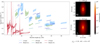 |
Fig. A.1 Best fit of the temperature gradient model with a fixed dust sublimation temperature of Tin = 1500 K. |
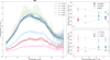 |
Fig. A.3 Best-fit model for the dust opacity model assuming spherical compact grains. Left: Comparison of measured and fitted correlated fluxes for the N-band baselines. Upper right: Trends of relative mass contribution of materials depending on their internal structure over unresolved disk scale. Lower right: Trends of grain size over unresolved disk scale. |
Best fit of relative mass contributions of dust species in the compositional analysis fit on correlated fluxes in the N band assuming spherical compact grains. Any nondetection of a certain dust species is indicated by gray values.
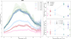 |
Fig. A.4 Best-fit model for the dust opacity model assuming a distribution of hollow spheres. Left: Comparison of measured and fitted correlated fluxes for the N-band baselines. Upper right: Trends of relative mass contribution of materials depending on their internal structure over unresolved disk scale. Lower right: Trends of grain size over unresolved disk scale. |
Best fit of relative mass contributions of dust species in the compositional analysis fit on correlated fluxes in the N band employing the DHS opacity model. Any nondetection of a certain dust species is indicated by gray values.
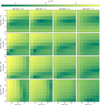 |
Fig. A.5
|
![Mathematical equation: $\[\chi_{\text {red}}^{2}\]$](/articles/aa/full_html/2026/01/aa55717-25/aa55717-25-eq392.png)
![Mathematical equation: $\[\chi_{\text {red}}^{2}\]$](/articles/aa/full_html/2026/01/aa55717-25/aa55717-25-eq393.png)
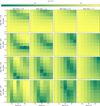 |
Fig. A.6
|
![Mathematical equation: $\[\chi_{\text {red}}^{2}\]$](/articles/aa/full_html/2026/01/aa55717-25/aa55717-25-eq394.png)
![Mathematical equation: $\[\chi_{\text {red}}^{2}\]$](/articles/aa/full_html/2026/01/aa55717-25/aa55717-25-eq395.png)
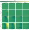 |
Fig. A.7
|
![Mathematical equation: $\[\chi_{\text {red}}^{2}\]$](/articles/aa/full_html/2026/01/aa55717-25/aa55717-25-eq396.png)
![Mathematical equation: $\[\chi_{\text {red}}^{2}\]$](/articles/aa/full_html/2026/01/aa55717-25/aa55717-25-eq397.png)
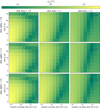 |
Fig. A.8
|
![Mathematical equation: $\[\chi_{\text {red}}^{2}\]$](/articles/aa/full_html/2026/01/aa55717-25/aa55717-25-eq398.png)
![Mathematical equation: $\[\chi_{\text {red}}^{2}\]$](/articles/aa/full_html/2026/01/aa55717-25/aa55717-25-eq399.png)
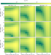 |
Fig. A.9
|
![Mathematical equation: $\[\chi_{\text {red}}^{2}\]$](/articles/aa/full_html/2026/01/aa55717-25/aa55717-25-eq400.png)
![Mathematical equation: $\[\chi_{\text {red}}^{2}\]$](/articles/aa/full_html/2026/01/aa55717-25/aa55717-25-eq401.png)
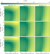 |
Fig. A.10
|
![Mathematical equation: $\[\chi_{\text {red}}^{2}\]$](/articles/aa/full_html/2026/01/aa55717-25/aa55717-25-eq402.png)
![Mathematical equation: $\[\chi_{\text {red}}^{2}\]$](/articles/aa/full_html/2026/01/aa55717-25/aa55717-25-eq403.png)
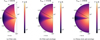 |
Fig. A.12 Temperature distributions computed by MCRT simulations for the model density distributions shown in Fig. A.11 of the MCRT models listed in Table 9. We note that the radius r is scaled logarithmically. |
All Tables
Maximum likelihood parameters obtained via a MCMC sampling of the temperature gradient model.
Parameter combinations used to explore the parameter space of an accretion disk model.
Parameter combinations on a coarse grid used to explore the parameter space of an accretion disk combined with a dusty envelope.
Parameter combinations on a refined grid used to explore the parameter space of a dense midplane accretion disk combined with a dusty envelope.
Best fit of relative mass contributions of dust species in the compositional analysis fit on correlated fluxes in the N band assuming spherical compact grains. Any nondetection of a certain dust species is indicated by gray values.
Best fit of relative mass contributions of dust species in the compositional analysis fit on correlated fluxes in the N band employing the DHS opacity model. Any nondetection of a certain dust species is indicated by gray values.
All Figures
|
Fig. 1 Overview of the MATISSE observations of RY Tau listed in Table 1. The corresponding u–v coordinates are shown in Fig. 4. Left panel: Squared visibilities, V2, over projected baseline length Bp (pink/red: 8–13 μm wavelengths; blue/green: 3.5–5.2 μm wavelengths; see color bars). Middle panel: Measured closure phases, ϕcp, over the longest projected baseline length in the telescope triplet, Bp;max. Right panel: Correlated fluxes, Fcorr, and corresponding projected baseline length, Bp, and orientation, ϕB, in the N band. |
| In the text | |
|
Fig. 2 Top row: Measured total flux, Ftot. Bottom row: Derived disk-to-star flux ratio, f°, assuming stellar properties given in Table 2 and wavelength binning as described in Sect. 2. |
| In the text | |
|
Fig. 3 Best fit of the temperature gradient model with the dust sublimation temperature, Tin, as a free parameter. |
| In the text | |
|
Fig. 4 Baselines of the MATISSE observations described in Sect. 2. The dashed line indicates the position angle of the disk major axis in the image plane. |
| In the text | |
|
Fig. 5 Wavelength-dependent mass absorption opacities derived from complex refractive index measurements for the dust species given in Table 4. Left column: Opacities derived assuming spherical compact grains. Right column: Opacities derived with the DHS approach assuming fmax = 0.7 for the amorphous silicates and graphite and fmax = 0.99 for the crystalline silicates. |
| In the text | |
|
Fig. 6 Best-fit model for the dust opacity model assuming spherical compact grains including only detected dust species as given in Table A.1. Left: Comparison of measured and fitted correlated fluxes for the N-band baselines. Upper right: Trends of relative mass contribution of materials depending on their internal structure over unresolved disk scale. Lower right: Trends of grain size over unresolved disk scale. |
| In the text | |
|
Fig. 7 Best-fit model for the dust opacity model assuming a distribution of hollow spheres including only detected dust species as given in Table A.2. Left: Comparison of measured and fitted correlated fluxes for the N-band baselines. Upper right: Trends of relative mass contribution of materials depending on their internal structure over unresolved disk scale. Lower right: Trends of grain size over unresolved disk scale. |
| In the text | |
|
Fig. 8 Best-fit model of the accretion disk model with an optically thin envelope. The model parameters are listed in Table 9. The pink ellipses in the intensity maps indicate the half-light radii of the emitting region measured in the disk midplane as defined by Varga et al. (2018). |
| In the text | |
|
Fig. 9 Best-fit model of an accretion disk with a dense midplane and an additional optically thin envelope. The model parameters are listed in Table 9. |
| In the text | |
|
Fig. 10 Comparison of the synthetic SED produced by the MCRT best-fits models presented in Sect. 6.4 with photometry measurements. The models are distinguished by their disk mass Mdisk and the remaining parameters of the accretion disk and envelope model are given in Table 9. |
| In the text | |
|
Fig. 11 Contribution of accretion luminosity to the modeled SED considering i) emission by shock-heated gas accreting onto the stellar photosphere and ii) an optically thick gas disk between the magnetic boundary radius of the central protostar and the dust sublimation rim of the accretion disk. |
| In the text | |
|
Fig. A.1 Best fit of the temperature gradient model with a fixed dust sublimation temperature of Tin = 1500 K. |
| In the text | |
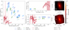 |
Fig. A.2 Best-fit model of the accretion disk model. The model parameters are listed in Table 9. |
| In the text | |
|
Fig. A.3 Best-fit model for the dust opacity model assuming spherical compact grains. Left: Comparison of measured and fitted correlated fluxes for the N-band baselines. Upper right: Trends of relative mass contribution of materials depending on their internal structure over unresolved disk scale. Lower right: Trends of grain size over unresolved disk scale. |
| In the text | |
|
Fig. A.4 Best-fit model for the dust opacity model assuming a distribution of hollow spheres. Left: Comparison of measured and fitted correlated fluxes for the N-band baselines. Upper right: Trends of relative mass contribution of materials depending on their internal structure over unresolved disk scale. Lower right: Trends of grain size over unresolved disk scale. |
| In the text | |
|
Fig. A.5
|
| In the text | |
|
Fig. A.6
|
| In the text | |
|
Fig. A.7
|
| In the text | |
|
Fig. A.8
|
| In the text | |
|
Fig. A.9
|
| In the text | |
|
Fig. A.10
|
| In the text | |
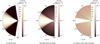 |
Fig. A.11 Density distributions of the MCRT models listed in Table 9. |
| In the text | |
|
Fig. A.12 Temperature distributions computed by MCRT simulations for the model density distributions shown in Fig. A.11 of the MCRT models listed in Table 9. We note that the radius r is scaled logarithmically. |
| In the text | |
Current usage metrics show cumulative count of Article Views (full-text article views including HTML views, PDF and ePub downloads, according to the available data) and Abstracts Views on Vision4Press platform.
Data correspond to usage on the plateform after 2015. The current usage metrics is available 48-96 hours after online publication and is updated daily on week days.
Initial download of the metrics may take a while.