© The Authors 2025

1. Introduction

The geometry and structure of cosmic fields evolve from initial homogeneity due to expansion and gravitational forces (Bardeen et al. 1986; Bernardeau et al. 2002). These fields reflect the expansion history of the Universe and the growth of substructures. Although small-scale structures are influenced by gravitational and baryonic interactions, large-scale structures result primarily from gravitational instabilities, forming the so-called cosmic web made of voids, walls, filaments, and halos (Bond et al. 1996).

Traditionally, these structures are studied using correlation functions or power spectra (e.g. Peebles & Groth 1975; Fry 1985), which provide limited insights into the intricate web-like patterns. Alternative approaches focus on topology and geometry, employing tools such as Minkowski functionals, Betti numbers, and persistent homology (e.g. White 1979; Matsubara 1994; Mecke et al. 1994; Gay et al. 2012; Press & Schechter 1974; Pranav et al. 2017). Critical points in the density field, where gradients vanish, serve as useful statistical probes and are increasingly studied for cosmological insights, including clustering analyses (e.g. Bardeen et al. 1986; Cadiou et al. 2020).

A related yet significant concept is Rayleigh-Lévy flights (Klages et al. 2008), which describe scale-independent non-Gaussian processes and are useful in modelling the motion of dark halos. They differ from standard Markovian processes by exhibiting long-range correlations and hierarchical properties, making them a simplified yet statistically insightful representation of the fully non-linear cosmic density field. They were first introduced in astrophysics by Holtsmark (1919) to capture fluctuations in gravitational systems (see Litovchenko 2021, for more recent work). Lévy flights are simply defined as a Markov chain point process whose jump probability depends on some power law of the length of the jump alone (Mandelbrot 1975; Peebles 1980; Szapudi & Colombi 1996; Uchaikin 2019). As such, they capture anomalous diffusion and are related to first-passage theory (Krapivsky et al. 2010) and Press-Schechter halo formation (Press & Schechter 1974).

Previous work Bernardeau (2022), Bernardeau & Pichon (2024) derived from first principle one- and two-point statistics for the critical points of smoothed sampled realisation of these Rayleigh-Lévy flights in one to three dimensions. They provided closed-form expressions for Euler counts and their clustering correlations in the mean-field limit, describing their long-separation behaviour. They also presented quadratures for calculating critical point number densities. Their result was validated by Monte Carlo simulations in one dimension only. Following Bernardeau & Pichon (2024), the present study focuses on validating in two dimensions using the Minkowski functionals – a set of summary statistics comprising the probability density function (PDF) of the density field, the total perimeter length of iso-field contours, and the Euler characteristic, which together characterise the non-Gaussianity of the field’s one-point distribution. We restrict ourselves to expansion beyond the mean field (MF) for the density PDF and iso-field perimeter, W₁, and leave the exploration of quantities such as Euler characteristics or extrema counts in 2D to future work.

The rest of this work proceeds as follows. Section 2 recalls the main relevant properties of Rayleigh-Lévy flights. Section 3 discusses beyond-mean-field corrections in two dimensions. Comparisons to Monte-Carlo simulations are provided throughout for validation in Sect. 4. Section 5 presents our conclusions. Appendix A shows the cumulant generating functions (CGFs) beyond the MF and the corresponding skewness, converging to the exact value. Appendix B presents a general derivation of the PDF of the iso-field perimeter. Appendix C presents tests that were performed to ensure the robustness of the simulations.

2. Rayleigh Lévy flight model

We first briefly review the basic properties of Rayleigh-Lévy flights and the MF limit, discussed in detail in Bernardeau (2022), Bernardeau & Pichon (2024).

2.1. Basics

A Rayleigh-Lévy flight is a point distribution for which each successive point is a step from the previous, in a random direction and with a length drawn from a cumulative probability distribution function of the form

$$\begin{array}{c}\hfill \mathrm{CDF}(l)=\{\begin{array}{cc}0\hfill & ,l<l_0\hfill \\ 1-{(l_0/l)}^{\alpha }\hfill & ,l\ge l_0.\hfill \end{array}\end{array}$$(1)

The resulting flights are characterised by rare long jumps, independent of the box size. These are usually handled using periodic boundary conditions. Figure 1 illustrates a Rayleigh-Lévy flight with periodic boundary conditions in two dimensions.

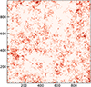Fig. 1. Two-dimensional Rayleigh-Lévy flight with parameters α = 3/2 and ξ0 ∼ 2.47 (ℓ0 = 0.01), a density of Npts = 40 points per pixel, a box width of L = 4000 × Δ, a resolution of Δ = 0.25, and a Gaussian smoothing scale of R = 1.

In D dimensions, the two-point correlation functions for flights between positions r₁ and r₂ is given by

$$\begin{array}{c}\hfill \xi ({\mathbf{r}}_1,{\mathbf{r}}_2)=\frac{1}{n}{\displaystyle \int \frac{d^D\mathbf{k}}{{(2\pi )}^D}}{e}^{i\mathbf{k}·({\mathbf{r}}_2-{\mathbf{r}}_1)}\frac{2}{1-\psi (k)},\end{array}$$(2)

where n is the number density of points and ψ(k) is the Fourier transform of f₁(r), the density of the subsequent point at position r (first descendant of a given point at position r₀). For a Rayleigh-Lévy flight, this is given by

$$\begin{array}{c}\hfill f_1(\mathbf{r})=\frac{\alpha \mathrm{\Gamma }(D/2+1)}{2{\pi }^{D/2}}\frac{{\ell }_0^{\alpha }}{|\mathbf{r}-{\mathbf{r}}_0{|}^{D+\alpha }}\end{array}$$(3)

for |r−r₀| > 1₀. The large distance correlation (kl₀ ≪ 1 or 1 − ψ(k)∼(ℓ₀k)^α) behaves like

$$\begin{array}{c}\hfill \xi ({\mathbf{r}}_1,{\mathbf{r}}_2)\sim r^{\alpha -D}{\ell }_0^{-\alpha }/n.\end{array}$$(4)

This is subject to constraints α < D and 0 < α < 2; the first is required to avoid a logarithmic divergence at k = 0 and the second comes from the expected behavior of ψ(k) at low k, $\psi (k)=1-{(l_{0}k)}^{\alpha }+\mathcal{O}(k^2)$¹.

The statistical properties of the field can be inferred through its CGF. In principle, having the CGF is tantamount to having the cumulants of the density, its gradient, and the corresponding probability distribution function (PDF), i.e.

$$\begin{array}{c}\hfill \phi ({\lambda }_1,\dots ,{\lambda }_n)={\displaystyle \sum _{p_1,\dots ,p_n}}{⟨{\rho }_1^{p_1}\dots {\rho }_n^{p_n}⟩}_c\frac{{\lambda }_1^{p_1}}{p_1!}.\end{array}$$(5)

In particular, the one-point skewness, 𝒮₃, of the density, ρ, can be derived by expanding the CGF in power of λ ≡ λ_ρ up to the third order,

$$\begin{array}{c}\hfill \phi (\lambda )=\lambda +{\xi }_0\frac{{\lambda }^2}{2!}+{\mathcal{S}}_3\frac{{\xi }_0^2{\lambda }^3}{3!}+\mathcal{O}\left({\lambda }^4\right).\end{array}$$(6)

The PDF of the density can be computed as

$$\begin{array}{cc}\hfill P(\rho )& ={\displaystyle {\int }_{-i\infty }^{+i\infty }}\frac{d\lambda }{2\pi i}exp(-\lambda \rho +\phi (\lambda ))\hfill \\ \hfill & ={\displaystyle {\int }_{-i\infty }^{+i\infty }}\frac{d\lambda }{2\pi i}\frac{e^{-\lambda \rho +\phi (\lambda )}{\partial }_{\lambda }\phi (\lambda )}{\rho }-\frac{e^{-\lambda \rho +\phi (\lambda )}}{2\pi i\rho }{|}_{-i\infty }^{i\infty }.\hfill \end{array}$$

The second line is easier to deal with in practice.

The remaining piece required to estimate the PDF of the density field is a recipe for the CGF. This is provided by the hierarchical tree model (Appendix B of Bernardeau & Pichon 2024). In this case, the CGF can be approximated via the set of equations

$$\begin{array}{cc}\hfill \phi ({\lambda }_1,\dots ,{\lambda }_n)& ={\displaystyle \sum _j}{\lambda }_j{\displaystyle \int {\mathrm{d}}^2\mathbf{x}}{\mathcal{C}}_j(\mathbf{x})(1+\tau (\mathbf{x})/2)\hfill \end{array}$$(7)

and

$$\begin{array}{c}\hfill \tau (\mathbf{x})={\displaystyle \sum _j}{\lambda }_j{\displaystyle \int {\mathrm{d}}^2{\mathbf{x}}^{\prime }}{\mathcal{C}}_j({\mathbf{x}}^{\prime })\xi (\mathbf{x},{\mathbf{x}}^{\prime })(1+\tau ({\mathbf{x}}^{\prime })/2),\end{array}$$(8)

where φ(λ₁, …, λ_n) is the CGF, τ(x) is the rooted-CGF (r-CGF), 𝒞_j(x) is a window function in the jth cell, and ξ(x,x′) is the two-point correlation function². This is used in the next section to study the properties of Rayleigh-Lévy flights in the so-called MF limit.

2.2. Mean field

In the MF approximation, the r-CGF is assumed to be constant within each cell. This is reasonable for compact, non-compensated, spherically symmetric density profiles. Denoting with τ_i the value of the r-CGF for each cell, i, we averaged Eq. (8) over the cell, i, with profile 𝒞_i(x) to obtain

$$\begin{array}{c}\hfill {\tau }_i={\displaystyle \sum _j}{\lambda }_j(1+{\tau }_j/2){\displaystyle \int d\mathbf{x}}{\displaystyle \int d{\mathbf{x}}^{\prime }}{\mathcal{C}}_i(\mathbf{x}){\mathcal{C}}_j({\mathbf{x}}^{\prime })\xi (\mathbf{x},{\mathbf{x}}^{\prime }).\end{array}$$(9)

Then, for the one-point CGF, Eq. (9) gives the implicit equation

$$\begin{array}{c}\hfill {\tau }_1={\lambda }_1{\xi }_0(1-{\tau }_1/2),\end{array}$$(10)

where ξ₀ is the average two-point correlation function in a cell,

$$\begin{array}{c}\hfill {\xi }_0={\displaystyle \int d\mathbf{x}d{\mathbf{x}}^{\prime }}{\mathcal{C}}_1(\mathbf{x}){\mathcal{C}}_1({\mathbf{x}}^{\prime })\xi (\mathbf{x},{\mathbf{x}}^{\prime }).\end{array}$$(11)

The CGF of a Rayleigh-Lévy flight in the MF limit is therefore

$$\begin{array}{c}\hfill {\phi }_1({\lambda }_{\rho };{\xi }_0)=\frac{2{\lambda }_{\rho }}{2-{\xi }_0{\lambda }_{\rho }}·\end{array}$$(12)

Take note that this can be expanded as

$$\begin{array}{c}\hfill \phi ({\lambda }_{\rho })={\lambda }_{\rho }+{\xi }_0\frac{{\lambda }_{\rho }^2}{2!}+\left(\frac{3}{2}\right)\frac{{\xi }_0^2{\lambda }_{\rho }^3}{3!}+\mathcal{O}\left({\lambda }_{\rho }^4\right).\end{array}$$(13)

This gives the skewness in the MF approximation to be 𝒮₃ = 3/2. The inverse Laplace transform of (12) can also be derived analytically, and gives the corresponding PDF of the density

$$\begin{array}{c}\hfill P(\rho )=e^{-2/{\xi }_0}{\delta }^{(D)}(\rho )+\frac{4}{{\xi }_0^2}{e}^{-\frac{2(\rho +1)}{{\xi }_0}}{}_0{\stackrel{\sim }{F}}_1(2;\frac{4\rho }{{\xi }_0^2}),\end{array}$$(14)

where ${}_0{\stackrel{\sim }{F}}_1(a;x)={}_0{F}_1(a;x)/\mathrm{\Gamma }(a)=x^{\frac{1-a}{2}}{I}_{a-1}\left(2\sqrt{x}\right)$ is the regularised confluent hypergeometric function,  ₀F₁(a; x) is the confluent hypergeometric function, Γ(a) is the gamma function, and I_a(x) is the modified Bessel function.

The above results are expected to be valid in D dimensions. In Bernardeau & Pichon (2024), the 1D case has been studied extensively with simulations in order to motivate the analytical results. Corrections to the MF were accommodated by a series of approximations, determined by the window function and the two-point correlation function. In Sect. 3 we present analogous beyond mean field (BMF) corrections in 2D.

3. 2D Rayleigh Lévy flights

Recall that the MF limit hinges on the assumption that the r-CGF is uniform in a cell, or in symbols, τ(x) ∼ constant. However, the MF approximation will not hold exactly. It would be the case if ξ(x, x′) were constant. It is possible build a beyond MF expansion of the solution of Eq. (8) by lifting the constant r-CGF assumption. It requires one, however, to find a proper basis to decompose τ(x) into. One way of doing so is by expanding the r-CGF with the help of a discrete set of functions that forms a basis, at least for the type of solutions we are expecting, that is such that τ(x) 𝒞₀(x) is bounded.

For a Gaussian window function, we have

$$\begin{array}{c}\hfill {\mathcal{C}}_0(\mathbf{r})\equiv {\mathcal{C}}_0(x){\mathcal{C}}_0(y)=e^{-r^2/2}/(2\pi ),\end{array}$$(15)

where r² = |r|². Similarly to the 1D case, the eigenfunctions of the Hamiltonian of a 2D harmonic oscillator can be utilised. In general those solutions will be polynomials in both x and y multiplied by 𝒞₀(x). The overall degree of the polynomial gives the total order³, n_t. Alternatively one can use angular co-ordinates, (r, θ), where x = rcos(θ), y = rsin(θ), to describe the solution of a 2D harmonic oscillator. This leads to a choice of basis of the form

$$\begin{array}{c}\hfill b_n^{\pm m}(\mathbf{x})=c_n^m{L}_n^{(m)}(r^2/2)r^m{e}^{\pm \mathrm{i}m\theta },\end{array}$$(16)

where n and m are positive integers, $L_n^{(m)}$ are the generalised Laguerre polynomials, and the coefficients, $c_n^m$, are normalisation coefficients such that

$$\begin{array}{c}\hfill {\displaystyle \int {\mathrm{d}}^2\mathbf{x}{b}_n^{(m)}(\mathbf{x})}{b}_{n\prime }^{(m\prime )}(\mathbf{x}){\mathcal{C}}_0(\mathbf{x})={\delta }_n^{n\prime }{\delta }_{-m}^{m\prime }.\end{array}$$(17)

In this representation the total order is n_t = 2n + m. Then the proposition is to expand τ(x) on this basis, taking advantage of the fact that we need to know τ(x) in the vicinity of the origin only, up to scales comparable to the smoothing scales, and that these set of functions form an orthonormal basis,

$$\begin{array}{c}\hfill \tau (\mathbf{x})={\displaystyle \sum _{n,m}}{\tau }_n^m{b}_n^{(m)}(\mathbf{x}).\end{array}$$(18)

Furthermore the window functions that we need to consider can also be built from the same basis. If we set

$$\begin{array}{c}\hfill {\mathcal{C}}_n^{(m)}(\mathbf{x})=L_n^{(m)}(r^2/2)r^m{e}^{\pm \mathrm{i}m\theta }{\mathcal{C}}_0(r),\end{array}$$(19)

then the components of filtered density gradient are obtained with the help of ${\mathcal{C}}_0^{(1)}(\mathbf{x})$. Equation (8) can then be transformed into a (closed) system in τ_n^m, after multiplication by ${\mathcal{C}}_0(\mathbf{x})b_n^{(m)}(\mathbf{x})$ and integration over x,

$$\begin{array}{c}\hfill {\tau }_n^m={\displaystyle \sum _{n_c{m}_c}}{\lambda }_{n_c{m}_c}({\mathrm{\Xi }}_{n0n_c}^{m0m_c}+{\displaystyle \sum _{n\prime m\prime }}{\mathrm{\Xi }}_{nn\prime n_c}^{mm\prime m_c}\frac{{\tau }_{n\prime }^{m\prime }}{2}),\end{array}$$(20)

where

$$\begin{array}{c}\hfill {\mathrm{\Xi }}_{nn\prime n_c}^{mm\prime m_c}={\displaystyle \int {\mathrm{d}}^2}\mathbf{x}{\mathrm{d}}^2\mathbf{x}\prime {\mathcal{C}}_0(\mathbf{x})b_n^{(m)}(\mathbf{x})\xi (\mathbf{x},{\mathbf{x}}^{\prime })b_{n\prime }^{(m\prime )}(\mathbf{x}\prime ){\mathcal{C}}_{n_c}^{(m_c)}(\mathbf{x}\prime ).\end{array}$$(21)

Let us truncate the sum (18) up to n_t. The algebraic system (20) can then be solved for τ_n^(m) to obtain the joint CGFs (and possibly peak statistics, although the latter would generally need to be computed numerically).

The detail of the calculations, involving the final choice of basis and the computation of the required Ξ_nn′nc^mm′m_c coefficient are given in Appendix A. We give here the results obtained in terms of the joint CGF.

For α = 3/2, the one-point CGFs of the density field with increasing BMF order can be shown to be

$$\begin{array}{cc}\hfill {\phi }_0(\lambda )& =\frac{2\lambda }{2-\lambda {\xi }_0},\hfill \end{array}$$(22)

$$\begin{array}{cc}\hfill {\phi }_2(\lambda )& =-\frac{\lambda (5\lambda {\xi }_0-128)}{2{\lambda }^2{\xi }_0^2-69\lambda {\xi }_0+128},\hfill \end{array}$$(23)

$$\begin{array}{cc}\hfill {\phi }_4(\lambda )& =-\frac{\lambda (225{\lambda }^2{\xi }_0^2-59680\lambda {\xi }_0+1048576)}{80{\lambda }^3{\xi }_0^3-25569{\lambda }^2{\xi }_0^2+583968\lambda {\xi }_0-1048576},\hfill \end{array}$$(24)

where the index, i, on φ_i indicates the BMF order. Appendix A.2 spells out higher CGFs, up to φ₆(λ), together with the skewness, 𝒮₃, derived within the BMF formalism up to the third order (terms in Eq. (18)) compared with the exact value.

The CGFs in the BMF formalism can also be obtained for an arbitrary power law correlation function, [ξ(r) = 1/r^β]. The corresponding CGFs can be written analytically as

$$\begin{array}{cc}\hfill {\phi }_0(\lambda )& =\frac{2\lambda }{2-\lambda {\xi }_0},\hfill \end{array}$$(25)

$$\begin{array}{cc}\hfill {\phi }_2(\lambda )& =-\frac{\lambda (\beta (\beta +2)\lambda {\xi }_0-32)}{\lambda {\xi }_0(-\beta (\beta -\lambda {\xi }_0+2)-16)+32}·\hfill \end{array}$$(26)

In the limit β → 1/2, this reduces to the previous expressions with α = 3/2. The exponent β is related to the Lévy flight index via β = D − α. For β → 0 (or α → D), all CGFs at higher order reduce to the MF value, φ_i(λ)→φ₀(λ) = 2λ/(2 − λξ₀) for i ≥ 1.

Similarly, BMF expressions can be obtained for joint CGF. In practice we derive such expressions to compute the W₁ statistics, taking advantage of the fact that the latter can be expressed through a 2D numerical integration of the joint CGF for the density and one gradient component. This is in itself a non-trivial result the derivation of which is given in Appendix B. There is no such counterpart for the Euler characteristic (to our knowledge). For the latter we could only compare simulations with the MF results.

More precisely, the BMF for the joint CGF, φ(λ, λ_x), as a function of variables conjugate to density and x gradient, respectively, is given for n_t = 1 by

$$\begin{array}{c}\hfill {\phi }_1(\lambda ,{\lambda }_x)=\frac{64\lambda +8\beta {\xi }_0({\lambda }_x^2-{\lambda }^2)}{\beta {\xi }_0^2(4{\lambda }^2+(\beta -4){\lambda }_x^2)+64-8(\beta +4)\lambda {\xi }_0}·\end{array}$$(27)

Using this expression one can already see departures from the MF predictions. To make the comparisons with numerical results, we used the n_t = 3 results shown in Eq. (A.12). For the latter a system involving six basis functions was used.

In the next section, we compare the MF and BMF predictions with simulations through the lens of one-point statistics; specifically the Minkowski functionals, which are the PDF of the density, the perimeter length, W₁, and the Euler characteristic, χ. The latter two are defined as follows:

$$\begin{array}{cc}\hfill \chi (\rho )& ={\displaystyle \int d}{\rho }_{\mathit{xx}}d{\rho }_{\mathit{yy}}d{\rho }_{\mathit{xy}}({\rho }_{\mathit{xx}}{\rho }_{\mathit{yy}}-{\rho }_{\mathit{xy}}^2)P(\rho ,{\rho }_i=0,{\rho }_{\mathit{ij}}),\hfill \\ \hfill W_1(\rho )& ={\displaystyle \int d}{\rho }_{x}d{\rho }_y\sqrt{{\rho }_x^2+{\rho }_y^2}P(\rho ,{\rho }_i),\hfill \end{array}$$(28)

where ρ_i and ρ_ij denote the first and second derivatives of the density field. Both admit analytical expressions in the MF limit. For the Minkowski functional, W₁, this can be derived using the joint PDF of the density and its gradient, Bernardeau (2022),

$$\begin{array}{c}\hfill P^{\mathrm{MF}}(\rho ,{\rho }_x,{\rho }_y)=P^{\mathrm{MF}}(\rho )\times G({\rho }_x,\sqrt{{\xi }_1\rho })G({\rho }_y,\sqrt{{\xi }_1\rho }),\end{array}$$

where G(ρ, σ) is the Gaussian PDF with a mean, ρ, and standard deviation, σ, and ξ₁ is the variance of the gradient of the density. The expression in the MF is

$$\begin{array}{c}\hfill W_1^{\mathrm{MF}}(\rho )=\sqrt{\pi {\xi }_1\rho /2}{P}^{\mathrm{MF}}(\rho ).\end{array}$$(29)

Conversely, the Euler characteristic can be derived in the MF approximation using the joint PDF of the density, the gradient, and its second derivatives. The derivation is made explicitly in Appendix D of Bernardeau & Pichon (2024). This leads to the result

$$\begin{array}{cc}\hfill {\chi }^{\mathrm{MF}}(\rho )& =-\frac{{\xi }_1{e}^{-\frac{2(\rho +1)}{{\xi }_0}}}{\pi {\xi }_0^4\rho }({\xi }_0({\xi }_0+8\rho ){}_0{\stackrel{\sim }{F}}_1(1,\frac{4\rho }{{\xi }_0^2})\hfill \\ \hfill & -(2{\xi }_0\rho +{\xi }_0^2+8\rho (\rho +1)){}_0{\stackrel{\sim }{F}}_1(2,\frac{4\rho }{{\xi }_0^2})).\hfill \end{array}$$(30)

For the W₁(ρ) functional, it is possible to go beyond the MF approximation and derive general BMF results with the help of a 2D integral. The latter involves φ(λ, λ_x) only (taking into account also rotational invariance to reduce the dimensionality of the problem), as is shown in detail in Appendix B. The expression we use in practice is the following:

$$\begin{array}{cc}\hfill W_1(\rho )& =-{{\displaystyle \int -\mathrm{i}\infty }}_{+\mathrm{i}\infty }^{}\frac{\mathrm{d}{\lambda }_{\rho }}{2\pi }{\displaystyle {\int }_0^{\infty }}\frac{\mathrm{d}{\lambda }_g}{{\lambda }_g}\frac{exp(-{\lambda }_{\rho }\rho )}{\rho }\hfill \\ \hfill & \times \frac{\partial }{\partial {\lambda }_{\rho }}[\frac{\partial \phi ({\lambda }_{\rho },{\lambda }_g)}{\partial {\lambda }_g}exp(\phi ({\lambda }_{\rho },{\lambda }_g))].\hfill \end{array}$$(31)

This equation, together with Eq. (26) or (A.12) (when replacing λ_x by λ_g), allows us to predict W₁(ρ) for the range of values of ξ₀ we consider, provided the integrations over λ_ρ and λ_g are made with sufficient precision. The expressions (28)–(30) are the central theoretical predictions that are tested against simulations in the following section.

4. Results

To validate the results of the previous section, we generated numerical realisations of 2D Rayleigh-Lévy flights and extracted the PDF of the resulting density fields as well as certain summary statistics; specifically the one-point skewness of the field, the Euler characteristic, and the Minkowski functional, W₁. The Lévy flights were generated starting from an initial point in the center of a box of area L × L. The flight was moved a distance, ℓ, from the previous point, in a direction drawn from a uniform angle, 0 ≤ θ < 2π. The i^th point in the flight is given by x_i = x_i−1 + (ℓ_i cosθ_i,ℓ_i sin θ_i). Periodic boundary conditions were enforced, and x_i was adjusted modulo L if the flight length was greater than L. Each point in the flight was binned into a regular lattice using a nearest-neighbour scheme. We also used a resolution of Δ = 0.25, and the number of pixels per side in the box was N_pix = 4000, so that the box size was L = N_pix × Δ. We fixed the number of Lévy flight steps as N_pts = 40 × 2000², α = 3/2 and varied ℓ₀ to obtain fields with different ξ₀ values. Once the Lévy flight was binned into a regular lattice, we fast-Fourier-transformed the field, applied a Gaussian smoothing kernel, W(kR) = e^−k2R2/2, and inverse transform. We fixed R = 1 to match the window function used in the previous section. The particular case α = 3/2 is studied throughout this work, as it is a numerically tractable example of a Levy flight. Increasing α increases the large-scale correlations of the points and generates larger finite box effects, whereas smaller α decreases the typical flight length and requires an increasingly large number of steps to populate the simulations.

From the Gaussian-smoothed Lévy flight density fields, we generated the one-point skewness, the density probability distribution function, the Euler characteristic, χ, and the iso-density perimeter length, W₁, and compared these statistics to their MF expectation values and the BMF predictions where available. For details on how we generated these summary statistics from the fields, we direct the reader to Appendix C.

Before presenting the results, we first comment on a numerical systematic that hinders our ability to exactly reproduce the theoretical expectation values constructed in the previous section. In Fig. 2 (top panel) we present the two-point correlation function of a set of N_real = 100 numerically generated Lévy flights with α = 3/2 and ℓ₀ = 0.02 (red points and error bars). The expected large separation behaviour of the flight is ζ(r)∼r^α − D with D = 2; this expected behaviour is presented as a dashed blue line. However, we find that the simulated Lévy flights present slightly steeper power law behaviour (solid blue line), corresponding to an effective α = 1.43⁴. This is a finite box effect; each step in the flight must be smaller than ∼L due to the imposition of periodic boundary conditions. This leads to an excess probability of finding flight points at smaller separations, and leads to a systematic difference between theoretical expectation values and our numerical results⁵. The problem will be exacerbated for larger values of α, as the correlation function should become flat as α → D, which is a scenario that cannot be realised for a finite box. In what follows, for all summary statistics we present the expected theoretical results based on α = 3/2 and the effective result assuming α = 1.43. For MF predictions, there is no α dependence.

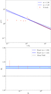Fig. 2. Top panel: Measured correlation function for Lévy flights with α = 1.5, ℓ0 = 0.02 (red points and error bars). The dashed blue line is the expected large r ≫ ℓ0 behaviour ζ(r)∼rα − D, but the actual dependence is slightly steeper, with an effective measured power law α ≃ 1.43 (solid blue line). Bottom panel: Measured Skewness 𝒮3 from Lévy flights with different ξ0 variances (red points and error bars) with α = 3/2. The error bars correspond to the error on the mean from Nreal = 100 realisations each. The BMF prediction yields a better fit to the measured skewness compared to the MF (dashed black line), but there is a slight ambiguity in recovering the exact BMF prediction due to the α dependence of the statistic (cf. solid, dashed blue lines and shaded blue region).

In Fig. 2 (bottom panel) we present 𝒮₃ – the pixel sample skewness for Lévy flights with different ξ₀ variances (red points and error bars). For each ξ₀ value, we generated N_real = 100 realisations and present the mean and the error on the mean of 𝒮₃. The MF limit, and exact BMF expectation values, are presented as dotted black, and dashed or solid blue lines, respectively. The solid blue region represents the uncertainty associated with finite box effects. The means of the simulations agree well with the expected exact solutions, to within ≲0.5% for all variances probed.

The probability distribution functions, P(ρ), are presented in Fig. 3. In the left panels, we present the numerically reconstructed PDFs (red points and error bars), the MF expectation value (14) (dashed black lines), and the BMF prediction constructed in Sect. 3 (solid and dashed blue lines), using the third-order BMF expansion. In the left panels, we present the PDFs, and in the right panels the difference between the numerically reconstructed PDFs and the MF approximation, and the corresponding difference between BMF and MF theoretical expectation (blue lines). The top, middle, and bottom panels correspond to fields with an average variance of ξ₀ = 0.08, 0.88, 2.47, respectively. In the left panels, the points and error bars are the mean and the standard deviations of N_real = 100 realisations. In the right panels, the error bars correspond to the error on the mean. The solid filled blue regions represent the uncertainty associated with finite box effects. We observe that the BMF prediction closely matches the numerical results, even for fully non-Gaussian fields with ξ₀ > 1. The MF approximation fails at low densities, but remains a good fit to the data in the high-density tails.

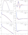Fig. 3. Left: Two-dimensional Lévy flight probability distribution function. Right: difference with respect to the MF with parameters α = 3/2, ξ0 = 0.08, 0.88, 2.47 (top-bottom panels), L = 4000 × Δ (box width), Npts = 40 × 20002 (number of steps), Δ = 0.25 (resolution), and R = 1 (smoothing scale). The error bars show the standard deviation in the left panels and the error on the mean for 100 realisations in the right panels. The points are the sample means. The corresponding standard deviations of the fields are given by ${\sigma }_0=\sqrt{{\xi }_0}=0.28,0.94,1.57$ (top-bottom). The BMF prediction agrees well with the simulations even in the non-perturbative, non-Gaussian regime.

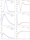Fig. 4. Left: Excursion set perimeter length, W1. Right: Euler characteristic – measured (red points and error bars), mean-field expectation value (dashed black lines) and BMF with α = 1.5 (dashed blue lines) and α = 1.43 (solid blue lines). The error bars represent the standard deviation, and the points are the sample means. The top to bottom panels are the cases ξ0 = 0.08, 0.88, 2.47, respectively, with the parameters Δ = 0.25, R = 1, L = 4000 × Δ, α = 3/2, and Npts = 40 × 20002. Once again the agreement is excellent, especially at the high-density end. Note that the BMF prediction for χ (right panels) is beyond the scope of this paper.

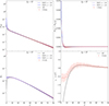Fig. 5. Summary statistics, P(ρ) (top left), W1 (bottom left), and χ (bottom right), for a set of Nreal = 100 realisations of a highly non-Gaussian field with ξ0 = 27 and other parameters of Δ = 0.25, R = 1, L = 4000 × Δ, α = 3/2, and Npts = 40 × 20002. The difference between P(ρ) and the MF prediction is also presented (top right). Error bars show the standard deviation, and the points the sample means. The BMF estimates of the PDF (solid blue lines, top panels) and W1 (bottom left panel) remain an excellent approximation for ξ0 > 20. The MF limit is a good approximation for all statistics in the high-density tails.

There are two other Minkowski functionals associated with a 2D field: the iso-field perimeter length, W₁, and the Euler characteristic, χ. We present these quantities in the left and right panels of Fig. 4, respectively, for the same data used in Fig. 3. Specifically the top, middle, and bottom panels are measurements made from realisations with average field variances ξ₀ = 0.08, 0.88, 2.47, respectively. The red points and error bars are the mean and standard deviations of N_real = 100 Lévy flight realisations. The MF predictions are presented as dashed black lines and the BMF predictions for W₁ are presented as dashed blue (α = 1.5) and solid blue (α = 1.43) lines (left panels). The quantities W₁ and χ depend on the joint probability distribution function for the field ρ and its first and second derivatives. The joint PDF of the field and its first derivatives, and the corresponding BMF prediction for W₁, are presented in Sect. 3 and Appendices A and B. The quantity W₁ depends on both ξ₀ and ξ₁, and we measured the variance of the field, ξ₀, and its gradient, ξ₁, from the simulations and used these values in the analytic form for W₁. Also, we note that W₁ is a dimension-full quantity. Throughout this work, we have chosen the smoothing scale R = 1, so it should be understood that W₁ is presented in units of R pixels.

In the left panels of Fig. 4, we observe that the MF prediction for W₁ (dashed black lines) closely matches the numerical simulations (red points) for small ξ₀ values (cf. top panel) and the large ρ tails for large variance fields (cf. middle, bottom panels). The BMF prediction agrees well with the simulations for practically all densities, even for field variances larger than unity. The right panels present a similar conclusion for χ; both for small ξ₀ fields and the high-density tails of large ξ₀ fields, the MF approximation performs well. The BMF prediction for the joint PDF of the first and second derivatives, required for χ, is left for future work.

In Fig. 5 we present the same statistics as in Figs. 3 and 4, but now taking a set of N_real = 100 highly non-Gaussian Lévy flights with an average variance of ξ₀ = 27. The BMF prediction (blue lines, top and lower left panels) remains an excellent approximation for the numerically reconstructed PDF, and the MF limit is accurate in the high-density tails, ρ ≳ 10. The typical magnitudes of W₁ and χ decrease with increasing ξ₀; this is due to the Lévy flights occupying an increasingly small number of pixels as we decrease ℓ₀. Most of the pixels are zero-density, and as we continue to increase ξ₀ we will encounter issues with the numerical reconstruction, chiefly with the resolution required to resolve the regions containing Lévy flight points. For large values of ξ₀, varying the box size will significantly affect the properties of the field. Decreasing the box size will decrease the number of empty pixels, which will increase the average density and decrease the corresponding variance after ρ is normalised to $\overline{\rho }=1$. Regardless, our numerical reconstructions confirm that the BMF results are accurate even for highly non-Gaussian flights.

5. Conclusion

Rayleigh-Lévy flights belong to a family of point distributions for which the CGF can be exactly calculated in a certain limit – specifically the MF limit – and as such their statistical properties can be explored in the non-perturbatively non-Gaussian regime. In this work we have measured the statistical properties of 2D Rayleigh-Lévy flights, to test the underlying accuracy of the MF and BMF theoretical expectations. For this purpose, we utilised the Minkowski functionals, which are summary statistics that contain non-Gaussian information to all orders in the one-point statistics of the field.

Predictions for the PDF of the density field beyond the MF approximation, obtained by expanding the r-CGF to third order in a Laguerre polynomial basis, were compared to simulations and found to be in agreement at both high and low densities. The PDF was accurately reproduced even for non-perturbatively, non-Gaussian fields with variances larger than unity (Figure 3). Specifically, we confirm that the BMF estimate is accurate over three orders of magnitude for the field variance 10⁻¹ ≲ ξ₀ ≲ 10². Similarly the BMF estimate for W₁ was constructed for the first time and shown to be in agreement with simulated Rayleigh-Lévy flights over the same wide range of field variances. While the BMF prediction for the Minkowski functional, χ, is beyond the scope of this paper, the mean-field predictions for this statistic was also favourably compared to Monte Carlo runs. The MF approximation was found to be a good approximation at intermediate and high densities, even for highly non-Gaussian fields, only failing at low density (Fig. 4). Our precise match to ensembles of simulations highlighted residual biases; for example, ones associated with finite box effects leading to effective values for α as measured via the correlation function that differ from the expected one (Fig. 2).

It would be interesting to extend the 2D measurements to critical points statistics (peaks, voids saddles), following (Bernardeau & Pichon 2024). It would also be of interest to extend the present measurements to 3D flights, though we anticipate that the effect of finite boxes will become more dramatic.

Our results highlight the versatility of Rayleigh-Lévy flights, offering insights not only for astrophysical contexts but also for broader interdisciplinary applications. Rayleigh-Lévy flights model is a unique example of a random process that can both easily be implemented and whose statistical properties are explicitly known (in terms of correlation functions). Furthermore those correlation functions share qualitatively the same properties as those expected for cosmic density fields in both its quasi-linear regime and its strongly non-linear regime. This is therefore a very precious toy model for which analytical methods or numerical tools can be tested, from a departure from Gaussian statistics to the exploration of the fully non-linear regime. For example, one can obtain insights into the validity range of the Edgeworth expansion, which is commonly used to model the perturbative non-Gaussianity of the matter density of the Universe as traced by galaxies. The Edgeworth expansion is not a convergent series, so understanding what variances and density ranges we can use it to model the cosmological density field is an open question. The paper illustrates here that fully non-linear objects such as peaks, critical points, and their correlations, can also be investigated in such a model, challenging and extending the picture that can be drawn from Gaussian fields. Furthermore writing numerical codes to evaluate the number of peaks, droughts, and critical points in a discrete set of strongly correlated points can also be challenging. Having a toy model for which exact results are known is therefore very useful.

Acknowledgments

The authors thank Jose Perico Esguerra for statistical physics insights on Lévy flights. RCB and SA are supported by an appointment to the JRG Program at the APCTP through the Science and Technology Promotion Fund and Lottery Fund of the Korean Government, and was also supported by the Korean Local Governments in Gyeongsangbuk-do Province and Pohang City. SA also acknowledges support from the NRF of Korea (Grant No. NRF-2022R1F1A1061590) funded by the Korean Government (MSIT). CP is partially supported by the grant SEGAL ANR-19-CE31-0017 of the French Agence Nationale de la Recherche. The codes underlying this work are distributed at https://github.com/reggiebernardo/notebooks.

References

Appendix A: Beyond mean field (BMF) calculations in 2D Rayleigh-Lévy flights

We present here the basis for the computation of quantities in the BMF computation for the 2D case. As for the 1D case described in Bernardeau & Pichon (2024), the idea is to project Eq. (8) on a discrete basis. For a Gaussian window function, the eigenfunctions of the 2D harmonic oscillator are a natural choice.

A.1. The field expansion and equations

Following the key equation, Eq. (21), we need to compute Ξ_nn′nc^mm′m_c for the cases of interest. In practice, for the statistics of the density PDF and W₁ we only need to know it for n_c = m_c = 0 and n_c = 0, m_c = ±1 to have access both the density and its gradient. In the following we will give these quantities with its explicit dependence with the sign of m, m′ and m_c that will be denoted ϵ, ϵ′ and ϵ_c, so that below the notations m and m′ should be understood as absolute values. Expressing the two-point function in terms of the power spectrum P(k), defined such that ξ(x) = ∫d²k P(k)exp(ik.x) we have

$$\begin{array}{c}\hfill {\mathrm{\Xi }}_{n{n}^{\prime }0}^{ϵm{ϵ}^{\prime }{m}^{\prime }0}={\displaystyle \int {\mathrm{d}}^2}\mathbf{k}P(k)B_n^{ϵm}(\mathbf{k})B_{n^{\prime }}^{{ϵ}^{\prime }{m}^{\prime }\ast }(\mathbf{k}),\end{array}$$(A.1)

with

$$\begin{array}{cc}\hfill B_n^{ϵm}(\mathbf{k})& ={\displaystyle \int {\mathrm{d}}^2}\mathbf{x}{e}^{\mathrm{i}\mathbf{k}.\mathbf{x}}{\mathcal{C}}_0(\mathbf{x})b_n^{(m)}(\mathbf{x})=c_n^m{\displaystyle \int \mathrm{d}r}{r}^{1+m}{\mathcal{C}}_0(r)L_n^{(m)}(r^2/2){\displaystyle \int \mathrm{d}\theta }{e}^{\mathrm{i}ϵm\theta }{e}^{\mathrm{i}krcos(\theta -{\theta }_k)},\hfill \end{array}$$(A.2a)

$$\begin{array}{cc}\hfill B_n^{ϵm\ast }(\mathbf{k})& ={\displaystyle \int {\mathrm{d}}^2}\mathbf{x}{e}^{-\mathrm{i}\mathbf{k}.\mathbf{x}}{\mathcal{C}}_0(\mathbf{x})b_n^{(m)}(\mathbf{x}),\hfill \end{array}$$(A.2b)

and

$$\begin{array}{c}\hfill {\mathrm{\Xi }}_{n{n}^{\prime }0}^{ϵm{ϵ}^{\prime }{m}^{\prime }{ϵ}_c}={\displaystyle \int {\mathrm{d}}^2}\mathbf{k}P(k)B_n^{ϵm}(\mathbf{k})B_{n^{\prime }}^{{ϵ}^{\prime }{m}^{\prime }{ϵ}_c}(\mathbf{k}),\end{array}$$(A.3)

with

$$\begin{array}{c}\hfill B_n^{ϵm{ϵ}_c}(\mathbf{k})={\displaystyle \int {\mathrm{d}}^2}\mathbf{x}{e}^{-\mathrm{i}\mathbf{k}.\mathbf{x}}{\mathcal{C}}_1^{({ϵ}_c)}(\mathbf{x})b_n^{(m^{\prime })}(\mathbf{x})=c_n^m{\displaystyle \int \mathrm{d}r}{r}^{2+m}{\mathcal{C}}_0(r)L_n^{(m)}(r^2/2){\displaystyle \int \mathrm{d}\theta }{e}^{\mathrm{i}(ϵm+{ϵ}_c)\theta }{e}^{-\mathrm{i}krcos(\theta -{\theta }_k)}.\end{array}$$(A.4)

The expressions of the normalisation coefficients c_n^m can easily be obtained from (17) and they read

$$\begin{array}{c}\hfill c_n^m=1/\sqrt{\frac{2^m(m+n)!}{n!}}.\end{array}$$(A.5)

The integration over the angle θ yields a Bessel function of order m, and the final result reads

$$\begin{array}{cc}\hfill B_n^{ϵm}(\mathbf{k})& =c_n^m\frac{e^{-\frac{k^2}{2}}{k}^{m+2n}}{(2n)\text{!!}}{\mathrm{i}}^m{e}^{\mathrm{i}ϵm{\theta }_k},\hfill \end{array}$$(A.6a)

$$\begin{array}{cc}\hfill B_n^{ϵm\ast }(\mathbf{k})& =c_n^m\frac{e^{-\frac{k^2}{2}}{k}^{m+2n}}{(2n)\text{!!}}{\mathrm{i}}^{-m}{e}^{\mathrm{i}ϵm{\theta }_k},\hfill \end{array}$$(A.6b)

$$\begin{array}{cc}\hfill B_n^{ϵm{ϵ}_c}(\mathbf{k})& =c_n^m\frac{e^{-\frac{k^2}{2}}{k}^{m+2n}(-2n+(ϵ{ϵ}_c-1)m+k^2)}{(2n)\text{!!}}{\mathrm{i}}^{-1-m}{e}^{-\mathrm{i}(ϵm+{ϵ}_c){\theta }_k}.\hfill \end{array}$$(A.6c)

We can also express the result for a power law correlation function, or equivalently while assuming that the spectrum follows a power law in P(k) = A k^n_s.

For the function W₁(ρ), we need to build the CGF of the density and its gradient along a given direction, say Ox. The CGF will then be symmetric with respect to the Oy axis. Then it suffices to restrict our basis to symmetric functions, that is to use

$$\begin{array}{c}\hfill b_n^{(m)}(\mathbf{x})=\sqrt{2}{c}_n^m{L}_n^{(m)}(r^2/2)r^{m}cos(m\theta ),\end{array}$$(A.7)

and 𝒞₁(x) = 𝒞₀(r) r cos(θ). With this definition of functions, Eq. (21) becomes

$$\begin{array}{cc}\hfill {\mathrm{\Xi }}_{n{n}^{\prime }0}^{m{m}^{\prime }0}& ={\xi }_0\frac{\mathrm{\Gamma }(1+n_s/2+n+n^{\prime }+(m+m^{\prime })/2)}{(2n)\text{!!}\sqrt{\frac{2^m(m+n)!}{n!}}\left(2n^{\prime }\right)\text{!!}\sqrt{\frac{2^{m^{\prime }}(m^{\prime }+n^{\prime })!}{n^{\prime }!}}\mathrm{\Gamma }(\frac{n_s}{2}+1)}{\delta }_m^{m^{\prime }},\hfill \end{array}$$(A.8a)

$$\begin{array}{cc}\hfill {\mathrm{\Xi }}_{n{n}^{\prime }0}^{m{m}^{\prime }1}& ={\xi }_0{c}_{m+m^{\prime }}\frac{((m-m^{\prime })(n_s+2n-2n^{\prime })+(m^{\prime }+m)+1)\mathrm{\Gamma }(n_s/2+n+n^{\prime }+(m+m^{\prime }+1)/2)}{4(2n)\text{!!}\sqrt{\frac{2^m(m+n)!}{n!}}\left(2n^{\prime }\right)\text{!!}\sqrt{\frac{2^{m^{\prime }}(m^{\prime }+n^{\prime })!}{n^{\prime }!}}\mathrm{\Gamma }(\frac{n_s}{2}+1)}{\delta }_{|m^{\prime }-m|}^1,\hfill \end{array}$$(A.8b)

with ${\xi }_0={\mathrm{\Xi }}_{000}^{000}$, and

$$\begin{array}{c}\hfill c_{m+m^{\prime }}=\text{if}\left[\begin{array}{cc}m+m^{\prime }=1,& \sqrt{2}\\ m+m^{\prime }>1,& 1\end{array}\right].\end{array}$$(A.9)

Numerical solutions were used to fix the normalisation. These results can be checked by direct numerical integrations of the weighted correlation function.

A.2. BMF density CGFs and skewness

With the help of the previous result, we can easily derive the resulting CGFs. It only requires to solve the system (20) for a chosen order. We choose here to truncate the expansion for a fixed n_t. For the CGF of the density only, it means that BMF results change for even indices. For the CGF for both the density and density gradient, it changes at all order.

Some results are presented in the main text. We complement here results obtained for higher orders. For α = 3/2, the one-point density CGF with third-order polynomial corrections beyond the MF [symbolically, τ(x)≡τ₀⁰ + τ₁⁰b₁⁽⁰⁾(x)+τ₂⁰b₂⁽⁰⁾(x)+τ₃⁰b₃⁽⁰⁾(x)] is given by

$$\begin{array}{cc}\hfill {\phi }_6(\lambda )& =-\frac{\lambda (14625{\lambda }^3{\xi }_0^3-37299300{\lambda }^2{\xi }_0^2+4671569920\lambda {\xi }_0-68719476736)}{4800{\lambda }^4{\xi }_0^4-14061665{\lambda }^3{\xi }_0^3+2074748004{\lambda }^2{\xi }_0^2-39031308288\lambda {\xi }_0+68719476736}.\hfill \end{array}$$(A.10)

For an arbitrary power law correlation function ξ(r) = 1/r^β the CGF φ₄(λ) is given by

$$\begin{array}{cc}\hfill {\phi }_4(\lambda )& =\frac{\lambda (\beta (\beta +2)\lambda {\xi }_0(16(\beta (\beta +10)+88)-\beta (\beta +2)(\beta +4)\lambda {\xi }_0)-32768)}{\lambda {\xi }_0(\beta (4\beta (\beta +2){\lambda }^2{\xi }_0^2-(\beta (\beta (\beta (\beta +8)+84)+336)+1408)\lambda {\xi }_0+16(\beta +2)(\beta (\beta +10)+88))+16384)-32768}.\hfill \end{array}$$

CGFs with higher order BMF corrections can be obtained, but are unwieldy to print. Nonetheless, these can be calculated and stored using algebraic computing softwares such as Mathematica. For this work, we have evaluated up to φ₆(λ) for fixed-α cases (e.g., α = 1/2, 3/2) and up to φ₄(λ) for the arbitrary power law correlation.

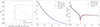Fig. A.1. Skewness in 2D Lévy flight distribution in the BMF formalism (left) as a function of the order of the expansion in (18) for α = 3/2 and (middle) as a function of the Lévy flight index α. Exact and MF values are shown as red-solid and black-dotted lines, respectively. (Right) The difference between MF and BMF density probability distribution functions for different expansion orders. We present the PDF from the main body of the text; ξ0 = 2.47 and use an effective α = 1.43 in the BMF expansion. The red points/error bars are the mean and error on mean of the simulated flights.

The skewness obtained for CGFs with increasing order of corrections BMF are shown in Fig. A.1, supporting an exponential convergence of the BMF formalism to the exact solution.

A.3. BMF joint density and density gradient CGF

The first non trivial result is obtained for α = 3/2 and when we restrict to n_t = 1, that is when the first two functions of the basis only are used, is given by

$$\begin{array}{c}\hfill {\phi }_1(\lambda ,{\lambda }_x)=\frac{16(16\lambda +{\xi }_0({\lambda }_x^2-{\lambda }^2))}{{\xi }_0^2(8{\lambda }^2-7{\lambda }_x^2)+256-144\lambda {\xi }_0}.\end{array}$$(A.11)

Its counterpart for any correlation index β is given by Eq. (26) in the main text, taking advantage of the fact that all correlators are explicitly known. The next interesting order is n_t = 3. At such order we can include the next basis element for m = 1. Note that to be consistent, there are in total six basis elements to include, n = 0 and 1 for m = 0 and 1 and n = 0 for m = 2 and m = 3. For α = 3/2, the result takes the form

$$\begin{array}{cc}\hfill {\phi }_3(\lambda ,{\lambda }_x)& =\frac{P(\lambda ,{\lambda }_x)}{Q(\lambda ,{\lambda }_x)},\mathrm{where}\hfill \\ \hfill P(\lambda ,{\lambda }_x)& =4(7.03687\times {10}^{13}\lambda +2.51658\times {10}^8\lambda {\xi }_0^2(2061{\lambda }^2-1880{\lambda }_x^2)\hfill \\ \hfill & -1.37439\times {10}^{11}{\xi }_0(77{\lambda }^2-32{\lambda }_x^2)+500\lambda {\xi }_0^4(168832{\lambda }^4-522016{\lambda }^2{\lambda }_x^2+183207{\lambda }_x^4)\hfill \\ \hfill & -204800{\xi }_0^3(50344{\lambda }^4-87243.{\lambda }^2{\lambda }_x^2+9792{\lambda }_x^4)-1875{\xi }_0^5(128{\lambda }^6-608{\lambda }^4{\lambda }_x^2+513{\lambda }^2{\lambda }_x^4-105{\lambda }_x^6)),\hfill \\ \hfill Q(\lambda ,{\lambda }_x)& =6.71089\times {10}^7{\xi }_0^2(329923{\lambda }^2-123944{\lambda }_x^2)\hfill \\ \hfill & -1.83069\times {10}^{14}\lambda {\xi }_0-32768\lambda {\xi }_0^3(2.918\times {10}^7{\lambda }^2-2.57737\times {10}^7{\lambda }_x^2)\hfill \\ \hfill & -100\lambda {\xi }_0^5(1.38483\times {10}^6{\lambda }^4-4.16963\times {10}^6{\lambda }^2{\lambda }_x^2+1.45172\times {10}^6{\lambda }_x^4)\hfill \\ \hfill & +240{\xi }_0^4(7.34829\times {10}^7{\lambda }^4-1.24732\times {10}^8{\lambda }^2{\lambda }_x^2+1.41909\times {10}^7{\lambda }_x^4)\hfill \\ \hfill & +375{\xi }_0^6(1024{\lambda }^6-4736{\lambda }^4{\lambda }_x^2+3912{\lambda }^2{\lambda }_x^4-795{\lambda }_x^6)+2.81475\times {10}^{14}.\hfill \end{array}$$(A.12)

This is the form used in practice to compare with simulations in the computation of the W₁ indicator.

Appendix B: Derivation of W₁(ρ) as a function of the CGF

The iso-field perimeter, W₁, is given in general by Eq. (27)

$$\begin{array}{c}\hfill W_1(\rho )={\displaystyle \int \int \sqrt{{\rho }_x^2+{\rho }_y^2}}\mathrm{d}{\rho }_x\mathrm{d}{\rho }_{y}P(\rho ,{\rho }_x,{\rho }_y),\end{array}$$(B.1)

where the PDF, P(ρ, ρ_x, ρ_y), can be expressed as

$$\begin{array}{c}\hfill P(\rho ,{\rho }_x,{\rho }_y)={\displaystyle \int \frac{\mathrm{d}{\lambda }_{\rho }}{2\pi \mathrm{i}}\int \frac{\mathrm{d}{\lambda }_x}{2\pi \mathrm{i}}\int \frac{\mathrm{d}{\lambda }_y}{2\pi \mathrm{i}}}exp(-{\lambda }_{\rho }\rho -{\lambda }_x{\rho }_x-{\lambda }_y{\rho }_y+\phi (\lambda ,{\lambda }_x,{\lambda }_y)),\end{array}$$(B.2)

in terms of φ(λ, λ_x, λ_y), the joint CGF for ρ, ρ_x and ρ_y. After integration by parts, Eq. (B.2) becomes

$$\begin{array}{c}\hfill P(\rho ,{\rho }_x,{\rho }_y)={\displaystyle \int \frac{\mathrm{d}{\lambda }_{\rho }}{2\pi \mathrm{i}}\int \frac{\mathrm{d}{\lambda }_x}{2\pi \mathrm{i}}\int \frac{\mathrm{d}{\lambda }_y}{2\pi \mathrm{i}}}\frac{1}{{\rho }_x}\frac{\partial \phi }{\partial {\lambda }_x}exp(-{\lambda }_{\rho }\rho -{\lambda }_x{\rho }_x-{\lambda }_y{\rho }_y+\phi (\lambda ,{\lambda }_x,{\lambda }_y)).\end{array}$$(B.3)

The integration element dρ_xdρ_y and dλ_xdλ_y in Eqs. (B.1) and (B.2) can be written respectively in polar co-ordinates as ρ_gdρ_gdθ_g and λ_gdλ_gdθ_λ. We further take advantage of the fact that φ(λ, λ_x, λ_y) is a function of λ_g² ≡ λ_x² + λ_y² only so that

$$\begin{array}{c}\hfill \frac{\partial \phi }{\partial {\lambda }_x}=\frac{{\lambda }_x}{{\lambda }_g}\frac{\partial \phi }{\partial {\lambda }_g}.\end{array}$$(B.4)

This implies that Eq. (B.1) can we re-expressed explicitly in terms of the CGF as

$$\begin{array}{c}\hfill W_1={\displaystyle \int \int \int \frac{\mathrm{d}{\lambda }_{\rho }}{2\pi \mathrm{i}}}\frac{{\lambda }_g\mathrm{d}{\lambda }_g\mathrm{d}{\theta }_{\lambda }}{2{\pi }^2}{\displaystyle \int \int {\rho }_g^2}\mathrm{d}{\rho }_g\mathrm{d}{\theta }_g\frac{1}{{\rho }_{g}cos{\theta }_g}\frac{{\lambda }_{g}cos{\theta }_{\lambda }}{{\lambda }_g}\frac{\partial \phi ({\lambda }_{\rho },{\lambda }_g)}{\partial {\lambda }_g}exp(-{\lambda }_{\rho }\rho -{\lambda }_g{\rho }_{g}cos({\theta }_{\lambda }-{\theta }_g)+\phi (\lambda ,{\lambda }_g)).\end{array}$$(B.5)

The integral over θ_λ in Eq. (B.5) gives

$$\begin{array}{c}\hfill {\displaystyle \int \mathrm{d}}{\theta }_{\lambda }cos{\theta }_{\lambda }exp({\lambda }_g{\rho }_{g}cos({\theta }_{\lambda }-{\theta }_g))=-2\pi \mathrm{i}{J}_1({\lambda }_g{\rho }_g)cos{\theta }_g.\end{array}$$(B.6)

Using then the fact that

$$\begin{array}{c}\hfill J_1({\lambda }_g{\rho }_g)=-\frac{1}{{\rho }_g}\frac{\mathrm{d}}{\mathrm{d}{\lambda }_g}{J}_0({\lambda }_g{\rho }_g),\mathrm{and}{\displaystyle {\int }_0^{\infty }}\mathrm{d}{\rho }_g{J}_0({\lambda }_g{\rho }_g)=\frac{1}{{\lambda }_g},\end{array}$$(B.7)

allows us to carry out the integration over ρ_g and θ_g, so that W₁ becomes

$$\begin{array}{c}\hfill W_1=-{\displaystyle {\int }_{-\mathrm{i}\infty }^{+\mathrm{i}\infty }}\frac{\mathrm{d}{\lambda }_{\rho }}{2\pi }{\displaystyle {\int }_0^{\infty }}\frac{\mathrm{d}{\lambda }_g}{{\lambda }_g}\frac{\partial \phi ({\lambda }_{\rho },{\lambda }_g)}{\partial {\lambda }_g}exp(-{\lambda }_{\rho }\rho +\phi ({\lambda }_{\rho },{\lambda }_g)),\end{array}$$(B.8)

which in practice can be rewritten as Eq. (30) (given in the main text), after a further integration by parts.

Appendix C: Numerical algorithms and testing

In this section we briefly describe the numerical algorithms used to generate the density field PDF and Minkowski Functional curves. Lévy flights are generated sequentially as point distributions that are binned onto a regular lattice using a nearest neighbour scheme. Throughout this work we take a regularly spaced lattice with N = 4000 points per side and resolution Δ = 0.25, generating a box length L = 4000 × Δ = 1000. Periodic boundary conditions are enforced modulo L at each step of the flight, imposing periodic boundary conditions on the resulting field.

The density field constructed by binning the flight is subjected to a discrete Fourier transform, then smoothed in Fourier space using a kernel W(kR) = exp[−k²R²/2] and inverse Fourier transformed. The smoothing scale is always set to be R = 1, to match the Gaussian filter used in the theoretical calculations. From these fields we extract the summary statistics presented in the main body of the text. The PDF of the field is estimated by binning the pixels into a ρ_i array, and then normalising the resulting histogram to unity. We take N = 500, ρ_i values regularly spaced over 0 < ρ ≤ 10, except for the case ξ₀ = 27 in which case we use N = 1200 values regularly spaced over 0 < ρ ≤ 80.

The Minkowski Functionals W₁ and χ are extracted from the field by taking the array of density threshold values ρ_i, and generating iso-field boundaries for each threshold. A constant field boundary is a 1D curve, which is generated using the marching squares algorithm as detailed in Appleby et al. (2018). In short, the algorithm linearly interpolates between adjacent values of the density field on the lattice according to a scheme that creates a set of closed polygons. W₁ is then the total length of the line segments that make up the polygons, and we define the genus W₂ as the sum of rotation angles along the iso-field lines, divided by 2π. The Euler characteristic χ is then the derivative of W₂ with respect to ρ_i; we use the central derivative scheme χ_i = (W_{2, i + 1} − W_{2, i − 1})/(ρ_i + 1 − ρ_i − 1). Both W₁ and χ are defined here as densities, so they are normalised by the area of the box.

C.1. Gaussian random fields

To assess the accuracy of the algorithms adopted, we extract the Minkowski Functionals from fields for which exact expectation values are known. We cannot use Lévy flights with large ξ₀ variances to test the numerics in this way because their expectation values are not exactly known; they are subject to BMF corrections and the convergence of this approximation to the exact properties of the field is unknown. In this appendix we generate Gaussian random fields, for which the ensemble expectation values for P(ρ), W₁ and χ are exactly known. This allows us to quantify the numerical limits of our methodology, at least for fields that are close to Gaussian.

In Fig. C.1 we present the summary statistics P, W₁, χ extracted from N_real = 50 realisations of a Gaussian random field. Red points/errorbars are the sample means and error on the means of the realisations. Specifically, the Gaussian random fields are drawn in Fourier space from a white noise power spectrum P(k)∝kⁿe^−k2R2 with n = 0 and the same parameters as the main body of the text; R = 1, Δ = 0.25, L = 4000 × Δ. After inverse fast Fourier transforming, the density field is mean subtracted and normalised to unit variance; $\nu =(\rho -\overline{\rho })/\sqrt{{\xi }_0}$. For Gaussian fields, the PDF and Minkowski Functionals have the exact ensemble expectation values

$$\begin{array}{c}\hfill P(\nu )=\frac{1}{\sqrt{2\pi }}{e}^{-{\nu }^2/2},W_1(\nu )=\frac{1}{2}\sqrt{\frac{{\xi }_1}{2{\xi }_0}}{e}^{-{\nu }^2/2},\chi (\nu )=\frac{1}{{(2\pi )}^{3/2}}\frac{{\xi }_1}{2{\xi }_0}{e}^{-{\nu }^2/2}({\nu }^2-1).\end{array}$$(C.1)

We compare the numerically extracted statistics (red points/error bars) to the Gaussian expectation (black dashed lines). The sub-panels show ΔP, ΔW₁ and Δχ; the differences between theoretical predictions and simulated measurements for each statistic (red points/error bars). For each statistic, the simulation measurements successfully reproduce the predictions to sub-percent level. W₁ is the only statistic that exhibits any systematic offset (cf middle panel); this is because the linear interpolation approximation of a smooth curve neglects curvature at the resolution scale. Even for W₁, the systematic offset between numerical reconstruction and prediction ≲0.5% for all densities.

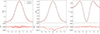Fig. C.1. Summary statistics (PDF, W1, χ) extracted from Gaussian random fields (left, middle, right panels). The red points/errorbars are measured from simulations and the black dashed lines are the expectation values. The lower sub-panels show the difference between measurements and theory.

All Figures

	Fig. 1. Two-dimensional Rayleigh-Lévy flight with parameters α = 3/2 and ξ0 ∼ 2.47 (ℓ0 = 0.01), a density of Npts = 40 points per pixel, a box width of L = 4000 × Δ, a resolution of Δ = 0.25, and a Gaussian smoothing scale of R = 1.
In the text

Fig. 2. Top panel: Measured correlation function for Lévy flights with α = 1.5, ℓ0 = 0.02 (red points and error bars). The dashed blue line is the expected large r ≫ ℓ0 behaviour ζ(r)∼rα − D, but the actual dependence is slightly steeper, with an effective measured power law α ≃ 1.43 (solid blue line). Bottom panel: Measured Skewness 𝒮3 from Lévy flights with different ξ0 variances (red points and error bars) with α = 3/2. The error bars correspond to the error on the mean from Nreal = 100 realisations each. The BMF prediction yields a better fit to the measured skewness compared to the MF (dashed black line), but there is a slight ambiguity in recovering the exact BMF prediction due to the α dependence of the statistic (cf. solid, dashed blue lines and shaded blue region).

In the text

Fig. 3. Left: Two-dimensional Lévy flight probability distribution function. Right: difference with respect to the MF with parameters α = 3/2, ξ0 = 0.08, 0.88, 2.47 (top-bottom panels), L = 4000 × Δ (box width), Npts = 40 × 20002 (number of steps), Δ = 0.25 (resolution), and R = 1 (smoothing scale). The error bars show the standard deviation in the left panels and the error on the mean for 100 realisations in the right panels. The points are the sample means. The corresponding standard deviations of the fields are given by ${\sigma }_0=\sqrt{{\xi }_0}=0.28,0.94,1.57$ (top-bottom). The BMF prediction agrees well with the simulations even in the non-perturbative, non-Gaussian regime.

In the text

Fig. 4. Left: Excursion set perimeter length, W1. Right: Euler characteristic – measured (red points and error bars), mean-field expectation value (dashed black lines) and BMF with α = 1.5 (dashed blue lines) and α = 1.43 (solid blue lines). The error bars represent the standard deviation, and the points are the sample means. The top to bottom panels are the cases ξ0 = 0.08, 0.88, 2.47, respectively, with the parameters Δ = 0.25, R = 1, L = 4000 × Δ, α = 3/2, and Npts = 40 × 20002. Once again the agreement is excellent, especially at the high-density end. Note that the BMF prediction for χ (right panels) is beyond the scope of this paper.

In the text

Fig. 5. Summary statistics, P(ρ) (top left), W1 (bottom left), and χ (bottom right), for a set of Nreal = 100 realisations of a highly non-Gaussian field with ξ0 = 27 and other parameters of Δ = 0.25, R = 1, L = 4000 × Δ, α = 3/2, and Npts = 40 × 20002. The difference between P(ρ) and the MF prediction is also presented (top right). Error bars show the standard deviation, and the points the sample means. The BMF estimates of the PDF (solid blue lines, top panels) and W1 (bottom left panel) remain an excellent approximation for ξ0 > 20. The MF limit is a good approximation for all statistics in the high-density tails.

In the text

Fig. A.1. Skewness in 2D Lévy flight distribution in the BMF formalism (left) as a function of the order of the expansion in (18) for α = 3/2 and (middle) as a function of the Lévy flight index α. Exact and MF values are shown as red-solid and black-dotted lines, respectively. (Right) The difference between MF and BMF density probability distribution functions for different expansion orders. We present the PDF from the main body of the text; ξ0 = 2.47 and use an effective α = 1.43 in the BMF expansion. The red points/error bars are the mean and error on mean of the simulated flights.

In the text

	Fig. C.1. Summary statistics (PDF, W1, χ) extracted from Gaussian random fields (left, middle, right panels). The red points/errorbars are measured from simulations and the black dashed lines are the expectation values. The lower sub-panels show the difference between measurements and theory.
In the text

References

- Appleby, S., Chingangbam, P., Park, C., et al. 2018, ApJ, 858, 87 [Google Scholar]
- Bardeen, J. M., Bond, J. R., Kaiser, N., & Szalay, A. S. 1986, ApJ, 304, 15 [Google Scholar]
- Bernardeau, F. 2022, A&A, 663, A124 [NASA ADS] [CrossRef] [EDP Sciences] [Google Scholar]
- Bernardeau, F., & Pichon, C. 2024, A&A, 689, A105 [NASA ADS] [CrossRef] [EDP Sciences] [Google Scholar]
- Bernardeau, F., Colombi, S., Gaztañaga, E., & Scoccimarro, R. 2002, Phys. Rep., 367, 1 [Google Scholar]
- Bond, J. R., Kofman, L., & Pogosyan, D. 1996, Nature, 380, 603 [NASA ADS] [CrossRef] [Google Scholar]
- Cadiou, C., Pichon, C., Codis, S., et al. 2020, MNRAS, 496, 4787 [Google Scholar]
- Fry, J. N. 1985, ApJ, 289, 10 [NASA ADS] [CrossRef] [Google Scholar]
- Gay, C., Pichon, C., & Pogosyan, D. 2012, Phys. Rev. D, 85, 023011 [NASA ADS] [CrossRef] [Google Scholar]
- Holtsmark, J. 1919, Ann. Phys. (Berl.), 363, 577 [Google Scholar]
- Klages, R., Radons, G., & Sokolov, I. M., eds. 2008, Anomalous Transport (Wiley) [Google Scholar]
- Krapivsky, P. L., Redner, S., & Ben-Naim, E. 2010, A Kinetic View of Statistical Physics (Cambridge University Press) [Google Scholar]
- Litovchenko, V. A. 2021, Ukr. Math. J., 73, 76 [Google Scholar]
- Mandelbrot, B. 1975, Acad. Sci. Paris C. R. Serie Sci. Math., 280, 1551 [Google Scholar]
- Matsubara, T. 1994, ApJ, 434, L43 [NASA ADS] [CrossRef] [Google Scholar]
- Mecke, K. R., Buchert, T., & Wagner, H. 1994, A&A, 288, 697 [NASA ADS] [Google Scholar]
- Peebles, P. J. E. 1980, The Large-Scale Structure of the Universe (Princeton University Press) [Google Scholar]
- Peebles, P. J. E., & Groth, E. J. 1975, ApJ, 196, 1 [NASA ADS] [CrossRef] [Google Scholar]
- Pranav, P., Edelsbrunner, H., van de Weygaert, R., et al. 2017, MNRAS, 465, 4281 [Google Scholar]
- Press, W. H., & Schechter, P. 1974, ApJ, 187, 425 [Google Scholar]
- Szapudi, I., & Colombi, S. 1996, ApJ, 470, 131 [NASA ADS] [CrossRef] [Google Scholar]
- Uchaikin, V. V. 2019, Phys. Astron. Int. J., 3, 82 [CrossRef] [Google Scholar]
- White, S. D. M. 1979, MNRAS, 186, 145 [NASA ADS] [CrossRef] [Google Scholar]