| Issue |
A&A
Volume 705, January 2026
|
|
|---|---|---|
| Article Number | A44 | |
| Number of page(s) | 11 | |
| Section | The Sun and the Heliosphere | |
| DOI | https://doi.org/10.1051/0004-6361/202556097 | |
| Published online | 06 January 2026 | |
Multi-height probing of horizontal flows in the solar photosphere
1
Astronomical Observatory, Volgina 7, 11060 Belgrade, Serbia
2
Institute for Solar Physics, Georges-Khöler-Alee 401a, 79110 Freiburg, Germany
3
Department of Astronomy, Faculty of Mathematics, University of Belgrade, Studentski Trg 16-20, 11000 Belgrade, Serbia
4
High Altitude Observatory, NSF National Center for Atmospheric Research, Boulder, CO 80307, USA
5
Natural and Applied Sciences, University of Wisconsin – Green Bay, 2420 Nicolet Drive, Green Bay, WI 54311, USA
6
Laboratory for Atmospheric and Space Physics, University of Colorado, Boulder, CO 80303, USA
7
Department of Astrophysical and Planetary Sciences, University of Colorado Boulder, 2000 Colorado Avenue, Boulder, CO 80305, USA
8
National Solar Observatory, 3665 Discovery Drive, Boulder, CO 80303, USA
9
Instituto de Astrofísica de Canarias (IAC), Avda Vía Láctea s/n, 38200 La Laguna, Tenerife, Spain
10
Departamento de Astrofísica, Universidad de La Laguna, 38205 La Laguna, Tenerife, Spain
11
Environment and Climate Change Canada, Science and Technology Branch, Meteorological Research Division, 2121 Transcanada Hwy, Dorval, Québec H9P 1J3, Canada
★ Corresponding author: This email address is being protected from spambots. You need JavaScript enabled to view it.
Received:
25
June
2025
Accepted:
20
October
2025
Abstract
Context. Optical flow methods aim to infer horizontal (transverse, in the general case) velocities in the solar atmosphere from the temporal changes in maps of physical quantities, such as intensity or magnetic field. So far, these methods have mostly been tested and applied to the continuum intensity and line-of-sight (LOS) magnetic field in the low to mid-photosphere.
Aims. We tested whether simultaneous spectropolarimetric imaging in two magnetically sensitive optical spectral lines, which probe two different layers of the solar atmosphere (the photosphere and the temperature minimum), can help constrain the depth variation of horizontal flows.
Methods. We first tested the feasibility of our method using Fourier local correlation tracking (FLCT) to track physical quantities at different optical depths (log τ500 = −1, −2, −3, −4) in an atmosphere simulated with the MURaM code. We then inferred the horizontal distribution of the LOS magnetic field component from synthetic spectropolarimetric observations of Fe I 525.0 nm and Mg I b2 spectral lines, applied FLCT to the time sequence of these synthetic magnetograms, and compared our findings with the original height-dependent horizontal velocities.
Results. Tracking the LOS magnetic field component (which coincides with the vertical component at the disk center) yields horizontal velocities that, after appropriate temporal and spatial averaging, agree excellently with the horizontal component of the simulated velocities, both calculated at constant τ500 surfaces, up to the temperature minimum (log τ500 = −3). When tracking the temperature at constant τ500 surfaces, this agreement already breaks down completely at the mid photosphere (log τ500 = −2). Tracking the vertical component of the magnetic field inferred from synthetic observations of the Fe I 525.0 nm and the Mg I b2 spectral lines yields a satisfactory inference of the horizontal velocities in the mid-photosphere (log τ500 ≈ −1) and the temperature minimum (log τ500 ≈ −3), respectively.
Conclusions. Our results indicate that high-spatial-resolution spectropolarimetric imaging in solar spectral lines can provide meaningful information about the horizontal plasma velocities over a range of heights.
Key words: Sun: atmosphere / Sun: magnetic fields / Sun: photosphere
© The Authors 2026
 Open Access article, published by EDP Sciences, under the terms of the Creative Commons Attribution License (https://creativecommons.org/licenses/by/4.0), which permits unrestricted use, distribution, and reproduction in any medium, provided the original work is properly cited.
This article is published in open access under the Subscribe to Open model. This email address is being protected from spambots. You need JavaScript enabled to view it. to support open access publication.
1. Introduction
The structure and dynamics of the solar lower atmosphere are driven by interaction between plasma motions and the magnetic field on various spatial scales. In the quiet Sun (QS), in weakly magnetized regions where the magnetic field strength is often below the equipartition value between the magnetic and dynamic pressure (i.e., well below 1 kG), the magnetic field structure is largely determined by plasma motions. By probing plasma dynamics, we can understand the transport and amplification of the magnetic field, as described by the induction equation for an ideal, infinitely conducting fluid:
 (1)
(1)
where v is the velocity vector and B is the magnetic field vector. Therefore, the velocity field is a crucial parameter for understanding solar magnetism on various scales, including, but not limited to, mean-field theories of the solar dynamo (e.g., Charbonneau 2010), small-scale dynamo processes (e.g., Rempel 2014), energy transport from the photosphere upward (Welsch 2015; Tilipman et al. 2023), and magnetohydrodynamic (MHD) wave studies (Skirvin et al. 2024). Estimating plasma velocities also allows us to quantify the energy and mass transport associated with various scales of solar convection (e.g., Nordlund et al. 2009), waves (e.g., Arregui 2015), or swirls (Liu et al. 2019).
The line-of-sight (LOS) component of the plasma velocity is typically estimated from the Doppler effect by using simple line core fitting, bisector techniques, or spectropolarimetric inversion techniques, which provide depth-dependent variations of velocity and other physical parameters (e.g., de la Cruz Rodríguez & van Noort 2017). The transverse velocity component (corresponding to horizontal motions at the disk center) is often probed through optical flows. The term optical flow, originally coined for computer vision applications (see the discussion in Schuck 2006), refers to the apparent motion of a feature, inferred from images taken at different times (Chae & Sakurai 2008). Hence, tracking optical flows involves using one or more techniques to recover the transverse velocity field of the plasma. To derive horizontal velocities using tracking methods, a time series of continuum intensity images or LOS magnetograms (maps of the magnetic field BLOS at different times) is required (Welsch et al. 2007; Verma et al. 2013). The choice between the two is often based on where the tracking is performed (e.g., quiet Sun versus active regions). Over the years, various methods for tracking flows have been developed, but the most commonly used and well-known optical flow method is local correlation tracking (LCT; November & Simon 1988). As the name suggests, it is a local method: the velocity at a given pixel is based on image values within a small area centered on that pixel (Chae & Sakurai 2008).
Fourier local correlation tracking (FLCT; Welsch et al. 2004; Fisher & Welsch 2008), that is, the use of Fourier techniques to calculate correlations, is a faster and more accurate variation of LCT that has been widely applied in solar atmosphere diagnostics. For example, Welsch et al. (2004) applied FLCT to measure the rate of magnetic helicity injected into the corona through the photosphere. Liu et al. (2019) applied FLCT to intensity images obtained by the Solar Optical Telescope (SOT) aboard the Hinode satellite to infer the average radius and rotation speed of photospheric and chromospheric swirls. Moreover, Li et al. (2021) used FLCT to estimate the velocities of supra-arcade downflows (SADs), the plasma voids associated with flare loops. Fisher et al. (2020) used the FLCT code to determine horizontal velocities and their contribution to the noninductive electric field as part of their PTD-Doppler-FLCT-Ideal (where PTD stands for poloidal-toroidal decomposition) software library, PDFI_SS, which computes the electric field at the Sun’s photosphere (Kazachenko et al. 2014; Lumme et al. 2019).
Multiple studies have benchmarked the performance of the LCT and FLCT techniques by applying them to synthetic intensity maps and magnetograms produced by various magnetohydrodynamic (MHD) simulations of the solar photosphere (see, e.g., Rieutord et al. 2001; Verma et al. 2013; Kazachenko et al. 2014; Tremblay et al. 2018; Afanasyev et al. 2021). These benchmarks aim to synthesize observables, apply tracking techniques to them, and compare the results with the original horizontal velocities. For example, Löptien et al. (2016) explained some of the biases in LCT techniques by applying FLCT to continuum images obtained with the Helioseismic and Magnetic Imager (HMI) on board the Solar Dynamics Observatory (SDO; Schou et al. 2012) and to images generated from STAGGER code simulations (Stein 2012), showing that both exhibit a shrinking-Sun effect of comparable magnitude. The term “Shrinking-Sun” refers to a systematic error that appears as a flow converging towards the disk center, which is superimposed on real flows and can reach up to 1 km/s. In general, these benchmarks focus on applying FLCT either to continuum images or to photospheric magnetograms.
In this work, we test the feasibility of recovering plasma flows at multiple atmospheric heights, from the base of the photosphere to the temperature minimum. To this end, we applied FLCT to the time series of the simulated continuum intensity, temperature, T, and the vertical component of the magnetic field, Bz at multiple optical depths, from log τ500 = 0 to log τ500 = −4, and compared the resulting velocities with the original simulation values. We then repeated the same test by tracking magnetograms inferred from synthetic observations of the neutral iron line at 525.02 nm and the b2 line of neutral magnesium at 517.2 nm, which probe the mid-photosphere (log τ500 ≈ −1) and the temperature minimum (log τ500 ≈ −3), respectively. The motivation for using spectral lines lies in their sensitivity to different depths in the solar atmosphere. Specifically, the monochromatic absorption coefficient of the solar plasma increases rapidly with wavelength toward the line center, with substantial changes occurring on picometer scales. This leads to different formation heights for radiation observed at the continuum and line wavelengths. Therefore, interpreting time-dependent multi-line observations using spectropolarimetric inversions (de la Cruz Rodríguez & van Noort 2017) should allow tracking of flows across different layers of the solar atmosphere (different values of optical depth τ500, i.e., height z). Spectral lines also provide a means to infer the LOS velocity through the Doppler effect, and thus probe all three components of the velocity vector. This is especially important in the context of existing and upcoming high-resolution observations of the solar atmosphere obtained with imaging spectropolarimeters such as SST/CRISP (Scharmer et al. 2008), SUNRISE/TuMag (del Toro Iniesta et al. 2025), and DKIST/VTF (Schmidt et al. 2016), or with integral field units such as Microlensed Hyperspectral Imager (MiHI; van Noort et al. 2022) or Helium Spectropolarimeter (HeSP, see Leenaarts et al. 2025). Both the creation and interpretation of spectropolarimetric data, and the analysis of multi-height flows, distinguish this work from previous studies that used simulated data to characterize the fidelity of flow reconstruction techniques (e.g., Verma et al. 2013; Tremblay et al. 2018).
This paper is organized as follows. In Sect. 2, we describe the basics of the FLCT method, the simulations we used, and the choice of quantities to track. Section 3 presents the verification of the FLCT applied to continuum intensity and the vertical component of the magnetic field at the base of the photosphere for these specific simulations, followed by the results of tracking applied to the time series of temperature and Bz maps at different optical depths (log τ500 = −1 to log τ500 = −4). Section 4 presents a proof-of-concept study performed on synthetic SUNRISE/TuMag data in two spectral lines. Finally, Sect. 5 summarizes our conclusions and outlines future tests and applications.
2. Methods
2.1. FLCT
Fourier local correlation tracking (FLCT) is a variation of the often used and well-known optical flow method in the solar research community, LCT (Welsch et al. 2004; Fisher & Welsch 2008). The FLCT code uses Fourier cross-correlation of the quantity Xi(x, y, ti) with the quantity Xf(x, y, tf) (where the subscripts i and f refer to the initial and final time steps, respectively) near a given centered pixel to determine the two-component displacement Δs of the structure near that pixel. Division by Δt results in a velocity estimate, v. The correlation is localized by weighting each image with a Gaussian window function,
 (2)
(2)
Here, r denotes the distance from the pixel at which the vector v is estimated (Welsch et al. 2012). The full width at half maximum (FWHM) of the Gaussian weighting is equal to 1.665σ, and FWHM is used instead of σ throughout this paper. In other words, FLCT applies an apodization or windowing function, with a user-defined FWHM, to the initial and final images (maps) of the time series and determines the most likely displacement for each pixel from the correlations. The size of the apodizing window (i.e., the Gaussian-shaped weighting function) should approximately match the spatial scale of the structure being tracked.
It is important to note that optical flows do not always represent actual horizontal plasma motions. For example, as discussed by Demoulin & Berger (2003), optical tracking methods applied to magnetograms may incorporate apparent motions that do not correspond to true horizontal plasma motions, but instead arise from the emergence of inclined magnetic structures. This occurs because the methods in question consider only the vertical component of the magnetic field and assume that its changes are driven by horizontal plasma motion. However, the vertical plasma velocity can also contribute because when a tilted flux tube rises through the photosphere, its intersection with the photosphere moves. The authors concluded that tracking methods that follow photospheric footpoints of flux tubes measure a weighted sum of both vertical and horizontal velocities, rather than only horizontal (see also Welsch et al. 2004, 2012). Nevertheless, optical flows are found to be highly correlated with plasma velocity fields at scales larger than 2.5 Mm, and the correlation can be further improved by computing time averages of the inferred instantaneous velocities (Rieutord et al. 2001).
The size of the apodizing window is crucial for the tracking outcome. Firstly, it determines the spatial scales to be tracked and the fineness of flow structures that can be recovered. Secondly, it strongly affects the computing time of the FLCT code. Chae & Sakurai (2008) proposed selecting a smaller apodizing window to obtain more detailed velocity maps and reduce computational demands. If high-cadence images are available, smaller sampling windows track fast-moving, fine structures but cannot measure the horizontal proper motions of larger, coherent structures. At the other limit, larger sampling windows enable plasma motion tracking on larger scales. It should be noted that FLCT typically underestimates flow speeds and that this underestimation increases as the FWHM of the apodizing window decreases (e.g., Verma et al. 2013, and also confirmed by our results).
2.2. Simulations
We used a small-scale dynamo simulation of the solar photosphere performed with the Max-Planck-Institute for Aeronomy/University of Chicago radiation magnetohydrodynamics (MURaM) code (Vögler et al. 2005; Rempel 2014). Specifically, we restarted the simulation from case O16bM in Rempel (2014), which used a bottom boundary condition (symmetric in B) that accounts for magnetic field recirculation from the deeper convection zone. This setup was shown to be consistent with quiet Sun observations presented in Danilovic et al. (2016). The simulation domain was extended upward by approximately 500 km, resulting in a spatial domain of 24.576 × 24.576 × 8.192 Mm3. The upper boundary was located approximately 2 Mm above the average layer τ500 = 1. The grid spacing was 16 km in all three dimensions, corresponding to a horizontal extent of 1536 × 1536 pixels. The simulation used a non-gray radiative transfer treatment with four opacity bins (e.g. Nordlund 1982) to allow a more accurate synthesis of photospheric spectral lines. The simulation covered one hour of solar time, with 2D maps of physical parameters output at a cadence of 10 seconds and 3D cubes of physical parameters output at a cadence of 30 seconds.
For spectrum synthesis, we used 31 3D cubes (snapshots) containing the spatial variations of physical parameters (temperature, T, total gas pressure, pg, velocity vector, v, and magnetic field vector, B) output every 30 s of solar time, equivalent to a total of 15 solar minutes. These cubes are defined on the same geometrical mesh as that used to solve the MHD equations. Additionally, we used the emergent intensity, calculated with MURaM, in the direction θ = 0 at wavelength λ = 500 nm, and the values of the velocity, temperature, and magnetic field vectors at iso-optical-depth surfaces corresponding to log τ500 = {0, −1, −2, −3, −4}. For this observing direction, the LOS magnetic fields coincide with the Bz component. The optical depth is defined as
 (3)
(3)
where χ(z) is the opacity at a reference wavelength, in this case, 500 nm. These layers span heights from the base of the photosphere up to the temperature minimum. The spatial distribution of temperature, velocity, and the vertical magnetic field at log τ500 = 0 for the first snapshot of the series is shown in Fig. 1.
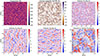 |
Fig. 1. Temperature, vertical magnetic field, and the three components of the velocity at log τ500 = 0 for the first considered timestep of the simulation. The black square in the upper-right panel marks the region shown in the lower-right panel. Arrows in the lower-right panel indicate horizontal velocities. |
2.3. Synthetic spectra and degradation
To create synthetic SUNRISE/TuMag observations, we calculated the emergent intensity of each pixel in the direction θ = 0 (disk center) for a range of wavelengths containing the line of neutral iron at 525.02 nm and the line of neutral magnesium at 517.2 nm (hereafter Fe I 525.0 nm and Mg I b2). The Fe I line is a photospheric spectral line with a large Landé factor (g = 3), which makes it a prime candidate for studies of photospheric magnetism. The Mg I line is a strong line with moderate sensitivity to the magnetic field (g = 1.75), which probes the photosphere and the temperature minimum. The choice of these lines was motivated by the observations performed with the TuMag instrument (del Toro Iniesta et al. 2025) at the SUNRISE (Solanki et al. 2010; Barthol et al. 2011) balloon-borne telescope, which completed its third successful flight in July 2024 (Korpi-Lagg et al. 2025).
For synthesis, we used spectropolarimetric non-local thermodynamic equilibrium (NLTE) analytically powered inversion (SNAPI; Milić & van Noort 2018), a 1D radiative transfer and inversion code that synthesizes a large number of spectra using message passing interface (MPI) parallelization. The code accounts for continuum and spectral line opacity, polarization due to the Zeeman effect, and NLTE effects in the Mg I b2 line. It accurately reproduces the observed shape of the Mg I b2 line (Vukadinović et al. 2022). Neutral iron is overionized in the solar photosphere due to UV radiation, and rigorous modeling would require an NLTE approach (Smitha et al. 2020). Such a calculation would be prohibitively expensive for the entire time series. Furthermore, because our study is primarily methodological, highly realistic, and precise modeling is beyond the scope of this paper.
The spectra were synthesized using every second pixel along x and y, increasing the spatial step to 32 km and making it comparable to the TuMag pixel scale (28 km; del Toro Iniesta et al. 2025). The spectra of the two lines were synthesized with 1 pm sampling, using 121 wavelengths for the Fe I 525.0 nm line and 501 wavelengths for the Mg I b2 line. The spectra were synthesized for all 31 time steps. The total number of resulting polarized spectra is therefore 768 × 768 × 31 ≈ 18 × 106. We synthesized two neutral iron lines around 525.0 nm, but only considered the more magnetically sensitive one, 3d64s2 → 3d6(5D)4s4p(3P0), with the central wavelength of 525.0208 nm. Figure 2 shows the synthetic intensity in the continuum, nominal cores of the two lines, and the circular polarization in the wings of the two lines. The map of the circular polarization in the Mg I b2 line was obtained by averaging Stokes V over a 50 mÅ interval, centered at the wavelength point 70 mÅ to the blue of the nominal line core. The map of the circular polarization in the Fe I 525.0 nm line was obtained similarly, but centered at the wavelength point 50 mÅ to the blue of the nominal line core. Section 4 presents the methods used to extract relevant physical quantities from these synthetic observations.
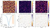 |
Fig. 2. Synthetic observables calculated for the first snapshot in the series. Top left: Continuum image at 517.2 nm. Top middle: Nominal line core of the Mg I b2 line. Top right: Nominal line core of Fe I 525.0 nm line. Bottom left: Spatially averaged spectra of the considered spectral lines, Fe I lines are shifted for clarity. Bottom middle: Circular polarization in the wing of the Mg I line. Bottom right: Circular polarization in the wing of the Fe I line. The upper-row panels are shown in units of the mean quiet-Sun continuum. |
3. Results
3.1. Tracking continuum intensity and magnetic field
To test the applicability of the FLCT technique for inferring horizontal velocities, we first applied it to the continuum intensity maps at λ = 500 nm, which are the output of the simulation, and to magnetograms, i.e., maps of the vertical component of the magnetic field vector at constant-τ500 corrugated surfaces, calculated using the MURaM code. We applied FLCT to the entire one-hour time series, which yielded a map of horizontal velocities for each pair of consecutive intensitygrams and magnetograms. We then compared the obtained velocities with horizontal velocities from the simulation (calculated as the average between two consecutive snapshots) at constant-τ500 surfaces. Direct comparison of these quantities yields relatively poor results (e.g. Verma et al. 2013; Tremblay et al. 2018). This occurs because the apodizing window used in FLCT automatically imposes a minimal spatial scale at which we can probe horizontal flows. Therefore, to compare the inferred and original velocities, the latter need to be convolved with a Gaussian filter that corresponds to the apodizing window used by FLCT. As shown by Verma et al. (2013) and Tremblay et al. (2018), the best agreement between the inferred and original velocities is achieved when both are averaged over a time interval that is much longer than the cadence of the analyzed images. For this dataset, we find that the best agreement occurs when both the inferred and original velocities are averaged over 15 minutes. Thus, each 15-minute interval yielded a single map of horizontal velocities, which was then compared to a single map of spatially convolved and temporally averaged simulated velocities. All comparisons in this and the following subsections are based on snapshots from the first 15 minutes of the simulated atmosphere. For the analysis of the synthetic spectra, we focused on the same 15-minute interval, sampled at a cadence of 30s cadence, corresponding to 31 cubes in total. For comparison, Verma et al. (2013) averaged over 15, 30, 60, 90, and 120-minute intervals. This time averaging step implies that, when applying FLCT, a compromise must be made between spatial and temporal resolution. This is a known limitation of FLCT techniques, which can be mitigated using recent machine learning-based tracking approaches (Asensio Ramos et al. 2017). Hereafter, we refer to the temporally averaged velocity inferred by FLCT as vf = (vx, vy)f, with the subindex f indicating that vf was obtained using FLCT from images of the quantity in parentheses. The temporally averaged and spatially filtered velocity from the simulation is denoted as vo = (vx, vy)o.
Figure 3 shows the comparison between the x component of vf, inferred by tracking the continuum intensity, and the x component of vo, for two different sizes of the apodizing windows: 600 km and 300 km. Figure 4 presents the same comparison for FLCT applied to Bz maps at log τ500 = 0 (i.e., the base of the photosphere). Because our motivation is the interpretation of high-resolution observations (while Verma et al. 2013, have tested apodizing windows in range 400−1800 km with a step of 200 km in order to benchmark the limitations of FLCT), we did not test apodizing windows larger than 600 km. Apodizing windows significantly below 300 km did not yield satisfactory agreement with the simulated velocities. This occurs because the assumptions of FLCT and the time averaging used in the comparison procedure do not resolve plasma motion on scales significantly below the spatial scales of the granules (as reported by Verma et al. 2013, for atmospheres simulated using CO5BOLD).
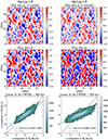 |
Fig. 3. Comparison between the x component of the horizontal velocity retrieved by FLCT applied to intensity maps and the simulated velocity at log τ500 = 0. Color maps indicate the magnitude of velocity. Bottom row: Scatter plot showing the least-squares fit between vo and vf. Results are shown for two different sizes of apodizing windows: left, 600 km; right, 300 km. |
Similar to previous studies, we find that, after spatial convolution and temporal averaging, the inferred and original velocities show excellent correlation (exceeding 0.9 for both x and y components and for both apodizing-window sizes), whether derived from intensity or Bz (see Table 1). However, FLCT underestimates the plasma velocity. For the apodizing window of 600 km, the inferred velocity is approximately three-fourths of the original value (see the bottom-left panels of Fig. 3), while for the 300 km window, it decreases to two-fifths (see the bottom-right panels of Fig. 3). Although this effect has been reported previously (see Verma et al. 2013), its origin is not fully understood. End-to-end studies of this kind can help calibrate this relationship and enable a more accurate interpretation of FCLT results applied to real-life observations.
Pearson’s correlation coefficients between simulated velocities and FLCT-derived velocities at the base of the photosphere.
The continuum intensity carries information from the iso-optical-depth surface at log τ500 = 0, corresponding to the base of the photosphere. To track the horizontal velocity at higher layers of the atmosphere, we need to identify the observables that probe these layers. In principle, spectroscopic or spectropolarimetric imaging (Iglesias & Feller 2019) in strong spectral lines enables the inference of physical parameters, such as temperature and magnetic field, at multiple atmospheric layers using spectropolarimetric inversion techniques (del Toro Iniesta & Ruiz Cobo 2016; de la Cruz Rodríguez & van Noort 2017). An important caveat is that spectroscopic and spectropolarimetric observations carry depth information on the optical depth scale. Thus, horizontal information inferred at a given optical depth corresponds to a corrugated surface in geometrical space. Accurate conversion from optical depth to geometrical height therefore requires additional physical constraints (e.g., Borrero et al. 2019, 2024).
3.2. Tracking temperature and magnetic field at multiple optical depths
To verify whether spectral line observation can probe horizontal velocities at multiple heights, we applied FLCT to the temperature and Bz at four layers above the base of the photosphere, log τ500 = { − 1, −2, −3, −4}, taken directly from the simulation. We then compared the results with the corresponding velocities in the simulation. Temperature was chosen as the tracking parameter because it is the closest possible quantity to intensity in a spectral line, formed at a specific depth, while Bz was chosen because polarization in different spectral lines is sensitive to the magnetic field at different depths. Tracking these two parameters provides a reference for what can be expected when tracking multi-depth physical quantities inferred from observations.
Figures 5 and 6 compare vf, inferred by tracking temperature and Bz, with vo at log τ500 = −1 and log τ500 = −3, for apodizing windows of 600 and 300 km. We chose a cadence of 30 s to match that of synthetic spectropolarimetric observations. Table 2 lists the Pearson correlation coefficients for all four optical depths and both velocity components. For temperature, the correlation clearly decreases with height. It drops from r ≈ 0.72 at log τ500 = −1 to r ≈ 0 at log τ500 = −3 and higher. By contrast, Bz is a suitable tracking parameter, as FLCT-inferred velocities exhibit a relatively high correlation with the original velocities at all optical depths analyzed. Closer inspection confirms that, structurally, the FLCT velocities derived from Bz closely match the original velocities, unlike in the case of temperature. The highest layer considered, at log τ500 = −4, may be affected by the choice of the upper boundary of the computational box. Comparison with similar MURaM simulations, which include much higher atmospheric layers (chromosphere and corona), reveal only small differences at log τ500 = −4, prompting us to retain this layer in our analysis.
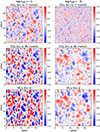 |
Fig. 5. Comparison between the x component of the horizontal velocity retrieved by FLCT using FWHM = 600 km, applied to temperature (top panel), and Bz (middle panel), and the simulated velocity (bottom panel) at log τ500 = { − 1, −3}. |
The stark difference between horizontal velocities obtained by tracking T and Bz arises because temperature is related to internal energy and experiences strong contributions from radiation transport, making its behavior far from advective. For Bz, we suppose that the changes are largely due to advection governed by the induction Equation (1), providing more robust features for tracking. Therefore, we conclude that FLCT-inferred velocities obtained from Bz serve as an excellent reference for expected results when applying FLCT to Stokes parameters in a spectral line. The following section examines tracking on Bz inferred from synthetic TuMag observations.
4. Application to synthetic polarized spectra
The previous section demonstrated that applying FLCT to Bz magnetograms extracted from simulation data yields a reliable inference of horizontal velocities for atmospheric layers from log τ500 = 0 to log τ500 = −4 (see Figs. 5 and 6, and Table 2). Next, we applied FLCT to the magnetograms obtained from the synthetic TuMag observations described in Sect. 2.3. By tracking the magnetograms obtained from the Fe I 525.0 nm and Mg I b2 lines, we aimed to track the horizontal velocity at the atmospheric heights probed by these two lines.
Pearson’s correlation coefficients between simulated velocities and FLCT velocities at the mid-photosphere and temperature minimum.
4.1. Inference of Bz
To infer Bz from the Stokes spectra of the Fe I 525.0 line, we used pyMilne, an efficient, parallel, spatially coupled Milne-Eddington inversion code (de la Cruz Rodríguez 2019). The Milne-Eddington approximation assumes a linear variation of the source function with optical depth, while the magnetic field and LOS velocity remain constant with depth. We applied pyMilne to each individual synthetic Stokes cube I(x, y, λ), where I denotes the Stokes vector, I = (I, Q, U, V)T. Each inversion yields a vector magnetogram B(x, y) for a given time step. It is important to adopt a so-called “formation height” for the line, to ascribe this inferred magnetic field to a specific atmospheric layer. To this end, we compared the inferred Bz to the original Bz at different iso-τ500 surfaces (by calculating the cross-correlation between the two, following, e.g. Vukadinović et al. 2022). We find the best agreement for log τ500 = −1, which is consistent with the typical formation heights of moderately strong photospheric lines (see, e.g., Borrero et al. 2014).
The Mg I b2 line is significantly stronger than Fe I 525.0 nm, which makes the Milne-Eddington approximation invalid (but see Dorantes-Monteagudo et al. 2022). We therefore used the weak-field approximation (WFA) to infer the longitudinal field, which coincides with Bz, under the disk-center assumption and in the absence of magnetic substructures below the pixel scale. The weak-field approximation assumes that the magnetic field is constant with height and that the Zeeman splitting it produces is much smaller than other sources of line broadening. This leads to the following relationship (e.g. Landi Degl’Innocenti & Landolfi 2004):
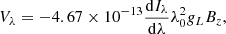 (4)
(4)
where the wavelengths are in Å, magnetic field is in G, and gL is the effective Landé factor of the line, in this case gL = 1.75. Given the large width of the Mg I line, the weak-field approximation is valid and probes depths around log τ500 = −3.3 (Vukadinović et al. 2022). We confirmed this by applying the weak-field approximation to the core of the Mg I line (0.2 Å around the intensity minimum) and comparing the inferred magnetic field with the original one in the simulation, again using cross-correlation. The best agreement occurs between log τ500 = −3 and log τ500 = −4.
Therefore, the two spectral lines probe different atmospheric layers: the mid-photosphere for Fe I 525.0 nm and the upper-photosphere or temperature-minimum region for Mg I b2. This is also evident in Fig. 2, where the Stokes V map in the Mg I line shows significantly less structure and more diffuse circular-polarization signals.
4.2. Tracking synthetic magnetograms
We applied FLCT to the synthetic magnetograms obtained from the two spectral lines to infer vf and compared it with vo at various optical depths. The synthetic spectra and magnetograms have different spatial sampling compared to the original simulation (32 km compared to 16 km). Figures 7 and 8 show the agreement between the inferred and the original velocities for two specific heights: log τ500 = −1 for the Fe line and log τ500 = −3 for the Mg line. Fig. 9 summarizes the comparison between the inferred and the original velocities. The vf inferred from the Fe I 525.0 nm line shows good agreement with vo(log τ500 = −1) and vo(log τ500 = −2), but the correlation decreases rapidly toward the higher layers. This behavior is consistent with our estimate of the depth where the Fe I line probes the magnetic field. The velocities inferred from the Mg I b2 line magnetograms agree best with vo(log τ500 = −3) and vo(log τ500 = −4), thereby probing regions near the temperature minimum and agreeing closely with the estimates of Vukadinović et al. (2022). Our results suggest that these two lines complement each other effectively in covering the whole vertical extent from the base of the photosphere (continuum) through the mid-photosphere (Fe I line) up to the temperature-minimum region (Mg I line).
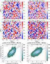 |
Fig. 7. Comparison between the x component of the horizontal velocity retrieved by FLCT applied to the synthetic magnetogram inferred from the Fe I line and the simulated velocity at log τ500 = −1. |
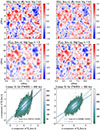 |
Fig. 8. Same as Fig. 7, but showing the synthetic magnetograms inferred from the Mg I line compared with the simulated velocity at log τ500 = −3. |
 |
Fig. 9. Pearson correlation coefficients between simulation velocities and velocities recovered by FLCT from Bz inferred either from Milne-Eddington inversions of the Fe I 525.0 nm line or from Bz inferred using the WFA approximation with the Mg I b2 line at log τ500 = { − 1, −2, −3, −4}, respectively. Correlations are shown only for filtered simulation velocities. |
The lower panels of Figs. 7 and 8 show that velocities inferred by tracking the synthetic magnetograms are also underestimated. This underestimation is larger for a smaller apodizing window, as already shown in Figs. 3 and 4. Furthermore, tracking synthetic magnetograms in the Mg I b2 line yields velocity amplitudes closer to the simulated values than those obtained from the Fe I line. This likely occurs because this line traces velocities higher in the atmosphere, where the flows are more diffuse and less spatially structured. Consequently, the FLCT algorithm can capture the properties of the flow more accurately.
For the spectral lines considered, applying tracking to the synthetic magnetograms yields somewhat poorer agreement than direct tracking of the magnetic fields at fixed optical depths (see Sect. 3.2). This outcome is not unexpected. The magnetic field in the solar atmosphere is height-dependent, and thus both the Milne-Eddington and WFA inversions introduce noticeable discrepancies and systematic errors. Depth-dependent magnetic field diagnostics using a more sophisticated inversion code could yield improvement, but at a significant computational cost, particularly due to the NLTE treatment of the Mg I b2 line (see the recent results of Siu-Tapia et al. 2025a,b).
4.3. Velocity divergence inferred from synthetic magnetograms
To further assess the reliability of horizontal velocity diagnostics using these spectral lines, we compared the divergence calculated from vf, inferred from synthetic magnetograms of the Fe I and Mg I spectral lines, with the value calculated from vo. In this context, the horizontal divergence is defined as
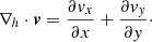 (5)
(5)
For instance, granules are expected to exhibit positive divergence, whereas intergranular lanes are dominated by negative divergence, corresponding to regions where flows converge.
The agreement is significantly poorer than for the individual comparison of the vx and vy components. For the magnetograms inferred from the Fe I line, the correlation coefficient is 0.29 for a 600 km FWHM and 0.20 for a 300 km FWHM. The agreement is even poorer for the Mg I b2 line, with correlation coefficients of 0.23 and 0.11 for the two apodizing windows, respectively. The poor estimation of divergences may stem from the fact that FLCT estimates velocities in neighboring pixels independently and does not incorporate spatial variations in the flow structure when estimating each pixel’s flow (cf. the DAVE, which is short for differential affine velocity estimator, method described by Schuck 2006). Consequently, no correlation is enforced between the neighboring pixel velocities. However, based on the nature of measurement uncertainties, the numerical differentiation used to compute the flow divergence also contributes to the discrepancy, as the uncertainty in the estimated velocity differences exceeds that of the individual velocity estimates. Consequently, we expect the derivatives of the estimated flows to be noisier than the flows themselves. Another source of disagreement arises because the simplified inversion methods effectively probe different depths at different pixels, which results in a different corrugation of inferred magnetic field maps between the original iso-τ500 slices and the obtained synthetic magnetograms.
To improve the agreement, we smoothed both the original and inferred divergence maps with a Gaussian filter of σ = 200 km, thereby further reducing the effective spatial resolution. This smoothing significantly improved the correlation coefficients to ≈0.6 for the Fe I magnetograms and ≈0.45 for the Mg I magnetograms (see Table 3). The comparison between the divergence inferred from the Fe I line and that derived from vo at log τ500 = −1 is presented in Fig. 10, while Fig. 11 shows the same comparison, but for the Mg I line and vo at log τ500 = −3. The pronounced difference between the ability of FLCT to reproduce horizontal velocities and their divergence indicates the presence of systematic discrepancies in the FLCT inference of horizontal velocities, as previously reported by Gibson et al. (2004) and Rempel et al. (2022). This limitation of the FLCT technique is expected to be improved by recently developed machine learning techniques (e.g. Asensio Ramos et al. 2017; Lennard et al. 2025).
Pearson correlation coefficient for divergence of FLCT and simulated velocities.
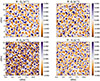 |
Fig. 10. Comparison between velocity divergence calculated using vo (left panels) at log τ500 = −1 and vf inferred from the Fe I line (right panels). Top: Results with an apodizing window of 600 km. Bottom: Results with an apodizing window of 300 km. |
5. Conclusions
We have studied the diagnostic potential of the FLCT flow-tracking technique to probe horizontal plasma flows at multiple heights in the lower solar atmosphere. First, we applied FCLT to a time series of intensitygrams, magnetograms, and temperature maps at constant optical depth surfaces ranging from log τ500 = 0 to log τ500 = −4, directly obtained from the simulation. After spatial filtering and temporal averaging (which is a standard procedure for velocities obtained with optical flow methods), we conclude that tracking LOS magnetograms yields satisfactory agreement with the original velocities across all considered optical depths. In contrast, tracking the temperature is unreliable for atmospheric layers above log τ500 = −1.
Next, we tracked synthetic magnetograms obtained through a simple but robust inversion of synthetic spectropolarimetric observables in two spectral lines: Fe I 525.0 nm and Mg I b2. These two lines probe the low-to-mid photosphere and the upper-photosphere or temperature-minimum regions, respectively. We synthesized the polarized spectra of the two lines using the SNAPI code (Milić & van Noort 2018) and then obtained synthetic magnetograms using the Milne-Eddington inversion code pyMilne (de la Cruz Rodríguez 2019) for the Fe I line and the weak-field approximation for the Mg I line. The inferred velocities agree well with the suitably filtered original ones, achieving correlation coefficients of r = 0.65 − 0.7. This result holds for both apodizing windows considered: 300 km and 600 km. The vertical magnetic field inferred from the Fe I 525.0 nm line accurately tracks horizontal velocities between log τ500 = −1 and log τ500 = −2, whereas the field inferred from the Mg I b2 line tracks the velocities in the higher regions, from log τ500 = −3 to log τ500 = −4. Therefore, fast-cadence imaging spectropolarimetry in these two spectral lines enables a robust inference of the horizontal velocities from the base of the photosphere to the temperature minimum. The important advantage of using spectral lines to track plasma flows is the potential to infer the vertical velocity or its vertical gradient (e.g., de la Cruz Rodríguez & van Noort 2017). However, the FLCT technique performs significantly worse when calculating the horizontal divergence of the velocity, yielding correlation coefficients of 0.6 or less.
These findings are especially relevant for the observations collected by the SUNRISE III/TuMag (del Toro Iniesta et al. 2025), the newly upgraded CRISP (Scharmer et al. 2008), and the upcoming VTF (Schmidt et al. 2016) instruments. The robust and simple magnetic field inference proposed here should be suitable for the relatively coarse wavelength sampling offered by these Fabry-Perot-based spectropolarimeters. The application to data from integral field units (IFUs) such as MiHI (van Noort et al. 2022) is more complex due to their spectral resolution, which may require more comprehensive inversion approaches. The limited range of spatial scales probed by FLCT represents a significant limitation of this method. Our results exhibit good agreement for apodizing windows of 600 km and 300 km, which are well above the diffraction limit of the instruments considered (≈80 km for SST and SUNRISE, and ≈20 km for DKIST, at visible wavelengths).
Inference of horizontal velocities from high-resolution observations requires further development and extensions of FLCT techniques or the application of recently developed AI-based methods, such as DeepVel (Asensio Ramos et al. 2017). Given that DeepVel can, in principle, infer horizontal velocities at multiple heights, training and applying it to spectral line data is expected to significantly improve its performance. Finally, the development of techniques that couple spectropolarimetric diagnostics with MHD equations (Borrero et al. 2019, 2024), possibly combined with physically informed neural networks (Jarolim et al. 2023; Tremblay et al. 2023), is expected to provide the most robust and physically meaningful information on plasma conditions, including horizontal velocities.
Acknowledgments
We gratefully acknowledge the ISSI team devoted to tracking flows in the solar atmosphere. We are indebted to an anonymous referee for their careful reading of the paper and insightful comments, which significantly improved the clarity and presentation of this work. TK and IM acknowledge the financial support from the Serbian Ministry of Science and Technology through the grants 451-03-136/2025-03/200104 and 451-03-136/2025-03/200002. M.D.K. acknowledges support by NASA ECIP award 80NSSC19K0910, NASA HSR-80NSSC23K0092 and NSF CAREER award SPVKK1RC2MZ3. AAR acknowledges support from the Agencia Estatal de Investigación del Ministerio de Ciencia, Innovación y Universidades (MCIU/AEI) and the European Regional Development Fund (ERDF) through project PID2022-136563NB-I0. BTW gratefully acknowledges support from NASA HSR-80NSSC23K0092. This material is based upon work supported by the NSF National Center for Atmospheric Research, which is a major facility sponsored by the U.S. National Science Foundation under Cooperative Agreement No. 1852977. We would like to acknowledge high-performance computing support from the Derecho system (doi:10.5065/qx9a-pg09) provided by the NSF National Center for Atmospheric Research (NCAR), sponsored by the National Science Foundation. This research has made use of NASA’s Astrophysics Data System.
References
- Afanasyev, A. N., Kazachenko, M. D., Fan, Y., Fisher, G. H., & Tremblay, B. 2021, ApJ, 919, 7 [NASA ADS] [CrossRef] [Google Scholar]
- Arregui, I. 2015, Philos. Trans. R. Soc. A, 373, 20140261 [Google Scholar]
- Asensio Ramos, A., Requerey, I. S., & Vitas, N. 2017, A&A, 604, A11 [NASA ADS] [CrossRef] [EDP Sciences] [Google Scholar]
- Barthol, P., Gandorfer, A., Solanki, S. K., et al. 2011, Sol. Phys., 268, 1 [Google Scholar]
- Borrero, J. M., Lites, B. W., Lagg, A., Rezaei, R., & Rempel, M. 2014, A&A, 572, A54 [NASA ADS] [CrossRef] [EDP Sciences] [Google Scholar]
- Borrero, J. M., Pastor Yabar, A., Rempel, M., & Ruiz Cobo, B. 2019, A&A, 632, A111 [NASA ADS] [CrossRef] [EDP Sciences] [Google Scholar]
- Borrero, J. M., Pastor Yabar, A., & Ruiz Cobo, B. 2024, A&A, 687, A155 [NASA ADS] [CrossRef] [EDP Sciences] [Google Scholar]
- Chae, J., & Sakurai, T. 2008, ApJ, 689, 593 [NASA ADS] [CrossRef] [Google Scholar]
- Charbonneau, P. 2010, Living Rev. Sol. Phys., 7, 3 [NASA ADS] [CrossRef] [Google Scholar]
- Danilovic, S., Rempel, M., van Noort, M., & Cameron, R. 2016, A&A, 594, A103 [NASA ADS] [CrossRef] [EDP Sciences] [Google Scholar]
- de la Cruz Rodríguez, J. 2019, A&A, 631, A153 [NASA ADS] [CrossRef] [EDP Sciences] [Google Scholar]
- de la Cruz Rodríguez, J., & van Noort, M. 2017, Space Sci. Rev., 210, 109 [Google Scholar]
- del Toro Iniesta, J. C., & Ruiz Cobo, B. 2016, Living Rev. Sol. Phys., 13, 4 [Google Scholar]
- del Toro Iniesta, J. C., Orozco Suárez, D., Álvarez-Herrero, A., et al. 2025, ArXiv e-prints [arXiv:2502.08268] [Google Scholar]
- Demoulin, P., & Berger, M. 2003, Sol. Phys., 215, 203 [CrossRef] [Google Scholar]
- Dorantes-Monteagudo, A. J., Siu-Tapia, A. L., Quintero-Noda, C., & Orozco Suárez, D. 2022, A&A, 659, A156 [NASA ADS] [CrossRef] [EDP Sciences] [Google Scholar]
- Fisher, G. H., & Welsch, B. T. 2008, ASP Conf. Ser., 383, 373 [NASA ADS] [Google Scholar]
- Fisher, G. H., Kazachenko, M. D., Welsch, B. T., et al. 2020, ApJS, 248, 2 [NASA ADS] [CrossRef] [Google Scholar]
- Gibson, S. E., Fan, Y., Mandrini, C., Fisher, G., & Demoulin, P. 2004, ApJ, 617, 600 [Google Scholar]
- Iglesias, F. A., & Feller, A. 2019, Opt. Eng., 58, 082417 [Google Scholar]
- Jarolim, R., Thalmann, J. K., Veronig, A. M., & Podladchikova, T. 2023, Nat. Astron., 7, 1171 [NASA ADS] [CrossRef] [Google Scholar]
- Kazachenko, M. D., Fisher, G. H., & Welsch, B. T. 2014, ApJ, 795, 17 [NASA ADS] [CrossRef] [Google Scholar]
- Korpi-Lagg, A., Gandorfer, A., Solanki, S. K., et al. 2025, Sol. Phys., 300, 75 [Google Scholar]
- Landi Degl’Innocenti, E., & Landolfi, M. 2004, Polarization in Spectral Lines (Dordrecht: Kluwer Academic Publishers) [Google Scholar]
- Leenaarts, J., van Noort, M., de la Cruz Rodríguez, J., et al. 2025, A&A, 696, A3 [NASA ADS] [CrossRef] [EDP Sciences] [Google Scholar]
- Lennard, M. G., Silva, S. S. A., Tremblay, B., et al. 2025, MNRAS, 539, 2498 [Google Scholar]
- Li, Z. F., Cheng, X., Ding, M. D., et al. 2021, ApJ, 915, 124 [Google Scholar]
- Liu, J., Nelson, C. J., Snow, B., Wang, Y., & Erdélyi, R. 2019, Nat. Commun., 10, 3504 [Google Scholar]
- Löptien, B., Birch, A. C., Duvall, T. L., Gizon, L., & Schou, J. 2016, A&A, 590, A130 [Google Scholar]
- Lumme, E., Kazachenko, M. D., Fisher, G. H., et al. 2019, Sol. Phys., 294, 84 [NASA ADS] [CrossRef] [Google Scholar]
- Milić, I., & van Noort, M. 2018, A&A, 617, A24 [Google Scholar]
- Nordlund, A. 1982, A&A, 107, 1 [Google Scholar]
- Nordlund, Å., Stein, R. F., & Asplund, M. 2009, Living Rev. Sol. Phys., 6, 2 [Google Scholar]
- November, L. J., & Simon, G. W. 1988, ApJ, 333, 427 [Google Scholar]
- Rempel, M. 2014, ApJ, 789, 132 [Google Scholar]
- Rempel, E. L., Chertovskih, R., Davletshina, K. R., et al. 2022, ApJ, 933, 2 [NASA ADS] [CrossRef] [Google Scholar]
- Rieutord, M., Roudier, T., Ludwig, H. G., Nordlund, Å., & Stein, R. 2001, A&A, 377, L14 [NASA ADS] [CrossRef] [EDP Sciences] [Google Scholar]
- Scharmer, G. B., Narayan, G., Hillberg, T., et al. 2008, ApJ, 689, L69 [Google Scholar]
- Schmidt, W., Schubert, M., Ellwarth, M., et al. 2016, SPIE Conf. Ser., 9908, 99084N [NASA ADS] [Google Scholar]
- Schou, J., Scherrer, P. H., Bush, R. I., et al. 2012, Sol. Phys., 275, 229 [Google Scholar]
- Schuck, P. W. 2006, ApJ, 646, 1358 [Google Scholar]
- Siu-Tapia, A. L., Bellot Rubio, L. R., & Orozco Suárez, D. 2025a, A&A, 696, A105 [NASA ADS] [CrossRef] [EDP Sciences] [Google Scholar]
- Siu-Tapia, A. L., Bellot Rubio, L. R., Orozco Suárez, D., & Gafeira, R. 2025b, A&A, 696, A106 [NASA ADS] [CrossRef] [EDP Sciences] [Google Scholar]
- Skirvin, S. J., Fedun, V., Goossens, M., Silva, S. S. A., & Verth, G. 2024, ApJ, 975, 176 [Google Scholar]
- Smitha, H. N., Holzreuter, R., van Noort, M., & Solanki, S. K. 2020, A&A, 633, A157 [NASA ADS] [CrossRef] [EDP Sciences] [Google Scholar]
- Solanki, S. K., Barthol, P., Danilovic, S., et al. 2010, ApJ, 723, L127 [NASA ADS] [CrossRef] [Google Scholar]
- Stein, R. F. 2012, Living Rev. Sol. Phys., 9, 4 [Google Scholar]
- Tilipman, D., Kazachenko, M., Tremblay, B., et al. 2023, ApJ, 956, 83 [Google Scholar]
- Tremblay, B., Roudier, T., Rieutord, M., & Vincent, A. 2018, Sol. Phys., 293, 57 [NASA ADS] [CrossRef] [Google Scholar]
- Tremblay, B., Jarolim, R., Rempel, M., et al. 2023, AAS/Solar Physics Division Meeting, 55, 202.01 [Google Scholar]
- van Noort, M., Bischoff, J., Kramer, A., Solanki, S. K., & Kiselman, D. 2022, A&A, 668, A149 [NASA ADS] [CrossRef] [EDP Sciences] [Google Scholar]
- Verma, M., Steffen, M., & Denker, C. 2013, A&A, 555, A136 [NASA ADS] [CrossRef] [EDP Sciences] [Google Scholar]
- Vögler, A., Shelyag, S., Schüssler, M., et al. 2005, A&A, 429, 335 [Google Scholar]
- Vukadinović, D., Milić, I., & Atanacković, O. 2022, A&A, 664, A182 [NASA ADS] [CrossRef] [EDP Sciences] [Google Scholar]
- Welsch, B. T. 2015, PASJ, 67, 18 [Google Scholar]
- Welsch, B. T., Fisher, G. H., Abbett, W. P., & Regnier, S. 2004, ApJ, 610, 1148 [NASA ADS] [CrossRef] [Google Scholar]
- Welsch, B. T., Abbett, W. P., De Rosa, M. L., et al. 2007, ApJ, 670, 1434 [NASA ADS] [CrossRef] [Google Scholar]
- Welsch, B. T., Kusano, K., Yamamoto, T. T., & Muglach, K. 2012, ApJ, 747, 130 [NASA ADS] [CrossRef] [Google Scholar]
All Tables
Pearson’s correlation coefficients between simulated velocities and FLCT-derived velocities at the base of the photosphere.
Pearson’s correlation coefficients between simulated velocities and FLCT velocities at the mid-photosphere and temperature minimum.
Pearson correlation coefficient for divergence of FLCT and simulated velocities.
All Figures
|
Fig. 1. Temperature, vertical magnetic field, and the three components of the velocity at log τ500 = 0 for the first considered timestep of the simulation. The black square in the upper-right panel marks the region shown in the lower-right panel. Arrows in the lower-right panel indicate horizontal velocities. |
| In the text | |
|
Fig. 2. Synthetic observables calculated for the first snapshot in the series. Top left: Continuum image at 517.2 nm. Top middle: Nominal line core of the Mg I b2 line. Top right: Nominal line core of Fe I 525.0 nm line. Bottom left: Spatially averaged spectra of the considered spectral lines, Fe I lines are shifted for clarity. Bottom middle: Circular polarization in the wing of the Mg I line. Bottom right: Circular polarization in the wing of the Fe I line. The upper-row panels are shown in units of the mean quiet-Sun continuum. |
| In the text | |
|
Fig. 3. Comparison between the x component of the horizontal velocity retrieved by FLCT applied to intensity maps and the simulated velocity at log τ500 = 0. Color maps indicate the magnitude of velocity. Bottom row: Scatter plot showing the least-squares fit between vo and vf. Results are shown for two different sizes of apodizing windows: left, 600 km; right, 300 km. |
| In the text | |
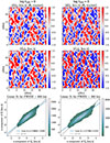 |
Fig. 4. Same as Fig. 3, but for FLCT applied to Bz at log τ500 = 0. |
| In the text | |
|
Fig. 5. Comparison between the x component of the horizontal velocity retrieved by FLCT using FWHM = 600 km, applied to temperature (top panel), and Bz (middle panel), and the simulated velocity (bottom panel) at log τ500 = { − 1, −3}. |
| In the text | |
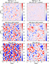 |
Fig. 6. Same as Fig. 5, except that FWHM = 300 km. |
| In the text | |
|
Fig. 7. Comparison between the x component of the horizontal velocity retrieved by FLCT applied to the synthetic magnetogram inferred from the Fe I line and the simulated velocity at log τ500 = −1. |
| In the text | |
|
Fig. 8. Same as Fig. 7, but showing the synthetic magnetograms inferred from the Mg I line compared with the simulated velocity at log τ500 = −3. |
| In the text | |
|
Fig. 9. Pearson correlation coefficients between simulation velocities and velocities recovered by FLCT from Bz inferred either from Milne-Eddington inversions of the Fe I 525.0 nm line or from Bz inferred using the WFA approximation with the Mg I b2 line at log τ500 = { − 1, −2, −3, −4}, respectively. Correlations are shown only for filtered simulation velocities. |
| In the text | |
|
Fig. 10. Comparison between velocity divergence calculated using vo (left panels) at log τ500 = −1 and vf inferred from the Fe I line (right panels). Top: Results with an apodizing window of 600 km. Bottom: Results with an apodizing window of 300 km. |
| In the text | |
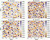 |
Fig. 11. Same as Fig. 10 but for the Mg I line and log τ500 = −3. |
| In the text | |
Current usage metrics show cumulative count of Article Views (full-text article views including HTML views, PDF and ePub downloads, according to the available data) and Abstracts Views on Vision4Press platform.
Data correspond to usage on the plateform after 2015. The current usage metrics is available 48-96 hours after online publication and is updated daily on week days.
Initial download of the metrics may take a while.