| Issue |
A&A
Volume 705, January 2026
|
|
|---|---|---|
| Article Number | A219 | |
| Number of page(s) | 16 | |
| Section | Extragalactic astronomy | |
| DOI | https://doi.org/10.1051/0004-6361/202556251 | |
| Published online | 20 January 2026 | |
J-PAS: A neural network approach to single stellar population characterisation
1
Instituto de Física de Cantabria Av. de los Castros 39005 Santander Cantabria, Spain
2
Centro de Estudios de Física del Cosmos de Aragón, Plaza de San Juan, 1 E-44001 Teruel, Spain
3
Unidad Asociada CEFCA-IAA, CEFCA, Unidad Asociada al CSIC por el IAA y el IFCA Plaza San Juan 1 44001 Teruel, Spain
4
Universidade de São Paulo, Instituto de Astronomia, Geofisica e Ciências Atmosféricas, Rua do Matão 1226 05508-090 São Paulo SP, Brazil
5
Instituto de Radioastronomía y Astrofísica, Universidad Nacional Autónoma de México, Morelia Michoacán 58089, Mexico
6
Instituto de Astrofísica de Andalucía (CSIC) PO Box 3004 18080 Granada, Spain
7
Tartu Observatory, University of Tartu Observatooriumi 1 Tõravere 61602, Estonia
8
Observatori Astronòmic de la Universitat de València, Ed. Instituts d’Investigació, Parc Científic. C/ Catedrático José Beltrán, n2 46980 Paterna Valencia, Spain
9
Departament d’Astronomia i Astrofísica, Universitat de València 46100 Burjassot, Spain
10
NSF NOIRLab Tucson AZ 85719, USA
11
Departamento de Astronomia, Instituto de Astronomia, Geofísica e Ciências Atmosféricas, Universidade de São Paulo São Paulo, Brazil
12
Observatório Nacional, Rua General José Cristino, 77 São Cristóvão 20921-400 Rio de Janeiro RJ, Brazil
13
Donostia International Physics Center (DIPC), Manuel Lardizabal Ibilbidea, 4 San Sebastián, Spain
14
Instituto de Astrofísica de Canarias C/ Vía Láctea s/n E-38205 La Laguna Tenerife, Spain
15
Universidad de La Laguna, Avda Francisco Sánchez E-38206 San Cristóbal de La Laguna Tenerife, Spain
16
Instruments4 4121 Pembury Place La Canada Flintridge CA 91011, USA
★ Corresponding author: This email address is being protected from spambots. You need JavaScript enabled to view it.
Received:
4
July
2025
Accepted:
10
November
2025
Abstract
J-PAS (Javalambre Physics of the Accelerating Universe Astrophysical Survey) will present a groundbreaking photometric survey covering 8500 deg2 of the visible sky from Javalambre, capturing data in 56 narrow-band filters. This survey promises to revolutionise galaxy evolution studies by observing ∼108 galaxies with low spectral resolution. A crucial aspect of this analysis involves predicting stellar population parameters from the observed galaxy photometry. In this study, we combined the exquisite J-PAS photometry with state-of-the-art single stellar population (SSP) libraries to accurately predict stellar age, metallicity, and dust attenuation with a neural network (NN) model. The NN was trained on synthetic J-PAS photometry from different SSP libraries (E-MILES, Charlot & Bruzual, and XSL) to enhance the robustness of our predictions against individual SSP model variations and limitations. To create mock samples with varying observed magnitudes, we added artificial noise in the form of random Gaussian variations within typical observational uncertainties in each band. Our results indicate that the NN was able to accurately estimate stellar parameters for SSP models without any evident degeneracies, surpassing a Bayesian SED-fitting method on the same test set. We obtained the median bias, scatter, and the percentage of outliers: μ= (0.01 dex, 0.00 dex, 0.00 mag), σNMAD= (0.23 dex, 0.29 dex, 0.04 mag), fo= (17%, 24%, 1%) at i ∼ 17 mag for the age, metallicity and dust attenuation, respectively. The accuracy of the predictions is highly dependent on the signal-to-noise ratio (S/N) of the photometry, achieving robust predictions up to i ∼ 20 mag.
Key words: galaxies: fundamental parameters / galaxies: photometry / galaxies: stellar content
© The Authors 2026
 Open Access article, published by EDP Sciences, under the terms of the Creative Commons Attribution License (https://creativecommons.org/licenses/by/4.0), which permits unrestricted use, distribution, and reproduction in any medium, provided the original work is properly cited.
This article is published in open access under the Subscribe to Open model. This email address is being protected from spambots. You need JavaScript enabled to view it. to support open access publication.
1. Introduction
The field of galaxy evolution is aimed at improving our understanding of how galaxy properties have changed across cosmic time and how these properties are related. The main attributes of galaxies include the morphology, the environment, and the stellar populations (i.e. the stars contained within them. The assembly histories of galaxies leave their imprint on the stellar populations and interstellar medium, which can be characterised by the total stellar mass, mean age of the stellar population, metallicity and dust content, among other parameters. Unveiling the stellar population of large numbers of galaxies is fundamental to gaining knowledge of the processes that have given rise to the great variety of galaxies that we see in the Universe.
Single stellar population (SSP) models combine spectral stellar libraries with isochrones to predict the time-evolution of the light emitted by a galaxy with a given initial mass function (IMF) and metallicity [M/H]. By comparing these theoretical models with the observations, the stellar properties of the galaxies can be estimated. This can be done through full-spectral fitting (e.g. Cid Fernandes et al. 2005; Cappellari et al. 2011) or spectral index measurements (e.g. Trager et al. 2000; Serven et al. 2005; Eftekhari et al. 2021) when spectroscopic observations or narrow-band photometry are available (e.g. Hernán-Caballero et al. 2013, 2014; Domínguez Sánchez et al. 2016) or by means of a spectral energy distribution (SED) fitting (e.g. Boquien et al. 2019; Díaz-García et al. 2015; Robotham et al. 2020) for photometric observations.
The improved spectral resolution of spectroscopy enables more accurate measurements of the stellar populations, but spectroscopic observations are very time consuming and often require pre-selected targets, biasing the analysis to relatively bright objects and smaller samples. On the other hand, photometric surveys are only limited by their depth and usually cover large areas of the sky, but their insufficient spectral resolution complicates the estimation of stellar populations, sharpening the well-known age-metallicity-attenuation degeneracies (e.g. Díaz-García et al. 2015). In this work, we take advantage of the Javalambre Physics of the Accelerating Universe Astrophysical Survey (J-PAS), providing photometry in 56 narrow bands (plus the i-band for detection) that provides pseudo-spectra with a resolution R ∼ 60 and it is almost complete up to i < 22.0 mag. J-PAS will observe roughly 1/5 of the sky, providing extremely valuable information for hundreds of millions of galaxies (Benitez et al. 2014; Bonoli et al. 2021). Extracting stellar population parameters for these wealthy dataset is a challenging and time-consuming task, but the reward is worth it, since the scientific applications of these estimates are innumerable.
While traditional SED-fitting codes have been widely utilised for this purpose, they often require a predefined set of templates for comparison, which can be computationally intensive. Moreover, a limited parameter space may fail to adequately represent the galaxy population. In recent years, there has been a surge in the application of machine learning algorithms, particularly neural networks (NNs) for various tasks in astronomy (e.g. Whitten et al. 2019; Galarza et al. 2022; Martínez-Solaeche et al. 2022; Wang et al. 2022; Martínez-Solaeche et al. 2023; del Pino et al. 2024; Gurung-López et al. 2022, 2025); particularly in image analysis (e.g. Domínguez Sánchez et al. 2018, 2019b; Walmsley et al. 2022; Domínguez Sánchez et al. 2023; Bom et al. 2024 to mention a few, see Huertas-Company & Lanusse 2023 for a complete review). However, their potential for predicting stellar populations of galaxies has remained barely unexplored (Liew-Cain et al. 2021; Woo et al. 2024; Wang et al. 2024; Iglesias-Navarro et al. 2024), offering considerable room for exploration.
In this work, we combine the high precision J-PAS photometry with cutting-edge SSP models (E-MILES, Charlot & Bruzual, XSL) to estimate stellar population parameters with NNs. We used synthetic photometry with realistic noise to train and test the NN models. In Sect. 2, we describe the SSP libraries and how the synthetic photometry was computed. In Sect. 3, we give details on the NN and training strategy. We show our results on the synthetic photometry in Sect. 4 and compare them with previous works and SED-fitting results in Sect. 5. In Sect. 6 we present the predictions for a sample of real local galaxies observed by the first J-PAS data release. Finally, Sect. 7 summarises our findings.
2. Data
In this section, we describe the SSP libraries used in this work. We also discuss how we generated the synthetic J-PAS photometry to train and test our NN for estimating SSP properties.
2.1. Single stellar population models
In this work, we use supervised learning to train a NN to predict SSP properties (age, metallicity, dust attenuation) from J-PAS photometry. To ensure a reliable ground truth, we used SSP synthesis models (for which these parameters are well known), instead of real galaxies, where the stellar populations have to be derived by other means (e.g. SED or spectral fitting), with their associated uncertainties and biases.
A SSP model is defined by a single age, metallicity, and IMF, while galaxies are composed by mixtures of populations. However, when we refer to the age of a stellar population, the concept can be ambiguous, as its definition varies across different studies. In SEDs and spectral fittings, the most commonly used definitions are mass-weighted or light-weighted ages, but other definitions can be adopted (see Sect. 3.3 in Gonçalves et al. 2020). These codes adopt either non-parametric, such as MUFFIT (Díaz-García et al. 2015), STARLIGHT (Cid Fernandes et al. 2011), PPXF (Cappellari & Emsellem 2004), or parametric star formation histories (SFHs), such as BAYSEAGAL (González Delgado et al. 2021), PROSPECT (Johnson et al. 2021), and CIGALE (Boquien et al. 2019). In the non-parametric case, mixtures of an arbitrary number of SSPs require strategies to explore the parameter space in search of the minima, as it is not feasible to forward model all possible combinations of SSPs. In the case of parametric codes, the parametric form of the SFH and age-metallicity relations need to be adopted a priori, which often introduces biases and results in less accurate inferred parameters (e.g. Leja et al. 2019). Flexible SFHs that are meant to come closer to the behaviour of the non-parametric descriptions are in development (e.g. Bellstedt et al. 2020). Nonetheless, it is important to note that the forward modelling of galaxy SEDs from all possible combinations requires dedicated work.
In our analysis, we have taken a simpler approach and approximated the galaxy SED to one SSP, as commonly adopted in classical stellar population works using spectral indices (e.g. Trager et al. 2000; Thomas et al. 2005; Vazdekis et al. 2010). For instantaneous SFHs, the SSP-equivalent, light-weighted and mass-weighted parameters are equivalent. For extended SFHs, the correlation between the parameters has been investigated in the literature (e.g. Serra & Trager 2007; Trager & Somerville 2009). By analysing a series of mock galaxies, these works show that SSP-equivalent and light-weighted ages are correlated, with the light-weighted ages falling in between the SSP-equivalent and the mass-weighted ages. The SSP-equivalent age mostly measures the most recent star formation and can be interpreted as a lower limit of the ages in the studied population. On the other hand, the SSP-equivalent metallicities depend mainly on the chemical composition of the old population and closely track the mass- and light-weighted metallicities. For the goals of this paper and to keep our discussion simple and clear, we believe that limiting our analysis to SSPs is justified. We discuss the estimates of our NN – trained on SSP – on composite stellar populations (CSP) in Appendix C.
We used three state-of-the-art SSP libraries, commonly used in the literature: E-MILES (Vazdekis et al. 2016), Charlot&Bruzual 2019 (Plat et al. 2019, CB19 hereafter), and the X-shooter Spectral Library (Verro et al. 2022a, XSL). By combining different SSP libraries in our training, we have aimed to make the model more robust against spectral resolution or any bias that may arise from the parameter space sampling of the SSP libraries. In addition, we note that after several tests, we found a better performance of the NN predictions when the three SSP libraries were combined together in the training. We summarise some important characteristics of each SSP library below. We refer to the corresponding references for a more detailed description.
2.1.1. E-MILES library
The UV-extended E-MILES stellar population synthesis models cover the spectral range 1680–50 000 Å at moderately high resolution. The space-based New Generation Stellar Library was used to compute spectra of single-age, single-metallicity stellar populations in the wavelength range from 1680 to 3540 Å, joined with those computed in the visible using MILES, and other empirical libraries for redder wavelengths. We used the isochrones Padova2000 and BaSTI (Girardi et al. 2000; Pietrinferni et al. 2004). The models span the metallicity range −2.32 ≤ [M/H] ≤ +0.4 and ages above 30 Myr (i.e. they do not include starburst and post-starburst populations) for a suite of initial mass function (IMF) types with varying slopes. In particular, in this work, we use the Chabrier (2003), Kroupa (2001) and Unimodal Γ = 1.3 IMFs. The original models have no dust attenuation. We have generated a new set of models by reddening each of the original models to different values1 using the law from Cardelli et al. (1989) with R = 3.1. The left panel of Fig. 1 shows the age-metallicity parameter space covered by the 26 622 E-MILES models used in this work compared to the parameter spaced covered by the three SP libraries combined together.
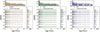 |
Fig. 1. Age-metallicity coverage of the three SSP synthesis models used in this work to train the NNs. The grey symbols (dots and histograms) show the combination of the three SSP libraries. In each panel, we show the individual libraries: E-MILES in orange (left panel), CB19 in green (middle panel), and XSL in blue (right panel). Note: Models with ages < 30 Myr are only included in the CB19 SSP library. |
2.1.2. Charlot & Bruzual 2019 library
The CB19 stellar population synthesis models cover the spectral range 5–80 000 Å at moderate-to-high spectral resolution using stellar fluxes from the literature, PARSEC isochrones and Chabrier (2003) IMF. The age-metallicity coverage of the 29 700 CB19 models used in this work is shown in the middle panel of Fig. 1, covering −2.23 ≤ [M/H] ≤ +0.54 and ages above 1.5 Myr, comprising the library that includes the youngest populations. As explained for the E-MILES, we generated a new set of models with different E(B-V) values.
2.1.3. XSL library
The XSL SSP models are based on the empirical X-shooter Spectral Library DR3 (Verro et al. 2022b), a moderate-to-high resolution, near-ultraviolet-to-near-infrared (NUV-NIR of 3500–24 800 Å, R∼ 10 000) spectral library, composed of 830 stellar spectra of 683 stars. The wavelength coverage and careful modelling of the RGB and AGB fluxes is optimised to bridge optical and NIR studies of intermediate-age and old stellar populations. The models span the metallicity range −2.2 < [Fe/H] < +0.25 and ages above 50 Myr (i.e. no starburst or post-starburst included), with PARSEC and Padova2000 isochrones and two IMF parametrisations (Salpeter 1955 and Kroupa 2001). We also generated a new set of models with different E(B-V) values for this library. The age-metallicity covered by the 9936 XSL models used in this work is shown in the right panel of Fig. 1.
Number of SSP models for the different libraries for the original and the mock samples.
2.2. J-PAS photometry
J-PAS is a wide-field cosmological survey performed with the 1.2 Gigapixel JPCam instrument of the 2.5 m JAST250 telescope at the Javalambre Observatory (Teruel, Spain). J-PAS observations, started in October 2023, will eventually cover ∼8500 deg2 of the northern sky (Benitez et al. 2014; Bonoli et al. 2021). Its unique set of 56 narrow bands (FWHM ∼ 140 Å) spanning the optical range from 3500 Å to 9300 Å allows excellent photometric redshift accuracy (σz= 0.003; Hernán-Caballero et al. 2021) and precise measurement of the stellar populations of galaxies (e.g. Benitez et al. 2014; Mejía-Narváez et al. 2017; González Delgado et al. 2021).
The synthetic J-PAS photometry is generated by convolving the SSP spectra (described in Section 2) with the official J-PAS filter transmission curves2. Dust attenuation is applied directly to the spectra before computing the photometry (see details in Section 2.1.1). Figure 2 gives examples of the synthetic photometry for a young and an old SSP with different metallicities and dust attenuation from the E-MILES library. Some of the spectral features are clearly visible in the synthetic fluxes (e.g. Mg and Na absorption). We note that the models are at rest-frame wavelength (z = 0) and have no noise. Since the objective of this project is to predict SP from observed galaxies, we needed to model and apply noise to the synthetic photometry to make the data more similar to real observations. In order to do so, we applied random Gaussian variations to the SSP fluxes, where the amplitude σ of the variations was derived as the average of the photometric error of the galaxies in mini-JPAS3, Δm4, as a function of AUTO magnitude in each band. Figure 3 shows these errors (in magnitude) for each band at different observed magnitudes. We generated the synthetic spectra of the mock observed magnitudes from i = 16.0–22.0 mag in 0.5 magnitude bins; thus, we multiplied the number of SSP models by 13. As an example, Fig. 3 illustrates one of these mock SSPs with different levels of noise (corresponding to different observed magnitudes). The number of SSP models from each library (original and with different levels of noise) are given in Table 1.
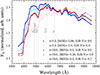 |
Fig. 2. Examples of synthetic J-PAS photometry from E-MILES SSP for a young (3 Gyr) and an old (10 Gyr) SSP with different metallicities and dust attenuation, as stated in the legend. Fluxes are normalised to the mean value of the flux for each SSP. Note: Subtle differences need to be distinguished for a proper characterisation of the SSPs (e.g. compare the red and purple lines). |
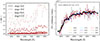 |
Fig. 3. Left: Average magnitude error of mini-JPAS galaxies for the 57 filters for different observed magnitudes (16, 18, 20, and 22 mag). Right: Synthetic J-PAS photometry obtained after applying random Gaussian variations consistent with the typical errors at different magnitudes. Colours represent different mock observed magnitudes. The thick dashed black line is the original SED. |
3. Neural network: Architecture and training strategy
We employed a simple neural network (NN) architecture to train our machine learning model, taking as our input a data vector of 57 dimensions with the J-PAS flux in each filter (in Fν, normalised by the median value of the flux of each SSP model). The labels correspond to the SP parameters (age5, [M/H] and E(B-V)). We explored two different NN configurations:
-
base NN: a hidden layer with 128 neurons, three hidden layers with 256 neurons each and a dense layer returning the output (172 289 free parameters);
-
SED NN6: a hidden layer with 128 neurons, six hidden layers with 300 neurons each and a dense layer returning the output (497 925 free parameters).
We found better results with the base NN configuration, despite its smaller number of free parameters. This suggests that a simpler model is suitable for the analysis presented in this work, while preventing any over-fitting. We trained over 100 epochs, using the mean square error (MSE) as loss function, ADAM optimiser, and learning rate lr = 0.002. Better results were obtained when using batchsize = 32 rather than 100 or 1000, even when combined with dropout. In particular, a small batch size significantly reduced over-fitting. The comparison is shown in Fig. A.1 in Appendix A. We trained three independent NNs (i.e. the output dimension is one), one for each of the parameters (age, metallicity, and attenuation). We found better results with this configuration, rather than training a single model with a three-dimensional (3D) output.
We randomly split our sample into training, validation, and test sub-samples with a 65/15/20 proportion, resulting in 551 253, 172 263, and 137 838 SSP models, respectively. The distributions of the input SSP parameters for each sub-set are shown in Fig. 4. The loss plots displaying the training behaviour are reported in Appendix B.
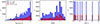 |
Fig. 4. Age (left panel), metallicity (middle panel) and dust attenuation (right panel) distribution for the training (blue), test (red), and validation (empty black) sub-samples. The sub-samples are randomly selected, showing no differences in their distributions. |
4. Results
In this section, we evaluate the NN model performance by comparing the input versus the predicted SSP parameters. In Fig. 5, we show the predicted versus the input ages for all galaxies up to magnitude i < 22 mag, as well as for galaxies with i = 16, 18, and 20. The agreement between the input and the predicted stellar age is excellent, with almost no average median bias (μ= 0.01 dex) and a small scatter (σNMAD= 0.23 dex). The predictions tend to flatten towards old stellar populations (log(t) > 9.5 yr), as expected due to the small changes in the SED with age for such evolved galaxies. The predictions are least accurate for the youngest population interval (log(t) < 7.5 yr, μ= 0.09 and σNMAD= 0.43 dex), likely because two of the three libraries used for training lack such young stellar populations. We emphasise that these represent extremely young ages for typical observed galaxy populations. There is a significant dependence between the models’ performance and the ‘observed’ magnitude (i.e. S/N). The scatter values increase from σNMAD= 0.13 dex at i = 17 mag up to σNMAD= 0.46 dex at i = 21 mag. We note that the bias is quite constant in all the magnitude bins, although the flattening at high ages does become more evident for fainter galaxies.
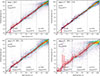 |
Fig. 5. Predicted age versus input age in different magnitude bins. The median μ and σNMAD of the residuals (Δ= output – input) are reported for the full sample and for the three age ranges delimited by the dashed vertical lines. Red points indicate the median values in age bins, with red error bars showing the interquartile range (25th to 75th percentiles) of the distribution. Symbols are colour-coded by number density (more populated regions are plotted in yellow). The upper-left panel shows the results for all the test sample, while the other three panels are limited to a given i magnitude bin, stated in the legend. The typical S/N in the narrow-band filters is also reported. |
A similar analysis is shown in Fig. 6 for the [M/H] estimates for all galaxies with i < 22.5 mag. The median bias and scatter are small (μ= −0.02 dex, σNMAD= 0.29 dex). However, we note that there is a flattening of the predictions at the lowest and highest [M/H] values; namely, the NN tends to overestimate the metallicity in the low-metallicity regime and underestimate it at the high end. Figure 6 also shows the comparison between the input and the predicted E(B-V) values. In this case, the results are excellent, with a median bias close to zero and a small scatter (σNMAD = 0.04 mag).
4.1. Summary of the metrics
We quantified the deviation of our predictions from the one-to-one relation by computing the Pearson correlation coefficient (shown in Fig. 7 as a function of the observed magnitude (equivalent to S/N) for each of the SP parameters) together with the bias, scatter, and fraction of outliers7. As for the age estimates, there is a clear dependence of all these metrics on the S/N of the synthetic photometry. While this result may seem obvious, it is an important indication that our NN model is learning from the real signal (i.e. without over-fitting); thus, it clearly has more trouble with making predictions on noisy SEDs. Given the trends with the ‘observed’ magnitudes, we conclude that our NN-model predictions are robust up to i < 20 mag and could be used (with caution) for fainter galaxies.
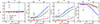 |
Fig. 7. Summary of the metrics (from left to right, median bias, scatter, fraction of outliers, and Pearson coefficient) in bins of of ‘observed’ magnitude in the i-band (and average S/N in the narrow-band filters) for the age (green), metallicity (blue), and dust attenuation (red) predictions. The empty circles are the metrics obtained by means of SED-fitting (details in Sect. 5.1) on the i∼ 17 mag bin, highlighting the improved performance of the NN estimates. |
Comparing the predictions of the different parameters, [M/H] shows the largest scatter and fraction of outliers, along with the smallest Pearson coefficient at all magnitudes, while E(B-V) seems to be the easiest parameter to recover, with a Pearson correlation coefficient above 0.8 and a fraction of outliers < 20%, even for the faintest magnitude bins.
It is especially remarkable the ability of the NN to properly recover the dust attenuation, despite the lack of infrared coverage with J-PAS data. Dust attenuation primarily affects the blue–optical regime of galaxy SEDs and so, the inclusion of near-infrared data is often advocated to help break the age-metallicity-dust degeneracy. While J-PAS does not include NIR photometry beyond 1μm, its contiguous narrow-band coverage and numerous age- and metallicity-sensitive features (e.g. the 4000 Å break, Balmer lines, and metal absorption features) allow us to recover robust estimates of dust attenuation. These results suggest that despite the absence of infrared data, the essential information to constrain dust attenuation is effectively encoded within the J-PAS optical photometry.
4.2. Degeneracies
A well-known challenge when estimating SP parameters from photometry is the intrinsic degeneracy between age, metallicity, and dust attenuation, as all three tend to affect the observed SED in similar ways (i.e. typically making it redder; see detailed discussion in Díaz-García et al. 2015). While such physical parameter degeneracies can be alleviated using spectral features in spectroscopic data (e.g. Domínguez Sánchez et al. 2019a, 2020; Bernardi et al. 2019), they are more difficult to address when using photometry, since the filter convolution washes out those small differences. In SED-fitting methods, all SP parameters must be fitted simultaneously. This requires identifying the spectral template, characterised by a specific age, metallicity, and dust attenuation, which best reproduces the data. Selecting a template with an age that is too old may require compensating by choosing a lower metallicity or a less dust-attenuated model; otherwise, the resulting spectrum would appear too red. One of the key advantages of the methodology presented in this work is that these three parameters are estimated independently using NNs trained specifically to recover each parameter, without the need to fix the others. In other words, the NN that predicts age is agnostic to the values of metallicity and dust attenuation predicted by the other NNs. As a result, the traditional notion of parameter degeneracy (i.e. the correlation between errors in the predicted quantities) is largely mitigated in the context of our approach.
To study possible correlations among the derived stellar population parameters, Fig. 8 shows the parameter space of the differences between the input and predicted parameters across all possible configurations. The data distribution look uniform, with no evident structure that would indicate correlations in the parameter estimate errors. In particular, the age–metallicity parameter space is well behaved, centred around (0,0), and shows no clear dependence on dust attenuation. When E(B–V) is shown on the y-axis, some structure emerges in the form of horizontal bands, related to the discrete sampling of E(B–V) values in the SSP models, but not due to degeneracies in the SSP estimates. Using a finer E(B–V) grid in the training and test samples would likely reduce this effect. A weak residual trend is visible in the E(B-V) versus age plot (where the metallicity increases from left to right) and in the E(B-V) versus [M/H] plot (where the age increases from the bottom to top). These patterns are more prominent outside the 2σ contours and are mostly driven by the faintest galaxies, suggesting mild degeneracies between age, metallicity, and dust attenuation in the low-S/N regime.
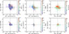 |
Fig. 8. Left: Difference in the predicted metallicity versus age difference, colour-coded by dust attenuation. Middle: Difference in the predicted dust attenuation versus age difference, colour coded by metallicity. Right: Difference in the predicted dust attenuation versus metallicity difference, colour coded by age. Upper panels show galaxies with i < 20.5 mag, bottom panels galaxies with i < 17.0. The white lines show 1, 2, and 3σ contours. |
Indeed, the bottom panels of Fig. 8 show the residuals obtained for the bright sample (i < 17 mag) where these trends are even less pronounced, highlighting a notable contrast with the parameter estimate degeneracies typically seen in SED-fitting, which affect all magnitude ranges (see discussion in Díaz-García et al. 2015). This behaviour suggests that, despite the very similar SED shapes, there is likely a subtle signal in the data that the NN is able to capture, allowing it to accurately recover the ground truth values. This highlights one of the key advantages of NN over traditional SED-fitting methods.
4.3. SSP Model dependence
In this work, we combine synthetic photometry from different SSP libraries to train the NN models. After several tests, we found that the network performs more robustly when information from multiple libraries is mixed. Additionally, incorporating different IMFs, available in the E-MILES SSPs, further enhances the NNs performance. This can be interpreted as a form of data augmentation, helping the network focus on general trends rather than specific features of individual libraries or IMFs.
We combined the three SSP libraries in our training sample, exploring whether there is any dependence of our results on the SSP library for which the predictions are made. For that purpose, Fig. 9 shows the difference between input and output parameters for the three SSP libraries used. In general, all the SSP models behave very well, with almost no bias in all the estimated range. It is worth noting that the metallicities are overestimated for galaxies with [M/H] < −1.5 for the CB19 and XSL models. Also, the ages are slightly overestimated for the youngest SSP models for the E-MILES and XSL libraries. On the contrary, there is no age bias for bias for the CB19 SSP models, nor metallicity bias for E-MILES. We recall the reader that all the templates younger than 30 Myr come precisely from the CB19 library, while the lowest metallicity values are those of the E-MILES library, so these results are not surprising.
The small oscillatory features visible in Fig. 9 probably arise as a result of the division of the test sample into three sub-sets, one for each SSP library, which reduces the statistics and enhances local fluctuations. Since the NN is trained simultaneously with all libraries, these patterns might also trace minor systematic differences among the SSP models (e.g. stellar libraries or isochrone choices). The effect is mainly seen in the individual data points, while the median residuals remain smooth and close to zero, confirming that no significant systematic bias is present in the model predictions.
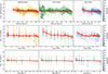 |
Fig. 9. Difference between the predicted and the input parameters from top to bottom: log(Age), [M/H] and E(B-V) for the sample limited to i < 19.5, divided into different SSP synthetic photometry (from left to right: E-MILES, CB19, and XSL). The colour intensity corresponds to the ‘observed’ magnitude. Red points indicate the median values in bins, with red error bars showing the interquartile range (25th to 75th percentiles) of the distribution. |
5. Discussion
Predicting SP parameters from photometry is an extensively investigated topic and doing a full review is not the purpose of this work. Making a fair comparison of the performance of our results with other methodologies such as SED-fitting is not trivial, given the differences in the photometry, stellar population models, and parametrisation of the SFHs. In this section, we compare our results with those obtained by SED-fitting on the same synthetic photometry test sample. We also compare our results with those in the literature whose analyses are comparable, to some extent, to the analysis presented here.
5.1. Comparison with SED fitting
The most common approach to derive SP parameters from photometry is by means of an SED fitting. To compare our methodology with SED fitting procedure in a fair way, we fit the exact same synthetic photometry of the test sample using the CB19 models with CIGALE SED-fitting code. To be more conservative, we only do this exercise for the test sample coming from the CB19 library. We assumed the SFHs to be similar to SSPs (i.e. a single burst very short formation timescale, τ = 1 Myr) with a fine grid of possible age, metallicity8, and dust attenuation values, as described in Table 2, with no nebular lines and with the Cardelli et al. (1989) attenuation law. The results are shown in Fig. 7 as empty circles. For simplicity, we limit our analysis to photometric errors typical from mag ∼ 17 galaxies. We obtained the median bias, scatter, and percentage of outliers: μ= (0.14 dex, 0.22 dex, −0.02 mag), σNMAD= (0.30 dex, 0.40 dex, 0.06 mag), and fo= (40%, 56%, 4%) at i∼ 17 mag for the age, metallicity, and dust attenuation, respectively. It is clear that, for the three SP parameters, all the metrics reported are worse for SED-fitting estimates (the detailed one-to-one comparison is shown in Fig. D.1). This confirms that NN are a very powerful tool for inferring the SP properties of galaxies and encourages us to continue exploring their use, despite the limitations discussed in Sect. 7.
Parameter space covered by the CB19 models used in the SED-fitting procedure with CIGALE.
5.2. Comparison with literature
González Delgado et al. (2021) compared the results of the parametric SED-fitting code BAYSEAGAL on the mini-JPAS sample with the output of three non-parametric SED-fitting codes: MUFFIT, ALSTAR, and TGASPEX (Magris et al. 2015). They concluded that given the differences in the different SED-fitting approaches, the precision of the SP properties depends on the S/N and the property with the largest uncertainty is the metallicity, in agreement with our results.
In Mejía-Narváez et al. (2017), the authors report results of SED-fitting on mock observations from the Synthetic Spectral Atlas of Galaxies, including spectroscopy, narrow-band photometry, and broad-band photometry. The narrow-band photometry is aimed at reproducing J-PAS observations with different levels of noise and the SP parameters are estimated using the DYNBAS non-parametric spectral fitting code (Magris et al. 2015). They reported values of bias and scatter of μ= (−0.01, −0.01, −0.016) σ= (0.2, 0.17, 0.2) for log t, log Z, and Av, respectively, which are comparable to our results. However, we should note that their mock observations include SFHs that are more complex than SSP and their fitting used the library of Bruzual & Charlot (2003). Liew-Cain et al. (2021) trained a convolutional neural network on synthetic J-PAS photometry from 21 000 spectra of a sample of 200 galaxies from the CALIFA survey (Sánchez et al. 2012, CALIFA) with mB∼ 18 mag. The authors assumed the ‘true’ metallicity and age were the values those obtained by means of a full spectral fitting on the emission-line cleaned spectra with STECKMAP code (Ocvirk et al. 2006). They reported a very small bias and a standard deviation σ ∼ 0.2 dex for both log(age) [yr] and Z, comparable to our results (see Fig. 7), despite the fact that the age and metallicity parameter space targeted in that work is much more limited than ours (log t [yr] = [9.2, 10] and [M/H] = [−0.6, 0.2]). In a recent work, Wang et al. (2024) trained a convolutional NN (CNN) to predict SP parameters from Sloan Digital Sky Survey (SDSS) spectra, using the values obtained by full spectral fitting with PPXF the as ‘labels’. They obtained a scatter σ∼ 0.11 for the age and metallicity and σ∼ 0.018 for the E(B-V). Although these values are smaller than the ones we obtained here, we note that those were estimated using spectroscopic information for a bright sample of galaxies (r∼ 18). We would like to emphasise that none of the aforementioned studies compares their results to the ground truth, as we do in this work. Instead, they assess the performance against SP parameters derived from alternative methods, such as spectral fitting, which inherently carry their own uncertainties and biases that can propagate into the evaluation of the results.
In a comprehensive study that uses information from simulations as ground truth, Woo et al. (2024) compared the performance of several popular spectral fitting codes with that of a CNN (STARNET) using mock spectra from IllustrisTNG-100 simulations (Nelson et al. 2019) mimicking SDSS. Although their results are not directly comparable to ours given the large differences in S/N and spectral resolution, they found that STARNET vastly outperforms conventional codes, supporting our findings on the power of machine learning based methods for deriving SP parameters.
5.3. Caveats
Although the results are very promising, there are a few caveats to our current approach that should be noted. First, the SSP models used to train the neural network are all at redshift z = 0. Given the narrow width of the J-PAS filters (∼ 150 Å), the redshift bins required to accurately sample the synthetic photometry are approximately Δz ∼ 0.03. While generating synthetic photometry up to z ∼ 1 is feasible, it would significantly increase the computational cost of our method and we leave this to a future work. Additionally, as already mentioned in this work, our training sample does not include emission lines or complex SFHs, which are very common in the Local Universe. The performance of the neural network when applied to composite stellar populations (CSPs) is discussed in Appendix C. As expected, the accuracy of the predicted properties decreases with the complexity of the CSP, with the poorest results obtained for models with a constant SFH. This is in agreement with previous works (e.g. Breda et al. 2022), which have shown that age estimates are biased when nebular continuum emission is not taken into account. An alternative would be to use simulation based inference on non-parametric SFHs, as done in Iglesias-Navarro et al. (2024) for early-type galaxies with spectroscopic data. Finally, the current approach is not optimised for missing data. Since the NN is trained in fluxes, missing data in the strict sense do not occur. Issues such as masking or bad pixels could be overcome by linearly interpolating neighbouring filters, which preserves the accuracy of the derived parameters as long as the fraction of missing bands remains small (Hernán-Caballero et al. in prep.). The number of J-PAS sources in the public EDR with observations in all bands is 71%.
We leave these improvements to a future work and present our results as a promising proof of concept, highlighting the power of combining J-PAS narrow-band photometry and state-of-the-art synthetic stellar population libraries with deep learning inference.
6. Testing on J-PAS galaxies
The first J-PAS data release was made public in 2024 (Vázquez Ramió in prep.). We used the released J-PAS photometry to compute the stellar population properties for a sample of local galaxies from the NN predictions. We have made a selection of low-z galaxies with spectroscopic redshift zspec < 0.1 (and |zphot − zspec|< 0.005)9, i < 20 mag, resulting in 1478 galaxies. We use as input for the NN predictions the APER_COR_3_0_FLUX values10, normalised by their mean. In Fig. 10, we present the projection of both synthetic and real photometry onto a 2D parameter space using UMAP (McInnes et al. 2020), a non-linear dimensionality reduction technique that preserves both local and global structure, making it well-suited for visualising complex, high-dimensional datasets in 2D.
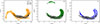 |
Fig. 10. Projection of the synthetic photometry and the real J-PAS photometry in the 2D parameter space obtained by UMAP dimensionality reduction algorithm. Black and gray data show the J-PAS APER_COR_3_0 and AUTO fluxes, respectively, while each panel shows the synthetic photometry for the three SSP libraries used in the training of the NN (E-MILES in orange, CB19 in green, and XSL in blue). While a single library does not fully cover the parameter space observed in real J-PAS data, the coverage is notably improved when the three libraries are combined together. |
The overlap between the real observations and the synthetic photometry in the 2D UMAP projection suggests that both datasets span a similar region of parameter space. While 2D projections cannot capture all aspects of the high-dimensional structure (i.e. it does not guarantee the consistency between the modelled and real data distributions) when using only a single SSP library, the synthetic models fail to fully cover the range of colours observed in the J-PAS data, implying a genuine mismatch in the original, higher dimensional space. On the other hand, when combining the three SSP libraries, the synthetic photometry achieves significantly better coverage, aligning more closely with the observed data. This supports the strategy of integrating all three libraries into the training sample, as it enhances the robustness and generalisation of the neural network.
We applied the NN models trained on synthetic photometry to the J-PAS observations and we compare our results with those derived from SED-fitting using MUFFIT with two-burst CSP with CB17 models and Chabrier IMF (more details in Díaz-García, in prep.). For this exercise, we used more restrictive criteria for the redshift limit (z < 0.03) and for the photometric quality, avoiding galaxies close to bright stars (FLAGS_MASK = 2) or with all the bands having bad FLAGs, resulting in a sample of 90 galaxies.
In Fig. 11, we present the NN predicted ages, metallicities, and dust attenuation compared to the MUFFIT SED-fitting results. The NN predictions yield reasonable values, with ages spanning from very young to very old stellar populations (although a few of them have non-physically old ages > 12 Gyr), sub-solar metallicities, and intermediate E(B-V) values peaking around 0.2 mag. Compared to the SED-fitting results, significant differences arise, namely, the SED-fitting age predictions are systematically younger, clustered around ∼2 Gyr, while the metallicity estimates are systematically higher and the E(B-V) values exhibit a more similar distribution across both methods, although the one-to-one-agreement is far from excellent. We recall that the NN is trained to predict SSP while the SED-fitting from Díaz-García et al. (in prep.) uses two-burst CSP, so the discrepancy between the two approaches is expected.
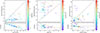 |
Fig. 11. Age (left, colour-coded by metallicity), metallicity (middle, colour-coded by age), and dust attenuation (right, colour-coded by age) NN predictions versus MUFFIT SED-fitting predictions from Díaz-García (in prep.) for a sample of observed J-PAS galaxies. |
Interestingly, the NN predicts notably low metallicity values for the observed galaxies, which stands in contrast to the bias direction seen in the test sample (see Fig. 6). The location of many of the J-PAS galaxies does fall into the low-metallicity and old-age region of the UMAP parameter space (see Fig. E.1). One of the possible explanation for such low metallicity estimates could be related to the presence of emission lines, which are not included in the training sample. Indeed, ∼25% of the galaxies with NN predicted [M/H] < −1.5 have emission lines with S/N > 3 (Fernández-Ontiveros et al. in prep.). An alternative explanation involves more complex SFHs, where recent star formation leads to bluer colours. This could influence the metallicity estimates and it is, in fact, consistent with the predictions for CSP outlined in Appendix C. In addition, subtle calibration differences between the synthetic and observed photometry could also impact the NN estimates (see Boris et al. 2007). This result underscores the importance of carefully considering the limitations of NN models trained on data that differ from the target observations, as a caveat against their blind application. We leave the inclusion of more complex SFHs or emission lines in the training sample to a future work, due to the complexity of properly modelling the nebular component.
7. Conclusions
In this work, we present a NN to estimate SP properties (e.g. age, metallicity, and dust attenuation) of galaxies from J-PAS photometry. The NN is trained with synthetic photometry from SSP models from three state-of-the-art popular libraries (E-MILES, XSL, and CB19). We added realistic noise to the synthetic photometry by applying Gaussian variations with an amplitude of typical errors in the mini-JPAS data. Our main conclusions are listed below.
-
The properties estimated by the NN on the test sample are accurate, but also highly dependent on the S/N of the synthetic photometry. For i ∼ 17 mag, we obtained median bias μ= (0.01, 0.00, 0.00), scatter σNMAD= (0.23 dex, 0.29 dex, 0.04 mag), percentage of outliers fo= (17%, 24%, 1%), and Pearson coefficient P= (98, 95, 98), for log t [yr], [M/H] and E(B-V), respectively (see Fig. 7).
-
The NN estimates on the test sample (limited to galaxy spectra built from the CB19 library) outperformed the SED-fitting for all the parameters and metrics (see Fig. 7), demonstrating the great potential of NN for SSP derivation.
-
One of the advantages of this approach is that age, metallicity and dust attenuation are derived independently and, indeed, we observed no evident correlations in the prediction errors on the age-dust-metallicity planes (see Fig. 8).
-
We found no clear dependence on the performance of the NN when applied to different SSP libraries (see Fig. 9), except for very low ages and metallicities.
-
Combining the three SSP libraries provides better results than training the NN with a single library. It also improves the overlap between real J-PAS observations and synthetic photometry in the 2D UMAP parameter space (see Fig. 10).
-
When applied to J-PAS photometry of real galaxies, the NN predicted metallicities are significantly lower than those estimated via SED-fitting using two-burst CSP (see Fig. 11), whereas the ages are systematically younger.
-
Possible reasons for this discrepancy are discussed in Sect. 5.3, including the presence of emission lines (affecting approximately ∼25% of the galaxies with predicted [M/H] < 1–1.5), calibration differences between the synthetic and observed photometry, the effect of redshift, or the existence of more complex SFHs than those represented in the training set. Several of these obstacles would be mitigated in the analysis of globular clusters.
Despite these challenges, this pilot study demonstrates the strong potential of NN for estimating SSP parameters from photometric data. The method demonstrates a reliable performance across a wide magnitude range and offers a flexible foundation that can be extended to more complex and realistic scenarios. Future improvements, such as incorporating emission lines, more diverse SFHs, and observed-frame effects, will further enhance its applicability to current and upcoming large photometric surveys.
Acknowledgments
HDS acknowledges financial support by RyC2022-030469-I grant, funded by MCIU/AEI/10.13039/501100011033 and FSE+ and the Spanish Ministry of Science and Innovation and the European Union – NextGenerationEU through the Recovery and Resilience Facility project ICTS-MRR-2021-03-CEFCA and financial support provided by the Governments of Spain and Aragón through their general budgets and the Fondo de Inversiones de Teruel. PC acknowledges support from Conselho Nacional de Desenvolvimento Científico e Tecnológico (CNPq) under grant 310555/2021-3 and from Fundação de Amparo à Pesquisa do Estado de São Paulo (FAPESP) process number 2021/08813-7. This research has made use of the SVO Filter Profile Service “Carlos Rodrigo”, funded by MCIN/AEI/10.13039/501100011033/ through grant PID2023-146210NB-I00. The authors gratefully acknowledge the computer resources at Artemisa, funded by the European Union ERDF and Comunitat Valenciana as well as the technical support provided by the Instituto de Física Corpuscular, IFIC (CSIC-UV). L.A.D.G. acknowledges financial support from the State Agency for Research of the Spanish MCIU through ‘Center of Excellence Severo Ochoa’ award to the Instituto de Astrofísica de Andalucía (CEX2021-001131-S) funded by MCIN/AEI/10.13039/501100011033 and to PID2022-141755NB-I00. J.M.V. acknowledges financial support from the Spanish AEI grant PID2022-136598NB-C32. I.B. has received funding from the European Union’s Horizon 2020 research and innovation programme under the Marie Sklodowska-Curie Grant agreement ID n.° 101059532. SGL acknowledges the financial support from the MICIU with funding from the European Union NextGenerationEU and Generalitat Valenciana in the call Programa de Planes Complementarios de I + D + i (PRTR 2022) Project (VAL-JPAS), reference ASFAE/2022/025. This work is part of the research Project PID2023-149420NB-I00 funded by MICIU/AEI/10.13039/501100011033 and by ERDF/EU. This work is also supported by the project of excellence PROMETEO CIPROM/2023/21 of the Conselleria de Educación, Universidades y Empleo (Generalitat Valenciana). AAC acknowledges financial support from the Severo Ochoa grant CEX2021- 001131-S funded by MCIN/AEI/10.13039/501100011033 and from the project PID2023-153123NB-I00, funded by MCIN/AEI. The work of V.M.P. is supported by NOIRLab, which is managed by the Association of Universities for Research in Astronomy (AURA) under a cooperative agreement with the U.S. National Science Foundation. GB acknowledges financial support from Universidad Nacional Autónoma de México through grants DGAPA/PAPIIT IG100319, BG100622 and IN106124. Partially based on observations made with the JST250 telescope and JPCam at the Observatorio Astrofísico de Javalambre (OAJ), in Teruel, owned, managed, and operated by the Centro de Estudios de Física del Cosmos de Aragón (CEFCA). We acknowledge the OAJ Data Processing and Archiving Department (DPAD) for reducing and calibrating the OAJ data used in this work. Funding for the J-PAS Project has been provided by the Governments of Spain and Aragón through the Fondo de Inversiones de Teruel; the Aragonese Government through the Research Groups E96, E103, E16_17R, E16_20R, and E16_23R; the Spanish Ministry of Science and Innovation (MCIN/AEI/10.13039/501100011033 y FEDER, Una manera de hacer Europa) with grants PID2021-124918NB-C41, PID2021-124918NB-C42, PID2021-124918NA-C43, and PID2021-124918NB-C44; the Spanish Ministry of Science, Innovation and Universities (MCIU/AEI/FEDER, UE) with grants PGC2018-097585-B-C21 and PGC2018-097585-B-C22; the Spanish Ministry of Economy and Competitiveness (MINECO) under AYA2015-66211-C2-1-P, AYA2015-66211-C2-2, and AYA2012-30789; and European FEDER funding (FCDD10-4E-867, FCDD13-4E-2685). The Brazilian agencies FINEP, FAPESP, FAPERJ and the National Observatory of Brazil have also contributed to this project. Additional funding was provided by the Tartu Observatory and by the J-PAS Chinese Astronomical Consortium.
References
- Bellstedt, S., Robotham, A. S. G., Driver, S. P., et al. 2020, MNRAS, 498, 5581 [NASA ADS] [CrossRef] [Google Scholar]
- Benitez, N., Dupke, R., & Moles, M., et al. 2014, ArXiv e-prints [arXiv:1403.5237] [Google Scholar]
- Bernardi, M., Domínguez Sánchez, H., Brownstein, J. R., Drory, N., & Sheth, R. K. 2019, MNRAS, 489, 5633 [Google Scholar]
- Bom, C. R., Cortesi, A., Ribeiro, U., et al. 2024, MNRAS, 528, 4188 [NASA ADS] [CrossRef] [Google Scholar]
- Bonoli, S., Marín-Franch, A., Varela, J., et al. 2021, A&A, 653, A31 [NASA ADS] [CrossRef] [EDP Sciences] [Google Scholar]
- Boquien, M., Burgarella, D., Roehlly, Y., et al. 2019, A&A, 622, A103 [NASA ADS] [CrossRef] [EDP Sciences] [Google Scholar]
- Boris, N. V., Sodré, L., Jr., Cypriano, E. S., et al. 2007, ApJ, 666, 747 [NASA ADS] [CrossRef] [Google Scholar]
- Breda, I., Vilchez, J. M., Papaderos, P., et al. 2022, A&A, 663, A29 [NASA ADS] [CrossRef] [EDP Sciences] [Google Scholar]
- Bruzual, G., & Charlot, S. 2003, MNRAS, 344, 1000 [NASA ADS] [CrossRef] [Google Scholar]
- Cappellari, M., & Emsellem, E. 2004, PASP, 116, 138 [Google Scholar]
- Cappellari, M., Emsellem, E., Krajnović, D., et al. 2011, MNRAS, 413, 813 [Google Scholar]
- Cardelli, J. A., Clayton, G. C., & Mathis, J. S. 1989, ApJ, 345, 245 [Google Scholar]
- Chabrier, G. 2003, ApJ, 586, L133 [NASA ADS] [CrossRef] [Google Scholar]
- Cid Fernandes, R., Mateus, A., Sodré, L., Stasińska, G., & Gomes, J. M. 2005, MNRAS, 358, 363 [Google Scholar]
- Cid Fernandes, R., Mateus, A., Sodré, L., Stasinska, G., & Gomes, J. M. 2011, Astrophysics Source Code Library [record ascl:1108.006] [Google Scholar]
- del Pino, A., López-Sanjuan, C., Hernán-Caballero, A., et al. 2024, A&A, 691, A221 [NASA ADS] [CrossRef] [EDP Sciences] [Google Scholar]
- Díaz-García, L. A., Cenarro, A. J., López-Sanjuan, C., et al. 2015, A&A, 582, A14 [Google Scholar]
- Domínguez Sánchez, H., Pérez-González, P. G., Esquej, P., et al. 2016, MNRAS, 457, 3743 [Google Scholar]
- Domínguez Sánchez, H., Huertas-Company, M., Bernardi, M., Tuccillo, D., & Fischer, J. L. 2018, MNRAS, 476, 3661 [Google Scholar]
- Domínguez Sánchez, H., Bernardi, M., Brownstein, J. R., Drory, N., & Sheth, R. K. 2019a, MNRAS, 489, 5612 [CrossRef] [Google Scholar]
- Domínguez Sánchez, H., Huertas-Company, M., Bernardi, M., et al. 2019b, MNRAS, 484, 93 [Google Scholar]
- Domínguez Sánchez, H., Bernardi, M., Nikakhtar, F., Margalef-Bentabol, B., & Sheth, R. K. 2020, MNRAS, 495, 2894 [CrossRef] [Google Scholar]
- Domínguez Sánchez, H., Martin, G., Damjanov, I., et al. 2023, MNRAS, 521, 3861 [CrossRef] [Google Scholar]
- Eftekhari, E., Vazdekis, A., & La Barbera, F. 2021, MNRAS, 504, 2190 [CrossRef] [Google Scholar]
- Galarza, C. A., Daflon, S., Placco, V. M., et al. 2022, A&A, 657, A35 [NASA ADS] [CrossRef] [EDP Sciences] [Google Scholar]
- Girardi, L., Bressan, A., Bertelli, G., & Chiosi, C. 2000, A&AS, 141, 371 [NASA ADS] [CrossRef] [EDP Sciences] [Google Scholar]
- Gonçalves, G., Coelho, P., Schiavon, R., & Usher, C. 2020, MNRAS, 499, 2327 [Google Scholar]
- González Delgado, R. M., Díaz-García, L. A., de Amorim, A., et al. 2021, A&A, 649, A79 [Google Scholar]
- Gurung-López, S., Gronke, M., Saito, S., Bonoli, S., & Orsi, Á. A. 2022, MNRAS, 510, 4525 [NASA ADS] [CrossRef] [Google Scholar]
- Gurung-López, S., Byrohl, C., Gronke, M., et al. 2025, A&A, 698, A139 [NASA ADS] [CrossRef] [EDP Sciences] [Google Scholar]
- Hernán-Caballero, A., Alonso-Herrero, A., Pérez-González, P. G., et al. 2013, MNRAS, 434, 2136 [Google Scholar]
- Hernán-Caballero, A., Alonso-Herrero, A., Pérez-González, P. G., et al. 2014, MNRAS, 443, 3538 [CrossRef] [Google Scholar]
- Hernán-Caballero, A., Varela, J., López-Sanjuan, C., et al. 2021, A&A, 654, A101 [NASA ADS] [CrossRef] [EDP Sciences] [Google Scholar]
- Huertas-Company, M., & Lanusse, F. 2023, PASA, 40, e001 [NASA ADS] [CrossRef] [Google Scholar]
- Iglesias-Navarro, P., Huertas-Company, M., Martín-Navarro, I., Knapen, J. H., & Pernet, E. 2024, A&A, 689, A58 [NASA ADS] [CrossRef] [EDP Sciences] [Google Scholar]
- Johnson, B. D., Leja, J., Conroy, C., & Speagle, J. S. 2021, ApJS, 254, 22 [NASA ADS] [CrossRef] [Google Scholar]
- Kaeufer, T., Woitke, P., Min, M., Kamp, I., & Pinte, C. 2023, A&A, 672, A30 [NASA ADS] [CrossRef] [EDP Sciences] [Google Scholar]
- Kroupa, P. 2001, MNRAS, 322, 231 [NASA ADS] [CrossRef] [Google Scholar]
- Leja, J., Carnall, A. C., Johnson, B. D., Conroy, C., & Speagle, J. S. 2019, ApJ, 876, 3 [Google Scholar]
- Liew-Cain, C. L., Kawata, D., Sánchez-Blázquez, P., Ferreras, I., & Symeonidis, M. 2021, MNRAS, 502, 1355 [NASA ADS] [CrossRef] [Google Scholar]
- Magris, C. G., Mateu, P. J., Mateu, C., et al. 2015, PASP, 127, 16 [NASA ADS] [CrossRef] [Google Scholar]
- Martínez-Solaeche, G., González Delgado, R. M., García-Benito, R., et al. 2022, A&A, 661, A99 [NASA ADS] [CrossRef] [EDP Sciences] [Google Scholar]
- Martínez-Solaeche, G., Queiroz, C., González Delgado, R. M., et al. 2023, A&A, 673, A103 [NASA ADS] [CrossRef] [EDP Sciences] [Google Scholar]
- McInnes, L., Healy, J., & Melville, J. 2020, UMAP: Uniform Manifold Approximation and Projection for Dimension Reduction [Google Scholar]
- Mejía-Narváez, A., Bruzual, G., Magris, C. G., et al. 2017, MNRAS, 471, 4722 [Google Scholar]
- Nelson, D., Springel, V., Pillepich, A., et al. 2019, Comput. Astrophys. Cosmol., 6, 2 [Google Scholar]
- Ocvirk, P., Pichon, C., Lançon, A., & Thiébaut, E. 2006, MNRAS, 365, 74 [Google Scholar]
- Pietrinferni, A., Cassisi, S., Salaris, M., & Castelli, F. 2004, ApJ, 612, 168 [Google Scholar]
- Plat, A., Charlot, S., Bruzual, G., et al. 2019, MNRAS, 490, 978 [Google Scholar]
- Robotham, A. S. G., Bellstedt, S., Lagos, C. d. P., et al. 2020, MNRAS, 495, 905 [NASA ADS] [CrossRef] [Google Scholar]
- Rodrigo, C., Cruz, P., Aguilar, J. F., et al. 2024, A&A, 689, A93 [NASA ADS] [CrossRef] [EDP Sciences] [Google Scholar]
- Salpeter, E. E. 1955, ApJ, 121, 161 [Google Scholar]
- Sánchez, S. F., Kennicutt, R. C., Gil de Paz, A., et al. 2012, A&A, 538, A8 [Google Scholar]
- Serra, P., & Trager, S. C. 2007, MNRAS, 374, 769 [Google Scholar]
- Serven, J., Worthey, G., & Briley, M. M. 2005, ApJ, 627, 754 [NASA ADS] [CrossRef] [Google Scholar]
- Thomas, D., Maraston, C., Bender, R., & de Oliveira, C. M. 2005, ApJ, 621, 673 [NASA ADS] [CrossRef] [Google Scholar]
- Trager, S. C., & Somerville, R. S. 2009, MNRAS, 395, 608 [Google Scholar]
- Trager, S. C., Faber, S. M., Worthey, G., & González, J. J. 2000, AJ, 119, 1645 [Google Scholar]
- Vazdekis, A., Sánchez-Blázquez, P., Falcón-Barroso, J., et al. 2010, MNRAS, 404, 1639 [NASA ADS] [Google Scholar]
- Vazdekis, A., Koleva, M., Ricciardelli, E., Röck, B., & Falcón-Barroso, J. 2016, MNRAS, 463, 3409 [Google Scholar]
- Verro, K., Trager, S. C., Peletier, R. F., et al. 2022a, A&A, 661, A50 [NASA ADS] [CrossRef] [EDP Sciences] [Google Scholar]
- Verro, K., Trager, S. C., Peletier, R. F., et al. 2022b, A&A, 660, A34 [NASA ADS] [CrossRef] [EDP Sciences] [Google Scholar]
- Walmsley, M., Lintott, C., Géron, T., et al. 2022, MNRAS, 509, 3966 [Google Scholar]
- Wang, C., Bai, Y., López-Sanjuan, C., et al. 2022, A&A, 659, A144 [Google Scholar]
- Wang, L.-L., Yang, G.-J., Zhang, J.-L., et al. 2024, MNRAS, 527, 10557 [Google Scholar]
- Whitten, D. D., Placco, V. M., Beers, T. C., et al. 2019, A&A, 622, A182 [NASA ADS] [CrossRef] [EDP Sciences] [Google Scholar]
- Woo, J., Walters, D., Archinuk, F., et al. 2024, MNRAS, 530, 4260 [NASA ADS] [CrossRef] [Google Scholar]
The E(B-V) values used in this work are 0, 0.03, 0.06, 0.13, 0.26, 0.40, 0.60 and 0.80.
Obtained from http://svo2.cab.inta-csic.es/theory/fps/; see Rodrigo et al. (2024).
Mini-JPAS is a 1 deg2 survey of the AEGIS field observed with 56 J-PAS filters on the Pathfinder camera. More details in Bonoli et al. (2021).
We transform magnitude errors in the S/N following the formula S/N = 2.5/ln(10)Δm.
In yr in logarithmic scale.
Following Kaeufer et al. (2023).
Defined as those objects for which the difference between the input and the output is > 0.25 dex/mag.
Noting that we use all the allowed metallicity values in CIGALE for these exercise.
We require zphot and zspec to agree as a way to confirm that the spectroscopic redshift is correct and that there are no strong artifacts in the photometry that would affect the SP estimates.
The results are not severely affected when using AUTO photometry.
Appendix A: Optimisation of NN hyper-parameters
Neural network hyper-parameters can have a significant impact on model performance; however, exploring the full hyper-parameter space is computationally expensive and often impractical. For this reason, we limited our investigation to a representative set of configurations detailed in section 3. These included variations in the NN architecture (base-NN or SED-NN), batchsize (32, 100, and 1000), and the inclusion of dropout. The performance of each setup, reported as the metrics obtained for the predicted stellar population parameters as a function of magnitude (similar to Fig.7) is summarised in Fig A.1. The main differences are seen in the bias values, while the fraction of outliers or Pearson/R2 coefficients are less affected by the hyper-parameter choice. Throughout the paper, we show the results obtained with the base-NN model with a batchsize = 32 (red line).
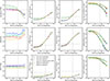 |
Fig. A.1. Comparison of the metrics (bias, scatter, fraction of outliers and Pearson (dashed line) and R2 (thick line) coefficients (from left to right) for different parameters (age, metallicity, and E(B-V) (top to bottom) as a function of galaxy i-band magnitude, obtained for different training strategies, as stated in the legend (details in Sect. 3). |
Appendix B: Loss curves
Figure B.1 reports the loss curves for the optimal models to illustrate the training dynamics, displaying a very similar behaviour between the training and validation sets. In particular, the E(B–V) model displays an excellent agreement, while the age and [M/H] models show a mild tendency towards over-fitting, with the training loss shown to be slightly lower than the validation loss. However, the differences remain small (≤ 0.1 in MSE) and do not significantly affect the model performance (we have checked and the differences between the predictions of the ‘best’ model that minimises the loss in the validation sample and the final models are negligible.
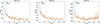 |
Fig. B.1. Loss curves (loss function as a function of training epoch) for the train (blue) and validation (orange) samples for the age (left), metallicity (middle), and dust attenuation (right) NN models. |
Appendix C: Test on Composite stellar populations
The NN presented in this work are trained with SSP models, which are a simplistic approximation of the SFHs of real galaxies. To assess the impact of our estimates on more complex SFHs, we use a set of composite stellar population (CSP) models consisting of
-
three 1 Gyr bursts with different metallicities (Z = 0.04, 0.08, 0.17);
-
an initial 1 Gyr burst at t = 0 with metallicity Z = 0.008 followed by a second 1 Gyr burst at different ages (1, 4, 7, and 10 Gyr) and with Z = 0.017;
-
a constant SFR with metallicity Z = 0.017
No dust attenuation is applied to avoid further degeneracies. Fig. C.1 shows the NN predictions for these CSP. The predictions for the 1 Gyr burts (upper panel) show a significant dependence on the metallicity, being more robust for the highest metallicity case (Z = 0.017, red line). For the other two metallicities, the ages are usually under-predicted (specially for Z = 0.008), while the metallicities show average deviations of ∼ 0.5 dex (up to 1dex for the Z = 0.008 case). On the contrary, the dust attenuation is well constrained (E(B-V)∼0) in all cases. The results for the two-burst CSP are a bit more complex (middle panel). In general, ages are under-predicted, but metallicities are constrained within ∼ 0.5 dex. Interestingly, both the age and E(B-V) predictions show clear fluctuations ∼ 2 Gyr after the second burst takes place (marked as dashed vertical line). Finally, for the constant SFR case (lower panel), none of the parameters is well constrained, specially after 2Gyr. The metallicity is unpredicted (≳ 0.5), the dust attenuation over-predicted (up to 0.2 mag difference) and the predicted age is always ∼ 0. Since the NN was trained on SSP, the challenges encountered when recovering the properties of CSPs are not unexpected. Rather than a limitation, this points to a clear direction for future work: incorporating more complex and realistic SFHs into the train and test datasets to improve the model’s performance on more representative galaxy populations.
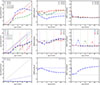 |
Fig. C.1. NN predictions for different CSP models -from top to bottom: 1 Gyr bursts, two 1 Gyr bursts, constant SFR (colours correspond to different flavours, as stated in the legend). Age, metallicity, and dust attenuation predictions are shown (left to right). The dashed lines show the light-weighted ages, metallicities, or E(B-V). The vertical dashed lines in the middle panel show the time when the second burst takes place. |
Appendix D: SED-fitting plots
In Fig. 7, we compare the metrics summarising the performance of the results obtained by the NN and the SED-fitting with CIGALE on the same test set. To shed more light on the SED-fitting estimates, Fig. D.1 shows the analogue of Figs. 5 and 6 for the CIGALE Bayesian outputs. There is a clear quantisation of the age predictions, the E(B-V) is slightly underestimated and the [M/H] are clearly overestimated for [M/H] < 0.
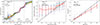 |
Fig. D.1. Same as Fig. 5 and 6 but for the output obtained with CIGALE SED-fitting (see Sect.5.1 for details). |
Appendix E: UMAP properties
In Section 6, the projection of the J-PAS observations in the 2D UMAP parameters space is shown on top of the SSP synthetic photometry. In Fig E.1, we show the projection of the synthetic photometry (combining the three SSP libraries) on the same 2D parameter space, colour-coded by SSP parameters and observed magnitude. Notably, many of the J-PAS galaxies fall within regions occupied by models with low [M/H], suggesting that, in this 2D parameter space, the observed galaxy colours are consistent with those of low-metallicity SSPs. While this does not guarantee that the galaxies’ metallicities are truly so low, it does support the consistency of our methodology with the model’s predictions.
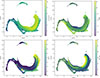 |
Fig. E.1. Projection of the synthetic photometry in the 2D parameters space obtained with UMAP dimensionality reduction algorithms, colour-coded by age (upper left), metallicity (upper right), dust attenuation (bottom left), and observed magnitude (bottom right). |
All Tables
Number of SSP models for the different libraries for the original and the mock samples.
Parameter space covered by the CB19 models used in the SED-fitting procedure with CIGALE.
All Figures
|
Fig. 1. Age-metallicity coverage of the three SSP synthesis models used in this work to train the NNs. The grey symbols (dots and histograms) show the combination of the three SSP libraries. In each panel, we show the individual libraries: E-MILES in orange (left panel), CB19 in green (middle panel), and XSL in blue (right panel). Note: Models with ages < 30 Myr are only included in the CB19 SSP library. |
| In the text | |
|
Fig. 2. Examples of synthetic J-PAS photometry from E-MILES SSP for a young (3 Gyr) and an old (10 Gyr) SSP with different metallicities and dust attenuation, as stated in the legend. Fluxes are normalised to the mean value of the flux for each SSP. Note: Subtle differences need to be distinguished for a proper characterisation of the SSPs (e.g. compare the red and purple lines). |
| In the text | |
|
Fig. 3. Left: Average magnitude error of mini-JPAS galaxies for the 57 filters for different observed magnitudes (16, 18, 20, and 22 mag). Right: Synthetic J-PAS photometry obtained after applying random Gaussian variations consistent with the typical errors at different magnitudes. Colours represent different mock observed magnitudes. The thick dashed black line is the original SED. |
| In the text | |
|
Fig. 4. Age (left panel), metallicity (middle panel) and dust attenuation (right panel) distribution for the training (blue), test (red), and validation (empty black) sub-samples. The sub-samples are randomly selected, showing no differences in their distributions. |
| In the text | |
|
Fig. 5. Predicted age versus input age in different magnitude bins. The median μ and σNMAD of the residuals (Δ= output – input) are reported for the full sample and for the three age ranges delimited by the dashed vertical lines. Red points indicate the median values in age bins, with red error bars showing the interquartile range (25th to 75th percentiles) of the distribution. Symbols are colour-coded by number density (more populated regions are plotted in yellow). The upper-left panel shows the results for all the test sample, while the other three panels are limited to a given i magnitude bin, stated in the legend. The typical S/N in the narrow-band filters is also reported. |
| In the text | |
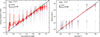 |
Fig. 6. Same as Fig. 5 but for the [M/H] and E(B-V) estimates (left and right panels, respectively). |
| In the text | |
|
Fig. 7. Summary of the metrics (from left to right, median bias, scatter, fraction of outliers, and Pearson coefficient) in bins of of ‘observed’ magnitude in the i-band (and average S/N in the narrow-band filters) for the age (green), metallicity (blue), and dust attenuation (red) predictions. The empty circles are the metrics obtained by means of SED-fitting (details in Sect. 5.1) on the i∼ 17 mag bin, highlighting the improved performance of the NN estimates. |
| In the text | |
|
Fig. 8. Left: Difference in the predicted metallicity versus age difference, colour-coded by dust attenuation. Middle: Difference in the predicted dust attenuation versus age difference, colour coded by metallicity. Right: Difference in the predicted dust attenuation versus metallicity difference, colour coded by age. Upper panels show galaxies with i < 20.5 mag, bottom panels galaxies with i < 17.0. The white lines show 1, 2, and 3σ contours. |
| In the text | |
|
Fig. 9. Difference between the predicted and the input parameters from top to bottom: log(Age), [M/H] and E(B-V) for the sample limited to i < 19.5, divided into different SSP synthetic photometry (from left to right: E-MILES, CB19, and XSL). The colour intensity corresponds to the ‘observed’ magnitude. Red points indicate the median values in bins, with red error bars showing the interquartile range (25th to 75th percentiles) of the distribution. |
| In the text | |
|
Fig. 10. Projection of the synthetic photometry and the real J-PAS photometry in the 2D parameter space obtained by UMAP dimensionality reduction algorithm. Black and gray data show the J-PAS APER_COR_3_0 and AUTO fluxes, respectively, while each panel shows the synthetic photometry for the three SSP libraries used in the training of the NN (E-MILES in orange, CB19 in green, and XSL in blue). While a single library does not fully cover the parameter space observed in real J-PAS data, the coverage is notably improved when the three libraries are combined together. |
| In the text | |
|
Fig. 11. Age (left, colour-coded by metallicity), metallicity (middle, colour-coded by age), and dust attenuation (right, colour-coded by age) NN predictions versus MUFFIT SED-fitting predictions from Díaz-García (in prep.) for a sample of observed J-PAS galaxies. |
| In the text | |
|
Fig. A.1. Comparison of the metrics (bias, scatter, fraction of outliers and Pearson (dashed line) and R2 (thick line) coefficients (from left to right) for different parameters (age, metallicity, and E(B-V) (top to bottom) as a function of galaxy i-band magnitude, obtained for different training strategies, as stated in the legend (details in Sect. 3). |
| In the text | |
|
Fig. B.1. Loss curves (loss function as a function of training epoch) for the train (blue) and validation (orange) samples for the age (left), metallicity (middle), and dust attenuation (right) NN models. |
| In the text | |
|
Fig. C.1. NN predictions for different CSP models -from top to bottom: 1 Gyr bursts, two 1 Gyr bursts, constant SFR (colours correspond to different flavours, as stated in the legend). Age, metallicity, and dust attenuation predictions are shown (left to right). The dashed lines show the light-weighted ages, metallicities, or E(B-V). The vertical dashed lines in the middle panel show the time when the second burst takes place. |
| In the text | |
|
Fig. D.1. Same as Fig. 5 and 6 but for the output obtained with CIGALE SED-fitting (see Sect.5.1 for details). |
| In the text | |
|
Fig. E.1. Projection of the synthetic photometry in the 2D parameters space obtained with UMAP dimensionality reduction algorithms, colour-coded by age (upper left), metallicity (upper right), dust attenuation (bottom left), and observed magnitude (bottom right). |
| In the text | |
Current usage metrics show cumulative count of Article Views (full-text article views including HTML views, PDF and ePub downloads, according to the available data) and Abstracts Views on Vision4Press platform.
Data correspond to usage on the plateform after 2015. The current usage metrics is available 48-96 hours after online publication and is updated daily on week days.
Initial download of the metrics may take a while.