| Issue |
A&A
Volume 705, January 2026
|
|
|---|---|---|
| Article Number | A227 | |
| Number of page(s) | 12 | |
| Section | Astrophysical processes | |
| DOI | https://doi.org/10.1051/0004-6361/202556590 | |
| Published online | 20 January 2026 | |
Broad-band modelling of the GRB 230812B afterglow: Implications for very-high-energy γ-ray detections with IACTs
1
Department of Astronomy, Astrophysics and Space Engineering Indian Institute of Technology Indore, Simrol Khandwa Road Indore 453552 Madhya Pradesh, India
2
Gran Sasso Science Institute Viale F. Crispi 7 L’Aquila (AQ) I-67100, Italy
3
INFN – Laboratori Nazionali del Gran Sasso L’Aquila (AQ) I-67100, Italy
4
INFN – Sezione di Padova I-35131 Padova, Italy
5
INAF – Osservatorio Astronomica di Brera Via E. Bianchi 46 I-23807 Merate (LC), Italy
6
INFN – Sezione di Trieste via Valerio 2 I-34127 Trieste, Italy
7
Centre for Radio Astronomy Techniques and Technologies, Department of Physics and Electronics, Rhodes University Makhanda 6139, South Africa
8
Astrophysical Sciences Division, Bhabha Atomic Research Centre Mumbai 400085, India
9
Indian Institute of Astrophysics, II Block Koramangala Bengaluru 560034, India
★ Corresponding authors: This email address is being protected from spambots. You need JavaScript enabled to view it.
; This email address is being protected from spambots. You need JavaScript enabled to view it.
Received:
24
July
2025
Accepted:
21
November
2025
Abstract
A significant fraction of the energy from the gamma-ray burst (GRB) jets, after powering the keV–MeV emission, forms an ultra-relativistic shock propagating into the circum-burst medium. The particles in the medium accelerate through the shock and produce the afterglow emission. Recently, a number of GRB afterglows were observed in TeV γ-rays by Cherenkov Telescopes. This new observational window provides access to the broad-band spectra of GRB afterglows, which contain rich information on the microphysics of relativistic shocks and the profile of the circum-burst medium. Since the transition from synchrotron to inverse Compton regime in afterglow spectra occurs between hard X-rays and the very-high-energy (VHE) γ-rays, it is necessary to have a detection in one of these bands to identify the two spectral components. The early afterglow data in hard X-rays, along with the GeV emission, could help to accurately constrain the spectral shape and capture the spectral turnover to distinguish the two components. We present a multi-wavelength spectral and temporal study, focussed on the keV-VHE domain, of GRB 230812B, one of the brightest GRBs detected by Fermi Gamma-ray Burst Monitor (Fermi/GBM). We also include the detection of a 72 GeV photon by Large Area Telescope (Fermi/LAT) during the early afterglow phase. Through detailed modelling of the emission within the afterglow external forward shock in a wind-like scenario, we predict the multi-wavelength afterglow observations from optical (up to approximately one day) to high-energy band. We emphasise the importance of following up poorly localised GRBs by demonstrating that even in cases without prompt localisation, such as GRB 230812B, it is possible to recover the emission using imaging atmospheric Cherenkov telescopes (IACTs) thanks to their relatively wide field of view. The low energy threshold of the Large-Sized Telescope is essential in discovering the VHE component at the much higher redshifts typical for long GRBs.
Key words: astroparticle physics / methods: observational / ISM: jets and outflows / galaxies: jets / gamma rays: ISM / gamma-ray burst: individual: GRB230812B
© The Authors 2026
 Open Access article, published by EDP Sciences, under the terms of the Creative Commons Attribution License (https://creativecommons.org/licenses/by/4.0), which permits unrestricted use, distribution, and reproduction in any medium, provided the original work is properly cited.
This article is published in open access under the Subscribe to Open model. This email address is being protected from spambots. You need JavaScript enabled to view it. to support open access publication.
1. Introduction
Gamma-ray bursts (GRBs) are fast (MeV) transients from ultra-relativistic jets produced after the collapse of massive stars or compact binary mergers. These jets are powered by a central engine, typically a newly formed black hole (Narayan et al. 2001) created in such cataclysmic events. The internal dissipation of energy (Rees & Meszaros 1994; Daigne & Mochkovitch 2000) within the jet gives rise to highly variable (0.1–1 s) radiation, in the keV–MeV range, observed as the prompt emission. The residual energy of the jet is then transferred to the circum-burst medium through the formation of a relativistic collisionless shock. The particles from the medium accelerate through the shock and emit non-thermal radiation, usually by synchrotron and self-synchrotron losses, resulting in a broad-band afterglow that spans from gamma rays (γ-rays) to radio waves (Mészáros & Rees 1997; Paczynski & Rhoads 1993; Sari et al. 1998).
Since the launch of Fermi Space Telescope, thousands of γ-ray bursts have been detected by the Gamma-ray Burst Monitor (Fermi/GBM; Meegan et al. 2009) in the energy range 8 keV–40 MeV. Around 10% of them have been captured by the Fermi Large Area Telescope (Fermi/LAT; Atwood et al. 2009) in 0.03–300 GeV (von Kienlin et al. 2020; Narayana Bhat et al. 2016); 2FGLC1. The afterglow emission observed by Fermi/LAT has been widely understood to originate from the external forward shock via synchrotron emission (Kumar & Barniol Duran 2010; Ghisellini et al. 2010; Nava et al. 2011). However, the GRBs detected at very-high-energy γ-rays (VHE; E > 100 GeV) are only a handful. The discovery of GRB 190114C (MAGIC Collaboration 2019) and GRB 180720B (Abdalla et al. 2019) has unequivocally proven, for the first time, that GRB afterglows can produce photons above 100 GeV. Subsequently, a near-by γ-ray burst at z = 0.078, GRB 190829A (H.E.S.S. Collaboration 2021) showed that VHE emission from GRBs can last for long timescales, up to several days. In addition, GRB 201015A and GRB 201216C were also established as TeV emitters (Suda et al. 2022; Abe et al. 2024), where the latter was the farthest VHE-detected GRB so far with a redshift of 1.1 (Abe et al. 2024). The detection of the GRBs starting from the trigger time using imaging atmospheric Cherenkov telescopes (IACTs) is challenging due to the communication of the trigger of a burst from a satellite (Fermi and/or Swift) to the IACTs and the slew-time (typically around 20–30 s) required to start the observation. In contrast, GRB 221009A, the brightest γ-ray burst of all time, has been observed since the time of the trigger by LHAASO (LHAASO Collaboration 2023) until 6 ks, thanks to the larger field of view (FoV) of the telescope detecting gamma-ray photons up to 10 TeV.
The broad-band GRB afterglow emission from radio to high-energy is typically attributed to synchrotron radiation from particles accelerated across the shock produced by the blast wave as it propagates into the medium (Sari et al. 1996, 1998; Granot et al. 1999; Panaitescu & Kumar 2001; Zhang et al. 2006). Several works have theoretically explored the presence of another emission component in GRB spectra arising from synchrotron self-Compton (SSC) scattering of afterglow photons from the electrons (Sari & Esin 2001; Papathanassiou & Meszaros 1996; Derishev & Piran 2021). The availability of rich afterglow data from X-rays to TeV has made it possible to explore advanced models, such as inhomogeneous magnetic fields in the shocks (Khangulyan et al. 2024), pair loading effects (Derishev & Piran 2016), or early inverse jet breaks (Derishev & Piran 2024). The detection of a second component has been claimed in TeV emissions from GRB190114C and GRB180720B as well (MAGIC Collaboration 2019; Abdalla et al. 2019). However, in the case of GRB190829A, there is ambiguity, since the joint spectra can be explained by a single-component emission, while other studies (Salafia et al. 2022) indicate that a two-component model is required.
The sub-MeV to GeV observations during the early afterglow are essential to mark the end of the first high-energy component and the rise of the second component, commonly modelled with SSC. However, capturing the sub-MeV emission from slowly varying transients is challenging, as MeV instruments are typically background dominated. Although Swift’s Burst Alert Telescope (Swift/BAT; Barthelmy 2000) is sensitive in the hard X-ray band up to 150 keV, it detects about a factor of three less GRBs per year as compared to Fermi/GBM. Hence, in the case of bright GRBs, Fermi/GBM data can be leveraged to extract the sub-MeV afterglow using the orbital background subtraction method (Fitzpatrick et al. 2011). Such an early afterglow has previously been detected and studied in the case of GRB 221009A by Banerjee et al. (2025).
Triggered on 18:58:12 UT, August 12, 2023 (T0), GRB 230812B, is one of the brightest γ-ray bursts detected by Fermi/GBM, with a fluence of 2.52 × 10⁻⁴ erg/cm2 (Roberts et al. 2023). The duration (T90) as recorded by Fermi/GBM is 3.26 s2. High photon flux from the burst caused pulse pileup in GBM detectors for ∼1 s (Roberts & Cleveland 2024). The burst has also been detected in Fermi/LAT from the onset of prompt (Scotton et al. 2023) up to about 1000 s. The highest energy photon, with an energy of 72 GeV, was detected by LAT at approximately 32 s after the trigger. Since Swift/BAT did not detect the prompt emission, the burst could only be broadly localised by Fermi/GBM in the initial phase. After a delay of ∼25 ks from the GBM trigger, the Swift X-ray Telescope (Swift/XRT; Burrows et al. 2000) detected the X-ray afterglow and precisely localised the burst at RA = 249.13°, Dec = +47.86° (J2000; Beardmore et al. 2023). Later on, the optical observations from several telescopes revealed the presence of a supernova (SN) associated with the burst (Kumar et al. 2023), thereby confirming the stellar collapse origin. The spectroscopic observations from GTC and NOT optical telescopes measured at the redshift of z = 0.36 (de Ugarte Postigo et al. 2023; de Ugarte Postigo 2023). Subsequently, the radio afterglow was first detected by Arcminute Microkelvin Imager Large-Array (AMI-LA) around two days post burst at 15.5 GHz with a flux 280 μJy (Rhodes et al. 2023). Around the same time (∼2.3 days), it was also followed up by Karl G. Jansky Very Large Array (VLA) at 6 Hz and 10 GHz, detecting a flux of 230 μJy and 196 μJy, respectively (Giarratana et al. 2023). However, in further observations from ∼17 days post-burst onward, the source was not detectable in the radio sky, and only upper limits were obtained by VLA (Chandra et al. 2023) and upgraded Giant Metrewave Radio Telescope (uGMRT; Mohnani et al. 2023).
The extreme brightness of the GRB 230812B and the discovery of the 72 GeV photon motivated us to perform a broad-band spectral study of the burst from prompt to afterglow phase. Our primary aim is to study the joint MeV–GeV emission in the early afterglow, along with the broad-band emission at later times, to infer the microphysical properties of the burst. This would also help in understanding the spectral component(s) giving rise to GeV emissions. Furthermore, we explore the possibility of VHE emission from the burst, detectable by existing facilities.
This paper is structured as follows. In Sect. 2, we describe the methodology adopted for the analysis of multi-wavelength data obtained from various telescopes. Section 3 describes the results of our spectral analysis. We report the detection of rare MeV afterglow. In Sect. 4, we describe the spectral and temporal modelling of the burst and discuss a possible strategy to effectively capture the VHE emissions from such GRBs. Finally, in Sect. 5, we summarise the complete evolution of the multi-wavelength spectra and the microphysics of the emission region.
2. Multi-wavelength data analysis
We performed a multi-wavelength analysis of GRB 230812B to study its spectral and temporal evolution from prompt to afterglow phase. We analysed the high-energy γ-ray (HE; 0.1 < E < 100 GeV) from Fermi/LAT, hard X-ray data from Fermi/GBM in 8 keV–40 MeV, late time X-ray data from Swift/XRT in 0.3–10 keV, and radio data in 1.4 GHz from uGMRT. The data in the optical r′ band has been collected from Hussenot-Desenonges et al. (2024). In the following sections, the multiwavelength data analysis methods (or data sources) are described in detail.
2.1. Fermi/GBM
We divided the prompt emission phase (T90) into three temporal bins: 0–0.4 s (bin-1), 1.4–2.0 s (bin-2), and 2.0–3.6 s (bin-3). Fermi/GBM data from 0.4–1.4 s are excluded to avoid pulse pile-up and dead-time effects caused by the high photon flux, as recommended by the Fermi/GBM team (Roberts & Cleveland 2024). The time interval following the end of T90, namely, 3.6–10.2 s (bin 4), potentially marks the transition from the prompt to the afterglow phase. The afterglow is divided into three temporal bins: 10.2–25 s (bin 5), 25–250 s (bin 6), and 251.9–647.2 s (bin 7).
2.1.1. Prompt emission
For the spectral analysis of prompt emission, we utilised Fermi/GBM time tagged events (TTE) data, publicly available through the HEASARC GBM-burst catalogue3. We rebinned the TTE data to a resolution of 64 ms by binbytime method using the binning module for unbinned data in Fermi/GBM data tools (Goldstein et al. 2022). To remove the bad time intervals (BTI) in our analysis, we ignored the time bins consisting of photons that arrive between 0.4–1.4 s (Roberts & Cleveland 2024). For background estimation, we selected intervals (−20, −5) and (50, 80) s with respect to the trigger time and fit it with a polynomial function in GBM data tools. We found that the background can be fitted reasonably well with the first-order polynomial. The model is then interpolated in the source region and the modelled background counts are estimated for further analysis.
Subsequently, the spectrum, background and response files were extracted. We fit the prompt emission spectra using HEASOFT XSPEC version: 12.15.0. We used four NaI detectors n0, n3, n6, n7 in energy range 8–900 keV and one BGO detector b0 with energy range 0.32–40 MeV for the analysis. The choice of NaI detectors is based on pointing angle with the source to be less than 60°. For BGO, we selected the detector with the minimum pointing angle. For the spectral fit of this dataset, we used Poisson-Gaussian statistics (pgstat4) in XSPEC (Arnaud 1996). The fit results are shown in Table 1.
Time-resolved spectral analysis of GRB 230812B using Fermi/GBM data.
2.1.2. Afterglow
To accurately estimate the background and detect faint MeV emission during the afterglow, we used the orbital background subtraction technique (Fitzpatrick et al. 2011), which takes advantage of the periodic observing geometry of the Fermi spacecraft. Calculating the average counts over the consecutive orbits bracketing the desired time can effectively estimate the background. We used the daily CSPEC data5 from the day of the GRB event to generate source and background files. We estimated the background over 30 orbits using the Fermi GBM Orbital Background Subtraction Tool6 (OSV;7 Fitzpatrick et al. 2011; De Santis 2024). We note that we also tested alternate background selections with averaging ±14 and ±16 orbits; see Table A.1. Since the time of interest lies outside the duration of the prompt emission, using the standard response files available in the Fermi/GBM catalogue is not suitable for the analysis and might introduce inaccuracies. To generate precise response matrices at the source location, for each detector of interest for each time bin, we used the official Fermi tool GBM Response Generator8 on the daily data of the γ-ray burst. After generating the spectrum, response, and background files, we fit the spectra for bin 5 and bin 6 using power-law function in XSPEC. We use the XSPEC model cflux*powerlaw in order to calculate the integrated flux from the fit. We froze the normalisation parameter of the powerlaw function to 1 since the model is now normalised by the integral flux. However, for bin 4, we tested the spectral fit against the models power law (PL), smoothly broken power law (SBPL), band, band+powerlaw, and broken power law (BPL). For the afterglow bins, the two NaI detectors, n6 and n7 for bin 5 and n6 and n3 for bin 6, were selected as they have low pointing angles with the source throughout the time of interest. We analysed the afterglow spectrum in energy range 40–400 keV, covering the most sensitive energy range of the NaI detectors (Fitzpatrick et al. 2011; von Kienlin et al. 2020; Paciesas et al. 2012; Meegan et al. 2009). For GRB 230812B, we did not find any excess over the background in the BGO detector in the entire energy range 0.4–40 MeV during the afterglow bins (bins 5 and 6). Due to the low photon count, we used the cash statistic (Cash 1979) as the fit statistic for our analysis.
2.2. Fermi/LAT
We performed an unbinned likelihood analysis of Fermi/LAT data for the γ-ray burst, starting from the Fermi/GBM trigger time and extending up to 1000 seconds post-trigger, in the energy range of 0.1–100 GeV, using the GTBURST9 software from Fermi Science Tools. We selected the region of interest covering 12° around the source location RA = 249.13°, Dec = +47.86° (J2000) given by Swift/XRT observations (Beardmore et al. 2023). We used the P8R3_TRANSIENT020 event class, which is suitable for transient-source analysis, and the corresponding instrument response functions. An isotropic particle background (‘isotr template’ in GTBURST), along with galactic and extragalactic high-energy components from the Fermi Fourth Catalogue (4FGL), with a fixed normalisation (‘template (fixed norm)’) was used. To ensure 5σ detection, a non-uniform time binning scheme has been adopted with a criterion of test-statistic (TS) > 25 to fit the power-law (‘powerlaw2’ using GTBURST) spectral model. For the time bin 250–647 s, we found the flux upper limits with a TS = 20. The time-resolved spectral analysis as presented in Table 2. A 72 GeV photon at ∼32.13 s has been detected (Scotton et al. 2023) with a 99.99% probability of association with the GRB as found by employing the gtsrcprob method in GTBURST.
Results of the Fermi/LAT unbinned likelihood analysis for GRB 230812B using a power-law model.
2.3. Swift/XRT
The X-ray afterglow of the γ-ray burst has been observed by Swift/XRT starting approximately 25 ks after the Fermi/GBM trigger. We obtained the source and background spectral files, as well as the redistribution matrix and ancillary response files, for the Swift/XRT data in the 0.3–10 keV energy range from the online Swift/XRT GRB spectrum repository (Evans et al. 2009). The spectra were extracted in photon counting mode for four time bins: (25.4–27.2 ks), (30.9–38.2 ks), (191.7–215.6 ks), and (407.8–1466 ks). We fit the XRT data for all four time bins simultaneously with an absorbed power-law model in XSPEC, using tbabs*ztbabs*cflux*powerlaw. The cflux is used to calculate the unabsorbed flux in the 0.3–10 keV energy range. The XSPEC models tbabs and ztbabs take into account the Tuebingen-Boulder ISM absorption in the Milky Way and the host galaxy, respectively. The hydrogen column density of the Milky-Way in the burst direction has been fixed to NH = 2.02 × 1020 cm−2 (Willingale et al. 2013). The hydrogen column density of the host galaxy at redshift z = 0.36, NH(z) was left as a free parameter for the fit, common among all the spectra.
2.4. Optical
The optical afterglow and the associated SN (SN2023pel) were monitored by several optical telescopes. We retrieved the r′-band optical data from Hussenot-Desenonges et al. (2024), which were compiled from the GCN Circulars archive. The data set includes observations from various optical telescopes provided in Table A2 in Hussenot-Desenonges et al. (2024). We fit the decaying part of the light curve, prior to the emergence of the SN, to model the temporal evolution of the afterglow (see Sect. 3.2 for details) until the emergence of the SN. While observations in other optical filters were available, they were excluded from temporal fitting, as our aim is to model the burst’s temporal behaviour and jet dynamics rather than performing a detailed spectroscopic analysis for a band in which the source was seen at the earliest time and has a high cadence of observation. However, the data from multiple filters were used to construct the spectral energy distribution (SED) around 30 ks, which was further used to test the spectral modelling (Fig. 4).
2.5. Radio
We analysed the uGMRT data obtained through our Director’s Discretionary Time (DDT) proposal (ddtC304; PI: Shraddha Mohnani). Three observations, each with a 2-hour time slot, were conducted on 17 September 2023 and 30 September 2023, using Band 5 (1050–1450 MHz), and on 1 October 2023 using Band 4 (550–850 MHz).
We processed the interferometric data using CAsa Pipeline-cum-Toolkit for Upgraded Giant Metrewave Radio Telescope data REduction (CAPTURE;10 Kale & Ishwara-Chandra 2021). CAPTURE follows the standard procedure for interferometric data reduction, which includes initial flagging of bad data, followed by delay, band-pass, flux, and complex gain calibration. The flux density scale was set using the Perley–Butler 2017 scale (Perley & Butler 2017). After the initial calibration stage, we manually inspected the data and flagged any remaining corrupted data using rFlag and TFcrop. We then performed an additional round of calibration. The derived calibration solutions were applied to the target source, and the data were subsequently split for self-calibration. Three rounds of phase-only self-calibration were carried out, using gain solutions derived from the target itself to correct for phase errors. The final imaging was performed using WSClean (Offringa et al. 2014). For the 17 September Band-5 observations, we achieved a root-mean-square (rms) noise level of approximately ∼14 μJy/beam. However, no significant emission was detected at the location of the target source. We reported our analysis results in NASA’s General Coordinates Network (GCN) circular (Mohnani et al. 2023). To improve sensitivity, we combined the Band-5 datasets from the observations conducted on 17 and 30 September 2023. However, no radio counterpart was detected in the combined image either. At Band 4, we reached an rms noise of ∼40 μJy/beam. However, no detection was noted in Band 4 either.
3. Results
3.1. Recovering the afterglow from keV to GeV
Given that GRB 230812B is exceptionally bright (with fluence of 2.52 × 10⁻⁴ erg/cm2), we modelled the Fermi/GBM background using OSV (see Sect. 2.1.2) and recovered the rare MeV afterglow emission. We calculated the significance of detection (signal-to-noise ratio, S/N) using formula given by Li & Ma (1983, see our Appendix A). We estimated the flux and the spectral parameters of the faint MeV afterglow emission in the energy band of 40–400 keV up to ∼650 s post-trigger. The spectra beyond T90 required PL spectral model except for bin 4 (3.6–10.0 s), where the spectrum preferred a BPL. The spectral peak for bin 4 is estimated to be 99.2 ± 3.1 keV. For bins 5 and 6, the spectra were fitted with a PL with indices around −2.3, providing a bound on the peak energy less than 40 keV. The spectra for different bins are presented in Fig. 1 and the corresponding spectral parameters are presented in Table 1. We note that for bin 7, the source is in the low-S/N regime (∼3σ) with a poorly constrained spectral index (−1.2 ± 0.4). Therefore, in addition, we computed the flux fixing the spectral index to −2, which resulted in a flux of (5.8 ± 2.0)×10−10 erg cm−2 s−1.
 |
Fig. 1. Temporal evolution of broad-band SED of GRB 230812B from Fermi/GBM (Table 1) and Fermi/LAT (Table 2) analysis. Panels (a)–(c): Prompt emission phase (bins 1–3). Panel (d): Prompt-to-afterglow transition (bin 4). Panels (e)–(f): Afterglow phase (bins 5–6). Forward-folded flux data points from the NaI and BGO detectors, as well as from LAT, are shown as filled circles. The green band depicts the best-fit model in keV-MeV band resultant from Fermi/GBM analysis (extended up to 100 GeV in bins 1–4). The blue butterflies show the power-law model fit on Fermi/LAT spectra in 0.1 − Emax. Overall SED evolution shows the emergence and evolution of the spectral components. |
The joint observation performed by Fermi/GBM and Fermi/LAT allowed us to cover a broad energy range from 8 keV up to 100 GeV (see Fig. 1) until 1 ks from the onset of the burst. During the prompt emission phase (until the end of T90; 3.6 s), the spectra observed with Fermi/GBM are best described by the Band function (Band et al. 1993), whereas the Fermi/LAT spectrum was fitted with a power-law model. The Fermi/LAT spectrum during the prompt emission is softer than −2 and can be identified as a tail of the Fermi/GBM spectrum extrapolated to GeV energies (see Fig. 1). In bins 3 and 4, the spectra in Fermi/LAT can be identified as an additional spectral component given the softer β (see Table 1) hinting at the emergence of a second component. In bin 4, Fermi/GBM spectra is better described with BPL11. We find that for the afterglow bins, the Fermi/GBM spectrum is best described with PL indices softer than 2.2 (in the range 2.2–2.5; see Table 1). However, Fermi/LAT shows a spectral hardening (see bin 6, Table 2) with a photon index of 1.75 ± 0.15.
3.2. Temporal evolution: LC fitting
To infer the temporal evolution of GRB 230812B, we fit the light curves from Fermi/GBM, Fermi/LAT, Swift/XRT and optical (r′-band) with a power-law model, F = F0 (t − T0)−Γt, as shown in Fig. 2. We used Bayesian inference to estimate the temporal decay index (Γt) and the normalisation factor (F0). To estimate the posterior distributions of these parameters, we used a Markov chain Monte Carlo (MCMC) using the emcee sampler (Foreman-Mackey et al. 2013). The likelihood function was defined by assuming Gaussian errors in the flux measurements, ![Mathematical equation: $ {\ln \mathcal{L} = -\frac{1}{2} \sum_{\mathrm{i}} \left[ \frac{(\mathrm{F}_{\mathrm{i}} - \mathrm{F}_{\mathrm{model,i}})^2}{\sigma_{\mathrm{i}}^2} + \ln(\sigma_{\mathrm{i}}^2) \right]} $](/articles/aa/full_html/2026/01/aa56590-25/aa56590-25-eq1.gif) , and the uniform priors for the parameters were used.
, and the uniform priors for the parameters were used.
Bin 4 was excluded from the GBM and LAT light curves when the temporal fit was performed due to its close proximity to the prompt emission phase. For the optical light curve, we restricted the fit to data prior to the emergence of the associated SN (31–251 ks).
We found that the indices of temporal decline are similar for the multi-wavelength light curves (in optical, X-rays and GeV energies) from ∼10 s onward extending up to about ∼106 s. The individual temporal decay indices of the afterglow light curves resulting from the fit are reported in Table 4. Notably, for LAT, XRT, and r′, the temporal decay indices are consistent within statistical uncertainties. However, the early afterglow (within 10 ks) observed with Fermi/GBM in 40–400 keV is slightly steeper. Moreover, the data do not suggest the presence of the jet-break in optical, X-ray and GeV energies.
4. Theoretical modelling and interpretation
A more general interpretation of the broad-band emission of GRB 230812B can be obtained by combining together the whole observational data as shown in the SEDs and in the light curves in Fig. 1 and Fig. 2. We interpret this broad-band emission in the context of the standard external forward shock afterglow scenario. In this model, the two radiation components are produced by synchrotron and SSC mechanisms and they can explain the multi-wavelength emission (Sari et al. 1998; Sari & Esin 2001; Nakar et al. 2009). The model used for the interpretation was presented in Miceli & Nava (2022). The jet dynamics follows the approach proposed in Nava et al. (2013) in the homogeneous shell approximation. As a result, the only free parameters assumed are the initial Bulk Lorentz factor, Γ0, and the afterglow kinetic energy, Ek. We assumed that constant fractions of the kinetic energy of the blastwave are transferred to electrons (ϵe) and to amplify the magnetic field (ϵB). The electrons swept up by the shocks are assumed to be accelerated into a power-law distribution dN/dγ ∝ γ−p, where p is the electron spectral index and γ is the electron Lorentz factor. For the circum-burst environment, we considered a wind-like scenario with density n = 3 × 1035 A★ R−s, with s = 2 and A★ being the density normalisation for wind-like environments (Chevalier & Li 2000; Panaitescu & Kumar 2000). The choice of the wind-like environment, instead of a constant-density environment, can be justified theoretically (Chevalier & Li 2000), observationally (Tiwari et al. 2025) and by the associated supernova detection (Agui Fernandez et al. 2023; Hussenot-Desenonges et al. 2024) which indicates that the GRB progenitor is likely a collapsing massive star. In addition, the combination of information coming from multi-wavelength light curves and SED provides evidence for a preference for a wind-like scenario, as detailed in Sect. 4.2.
4.1. Modelling of multi-wavelength light curves
The resulting predicted afterglow emission covering the whole multi-wavelength range from radio to VHE and the time intervals from 0.1 s up to 107 s is shown in Fig. 3. The values of the afterglow free parameters that best reproduce the observations are Ek = 8 × 1052 erg, Γ0 = 70, A★ = 0.2, ϵe = 0.1, ϵB = 5 × 10⁻⁵, and p = 2.2. The model suggests that afterglow emission starts to dominate in the GBM band from around 25 s, while LAT data seem to be consistent with afterglow even at earlier time, from ∼5–10 s, as also seen from the time-binned spectra in Fig. 1. The modelling is able to consistently reproduce both the Fermi/LAT and Fermi/GBM observational data collected starting from ∼25 s up to t < 103 s and the X-ray and optical data collected from ∼104 s up to ∼106 s. No evidence for jet breaks or other dominant components is present until t ∼106 s. For t ≳ 3 × 10⁵ s, the optical data are dominated by the emission due to the SN. Therefore, we added this contribution to the predicted optical afterglow. Radio data were collected at late times from ∼105 s up to ∼3 × 10⁶ s for different frequencies, from 1.26 GHz up to 75 GHz. We produced the predicted light curves for two reference frequencies (i.e. 1.26 GHz and 6 GHz). In this case, the model predictions display a significant discrepancy with the observational data points and upper limits by a factor of ∼10 even though the expected decay of radio flux in an optically thin regime from ∼105 s up to ∼106 s is reproduced. Overall, multi-wavelength data can provide important clues on the free parameter of the GRB afterglow model and on the break frequencies (self-absorption frequency, νsa, minimum frequency, νm, and cooling frequency, νc) of the synchrotron spectrum. Assuming that the emission is produced in slow cooling (νm < νc), the adopted scenario for late-time data requires a hard value of p (adopted here as 2.2) to reproduce the X-ray and optical time-evolution following also the analytical prescription of Granot & Sari (2002). The radio detections at 105 s, followed by the upper limits or marginal detections at 106 s, can be interpreted as the emission produced in an optically thin regime (νsa < νradio) with the minimum frequency, νm, crossing the radio band during this time interval. On the other hand, the Fermi/GBM and Fermi/LAT early-time data can be used to constrain the free parameters of the GRB dynamics. In particular, the afterglow kinetic energy, Ek, cannot be higher than 8 × 1052 erg. From Ek, it is possible to estimate the prompt efficiency, defined as ηγ = Eγ/(Eγ + Ek). Since Eγ = 8.7 × 1052, the value of Ek inferred from afterglow modelling implies a prompt efficiency: η ∼ 0.5. In an internal shocks model (Rees & Meszaros 1994), such a high level of efficiency can be explained only by invoking contrived conditions; for instance, as a considerable (≫10) contrast in the bulk Lorentz factors of the colliding shells and a large ϵe ≫ 0.1. If the jet is Poynting flux-dominated, such a high level of efficiency could be achieved more easily (Drenkhahn & Spruit 2002; Lyutikov & Blandford 2003; Giannios & Spruit 2005; Giannios 2008; Zhang & Yan 2011).
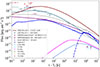 |
Fig. 3. Modelling of the multi-wavelength light curves with synchrotron and SSC scenario compared with early and late time afterglow observations for GRB 230812B. Predictions for the model are displayed in solid colored lines. The SN component is shown in dashed blue line. The corresponding instruments and energy bands are listed in the legend of the plot (see Sect. 2). |
Assuming the deceleration peak to be around 5–10 s when the afterglow component seems to start rising in Fermi/LAT spectra and light curves, we can derive acceptable values for Γ0 in the range between 70–100. Concerning the microphysical parameters, in the modelling, we adopted εe = 0.1 and εB = 5 × 10⁻⁵. These values are consistent with similar results obtained in modelling of GRBs detected in the HE and VHE domain (Gao et al. 2015; Gill & Granot 2022).
4.2. SED modelling
In Fig. 4, we compare the modelling discussed in the previous sections with the SED data at two different times. To cover the time evolution of the source, we considered two time intervals that are representative, respectively, of the early- and late-time emission (see Fig. 4): (i) the combined spectrum observed by Fermi/GBM (40–400 keV) and Fermi/LAT (0.1–100 GeV) in the 25–250 s time interval; and (ii) the late-time afterglow spectrum including optical and X-ray data at 30 ks.
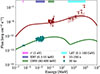 |
Fig. 4. GRB 230812B broad-band spectral energy distribution (solid red and green lines) modelling for two different time intervals, including early-time X-ray and high-energy afterglow data (25–250 s) and late-time afterglow optical and X-ray data at 30 ks. The afterglow emission is produced in the synchrotron and SSC external forward shock scenario. Observed data points (filled circles) and upper limits (arrows) from multiple instruments spanning the early to late afterglow phases are displayed. The energy bands used in the analysis are indicated in the legend: optical (r′; magenta), XRT (0.3–10 keV; purple), GBM (40–400 keV; green), and LAT (0.1–100 GeV; cyan). Details of the modelling and derived parameters are provided in Sect. 4. |
According to the model, the early-time Fermi/LAT emission is dominated by the SSC component of the spectra peaking in the GeV energy range and the Fermi/GBM emission is dominated by synchrotron emission in the limit just below the high-energy cutoff of the synchrotron spectrum and the rising of the SSC component. The minimum frequency, νm, is located in the optical band at a few eV, as also confirmed by the change of slopes in the predicted optical light curve at ∼250 s seen in Fig. 3.
The late-time optical and X-ray data at 30 ks are interpreted with the synchrotron spectrum in the slow-cooling scenario for frequencies, νm < ν < νc. We assumed a value of p = 2.2 which implies a Fν ∝ ν−0.6. The cooling frequency, νc, is found to be above the X-ray data (at around ∼50–100 keV) and the minimum frequency νm is at ∼0.5 THz (not visible in the plot). The behaviour shown in the late-time optical and X-ray spectrum justifies the preference for a wind-like environment. In fact, from optical to X-rays, observations at 30 ks are consistent with a single power-law spectrum rising in νFν, which can be explained assuming synchrotron emission in slow-cooling regime for frequencies νm < νopt < νX < νc. From the spectral analysis reported in Table 3, a photon index of ∼ − 1.65 was estimated from X-ray data at 30 ks. Considering theoretical prescriptions from Granot & Sari (2002), this implies a value of p ∼ 2.3, independently of the circum-burst environment. For a constant-density environment, this value of p implies a flux evolution ∝t−1, inconsistent with observations, as shown in Fig. 2, Fig. 3, and Table 4. On the other hand, a wind-like scenario implies a temporal evolution ∝t−1.47, which is in good agreement with the estimated X-ray and optical temporal indices and the SED and light curves modelling provided here.
Time-resolved spectral analysis results of x-ray afterglow of GRB 230812B from Swift/XRT in the 0.3–10 keV band.
Light-curve fitting results of GRB 230812B from various instruments.
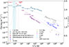 |
Fig. 2. Multi-wavelength flux light curve (left y-axis) of GRB 230812B obtained from Fermi/LAT (0.1–100 GeV), Fermi/GBM prompt (8 keV–40 MeV) and afterglow (40–400 keV), Swift/XRT (0.3–10 keV), and optical (r′) and radio (at various frequencies ranging from 1.2 to 75 GHz) telescopes. The GBM afterglow data is rescaled by a factor of 0.1 for plotting purposes. The faint data points correspond to fluxes obtained from finer time binning. The r′-band data show the optical afterglow and the emission from the associated SN. The solid lines corresponds to the best fit power-law model, F = F0(t − T0)−Γt for afterglow data from each instrument. For each instrument, the time interval used for the fit, along with the power-law index obtained as a result, is given in Table 4. The grey solid curve shows the count-rate light curve with rates depicted by the right y axis. |
4.3. Predicting VHE afterglow and detectability
The observation of a 72 GeV photon and the modelling of the LAT emission component in the 0.1–100 GeV energy range can be naturally interpreted with the presence of a SSC component in GRB 230812B. This result makes this event particularly interesting to test a possible detection in the tens-hundreds GeV energy band by IACTs. Unfortunately, none of the active ground-based instruments have reported the detection of the event. Nevertheless, rather than the intrinsic absence of a VHE component, this could be easily explained considering the low duty cycle of IACTs and the large localisation error of the event in the first minutes that impedes a rapid follow-up. We established an estimate of the expected intrinsic flux for two energies values, 25 GeV and 250 GeV, which are, respectively, representative of the lowest energy threshold for IACTs and of the typical energy value in standard VHE observations. We extracted the intrinsic flux at these energies and its time evolution using the same model inputs provided in Sect. 4. Then, we corrected the intrinsic fluxes for the attenuation due to the extragalactic background light (EBL) using the EBL model of Domínguez et al. (2011) to estimate the expected observed energy flux. We assumed two values for the redshift: the one estimated for GRB 230812B (z = 0.36) and a more distant redshift (z = 2), assuming the same intrinsic flux of GRB 230812B. The intrinsic and observed light curves for the two energy values are shown in Fig. 5 with different shades of red. We compared the expected VHE fluxes with the Cherenkov Telescope Array Observatory northern array differential sensitivities12 (CTAO-North) assuming three different exposure times (1 min, 10 min, and 60 min, shown in Fig. 5, marked in different shades of green) to explore the detectability of GRB 230812B by IACTs in the HE and VHE band.
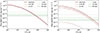 |
Fig. 5. CTAO-North array detectability of the predicted γ-ray emission at 25 GeV (left plot) and 250 GeV (right plot) for GRB 230812B (z = 0.36) and for a GRB 230812B-like event but with a larger redshift of z = 2. The red lines represent the intrinsic GRB emission (dark-red), EBL-attenuated (observed) emission at redshift z = 0.36 (red), and at redshift z = 2.0 (light-red). The horizontal lines are the differential sensitivity of CTAO with different exposures: 1 min: light-green, 10 min: green, and 60 min: dark-green. |
For the 25 GeV energy value, the flux in the early afterglow (within 1 ks) is above the sensitivity limit even considering a very low exposure of 1 min for the CTAO-North array and it extends up to ∼5 ks for an exposure of 10–60 min. In addition, the limited impact of the EBL at this energy is evident especially when considering the observed flux at redshift z = 2. As a result, larger distances did not significantly impact on the detection capabilities. For the 250 GeV energy value, results are slightly better for z = 0.36. The predicted flux is above the CTAO-North sensitivities for a 1 min exposure up to ∼1 ks and for 10 or 60 min exposures up to ∼10 ks. On the other hand, at redshift z = 2, the strong EBL absorption largely suppresses the flux which results to be more than one order of magnitude fainter than the differential sensitivities. These results (especially those obtained for the 1 min exposures) confirm that having the source in the FoV of CTAO-North array, even for a very limited time interval, which is compatible with a tiling strategy, could have resulted in a confirmed detection. However, relying on precise localisation is problematic. Indeed, the arc-second localisation of the burst, provided by Swift/XRT, was only available 30 ks after triggering, too late for effective GRB detection.
To understand the possibility of following up the GRB with IACTs, we explored the Healpix localisation maps13 through TilePy software (Seglar-Arroyo et al. 2024), an open-source Python package designed for the automatic scheduling of follow-up observations of transient events. Our estimates show that the GRB was visible to CTAO Large-Sized Telescope (CTAO/LST) for about one hour from the location of CTAO-North. In the following section, we show that even if the precise localisation was not known, a systematic tiling strategy might have resulted in a detection in VHE γ-rays.
We note that the first announcement of GRB 230812B (trigger number: 713559497)14 was communicated through GCN notices at Sat 12 Aug 2023 18:58:19 UT (T0; notice-1). The trigger was later updated by around 20 s, confirming that it originated from a GRB (T1: Sat 12 Aug 2023 18:58:42 UT) with probability of 96% (notice-2). In notice 2, within ∼20 s, the coordinate of the GRB was communicated with RA 248.867° and Dec +41.917° (L1) and with an associated error-radius of 3.22° (statistical only). In a follow-up notice (notice 3) within about 120 s (T2: Sat 12 Aug 2023 19:00:12 UT), a more precise localisation has been distributed with a revised RA 249.720° and Dec +45.970° (L2) with an error-radius of 1° (statistical only). This location is ∼1.9° away from the final localisation of the GRB as estimated by the XRT observations.
Since, the GRB was visible from the CTAO-North site, we propose a rapid follow-up strategy with CTAO/LST of the Fermi GBM localisation. We present this GRB as a hypothetical test case. Depending on the visibility in the sky (if the source is visible from the location of the CTAO), we propose slewing the telescope to the center of the error-region (in this case to L1) once the trigger is identified coming from a GRB (with probability of being a GRB to be more than 50%, usually announced in notice-2). The communication of the trigger and the slew time can reasonably be approximated to be around 60 s (circulation of the second notice: notice-2 and the reaction time of the telescope). This number includes around 30 s for the trigger communication and 30 s for the slew time. We propose performing a minute-long observation centred at L1 and initiating a tiling observation, as also generally proposed in searches for an electromagnetic counterpart of gravitational waves. The tiling should continue until the next notice (usually with a more precise localisation) arrives. In our case, the next notice (notice-3) arrives around 120 s from the trigger time. Hence, for this case, after a minute-long observation at L1, the telescope needs to be moved to L2, which might introduce a delay due to the slew rate of LST15. Once the telescope reaches the location, L2, we propose making a tiling of the 3σ error region, which in this case is 3° (1σ error region is 1°). The corresponding sky-localisation is about 28.3 deg2. Given the FoV of LST of 5 deg2, a total of about six points should be made in order to cover the sky-localisation patch. If 1 min is spent as an exposure (texp) for each tiling observation, the total time that is required to cover the 3σ error-region on notice-3 is about 360 s. A total latency of performing the observations proposed above is 510 s from the trigger time. We note from Fig. 5, in the left (right) panel, that the source at 25 GeV (250 GeV) is brighter than the limiting flux for a detection even beyond 510 s and could have been discovered with LST. Moreover, the source, if placed at a higher redshift, might have also been detected at lower energies (such as 25 GeV) since the spectrum was left nearly unaltered (see left panel of Fig. 5) by EBL absorption, as opposed to 250 GeV (see right panel of Fig. 5).
5. Discussion and conclusion
GRB 230812B is one of the brightest γ-ray bursts observed by Fermi/GBM, with a high fluence of 2.52 × 10⁻⁴ erg/cm2 (Roberts et al. 2023). Due to the large flux, the Fermi/GBM detectors experienced a pulse pileup for ∼1 s. GRB 230812B was detected by Fermi/LAT from the onset of the prompt emission and continued up to 1 ks extending well into the afterglow phase. Fermi/LAT recorded the highest-energy photon of 72 GeV at around 32 s after the trigger. Swift/XRT recorded the X-ray afterglow of the burst ∼25 ks post trigger (Beardmore et al. 2023). Subsequently, various optical telescopes monitored the burst and successfully detected the optical counterpart and the associated SN, SN 2023pel (Agui Fernandez et al. 2023). In the radio band, confirmed detections in the early days (< 17 days) and flux upper limits were obtained by later observations by AMI-LA (Rhodes et al. 2023), VLA (Giarratana et al. 2023; Chandra et al. 2023), and uGMRT (Mohnani et al. 2023) telescopes.
By collecting background photons from Fermi orbits with the same geographical footprints, preceding and following the observation of the γ-ray burst, we estimated the average background spectrum using the orbital subtraction tool (Fitzpatrick et al. 2011). We used custom response matrices generated for each time interval and were able to recover hard X-ray emission beyond T90. The hard X-ray spectra after 3.6 s were best described by a power-law model. The Fermi/GBM afterglow was extracted in the 40–400 keV energy band, which corresponds to the most sensitive range of the NaI detectors. In the absence of any detection with Swift/BAT, recovering the hard X-ray spectra with this method is pivotal because of the possibility of increasing the number of early-afterglow detections in GBM-detected GRBs.
The temporal index Γt of light curve during the afterglow (assuming F ∝(t − T0)−Γt seen in the energy band of 40–400 keV is 1.62 ± 0.13. The steeper temporal index might be a consequence of the inclusion of the temporal bin 10–25 s, which is close to the prompt emission phase and the prompt-contamination in this time bin cannot be ignored. We identified a similar temporal decline in X-rays (0.3–10 keV), optical (r′ band), and high-energy (0.1–100 GeV) γ-rays.
The combined Fermi/GBM and Fermi/LAT early-time (t < 103 s) data, taken together with the late-time (t > 103 s) X-ray, optical, and radio data, allowed us to build the broad-band light curves and SEDs and, hence, to model the afterglow emission and its time evolution over a wide range of frequencies. We used the numerical modelling presented in Miceli & Nava (2022) to derive the predicted time-evolving broad-band light curves of GRB 230812B from 0.1 s up to 107 s (see Fig. 3) and the SEDs for two selected time intervals (25–250 s; 30 ks, see Fig. 4) in the afterglow external forward shock scenario. We also added the prediction of the expected light curve in the VHE domain (0.1–5 TeV) for a typical energy range of observation. For the circum-burst environment, we adopted a wind-like scenario considering that the GRB progenitor is a collapsing massive star. The values of the afterglow free parameters that best reproduce the observations are Ek = 8 × 1052 erg, Γ0 = 70, A★ = 0.2, ϵe = 0.1, ϵB = 5 × 10⁻⁵, and p = 2.2.
Data collected from optical up to HE were consistently reproduced with the afterglow external forward shock scenario, without any evidence of jet breaks or other dominant components until ∼106 s; the only exception was the emission produced by the SN, which dominates optical data starting from ∼3 × 10⁵ s. Radio predictions from the modelling show a difference of a factor ∼10 with respect to the collected observational data points. Our modelling suggests that afterglow emission starts to dominate the GBM and LAT data, respectively, at ∼25 s and 5–10 s. In addition, GBM and LAT observations can be exploited to constrain the free parameters of the GRB dynamics; in particular, the afterglow kinetic energy, Ek, and the bulk Lorentz factor, Γ0. The time evolution of the X-ray and optical data provides evidence for a value of p = 2.2. The other microphysical parameters (εe and εB) are consistent with similar modellings of TeV-detected GRBs. From the SED modelling, we demonstrated that the sub-MeV afterglow emission detected by GBM arises from synchrotron radiation emitted just below the expected high-energy cut-off, while the LAT emission in the GeV domain is purely associated with the SSC component peaking in the GeV domain in the 25–250 s time interval. The late-time optical and X-ray data were consistently reproduced, assuming the synchrotron radiation in the slow cooling scenario (i.e. νm < ν < νc).
The detection of a 72 GeV photon offers compelling evidence to support the existence of a VHE emission component, as observed in a few GRBs to date. We estimated the expected intrinsic and EBL-corrected observed VHE light curves at 25 GeV and 250 GeV for GRB 230812B (z = 0.36) and for a simulated event with the same intrinsic flux as GRB 230812B, but assuming a higher redshift (z = 2). The choice of z = 2 is justified as the redshift distribution of long-GRBs peaks at around z = 2 (Ghirlanda & Salvaterra 2022; Palmerio & Daigne 2021). Then, we compared these light curves with the sensitivities of the CTAO-North array for a 5σ detection for the same energy values and assuming three different exposure times (1 min, 10 min, and 60 min; see Fig. 5). This comparison can provide a good proxy to evaluate whether future generation IACTs will be able to detect objects with similar VHE emission and until a specific time, with respect to the GRB trigger time. The emission at 25 GeV is chosen because it represents the energy threshold for the best observational conditions of IACTs. However, the emission at 250 GeV reproduces a more realistic observational condition for IACTs considering external factors (i.e. high zenith observations, high night sky background) that can easily degrade the energy threshold at the level of a few hundreds of GeV.
This comparison shows that early afterglow at 25 GeV and 250 GeV can be detected up to ∼1–10 ks with an exposure from 1 to a few tens of minutes. This calculation was performed based on the optimistic assumption that the GRB is localised and followed up from IACTs within the first tens or hundreds of seconds. It is of particular interest to note that the observed emission at 25 GeV is almost unaffected by the distance since the EBL impact is low at these energies. This is evident when considering the light curves obtained for the simulated event with the same intrinsic flux as GRB 230812B at redshift z = 2. In this case, while the expected observed flux at 250 GeV is always below the CTAO-North sensitivities, the expected observed flux at 25 GeV is above the sensitivities up to 1–10 ks. This indicates that future generation instruments like the LSTs or the CTAO-North array will be able to sensibly expand the horizon of detection of GRBs, exploiting their low energy threshold.
Given that the afterglow of GRB 230812B is estimated to be TeV-bright, the TeV detection depends on the early localisation due to the limited FoV of the IACTs (∼5–7 deg2). In this work, we propose the possibility of performing a systematic tiling to the localisation provided by the Fermi/GBM GCN notices distributed publicly right after the detection of the burst. The follow-up strategy should be made adaptive in such a way that the GCN notices received within a few minutes are followed up on and checked for a better sky localisation. Through simple estimates, we demonstrated that the GRB localisation might have been covered and a TeV component might also have been detected, based on the strategies mentioned above. However, the assumptions are rather simple and the development of more realistic estimates for time delays and tiling strategy is ongoing. This will be discussed in a future publication (Macera et al., in prep.). We summarise our conclusions as follows:
-
The emission mechanism in GRBs through the detection of multi-wavelength afterglow has been explored in detail thanks to GRB 230812B, primarily via its exceptional brightness and the visibility of the GRB (inside the Fermi FoV for both GBM and LAT) up to about 1000 s.
-
Although detections of the GeV emission in GRBs are common, due to the limited sensitivity in GeV band, it is challenging to establish the GeV emission to originate from the synchrotron and/or inverse Compton of the SSC model. We extracted the early afterglow emission by MeV detectors. By combining the sub-MeV and GeV early afterglow data, we constructed a multiwavelength spectrum. This spectrum was then reproduced with a synchrotron and SSC scenario.
-
We estimated the emission for gamma-rays in the lower energy band (25 GeV), which was achieved under optimistic observing conditions, and in the higher energy band (250 GeV), representing the threshold under realistic observing conditions. The early afterglow expected emission at 25 GeV is detectable with CTAO-North also up to redshift z = 2 until a few hours from the trigger time. The emission at hundreds of GeV is detectable for GRB 230812B until a few tens of minutes (103 s). However, intrinsic emission is highly attenuated at higher redshift (z = 2) even at energies around hundreds of GeV.
-
Although we state here that sub-TeV emission from GRB 230812B might have been potentially detectable by IACT, the main challenge is to design an optimal observational strategy. The TeV bright GRBs detected so far are triggered and localised by Swift/BAT. This is due to the availability of a precise position in the sky. Instead, the precise localisation of GRB 230812B was not available until 30 ks. We have demonstrated that optimising the observational strategy could enhance the probability of detecting GRBs with CTAO/LST. This involves promptly responding to early alerts from MeV detectors by targeting the initial, broader sky localisations provided in GCN notices. Tiling observations within the localisation region should be performed, with real-time updates as more precise localisations become available.
Acknowledgments
We acknowledge the use of data from the uGMRT for this study. We thank the staff of the uGMRT that made these observations possible. uGMRT is run by the National Centre for Radio Astrophysics of the Tata Institute of Fundamental Research. SM carried out a part of the research at GSSI, which was funded by the Fendi Prize money awarded to M. Branchesi. We thank Dr. V. Chitnis for valuable discussions and suggestions during the preparation of the uGMRT proposal. We also thank Dr. S. Mangla for their support in uGMRT data analysis. We thank the Department of Science and Technology (DST), India, for financial support under grant number CRG/2022/009332. This work made use of public Fermi-GBM and Fermi-LAT data and data supplied by the UK Swift Science Data Centre at the University of Leicester. BB and MB acknowledge financial support from the Italian Ministry of University and Research (MUR) for the PRIN grant METE under contract no. 2020KB33TP. DM acknowledges “funding by the European UnionNextGenerationEU” RFF M4C2 project IR0000012 CTA+. LN acknowledges funding by the European Union-Next Generation EU, PRIN 2022 RFF M4C21.1 (202298J7KT – PEACE).
References
- Abdalla, H., Adam, R., Aharonian, F., et al. 2019, Nature, 575, 464 [Google Scholar]
- Abe, H., Abe, S., Acciari, V. A., et al. 2024, MNRAS, 527, 5856 [Google Scholar]
- Agui Fernandez, J. F., de Ugarte Postigo, A., Thoene, C. C., et al. 2023, GCN, 34597, 1 [Google Scholar]
- Ajello, M., Arimoto, M., Axelsson, M., et al. 2019, ApJ, 878, 52 [NASA ADS] [CrossRef] [Google Scholar]
- Arnaud, K. A. 1996, in Astronomical Data Analysis Software and Systems V, eds. G. H. Jacoby, & J. Barnes, ASP Conf. Ser., 101, 17 [NASA ADS] [Google Scholar]
- Atwood, W. B., Abdo, A. A., Ackermann, M., et al. 2009, ApJ, 697, 1071 [CrossRef] [Google Scholar]
- Band, D., Matteson, J., Ford, L., et al. 1993, ApJ, 413, 281 [Google Scholar]
- Banerjee, B., Macera, S., De Santis, A. L., et al. 2025, A&A, 701, A68 [NASA ADS] [CrossRef] [EDP Sciences] [Google Scholar]
- Barthelmy, S. D. 2000, in X-Ray and Gamma-Ray Instrumentation for Astronomy XI, eds. K. A. Flanagan, & O. H. Siegmund, SPIE Conf. Ser., 4140, 50 [Google Scholar]
- Beardmore, A. P., Melandri, A., Sbarrato, T., et al. 2023, GCN, 34400, 1 [Google Scholar]
- Burrows, D. N., Hill, J. E., Nousek, J. A., et al. 2000, in X-Ray and Gamma-Ray Instrumentation for Astronomy XI, eds. K. A. Flanagan, & O. H. Siegmund, SPIE Conf. Ser., 4140, 64 [NASA ADS] [CrossRef] [Google Scholar]
- Cash, W. 1979, ApJ, 228, 939 [Google Scholar]
- Chandra, P., Ahumada, T., Bhalerao, V., et al. 2023, GCN, 34735, 1 [Google Scholar]
- Chevalier, R. A., & Li, Z.-Y. 2000, ApJ, 536, 195 [NASA ADS] [CrossRef] [Google Scholar]
- Daigne, F., & Mochkovitch, R. 2000, A&A, 358, 1157 [NASA ADS] [Google Scholar]
- De Santis, A. L. 2024, Orbital Subtraction Tool - GBM [Google Scholar]
- de Ugarte Postigo, A. 2023, GCN, 34410, 1 [Google Scholar]
- de Ugarte Postigo, A., Agui Fernandez, J. F., Thoene, C. C., & Izzo, L. 2023, GCN, 34409, 1 [Google Scholar]
- Derishev, E. V., & Piran, T. 2016, MNRAS, 460, 2036 [NASA ADS] [CrossRef] [Google Scholar]
- Derishev, E., & Piran, T. 2021, ApJ, 923, 135 [CrossRef] [Google Scholar]
- Derishev, E., & Piran, T. 2024, MNRAS, 530, 347 [NASA ADS] [CrossRef] [Google Scholar]
- Domínguez, A., Primack, J. R., Rosario, D. J., et al. 2011, MNRAS, 410, 2556 [Google Scholar]
- Drenkhahn, G., & Spruit, H. C. 2002, A&A, 391, 1141 [NASA ADS] [CrossRef] [EDP Sciences] [Google Scholar]
- Evans, P. A., Beardmore, A. P., Page, K. L., et al. 2009, MNRAS, 397, 1177 [Google Scholar]
- Fermi GBM Team. 2023, GCN, 34386, 1 [Google Scholar]
- Fitzpatrick, G., Connaughton, V., McBreen, S., & Tierney, D. 2011, Uncovering Low-Level Fermi/GBM Emission Using Orbital Background Subtraction [Google Scholar]
- Foreman-Mackey, D., Hogg, D. W., Lang, D., & Goodman, J. 2013, PASP, 125, 306 [Google Scholar]
- Frederiks, D., Lysenko, A., Ridnaia, A., et al. 2023a, GCN, 34403, 1 [Google Scholar]
- Frederiks, D., Lysenko, A., Ridnaia, A., et al. 2023b, GCN, 34414, 1 [Google Scholar]
- Gao, H., Wang, X.-G., Mészáros, P., & Zhang, B. 2015, ApJ, 810, 160 [NASA ADS] [CrossRef] [Google Scholar]
- Ghirlanda, G., & Salvaterra, R. 2022, ApJ, accepted [arXiv:2206.06390] [Google Scholar]
- Ghisellini, G., Ghirlanda, G., Nava, L., & Celotti, A. 2010, MNRAS, 403, 926 [NASA ADS] [CrossRef] [Google Scholar]
- Giannios, D. 2008, A&A, 480, 305 [NASA ADS] [CrossRef] [EDP Sciences] [Google Scholar]
- Giannios, D., & Spruit, H. C. 2005, A&A, 430, 1 [EDP Sciences] [Google Scholar]
- Giarratana, S., Giroletti, M., Ghirlanda, G., Di Lalla, N., & Omodei, N. 2023, GCN, 34552, 1 [Google Scholar]
- Gill, R., & Granot, J. 2022, Galaxies, 10, 74 [CrossRef] [Google Scholar]
- Goldstein, A., Cleveland, W. H., & Kocevski, D. 2022, Fermi GBM Data Tools: v1.1.1 [Google Scholar]
- Granot, J., & Sari, R. 2002, ApJ, 568, 820 [NASA ADS] [CrossRef] [Google Scholar]
- Granot, J., Piran, T., & Sari, R. 1999, ApJ, 513, 679 [NASA ADS] [CrossRef] [Google Scholar]
- H.E.S.S. Collaboration (Abdalla, H., et al.) 2021, Science, 372, 1081 [NASA ADS] [CrossRef] [Google Scholar]
- Hussenot-Desenonges, T., Wouters, T., Guessoum, N., et al. 2024, MNRAS, 530, 1 [NASA ADS] [CrossRef] [Google Scholar]
- Kale, R., & Ishwara-Chandra, C. H. 2021, Exp. Astron., 51, 95 [NASA ADS] [CrossRef] [Google Scholar]
- Khangulyan, D., Aharonian, F., & Taylor, A. M. 2024, ApJ, 966, 31 [Google Scholar]
- Kumar, P., & Barniol Duran, R. 2010, MNRAS, 409, 226 [NASA ADS] [CrossRef] [Google Scholar]
- Kumar, H., Swain, V., Teja, R., et al. 2023, GCN, 34500, 1 [Google Scholar]
- LHAASO Collaboration (Cao, Z., et al.) 2023, Science, 380, 1390 [NASA ADS] [CrossRef] [Google Scholar]
- Li, T. P., & Ma, Y. Q. 1983, ApJ, 272, 317 [CrossRef] [Google Scholar]
- Lyutikov, M., & Blandford, R. 2003, arXiv e-prints [arXiv:astro-ph/0312347] [Google Scholar]
- MAGIC Collaboration (Acciari, V. A., et al.) 2019, Nature, 575, 455 [Google Scholar]
- Meegan, C., Lichti, G., Bhat, P. N., et al. 2009, ApJ, 702, 791 [Google Scholar]
- Mészáros, P., & Rees, M. J. 1997, ApJ, 476, 232 [CrossRef] [Google Scholar]
- Miceli, D., & Nava, L. 2022, Galaxies, 10, 66 [NASA ADS] [CrossRef] [Google Scholar]
- Mohnani, S., Chatterjee, S., Banerjee, B., et al. 2023, GCN, 34727, 1 [Google Scholar]
- Nakar, E., Ando, S., & Sari, R. 2009, ApJ, 703, 675 [NASA ADS] [CrossRef] [Google Scholar]
- Narayan, R., Piran, T., & Kumar, P. 2001, ApJ, 557, 949 [NASA ADS] [CrossRef] [Google Scholar]
- Narayana Bhat, P., Meegan, C. A., von Kienlin, A., et al. 2016, ApJS, 223, 28 [NASA ADS] [CrossRef] [Google Scholar]
- Nava, L., Ghirlanda, G., Ghisellini, G., & Celotti, A. 2011, A&A, 530, A21 [NASA ADS] [CrossRef] [EDP Sciences] [Google Scholar]
- Nava, L., Sironi, L., Ghisellini, G., Celotti, A., & Ghirlanda, G. 2013, MNRAS, 433, 2107 [NASA ADS] [CrossRef] [Google Scholar]
- Offringa, A. R., McKinley, B., Hurley-Walker, et al. 2014, MNRAS, 444, 606 [NASA ADS] [CrossRef] [Google Scholar]
- Paciesas, W. S., Meegan, C. A., von Kienlin, A., et al. 2012, ApJS, 199, 18 [Google Scholar]
- Paczynski, B., & Rhoads, J. E. 1993, ApJ, 418, L5 [NASA ADS] [CrossRef] [Google Scholar]
- Palmerio, J. T., & Daigne, F. 2021, A&A, 649, A166 [NASA ADS] [CrossRef] [EDP Sciences] [Google Scholar]
- Panaitescu, A., & Kumar, P. 2000, ApJ, 543, 66 [Google Scholar]
- Panaitescu, A., & Kumar, P. 2001, ApJ, 560, L49 [NASA ADS] [CrossRef] [Google Scholar]
- Papathanassiou, H., & Meszaros, P. 1996, ApJ, 471, L91 [NASA ADS] [CrossRef] [Google Scholar]
- Perley, R. A., & Butler, B. J. 2017, ApJS, 230, 7 [NASA ADS] [CrossRef] [Google Scholar]
- Rees, M. J., & Meszaros, P. 1994, ApJ, 430, L93 [Google Scholar]
- Rhodes, L., Bright, J., Fender, R., Green, D., & Titterington, D. 2023, GCN, 34433, 1 [Google Scholar]
- Roberts, O. J., & Cleveland, W. 2024, GCN, 35660, 1 [Google Scholar]
- Roberts, O. J., Meegan, C., Lesage, S., Burns, E., & Dalessi, S. 2023, GCN, 34391, 1 [Google Scholar]
- Salafia, O. S., Ravasio, M. E., Yang, J., et al. 2022, ApJ, 931, L19 [NASA ADS] [CrossRef] [Google Scholar]
- Sari, R., & Esin, A. A. 2001, ApJ, 548, 787 [NASA ADS] [CrossRef] [Google Scholar]
- Sari, R., Narayan, R., & Piran, T. 1996, ApJ, 473, 204 [Google Scholar]
- Sari, R., Piran, T., & Narayan, R. 1998, ApJ, 497, L17 [Google Scholar]
- Scotton, L., Kocevski, D., Racusin, J., Omodei, N., & Fermi-LAT Collaboration. 2023, GCN, 34392, 1 [Google Scholar]
- Seglar-Arroyo, M., Ashkar, H., de Lavergne, M. d. B., & Schüssler, F. 2024, ApJS, 274, 1 [Google Scholar]
- Suda, Y., Artero, M., Asano, K., et al. 2022, in 37th International Cosmic Ray Conference, 797 [Google Scholar]
- Tiwari, P., Banerjee, B., Miceli, D., et al. 2025, A&A, submitted [arXiv:2510.05239] [Google Scholar]
- von Kienlin, A., Meegan, C. A., Paciesas, W. S., et al. 2020, ApJ, 893, 46 [Google Scholar]
- Wang, C.-Y., Yin, Y.-H. I., Zhang, B.-B., et al. 2025, ApJ, 980, 212 [Google Scholar]
- Willingale, R., Starling, R. L. C., Beardmore, A. P., Tanvir, N. R., & O’Brien, P. T. 2013, MNRAS, 431, 394 [Google Scholar]
- Zhang, B., & Yan, H. 2011, ApJ, 726, 90 [Google Scholar]
- Zhang, B., Fan, Y. Z., Dyks, J., et al. 2006, ApJ, 642, 354 [Google Scholar]
We tested the following models in search for the best fit model: PL, SBPL, Band, Band+PL, and BPL.
The Healpix maps contain the final localisation information of the GRB which is distributed as a final notice by Fermi/GBM of a burst (Fermi GBM Team 2023; https://heasarc.gsfc.nasa.gov/FTP/fermi/data/gbm/triggers/2023/bn230812790/quicklook/glg_healpix_all_bn230812790.fit).
Usually the slew rate is around 120° per 20 s. This rate implies that a slew of about 3° should take about a fraction of a second, which can be neglected.
Appendix A: Significance of detection of MeV afterglow
The detection of sub-MeV afterglow in Fermi/GBM (40-400 keV) heavily relies on the accurate modelling of the background. The OSV tool takes advantage of periodic orientation of the Fermi spacecraft. Fermi completes one orbit in 90 minutes and covers the full sky in every two orbits. The space craft reaches the orbital position at ± 24 hours or ± 15 orbits. Since the spacecraft also performs rocking maneuvers, the GBM detectors acquire the same pointing after ± 30 orbits. In our work we used ±30 orbits to extract the GBM background. However, we performed further tests to ensure that the source is detectable with alternate background considerations. Therefore, apart from ±30 orbits, reported in the results, we tested our analysis with alternate backgrounds with robust selection by averaging ± 14, ±16 orbits (Fitzpatrick et al. 2011). The significance of detection can be calculated formula given by Li & Ma (1983), expressed as
![Mathematical equation: $$ \begin{aligned} S = \sqrt{2} \, \Bigg \{ N_{\rm on} \ln \Bigg [ \frac{(1+\alpha )\, N_{\rm on}}{\alpha (N_{\rm on}+N_{\rm off})} \Bigg ] + N_{\rm off} \ln \Bigg [ \frac{(1+\alpha )\, N_{\rm off}}{N_{\rm on}+N_{\rm off}} \Bigg ] \Bigg \}^{1/2} ,\end{aligned} $$](/articles/aa/full_html/2026/01/aa56590-25/aa56590-25-eq2.gif) (A.1)
(A.1)
where Non represents number of photon counts from the source region and Noff is the number of photon counts from background region; α is the ratio of the on-source time to the off-source time. For constructing the GBM afterglow spectra, the on-source and off-source time is essentially the same, therefore, we used α = 1.
We calculated the significance of detection of the detectors used in spectral analysis for respective bins, due to a smaller angle with the source location. The results are compiled in Table A.1. For bin 5 and 6, the significance of detection for all the orbits stays well above 5σ. For bin 7, the detection significance is low (∼3σ for ±30 orbits and even lower for averaging ±14, ±16 case) resulting in upper limits, as in the case of LAT data for this bin. Moreover, the flux and indices obtained from these alternate background choices are consistent with the results reported in Table 1.
Significance of detection and best fit parameters for a power-law model of MeV afterglow.
Appendix B: Estimation of efficiency
The prompt efficiency of the burst is calculated using the ηγ = Eγ/(Eγ + Ek), where Ek denotes the kinetic energy of the blastwave and Eγ is the isotropic equivalent energy of the burst. Using the total gamma-ray fluence ℱγ recorded for the burst, Eγ can be calculated as  .
.
The redshift of GRB230812B is known to be  (de Ugarte Postigo et al. 2023). Various instruments have recorded its fluence across different energy bands, as detailed in Tab B.1. Based on these measurements, Eγ has been reported in the literature to lie within the range of 8.3 × 1052 to 1.11 × 1053 erg. In this work, we independently calculated Eγ from the fluence
  reported by Fermi/GBM (Roberts et al. 2023) in the energy range (10-1000 keV), adopting a flat ΛCDM cosmological model with parameters H0 = 67.7 km s−1 Mpc−1 and Ωm = 0.31. Our calculations result in the value of Eγ = 8.7 × 1052 erg, lying in close agreement with the values reported in literature (see Table B.1). From the modelling parameters that best produce the observational data, the kinetic energy of the blast wave is found to be 8 × 1052 erg. This results in efficiency of burst η ∼ 0.5.
Isotropic-equivalent energy (Eγ) and fluence from various instruments of GRB 230812B reported in literature from various instruments.
All Tables
Results of the Fermi/LAT unbinned likelihood analysis for GRB 230812B using a power-law model.
Time-resolved spectral analysis results of x-ray afterglow of GRB 230812B from Swift/XRT in the 0.3–10 keV band.
Significance of detection and best fit parameters for a power-law model of MeV afterglow.
Isotropic-equivalent energy (Eγ) and fluence from various instruments of GRB 230812B reported in literature from various instruments.
All Figures
|
Fig. 1. Temporal evolution of broad-band SED of GRB 230812B from Fermi/GBM (Table 1) and Fermi/LAT (Table 2) analysis. Panels (a)–(c): Prompt emission phase (bins 1–3). Panel (d): Prompt-to-afterglow transition (bin 4). Panels (e)–(f): Afterglow phase (bins 5–6). Forward-folded flux data points from the NaI and BGO detectors, as well as from LAT, are shown as filled circles. The green band depicts the best-fit model in keV-MeV band resultant from Fermi/GBM analysis (extended up to 100 GeV in bins 1–4). The blue butterflies show the power-law model fit on Fermi/LAT spectra in 0.1 − Emax. Overall SED evolution shows the emergence and evolution of the spectral components. |
| In the text | |
|
Fig. 3. Modelling of the multi-wavelength light curves with synchrotron and SSC scenario compared with early and late time afterglow observations for GRB 230812B. Predictions for the model are displayed in solid colored lines. The SN component is shown in dashed blue line. The corresponding instruments and energy bands are listed in the legend of the plot (see Sect. 2). |
| In the text | |
|
Fig. 4. GRB 230812B broad-band spectral energy distribution (solid red and green lines) modelling for two different time intervals, including early-time X-ray and high-energy afterglow data (25–250 s) and late-time afterglow optical and X-ray data at 30 ks. The afterglow emission is produced in the synchrotron and SSC external forward shock scenario. Observed data points (filled circles) and upper limits (arrows) from multiple instruments spanning the early to late afterglow phases are displayed. The energy bands used in the analysis are indicated in the legend: optical (r′; magenta), XRT (0.3–10 keV; purple), GBM (40–400 keV; green), and LAT (0.1–100 GeV; cyan). Details of the modelling and derived parameters are provided in Sect. 4. |
| In the text | |
|
Fig. 2. Multi-wavelength flux light curve (left y-axis) of GRB 230812B obtained from Fermi/LAT (0.1–100 GeV), Fermi/GBM prompt (8 keV–40 MeV) and afterglow (40–400 keV), Swift/XRT (0.3–10 keV), and optical (r′) and radio (at various frequencies ranging from 1.2 to 75 GHz) telescopes. The GBM afterglow data is rescaled by a factor of 0.1 for plotting purposes. The faint data points correspond to fluxes obtained from finer time binning. The r′-band data show the optical afterglow and the emission from the associated SN. The solid lines corresponds to the best fit power-law model, F = F0(t − T0)−Γt for afterglow data from each instrument. For each instrument, the time interval used for the fit, along with the power-law index obtained as a result, is given in Table 4. The grey solid curve shows the count-rate light curve with rates depicted by the right y axis. |
| In the text | |
|
Fig. 5. CTAO-North array detectability of the predicted γ-ray emission at 25 GeV (left plot) and 250 GeV (right plot) for GRB 230812B (z = 0.36) and for a GRB 230812B-like event but with a larger redshift of z = 2. The red lines represent the intrinsic GRB emission (dark-red), EBL-attenuated (observed) emission at redshift z = 0.36 (red), and at redshift z = 2.0 (light-red). The horizontal lines are the differential sensitivity of CTAO with different exposures: 1 min: light-green, 10 min: green, and 60 min: dark-green. |
| In the text | |
Current usage metrics show cumulative count of Article Views (full-text article views including HTML views, PDF and ePub downloads, according to the available data) and Abstracts Views on Vision4Press platform.
Data correspond to usage on the plateform after 2015. The current usage metrics is available 48-96 hours after online publication and is updated daily on week days.
Initial download of the metrics may take a while.