| Issue |
A&A
Volume 705, January 2026
|
|
|---|---|---|
| Article Number | A63 | |
| Number of page(s) | 16 | |
| Section | Interstellar and circumstellar matter | |
| DOI | https://doi.org/10.1051/0004-6361/202556774 | |
| Published online | 07 January 2026 | |
TRIShUL: Technique for Reconstructing magnetic Interstellar Structure Using starLight polarization
1
Institute of Astrophysics, Foundation for Research and Technology-Hellas,
Vasilika Vouton,
71110
Heraklion,
Greece
2
Department of Physics and Institute of Theoretical and Computational Physics, University of Crete,
Voutes Campus,
70013
Heraklion,
Greece
3
Université Libre de Bruxelles,
Science Faculty CP230,
1050
Brussels,
Belgium
★ Corresponding author: This email address is being protected from spambots. You need JavaScript enabled to view it.
Received:
7
August
2025
Accepted:
3
November
2025
Abstract
We present a novel technique for the decomposition of line-of-sight (LOS) stellar polarization as a function of distance, aimed at reconstructing 3D plane-of-sky magnetic structures in the interstellar medium. The method is based on the assumption that the observed polarization arises from discrete, thin dust layers located at varying distances along the LOS. Using a simple and intuitive frequentist framework, our method identifies structural changes in the distance-sorted cumulative Mahalanobis distance between Stokes parameters (q and u) to detect the locations of dust layers and estimates their associated physical properties (parallax and Stokes parameters) necessary for constructing 3D maps. We benchmarked the method using mock datasets representative of high-Galactic-latitude regions, incorporating realistic parallax uncertainties from Gaia and expected polarization measurements from the upcoming PASIPHAE survey. Our tests show that the method reliably recovers the distances and polarization properties of dust clouds when the polarization signal exceeds 0.1%, and the effective fraction of background stars is greater than 10% in our tested samples with ∼345 stars. The effect of background star fraction on the performance becomes less critical with increasing amplitude of the polarization source field from the dust cloud. We applied our method to existing polarization data from two illustrative sight lines - one at intermediate-high Galactic latitude and one near the Galactic plane - with known tomographic solutions, finding excellent agreement with the literature and demonstrating its accuracy across both regions. We compare the performance of our method with that of the Bayesian method BISP-1. While both methods effectively recover dust cloud properties, our approach is prior-free and computationally more efficient in determining the optimal number of clouds along the LOS. These advantages make our method more flexible and broadly applicable for multilayer dust cloud reconstruction for the upcoming era of large-scale stellar polarization surveys.
Key words: methods: statistical / techniques: polarimetric / dust, extinction / ISM: magnetic fields / ISM: structure
© The Authors 2026
 Open Access article, published by EDP Sciences, under the terms of the Creative Commons Attribution License (https://creativecommons.org/licenses/by/4.0), which permits unrestricted use, distribution, and reproduction in any medium, provided the original work is properly cited.
This article is published in open access under the Subscribe to Open model. This email address is being protected from spambots. You need JavaScript enabled to view it. to support open access publication.
1 Introduction
Our vantage point within the Galactic disk complicates the study of the global structure of the Galaxy, as multiple features are superimposed along each line of sight (LOS). Studies of the Milky Way interstellar medium (ISM) have traditionally relied on 2D sky projections (e.g., Schlegel et al. 1998; Planck Collaboration Int. XLVIII 2016; Lenz et al. 2017; Chiang 2023). However, recent advancements have enabled the exploration of the third spatial dimension: distance. The Gaia mission, with its precise parallax measurements of billions of stars (e.g., Gaia Collaboration 2018, 2023; Bailer-Jones et al. 2021), has been instrumental in this progress, allowing for detailed 3D mapping of the dust density in the ISM (e.g., Lallement et al. 2019, 2022; Green et al. 2019; Vergely et al. 2022; Edenhofer et al. 2024).
The enhanced resolution of 3D studies has provided new insights into local ISM structures, such as the Orion complex and other isolated molecular clouds (e.g., Doi et al. 2021; Rezaei Kh. et al. 2020; Tahani et al. 2022). These studies, as well as other methods independent of stellar distances (e.g., Tritsis & Tassis 2018), highlight the critical role of magnetic fields in shaping the morphology and formation of these regions.
Magnetic fields significantly influence the dynamics of the ISM at various scales (e.g., Pattle et al. 2023, and reference therein) and shape the large-scale structures of the disk and the halo of the Galaxy (e.g., Beck 2015; Clark & Hensley 2019). However, despite their importance, our 3D understanding of Galactic magnetic fields remains limited due to the lack of direct, spatially resolved measurements.
Various observational tracers, such as Zeeman splitting, Faraday rotation, synchrotron emission, and polarized thermal dust emission, have been utilized to study magnetic fields in the Galaxy. Each, however, has its own limitations: Zeeman splitting is very weak, and it is difficult to detect (Beck & Wielebinski 2013). Faraday rotation studies only probe the LOS information (e.g., Tahani et al. 2018; Dickey et al. 2022) and are sensitive to nearby small-scale structures (Wolleben et al. 2010). Our understanding of the magnetic field both in external galaxies and in the Milky Way has been greatly enhanced by observations of synchrotron and thermal dust emission. However, these tracers only provide plane-of-sky (POS) integrated information along the LOS, making it challenging to resolve 3D structures of the magnetic field where multiple dust clouds overlap. In addition, various magnetic field models (Sun et al. 2008; Jansson & Farrar 2012; Jaffe 2019; Unger & Farrar 2024; Korochkin et al. 2025), each with differing morphologies, fit equally well the polarized synchrotron, Faraday rotation, and dust emission (Planck Collaboration Int. XLVIII 2016). Therefore, integrated polarization data do not suffice to lift the existing degeneracies (Unger & Farrar 2024). For example, Pelgrims et al. (2025) showed that all fits of large-scale Galactic magnetic field could be biased by the presence of the Local Bubble.
On the other hand, starlight polarization, first observed by Hall (1949) and Hiltner (1949), offers a complementary probe. Aspherical dust grains align their short axes parallel to the ambient magnetic field. The background starlight, when it interacts with such grains, becomes partially linearly polarized due to dichroic extinction (Andersson et al. 2015). When combined with precise stellar distances from Gaia, starlight polarization enables a tomographic reconstruction of the POS component of the magnetic field, offering a unique opportunity to disentangle overlapping magnetic structures along the LOS (Panopoulou et al. 2019; Doi et al. 2021; Pelgrims et al. 2024; Angarita et al. 2025). The approach is uniquely feasible with only starlight polarization, as other magnetic field tracers lack the precise distance estimations necessary to separate the magnetic fields of different clouds along the LOS.
Recently, 3D tomographic maps of different regions of the Galaxy have been constructed using starlight polarization (e.g., Panopoulou et al. 2019; Doi et al. 2021; Pelgrims et al. 2023, 2024; Doi et al. 2024; Uppal et al. 2024; Angarita et al. 2025). Several regions of the sky have been mapped in linear polarization observations within the disk and in more diffuse regions (Clemens et al. 2012; Versteeg et al. 2023; Uppal et al. 2024; Pelgrims et al. 2024; Panopoulou et al. 2025). The upcoming PASIPHAE survey (Tassis et al. 2018) and the SOUTH POL survey (Magalhães et al. 2005) promise significant advancements by providing stellar polarization data for millions of stars covering a large area of the sky. In the upcoming era of large-scale polarization surveys, it is essential to develop algorithms that solve the inversion problem to unravel the intricate 3D structure of the magnetized ISM from starlight polarization data and stellar distances.
The first such automated framework is BISP-1 (Pelgrims et al. 2023), developed for the upcoming high-latitude polarization survey, PASIPHAE. It employs a Bayesian formalism for decomposing the starlight polarization with distance. Although originally designed for high-latitude regions, it has also been successfully applied to lines of sight in the Galactic plane (Uppal et al. 2024; Bijas et al. 2024; Angarita et al. 2025). The current implementation of BISP-1 can model up to five thin dust layers along the LOS, which is a valid assumption for high-latitude fields; however, in the Galactic plane, characterized by higher dust densities and more complex structures, this assumption may be limiting. Moreover, evaluating multiple models (e.g., one to five-layer configurations) requires exploring a high-dimensional parameter space, making the method computationally expensive (e.g., requires ∼1 hour to process one LOS on an Apple M1 chip with 16 GB RAM).
In this paper, we present a novel and independent non-Bayesian method, named TRIShUL, developed for starlight polarization tomography. This method works on a per-LOS basis. In Sect. 2, we describe our methodology and its key components designed to identify the optimal number of dust layers along the LOS. We also explain how the method estimates the average properties of each dust layer, such as parallax and Stokes parameters, along with their associated uncertainties. A rigorous testing for benchmarking the performance and identifying the limitations of our method in low polarization (≤1%) and low signal-to-noise (S/N) is presented in Sect. 3. In Sect. 4, we present a detailed performance comparison between our method and BISP-1 by applying both to mock datasets representing one-and two-layer sight lines. In Sect. 5, we applied our method to published stellar polarization observations, demonstrating its applicability to both high-latitude regions and fields near the Galactic plane. We finally summarize and conclude our work in Sect. 6.
2 Methodology: TRISHUL framework
Our method is based on the fact that starlight becomes partially polarized when it passes through the dust clouds present along the LOS. As a result, when an ensemble of stars at different distances along a LOS is analyzed, the presence of multiple dust layers can be inferred from sudden “jumps” in the polarization signal as a function of distance. To capture these features, our approach relies on the following assumptions.
First, we used stellar polarization measurements within a finite circular area centered on each LOS. The area was chosen to be small enough to avoid significant large-scale POS polarization variations caused by spatially varying dust structures and large-scale ISM turbulence, so that a meaningful mean polarization could be defined. The scatter in the relative Stokes parameters (q, u) reflects the contributions from small-scale inhomogeneities and observational noise. Second, we assumed that polarization is induced by a set of discrete, thin dust layers along the LOS. This assumption is justified in the low polarization regime, where each layer contributes independently to the total observed polarization and can be modeled as the vector sum of the Stokes parameters from all foreground layers (Appendix B of Patat et al. 2010). Third, we assumed that the observed polarization is entirely due to the intervening magnetized ISM, with no contribution from stellar intrinsic components such as circumstellar disks or asymmetric stellar envelopes (e.g., Cotton et al. 2016; Bailey et al. 2024).
Our method, named TRIShUL, draws inspiration from Indian mythology, where it means “trident”. The three prongs of the TRIShUL represent the three key steps in our approach, the details of which are discussed in the following subsections along with the post-processing steps for calculating the physical parameters associated with the identified layers.
2.1 Calculating cumulative Mahalanobis distance
Early efforts to decompose starlight polarization as a function of distance were initiated by Andersson & Potter (2005) and Pavel (2014). Traditional approaches to tomographic decomposition of the magnetized ISM often rely on detecting sudden changes or jumps in polarization as a function of stellar distance (e.g., Panopoulou et al. 2019; Doi et al. 2021, 2024; Uppal et al. 2024). An example of step changes in the polarization (Stokes parameters), when dust clouds uniformly polarize an ensemble of background stars, is shown in the top-left panel of Fig 1. However, in reality, various factors, including turbulence in the ISM, polarization S/N, fluctuations in dust density, and variations in polarization efficiency, collectively obscure the detection of these discrete jumps, making their identification challenging (similar to the top-right panel of Fig. 1).
Doi et al. (2024) employed the strucchange package in R (Zeileis et al. 2003) to detect structural changes in the Stokes parameters as a function of the stellar distance, enabling the estimation of dust cloud distances along the LOS. This approach is effective when observed polarization jumps are distinctly seen above the noise level. However, in low-polarization regimes, commonly observed at high Galactic latitudes, or in low polarization S/N, the accurate identification of such discrete jumps becomes significantly more difficult (for example, in the cases similar to Fig. 1, top-right panel). To address this, our method introduces a novel approach: we track changes in the slope of the cumulative Mahalanobis distance computed from the Stokes parameters of stars sorted by distance along LOS. The Maha-lanobis distance (dMaha) of Stokes parameters, St = [q, u] from point (0,0) on the polarization plane is given by
 (1)
(1)
where, Σ denotes the covariance matrix of q and u parameters of a star. For a set of N stars with individual Stokes parameters (qi, ui) along the LOS, the cumulative Mahalanobis distance up to the j-th star is computed as
 (2)
(2)
We made the following key choices in our method as compared to others found in the literature. We used Mahalanobis distance to represent the polarization signal for two primary reasons. First, it combines the information from both Stokes parameters (q and u) into a single statistically robust scalar, preserving sensitivity to variations in either component while avoiding the computational complexity of analyzing them separately. Second, and more importantly, unlike the degree of polarization, which is positively biased in the low S/N regime (Clarke 2010), the Mahalanobis distance provides an unbiased statistical measure by incorporating individual uncertainties and their covariance. This makes it a robust and reliable indicator of polarization changes along the LOS, especially when identifying subtle jumps caused by dust layers in noisy observational data.
Instead of using physical distances or parallaxes directly on the X-axis, we sorted stars by distance and used their indices as a proxy for the position of stars along the LOS. This choice avoids artifacts arising from the nonuniform spacing of stars in distance (or parallax space), which can influence the estimation of slope or trend changes in Mahalanobis distance profiles. In addition, distance itself is not a directly measured quantity (derived from parallax or photometry), hence, it involves model-dependent assumptions and uncertainties. Alternative representations, such as using distance modulus or parallax on the X-axis, may complicate interpretation due to their nonlinear relationship with physical distance. As part of our method development, we explored all these alternatives and found that using distance-sorted indices best serves our goal. This approach not only regularizes sampling along the LOS but also enables a more intuitive interpretation of cloud locations in terms of the relative number of stars located before and after a dust layer. The effect of the distance or parallax uncertainties on the distance sorted indices is discussed in Sect. 2.3.
To enhance the detectability of weak polarization jumps, particularly in noisy and low-polarization environments, we used the cumulative Mahalanobis distances rather than the direct values. The summation process acts as a low-pass filter, suppressing the high-frequency fluctuations arising from measurement errors and ISM turbulence, while amplifying the global trends associated with actual dust layers. This technique is widely used in signal processing of noisy data (e.g., Lombard & Koen 1993; Fridman 2010; Ward et al. 2022). In the cumulative framework of TRIShUL, the presence of a dust layer is reflected not as an abrupt jump (which may be difficult to identify in noisy data), but as a distinct change in the slope of the profile.
The effect of cumulative Mahalanobis distance with indices over a low polarization signal is illustrated in Fig. 1. We use a simulated dataset of starlight polarization with distance from a toy model introduced in Pelgrims et al. (2023). In the model, each layer along LOS acts as a polarizing screen, inducing a mean polarization and scatter about it, which reflects the effects from turbulence-induced magnetic fluctuations in the beam. The simulated data contain two dust layers at distances d = 350 pc and 900 pc along the LOS. A jump in the q, u, and Mahalanobis distance (dMaha) is seen at the location of the dust clouds in the top and middle-left panel of Fig. 1. The cumulative profile of this data shows a changing slope near the location of the dust clouds, as shown in the bottom-left panel of Fig. 1. Incorporating Gaussian noise and scatter in the data around the mean polarization (as seen in the right panels of Fig. 1) can make it challenging to directly identify the cloud from individual polarization measurements (top-right panel). However, the cumulative Mahalanobis profile (bottom-right panel) has a visible changing slope near the actual dust layers.
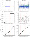 |
Fig. 1 Top left: q (in green) and u (in blue) as a function of distance-sorted stellar indices in a simulated LOS, without incorporating turbulence (internal scattering) and measurement uncertainties. Middle and bottom left: corresponding Mahalanobis distance (dMaha) and its cumulative effect ( |

2.2 Detecting breakpoints
The second key step of TRIShUL involves the automated detection of breakpoints in the distance-sorted cumulative Mahalanobis distance profile, i.e., positions along the X-axis where the slope changes significantly. For this, we applied statistical change-point detection techniques using the strucchange package in R (Zeileis et al. 2003). The cumulative Mahalanobis profile was modeled as piecewise linear functions of distance-sorted stellar indices, and strucchange identifies locations where regression parameters of these models change significantly. We controlled the analysis by specifying the minimum number of points per segment and the maximum number of breaks to test. The package implements the Bai & Perron (2002) methodology, which uses dynamic programming and performs several statistical tests to efficiently detect multiple structural changes. To prevent over-fitting, the optimal number of breaks (best-fit solution) was selected using the Bayesian information criterion (BIC), ensuring a balance between model complexity and goodness-of-fit (Schwarz 1978). The package also provides confidence intervals for each breakpoint, quantifying the associated statistical uncertainty. More details about the package can be found in Zeileis et al. (2002, 2003). An example of the application of the algorithm to the simulated data presented in Fig. 1 is shown in Fig. 2, both with (bottom) and without (top) measurement uncertainties, respectively. The bottom panel of Fig. 2 shows that the breakpoint detection algorithm (marked by blue lines) effectively recovers the locations of the true dust layers (shown in dashed red lines) from the cumulative Mahalanobis distance profile but also identifies spurious breaks. The false identifications likely arise from the accumulation of fluctuations (caused by both observational noise and ISM turbulence), which, when summed cumulatively, can mimic a genuine change of slope. To recover the correct number of dust clouds along the LOS, it is necessary to distinguish the true breaks from the spurious ones. This was done through a filtering procedure explained next, which forms the third and most critical aspect of our method.
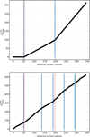 |
Fig. 2 Breakpoints (blue lines) detected in the distance-sorted cumulative Mahalanobis distance profiles using the R strucchange package. Top panel: results for mock data shown in the bottom-left panel of Fig. 1. Bottom panel: results for the mock data shown in the bottom-right panel of Fig. 1. The vertical dashed red lines indicate the input distances of the dust layers used in the simulations. |
2.3 Rejecting spurious breaks
Physically, a true dust layer should produce a significant change in the average Stokes parameters (q and u) across its location, whereas spurious breaks are expected to show statistically similar distributions of (q, u) on either side. To implement this, we split the data at each detected breakpoint into segments and apply a Hotelling’s T-squared test (Hotelling 1992) to compare the (q, u) distributions on either side, using the multivariate_ttest function from the Python Pingouin package (Vallat 2018). This test requires a minimum of five stars in each segment.
The standard implementation of the test does not incorporate measurement uncertainties in q and u parameters, which are critical in our case. We therefore reformulated the null hypothesis (i.e., the absence of a cloud) by modeling (q, u) pairs from both segments as a bivariate normal distribution, with the mean given by the inverse-covariance weighted average and the covariance by the unbiased weighted sample covariance of the combined data. Measurement noise was incorporated by performing Monte Carlo simulations, i.e., synthetic datasets for each segment were drawn from the estimated bivariate distribution, with both intrinsic dispersion and individual measurement uncertainties of each star added to the covariance of the distribution. The contribution of the intrinsic dispersion was estimated by subtracting the average contribution of measurement noise from the weighted covariance of the combined data. We reapplied Hotelling’s T2 test on each simulated segment under the null hypothesis to determine how frequently the test statistic exceeds the observed value. A break was considered statistically significant if fewer than a specific percentage (e.g., threshold = 1%) of the simulations produced a test statistic greater than the observed one. This threshold was left as a user-defined parameter, as it depends on the level of uncertainties in the polarization measurements.
Furthermore, in our approach, we only used the absolute distance information in defining the indices, without considering their uncertainties. Consequently, stars near the breakpoints may have been misassigned between the segments. These stars, which we refer to as “jumpers”, can potentially change the weighted mean q and u of the segments, leading to spurious detections of the cloud layers. To mitigate this effect, we removed stars within 3σ of the breakpoint in parallax space, provided they constituted no more than 10% of the stars in the corresponding segment. This criterion strikes a balance between removing potential jumpers and retaining a sufficient number of stars to assess the statistical significance of each layer. Hotelling’s T2 test was applied to this restricted sample to determine whether the break remained statistically significant under the null hypothesis.
We applied these tests iteratively to each identified break along the LOS, sequentially redefining the segments based on the acceptance and/or rejection of the previous break. In this dynamic procedure, the segments may vary depending on the direction of analysis, i.e., forward: proceeding from minimum to maximum distance or backward: from maximum to minimum. A true physical break is expected to show statistical significance regardless of the direction of analysis. Breakpoints that are statistically significant in only one direction were flagged as uncertain (flagged as “1”), indicating potential inconsistency and the need for further scrutiny of the polarization data or adjustment of the hyperparameters of the strucchange algorithm (see Appendix A for more details on the nature of flagged cases). Valid reconstructions, consistent in both directions, were flagged as “0” (valid).
2.4 Post-processing
The three-core steps of TRIShUL described above yield breakpoints in index space, along with associated ∼1σ confidence intervals. The next step involved translating these break positions (stellar indices) into physically meaningful parameters. This included estimating the average parallax (proxy for distance) and mean Stokes parameters (proxy of degree of polarization and polarization angle, which indicate the POS magnetic field orientation) of the identified clouds along with their associated credible intervals.
2.4.1 Parallax estimation
We mapped the confidence interval bounds from index space to parallax space by selecting the parallaxes of the stars corresponding to the lower and upper index bounds, rounded to the nearest integers using the floor and ceiling functions. The parallax of the star at the breakpoint index was taken as the representative of the distance of the dust layer, with its statistical uncertainty approximated as half the difference in parallaxes corresponding to the upper and lower bounds. Since the breakpoint method does not account for observational uncertainties in either polarization (q, u) or parallax, the uncertainties estimated above might be underestimated. To account for parallax measurement errors, we added in quadrature the median parallax uncertainty of stars within the confidence interval to the breakpoint-based parallax uncertainty.
In addition to the statistical uncertainties, we also accounted for potential systematic effects in the estimated break points. For this, we segmented the data around each statistically significant breakpoint. The left-side uncertainty was calculated using the weighted mean Stokes parameters (q, u) of the right-hand segment as a reference and incrementally included stars from the left segment away from the break, recalculating the mean at each step. The process was stopped when the difference from the reference exceeds 2σ in either q or u. The parallax of the last included star defines the left-side systematic boundary. We tested for 1σ, 2σ, and 3σ on the test samples discussed in Sect. 3 and found that 2σ reasonably aligns with the true location of the layers. The same procedure was applied in reverse to estimate the right-side boundary. These bounds provide a measure of systematic uncertainty in the location of the inferred dust layer.
To ensure that the identified dust layers are physically distinct, we retained only those layers that were separated by at least 2σ in parallax, where σ is the quadrature sum of the maximum (statistical or systematic) uncertainties on the right side of the foreground break and the left side of the subsequent one. Adjacent layers with separations below this threshold were merged together. The location of the merged layer was calculated as a weighted mean parallax, using inverse maximum uncertainties as weights. Left and right uncertainties were propagated separately to preserve asymmetry. We also updated the flagged status of the merged layer such that if both the original layers had a flag of “0” or “1”, the merged layer was assigned a flag of “0”; if one was flagged as “0” and the other as “1”, the flag of the merged layer was designated as “01”.
2.4.2 Estimating polarization properties
To estimate the average polarization properties of the identified clouds, we consider that the Stokes parameters of the stars in the background of multiple clouds result from the cumulative contributions from individual clouds. This approximation is valid for LOSs in diffuse ISM where the dust clouds act as weak polarizers (Patat et al. 2010). The Stokes parameters q and u for each dust layer were computed by subtracting the weighted average Stokes parameters of the stars in the foreground segment (preceding the cloud) from those in the background segment (following the cloud) around the dust cloud location. In defining these segments, stars whose parallax (distances) fall within the uncertainty range (systematic or statistical) of the position of the cloud layer were excluded to avoid contamination from “jumper” stars that may not be part of the defined segment. The weighted means of the Stokes parameters were computed using the full covariance matrix, ensuring proper error propagation. To report the uncertainties in the estimated q and u parameters of the layers, we used the error on the weighted mean.
2.5 Special treatment of the foreground dust layer
Observational data sometimes exhibit nonzero Stokes parameters (q, u) of the very first stars, indicating the presence of a dust layer foreground to the observed sample. Additionally, the breakpoint-detection algorithm may fail to identify a foreground break before which the mean q and u are expected to be statistically consistent with zero, primarily due to an insufficient number of nearby stars to assess the statistical significance of the first layer. To ensure that such early LOS polarization was not overlooked, we had to treat the foreground layer specially.
In our method, we included an optional correction step that assigns an upper limit to the location of a potential foreground dust layer. To estimate this upper limit, we searched for a foreground region in which the weighted average Stokes parameters q and u were consistent with zero within a 2σ confidence interval. This search was conducted starting from the location of the first cloud detected by the breakpoint algorithm and moving toward stars at lower distances, adding one star at a time. The index of the last star at which the accumulated group Stokes parameters became consistent with zero was designated as the boundary of the first dust layer. If no such boundary was found, we assigned the position of the first star as the upper limit on the cloud distance. The statistical upper limit on index-based uncertainty associated with this boundary was approximated using the next star beyond the identified index for the layer. These indexbased estimates were then mapped to parallax as discussed in Sect. 2.4.1. Nevertheless, only positive bounds (upper limits) should be reported in such cases. In this special case, the positive bounds indicate the positive uncertainties in the upper limit on the distance of the first layer.
3 Performance testing
The performance of the method was expected to be influenced by the amplitude of the polarization signal induced by the LOS cloud, the number of stars effectively sampling a given cloud, the S/N ratio of the polarization measurements, the degree of intrinsic scatter, and the number of clouds along a LOS. To test these effects, we used mock data representing typical one- and two-cloud LOS (hereafter 1-cloud and 2-cloud LOS, respectively) scenarios at intermediate and high Galactic latitudes that will be targeted in PASIPHAE. The polarization induced by the clouds to the background stars depends on polarization efficiency (maximum polarization induced to the stars per unit reddening), and apparent 3D orientation of the magnetic field (B) in the cloud, which is described by the inclination angle of magnetic field line with respect to POS (γBreg) and position angle of POS component of magnetic field (ψBreg) (Andersson et al. 2015; Hensley & Draine 2021). The mock data for benchmarking the method were generated using a toy model described in Pelgrims et al. (2023), where the total 3D magnetic field was modeled as a sum of regular (Breg) and stochastic component (Bsto) as Btot = Breg + Aturb Bsto. The parameter Aturb measures the amplitude of the stochastic component with respect to the regular one and takes care of the expected inhomogeneities in the polarization source field. Further details about the toy model and mock samples can be found in Sect. 4.1 and Appendices A3 and A4 of Pelgrims et al. (2023).
Our simulations assumed a 1° beam containing ~345 stars along the LOS. A fixed intrinsic scatter of Aturb = 0.2 was adopted, and we varied the distance(s) of the cloud layer(s) to vary the fraction of stars lying in the background of the cloud(s). For each configuration, we generated multiple realizations by varying the POS orientation of the regular magnetic field and the random seed of the stochastic magnetic field. These realizations formed the basis for testing our method to identify the number of clouds along the LOS and to recover their parallaxes and polarization properties. To interpret the results, we categorized the outcomes of our method into four categories: (i) false negative (FN), where no clouds were detected or a cloud was missed in two-cloud cases, indicating method failure; (ii) false positives (FP), where more clouds were identified than the number of clouds input to the mock data; (iii) Flagged or uncertain cases as discussed in Sects. 2.3 and 2.4.1; (iv) Valid reconstructions, where the number of identified clouds matches the input layers in mock data.
3.1 One cloud cases
In the single cloud setup, only one cloud was placed along the LOS. The distance of the layer was varied such that the fraction of stars located behind the cloud (fbg) was 90, 70, 50, 30, and 10% corresponding to the distances of approximately 270, 565, 790, 1050, and 1712 pc, respectively. The inclination of the regular component of the magnetic field with respect to the POS was fixed at γBreg = 0°. To test the performance of the method in the low polarization regime, we varied pmax from 0.05 to 0.3% with a step size of 0.05% and also considered higher values of 0.5, 0.75, and 1.0%. We further considered ten realizations of each pair of pmax and fbg, varying the POS position angle of Breg. All these combinations led to 450 simulated samples of starlight polarization data, where we applied our method to identify the number of clouds, estimate their parallax, and polarization properties.
We imposed a fixed minimum cut on the number of stars per segment to be five (set by Hotelling’s T2 statistical test). Each sample was tested for one to five layers and used the minimum BIC to find the optimal solution. The null hypothesis for statistically significant layers (see Sect. 2.3) was rejected at a 99% confidence level. Out of 450 simulated cases, our method successfully recovered the cloud layers in the majority of the cases. However, a subset of ~25% of cases results in FNs where no cloud layer was identified (case of failure). This does not imply a general failure of the method in 25% of cases; rather, these outcomes are closely linked to the effect of the degree of polarization induced by the cloud and the fraction of stars located behind it. Figure 3 shows the number of FNs as a function of the input degree of polarization (pmax) and the background star fraction (fbg). For pmax ≤ 0.1%, the polarization signal becomes too weak to be detected, leading to a higher FN rate. False negatives also extend toward the higher degree of polarization, but only when the background star fraction becomes as low as 10% (−34 stars). This is due to an insufficient number of background stars to confidently detect the slope change in the Mahalanobis distance.
Only −3% of the test samples resulted in FPs, where our method identifies two layers instead of one. In most of these cases, one layer corresponds to the true physical cloud, while the other shows polarization consistent with zero within 2σ. This suggests that the latter does not represent a physically distinct dust component and should not be treated as a separate cloud. These spurious layers can be removed, and the polarization properties of the remaining clouds should then be recalculated. In addition to FN and FP, only ~2% of the cases are classified as uncertain or flagged. These correspond to sight lines where at least one detected cloud is flagged due to ambiguity in the decomposition. Uncertain cases do not indicate a complete failure as the method still identifies dust layers, but these cases indicate that the LOS dust structure is complex or unclear, making the interpretation of the decomposition less straightforward. Therefore, the results from flagged sight lines should be used with caution (see Appendix A for more details). Heat maps illustrating FP and flagged cases, similar to the FNs, are shown in Appendix C. Unlike cases with FNs, these do not show any significant dependence on pmax or fbg. The remaining majority of the cases yield a single cloud with a flag of “0”, indicating a reliable and statistically significant result. These cases are summarized in the bottom panel of Fig. C.1.
To assess the accuracy of the calculated parallaxes and Stokes parameters of the valid identified dust layers, we avoided using the input values employed in generating the synthetic catalogs. Instead, we segmented the dataset at the input cloud distances and estimated the mean and covariance of the polarization signal attributed to the cloud by analyzing the Stokes parameters of stars located behind it. These values, referred to as the true polarization properties ( ), serve as an empirical benchmark. For parallax, we adopted the parallax of the star closest to the input cloud distance, denoted as ϖtrue.
We plot the differences between the estimated (est) and true values (true) of both parallax (top panel) and Stokes parameters (lower panels) for the identified cloud layers in Fig. 4. This figure illustrates the performance of the valid reconstructions across varying input degree of polarization (pinput on the X-axis), cloud distances (fbg, indicated by different colors), and polarization angles (number of points per pinput and fbg). In the top panel, the error bars on parallax represent the larger of the statistical or systematic uncertainties. The error bars in the bottom panel reflect the uncertainties in the estimated Stokes parameters, as described in Sect. 2.4.2. A horizontal offset of 0.02% is applied to each fbg group to prevent overlap of data points clustered around the same pinput values. The horizontal black line in the panels represents perfect agreement between estimated and true values. In the two panels, all data points seem to cluster around zero on the Y-axis, indicating strong agreement and high accuracy in the recovered values except at low polarizations, where deviations become more pronounced. The precision of the estimated parallax (top panel) deteriorates at fbg = 90% (purple points), as indicated by the larger uncertainties. This is due to the cumulative nature of the Mahalanobis distance we used in our method. With only ∼34 stars (10% of the stars) located in the foreground, the cumulative profile builds up slowly from nearzero values, causing a shift in the location of the detected slope change and leading to less precise parallax estimates. Nevertheless, in most cases, the discrepancies remain close to zero within the error bars. Overall, in 90% of the reliable cases, the estimated parallaxes agree with the true layer parallaxes within 2σ uncertainties. An opposite trend is observed in the lower panels for the q and u estimates, where low precision occurs at fbg = 10% (i.e., when only 10% of stars are present behind the cloud layer). This is also caused by low number statistics as the average q and u are derived from the background stars. A smaller sample size, especially with higher measurement uncertainties at the fainter end, compromises the precision of the weighted mean calculation. Nevertheless, the estimated q and u values agree with the true values within combined 2σ intervals in 99.5 and 90.5% of the cases, respectively.
We also investigated the effect of the inclination angle of the magnetic field with the POS on the performance of our method and find no observable trend. The detailed analysis is provided in Appendix B.
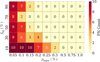 |
Fig. 3 Heat map illustrating the number of FNs out of 450 single-cloud mock samples, each with a combination of pinput and fbg, evaluated across ten samples of ψ ranging from 0° to 180°. The color intensity and the number within each cell represent the resulting count of FNs. |
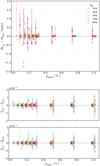 |
Fig. 4 Performance of TRIShUL as a function of input polarization signal for different cloud distances probed by fbg (in different colors). Top panel: difference between the estimated parallax (ϖest) and the parallax of the star closest to the input layer (ϖtrue). Bottom panel: difference in estimated Stokes parameters (qest, uest) from the corresponding true values (qtrue, utrue). The results corresponding to different fbg are shifted by 0.02% on the X-axis for visual clarity. Horizontal dashed lines are the references to a perfect match between estimated and true parameters. |
3.2 Two cloud cases
To test our method for cases with two clouds along the LOS, we used the samples described in Sect. 4.4 of Pelgrims et al. (2023). The first cloud was fixed at 350 pc, representative of the Local Bubble boundary at high Galactic latitude (e.g., Skalidis & Pelgrims 2019; Pelgrims et al. 2020). This distance corresponds to ∼55 stars located foreground the cloud for 1° beam-size (345 stars). The inclination angle of the magnetic field for the nearby cloud was fixed at 30°. Moreover, pmax was fixed, so that pc = 0.2%. The polarization angle for the nearby cloud was set at 22.5°. According to the discussion in Sect. 3.1, any cloud with such properties is expected to be well recovered by our method.
The performance of our method on two-cloud cases was expected to depend on the distance between the two layers, as they alter the number of foreground and background stars to the clouds, relative polarization amplitude, and possibly on the difference in the orientation of the magnetic field. Hence, the second cloud layer was added along the LOS with varying distance such that fbg2 = 90, 70, 50, 30, and 10%, meaning that this fraction of stars in the background of the nearby cloud were also in the background of the more distant cloud. The corresponding distances of the second cloud were approximately 520, 685, 900, 1150, 1800 pc, respectively. The polarization of the second cloud ( ) takes values of 0.05, 0.10, 0.15, 0.20, 0.25, 0.50, 0.75, and 1.00%, while the relative position angle of the magnetic field between the two clouds (∆ψ) ranges from 0° to 180° in steps of 30°. The inclination angle of the magnetic field of the second cloud was fixed to zero, and Aturb to 0.2. Five random realizations were used for each set, thus constructing 1200 simulated samples for the magnetized ISM structures along the LOS to test our method.
Similar to the one-cloud case, we applied our method to test one to five layers, keeping the minimum number of stars per segment fixed to five in the two-cloud scenario as well. Out of 1200 cases, only eight cases show complete failure in detecting both the clouds, while in 38% of the cases, only one of the two layers was identified. The combined statistics of FNs as a function of input parameters,  , ∆ψ, and fbg2 are shown in Fig. D.1 of Appendix D. Consistent with findings from the previous section, the results from two-cloud samples also demonstrate that clouds with low polarization signals (≤0.1%) or located at large distances (fbg2 = 10%) are more challenging to recover. The rate of failure is notably higher in the two-cloud scenario as compared to the single-cloud case, especially for fbg2 = 90%, i.e., when the two layers are close to each other. Accurate decomposition in the two-cloud configuration in these cases becomes particularly challenging because there are too few stars between the layers or an insufficient number of background stars behind the more distant cloud. In such cases, the algorithm often detected only one cloud, failing to resolve the second layer. For example, the cases when pc1 > pc2, the identified layer corresponds to the nearby one. However, as pc2 exceeds pc1, the decomposition results in the identification of the distant layer only. In 57% of the cases, we were able to identify both clouds, but ∼2% of these cases had one of the layers flagged as uncertain. In addition to FN and flagged cases, ∼4% of the reconstructions exhibit FP results. As discussed in the single-cloud case, the number of FPs and uncertain cases in the two-cloud case can also be decreased when layers with polarization consistent with zero are excluded.
For the valid reconstructions, excluding the flagged and FPs, the accuracy of our method in estimating both the parallax and polarization properties of the two clouds is illustrated in Fig. 5. The two panels at the top show the parallax accuracy for each layer, represented as the difference between estimated and true values. Different colors represent varying values of fbg2, following the same color scheme and offset as of fbg in Fig. 4. The data points in both the subpanels cluster closely around zero, indicating strong agreement between the estimated and true parallaxes. The upper subpanel (Layer 1) shows a larger number of points at low  compared to Layer 2 (bottom subpanel). This is primarily due to cases with FNs, where only the nearby cloud is detected for pc2 < pc1 as explained earlier. Even when both layers are detected, the estimated parallax of Layer 2 at low input polarization (
 ) deviates more than 3σ from the true value. This is because weak input signals make the second slope change harder to identify compared to Layer 1, where input-polarization is fixed at a relatively higher value (= 0.2%). Moreover, for low polarization, restricting the maximum number of breaks to five in identifying structural changes in Mahalanobis distance may be limiting, especially when multiple small variations arising from physical structure and the measurement noise have comparable amplitudes. In addition, the parallax estimates for Layer 1 show larger uncertainties and scatter compared to Layer 2. As explained in Sect. 3.1, the cumulative profile builds up gradually from near-zero values, making the first slope change harder to identify. Once the profile is established, subsequent layers exhibit a clearer slope change, leading to a more precise and accurate identification of Layer 2. The open black circles in Fig. 5 represent cases in which the algorithm correctly identifies the second cloud but detects a spurious, distant layer in place of the nearby one. These points are not associated with the nearby cloud but are shown to highlight false detections. Among the valid reconstructions, the estimated parallaxes match the true values within 2σ in 78% of the cases for the Layer 1 and 75% for the Layer 2.
The accuracy of the Stokes q and u parameters for the test samples is shown in the lower two panels of Fig. 5. Circular markers represent Layer 1 and square markers are used for Layer 2. To separate the visual representation of both layers, the left Y-axis corresponds to Layer 1 while the right Y-axis to Layer 2. The tight clustering of points around zero in both subpanels indicates good agreement between estimated and true values. The purple points (corresponding to fbg2 = 90%), however, show noticeably larger scatter and uncertainties, especially for Layer 1. This excess scatter is driven by cases with FNs where one of the two layers is missed, largely because only ~30 stars lie between the layers. Since the Stokes parameters q and u are derived after segmenting the data by identified cloud layers (as described in Sect. 2.4.1), missing a layer leads to incomplete decomposition and consequently biased polarization estimates. The blue points, corresponding to fbg2 = 10%, also exhibit larger uncertainties in the q and u differences, particularly for Layer 2. This is primarily due to the limited number of background stars behind the more distant cloud, which reduces the precision of the Stokes parameter estimates, similar to one cloud cases in Sect. 3.1. The plotted uncertainties represent the quadrature sum of the uncertainties in both the estimated and true Stokes parameters. In around 89% of the cases, the estimated q and u agree well with the true values within 2σ uncertainties.
It is worth noting that many of the cases where the estimated parallax and polarization properties deviate from the true values stem from inaccuracies in the locations of the breakpoints identified by the strucchange algorithm (see Appendix A for more details). When a true breakpoint corresponding to a cloud location is missed in the initial detection step, the error propagates through the subsequent analysis, ultimately causing departures from the true cloud properties. We used a maximum of five breakpoints in our current implementation for performance testing, and the final output was selected by optimizing solutions over one to five breaks. However, increasing the maximum number of breaks in strucchange could potentially improve the recovery of slope changes closer to the true locations of the clouds and thereby reduce the number of flagged cases, as well as enhance the precision and accuracy of the method. However, it may increase FP rates and also increase computational time, as more spurious breaks would need to be filtered out. Nevertheless, the current results are satisfactory, with most estimates lying within 3σ of the true parallax.
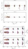 |
Fig. 5 Performance testing of our method in recovering parallax (top panel) and Stokes parameters (bottom panel) of both layers in two-cloud sample tests. The color scheme is defined for different sets of fbg2 and is similar to fbg in Fig. 4. The horizontal dashed lines correspond to a perfect match between the estimated and true values. The open black circles indicate cases where an additional, spurious layer beyond the second layer is identified, while the first layer is missed. Additional details about the figure are provided in the text in Sect. 3.2. |
4 Comparison with BISP-1
We compare the performance of TRIShUL with the LOS inversion method developed with a Bayesian framework (BISP-1) by Pelgrims et al. (2023). This method models between one and five thin dust layers along the LOS, each described by six parameters: (q, u, ϖ, Cq, Cu, Cqu). The algorithm employs the nested sampling implemented via dynesty code (Speagle 2020), where it uses the sampling points (called live points) to explore the parameter space and estimate the posterior distribution on model parameters. The results presented in Sect. 4.3 and Sect. 4.4 of their paper show the outcome of the BISP-1 algorithm using a one-layer model for single cloud samples and a two-layer model for two cloud samples. They also used prior information on cloud parallaxes to analyze the two cloud samples. For a fair comparison with TRIShUL, we reapplied the BISP-1 algorithm on mock samples, testing one to five-layer models, without imposing any external priors on cloud parallax. In our reanalyses, we used flat priors on Stokes parameters on q and u within ± 2%, and explored the parameter space by considering 1000 live points and sampling until we reached a total tolerance in the estimated log-evidence (check Eq. (15) of Pelgrims et al. 2023) below 0.1. All the pathological cases, where the parallax posterior peaked at the prior boundaries (indicating prior dominating solutions), were excluded, and the optimal model was selected using the minimum Akaike information criterion (AIC) (Akaike 1974). The AIC criterion measures the amount of information lost by representing the data with a given model.
For consistency, we allowed up to five layers in TRIShUL with a minimum of five stars per segment, and used 99% confidence level to reject the null hypothesis for valid breakpoints. We limit our comparison to one set of single- and two-layer cases in the low-polarization regime from Sect. 4.5 of the BISP-1 paper.
4.1 Comparison of one-cloud mock sample
We consider the mock LOSs containing a single dust cloud located at 350 pc, having a polarization of  , a magnetic field inclination angle of γBreg = 30°, and an intrinsic scatter Aturb = 0.2. The POS position angle of the magnetic field was varied from 0° to 162° in increments of 18°, and for each configuration, we generated ten random realizations, resulting in a total of 100 samples. Among the 100 samples, TRIShUL consistently identified a single layer, with two FPs but no FNs, and one reconstruction was flagged as uncertain.
For BISP-1, we adopted the default prior on parallax set by the five-layer model and inspected the resulting posteriors across all models. In nearly all cases, BISP-1 favored a one-layer model, with only two exceptions where a two-layer model is preferred based on AIC. However, we note that for these two cases, the probability that the one-layer model minimizes the loss of information based on the models’ AIC is above 30%. Therefore, the one-layer model cannot be rejected, and we treat these cases as equivalent to uncertain or flagged cases of TRIShUL.
To compare the accuracy of the two methods, we excluded reconstructions with FPs and flagged cases. Figure 6 presents a comparison of the retrieved parallaxes of the LOS cloud from both methods. We plot the mode of the posterior parallax for BISP-1 with its 16th and 84th percentile as asymmetric uncertainties on the Y-axis, against the estimate of TRIShUL on the X-axis. Uncertainties in estimates from TRIShUL are defined by the larger of the statistical and systematic errors on each side. To visualize the deviation of the estimated values from the true parallax, horizontal and vertical blue lines are plotted in the figure. In most cases, both methods yield parallax estimates that are systematically lower than the true values. This is due to the low number of stars in the foreground of the layer, as explained in Sects. 3.1 and 3.2. It is evident from the figure that the uncertainty estimates in TRIShUL are larger than those of BISP-1. Due to larger uncertainties, TRIShUL captures the true value within 1σ in 73% of the cases, while BISP-1 achieves ∼31% coverage. At the 2σ level, the coverage improves to 84% for TRIShUL and 97% for BISP-1. This indicates that TRIShUL provides results with lower precision than BISP-1.
The polarization properties of the clouds were computed based on both the true cloud layers and those identified by TRIShUL as described in Sect. 2.4.2. These are shown in blue and red points, respectively, in the bottom panel of Fig. 6. For comparison, the BISP-1 results are overplotted as black points, representing the mean Stokes parameters and their standard deviations from the posterior distributions. The estimates from TRIShUL and BISP-1 both closely align with the true values in almost all reconstructions, with only a few exceptions. These findings demonstrate that both methods yield accurate estimates of polarization properties for the single-layer mock datasets.
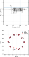 |
Fig. 6 Comparison of estimated parameters from BISP-1 (black) and TRIShUL (red) with the true values (blue) for parallax (top panel) and Stokes parameters (bottom panel) in one-cloud mock catalogs. |
4.2 Comparison of two-cloud mock samples
In this section, we consider the cases when two clouds are introduced along the LOS from Sect. 4.5.2 of Pelgrims et al. (2023). The nearby cloud was fixed at 350 pc with polarization degree of 0.2%, magnetic-field position angle ψBreg = 22.5°, inclination γBreg = 30°, and Aturb = 0.2. A second cloud was added at 685 pc (fbg2 = 70%), with a degree of polarization set to 0.2%, and an inclination angle of the magnetic field to 0°. The relative position angle of the magnetic field between the two clouds (∆ψ) was varied in the range 0° to 150° in steps of 30°. For each configuration, ten random realizations were generated, yielding 60 mock samples in total.
As reported in Sect. 4.5.2 of BISP-1, the analysis yielded 44 non-pathological parallax posterior distributions out of 60 mock samples, with the AIC favoring a two-layer model in 43 of these 44 cases. However, this result was achieved by imposing informative priors on cloud distances, i.e., assuming the presence of a nearby cloud within 100-600 pc and a second, more distant cloud within 300-3500 pc, and comparing the best AIC between one- and two-layer models only.
We reanalyzed two-cloud mock samples with BISP-1 without considering any external prior on parallax and updated parallax priors for all the models to priors informed by the five-layer configuration, instead of relying on the differing default priors typically associated with each model for a consistent comparison across models1. Out of 60 samples, 13 favor the one-layer model more than the two-layer model, thus constituting FNs. The remaining 47 cases led to a two-layer model as the best fit to the sample data.
In contrast, TRIShUL requires no prior information about cloud distances and performs robustly on the same two-cloud mock samples, yielding only two FNs and no FPs. Two additional cases were flagged as uncertain. Overall, the comparative statistics between the two methods highlights the effectiveness of TRIShUL in identifying the number of clouds along the LOS, without relying on prior knowledge of cloud distance.
The accuracy of the two methods in recovering the parallax and polarization properties of the identified clouds is illustrated in the top and bottom panels of Fig. 7, respectively. In both panels, the results from TRIShUL are shown in red, while BISP-1 outputs are represented by black markers. For the comparison of estimated parallax with the true values, the parallax based on input cloud distances is highlighted as a blue line in the top panel. Similarly, in the bottom panel, the true Stokes parameters, extracted by segmenting the data from the input distances, are shown in blue points along with the weighted error on the means. Flagged cases from TRIShUL are indicated by open blue circles in both panels. While the FNs of BISP-1 are marked by open black squares.
The top panel displays the estimated parallaxes from both methods for each LOS, sorted by ten random samples per difference in position angle of the two clouds as sample ID. In most cases, the black points lie closer to the blue line with smaller error bars, indicating that BISP-1 yields higher accuracy and precision compared to TRIShUL, which shows greater scatter and larger uncertainties. Despite this, most of our results remain within 3σ of the true values, indicating good accuracy but a lower precision. The precision of TRIShUL could be improved by relaxing the cap of five maximum breaks in breakpoint detection. Moreover, it is worth noting that TRIShUL successfully and accurately resolves sight lines that BISP-1 fails to identify, particularly for sample IDs between 30 and 40, which correspond to a specific configuration where ∆ψ = 90°.
Similar to parallax, the Stokes parameters estimated from both methods, represented in the bottom panel, generally agree with the true values within uncertainties. Excluding the flagged cases (indicated by open blue circles), TRIShUL closely recovers the true polarization in most cases, with only a few exceptions. BISP-1 also recovers Stokes parameters consistently across most cases. False negative cases show significant deviation from the true estimates (marked by open black squares in Fig. 7), which arise because the estimates are based on a single layer along the LOS rather than two.
In terms of computational efficiency, TRIShUL completes the tomographic decomposition of a typical LOS within only ∼2 minutes when testing up to five layers, whereas BISP-1 requires approximately 70 minutes to test all five models for the same LOS on the same machine (Apple MacBook Air with M1 chip, eight-core CPU, 16 GB RAM). Employing parallel processing for the null-hypothesis testing by distributing random draws for Monte Carlo simulations across multiple cores further reduces the runtime of TRIShUL by nearly half, with the same set of criteria as mentioned above. These advantages make TRIShUL computationally efficient and a broadly applicable method for multilayer dust cloud reconstruction.
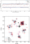 |
Fig. 7 Comparison of the estimated parameters from BISP-1 (black points) and TRIShUL (red points) with the true value (blue points) for parallax (top panel) and the Stokes parameters (bottom panel) of mock catalogs with two clouds. The open dark-blue circles indicate the flagged cases in TRIShUL and open black squares correspond to FNs in BISP-1. |
5 Application to observational data
In this section, we demonstrate the applicability of our method to real stellar polarization data. To assess its reliability across diverse ISM environments, we applied our method to two contrasting Galactic regions: (i) toward the Galactic plane, where the ISM is dense; and (ii) toward high Galactic latitudes, where the ISM is more diffuse and exhibits lower polarization.
Intrinsically polarized stars were expected to show a higher degree of polarization than neighboring stars and unrelated polarization angles. Such stars had to be removed from the data before applying our method for LOS tomography as mentioned in Sect. 2.
5.1 Toward high Galactic latitudes
We applied TRIShUL to R-band stellar polarization data from the high Galactic latitude regions centered around (l, b) = (104°.08,22°.31) and (103°.90,21°.97). The polarization dataset was obtained from Panopoulou et al. (2019) and consists of ∼100 stars toward both regions. The former sight line indicates the presence of at least 2-cloud, while the latter indicates only a 1-cloud along the LOS based on HI spectra.
Pelgrims et al. (2023) applied BISP-1 to these LOSs and successfully identified a single-layer structure along the 1-cloud LOS. However, toward the 2-cloud LOS, their analysis favored a one-layer model as the most probable rather than a two-layer model. They noted that while the one-layer model was preferred, their results did not entirely rule out the possibility of a second layer along that LOS. They found that, among the tested models, the two-layer model shows a probability of about 42% to be the model that actually minimizes the loss of information.
We applied TRIShUL to both datasets by setting the minimum number of stars per segment fixed to five, and no constraints on the maximum number of breakpoints. The spurious breaks were subsequently rejected to isolate statistically significant cloud layers with null-hypothesis testing at 99% confidence level. Our approach robustly identified a single polarization layer in the 1-cloud LOS (see top panel of Fig. 8). In contrast to BISP-1 results, our method successfully detected two distinct layers toward the 2-cloud LOS shown in the bottom panel of Fig. 8. The estimated distances of the identified layers in both regions agree with those reported by (GP19, Panopoulou et al. 2019) and (VP23, Pelgrims et al. 2023) within 2σ uncertainties, as shown by the orange and black lines in the plot marking the distance ranges labeled GP19 and VP23, respectively. We computed the polarization properties of the identified layers in both regions and compared them with the literature values in Table 1. The values derived from our method closely match the literature within the 1σ uncertainty level.
 |
Fig. 8 LOS decomposition of starlight polarization by TRIShUL displayed in (q, u) − μ (q in green, u in blue) plane for the polarization data from Panopoulou et al. (2019). The vertical lines indicate the positions of the cloud layers estimated by our method, with the shaded regions representing statistical (pink) and systematic (gray) uncertainties. Top panel: one-cloud region. Bottom panel: two-cloud region. The estimated distance range from Panopoulou et al. (2019) and Pelgrims et al. (2023) are marked in orange and black as GP19 and VP23, respectively. |
Comparison of polarization properties of clouds estimated from our method with results from the literature.
5.2 Toward the Galactic plane
Regions near the Galactic plane contain denser structures and typically exhibit higher polarization in contrast to high-latitude regions. However, the turbulence in the ISM is expected to be stronger in these areas, leading to greater scatter in starlight polarization, hence making it more challenging to identify and characterize LOS dust clouds and their polarization properties.
We applied TRIShUL to the polarization data of the distant open cluster Berkeley 19 (l = 176°.919, b = −3.612), selected from the cluster sample observed in Uppal et al. (2024). As one of the most distant clusters in their study, Berkeley 19 provides a long path length, allowing us to probe multiple dust layers. Moreover, it shows the highest scatter in polarization degree among all clusters in the sample, making it particularly challenging to visually infer cloud locations from polarization alone (see Fig. 5e in their paper).
Uppal et al. (2024) used BISP-1 to quantify the distance of the LOS dust cloud by incorporating external priors, i.e., they adopted a flat prior for the parallax of the nearby layer (with a minimum distance of 50 pc) and a Gaussian prior for the second layer with a mean of 1.58 mas (corresponding to a distance modulus of μ = 9) with a standard deviation of 0.5 mas. We reanalyzed the decomposition with BISP-1 without incorporating any prior knowledge on the distance of the layers, and found that the distance of the identified layers remains consistent within the reported uncertainty levels.
We applied our algorithm, TRIShUL, to the same dataset by cleaning the data and removing the outliers following the procedure provided in Sect. 4.2.2 of Uppal et al. (2024). We again fixed a minimum of five stars per segment and identified three distinct layers along the LOS. The first layer represents an upper limit on the distance, as the Stokes parameters of the nearest foreground stars deviate significantly from zero, indicating the presence of a polarizing dust layer in the foreground (see Sect. 2.5) of all the stars. The identified layers are marked in the (q, u) −μ plane with vertical lines shown in Fig. 9. The estimated distances closely match the mean and standard deviation of the posterior distribution from BISP-1, obtained without applying any prior to cloud distance, as indicated by the black points and error bars.
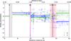 |
Fig. 9 LOS decomposition of starlight polarization by TRIShUL toward Galactic open cluster Berkeley 19 in the (q, u) − μ plane. The color scheme follows that of Fig. 8. The black point denotes the mean parallax of the cloud as inferred from the posterior distribution of BISP-1, with the error bar representing the standard deviation. |
6 Summary and conclusion
In this work, we introduced and demonstrated TRIShUL, a novel, data-driven method for tomographic decomposition of the magnetized ISM using starlight polarization. Developed using a frequentist framework, the method is both conceptually straightforward and computationally efficient. TRIShUL employs a unique combination of cumulative Mahalanobis distance as a function of distance-sorted indices to detect structural breaks that indicate the presence of dust layers along the LOS. This cumulative approach allows for reliable detections of dust layers, even those inducing weak polarization and in low S/N conditions. The effectiveness of the cumulative approach has also been recently demonstrated by Zhang et al. (2025) in identifying extinction jumps along the LOS for constructing 3D extinction maps. However, their strategy is not directly applicable to polarization. Unlike extinction, which increases monotonically and whose cumulative differences from the mean can enhance discontinuities, polarization can exhibit depolarization effects, making the averaging approach unreliable. Tests with our simulated data confirm that the same algorithm is unable to identify the correct break in polarization.
While the cumulative process enhances sensitivity to subtle structural changes, it may also introduce spurious breaks caused by local fluctuations in Mahalanobis distance, attributable to measurement uncertainties or scatter in the data. To address this, we designed a robust strategy to eliminate such false detections. We estimated average parallaxes and Stokes parameters of the identified layers, incorporating a full error budget to quantify both statistical and systematic uncertainties. This enabled reliable inference of physical properties such as cloud distance, degree of polarization, position angle, or the orientation of the POS magnetic field. The entire framework, including Maha-lanobis distance calculation, break detection (testing one to five breaks), spurious break rejection, and parameter estimation along the uncertainty intervals, completes in under two minutes on a laptop, highlighting its suitability for large-scale survey applications. One of the caveats of our method is that while we used uncertainties in the parallax in the rejection process, they were not considered in the identification of the breaks themselves.
We benchmarked and validated the performance of TRIShUL using synthetic polarization data constructed by Pelgrims et al. (2023). We showed that TRIShUL successfully recovers LOS dust clouds and their polarization properties as soon as the induced degree of polarization exceeds 0.1%. This correspond to having more than 10% of the stars lying in the background of the cloud or in between two clouds of LOS having 350 stars. It is important to note that our algorithm is able to detect structural breaks in the distance-sorted Mahalanobis distance even in extreme cases (low polarization (<0.1%) and low number statistics in the background of the cloud). However, such detections are typically excluded in the spurious layer rejection step because of their low statistical significance. This limits the sensitivity of the method to identify extremely weak features. Enhancements to address this regime will be explored in future work. Nevertheless, the current sensitivity limits of TRIShUL are well matched to the typical detection limits (∼0.1%) of most of the existing polarization instruments (e.g., Maharana et al. 2024).
We further demonstrated the applicability of TRIShUL to real observational data across diverse ISM environments - in a high Galactic latitude region and a region near the Galactic plane. In both cases, the estimated cloud distances and polarization properties are consistent with values reported in the literature, within uncertainties.
We conducted a detailed comparison between our method, TRIShUL, and the recently developed Bayesian inference-based algorithm, BISP-1, which performs fully automated tomographic decomposition of starlight polarization. We observed that BISP-1 generally yields more precise estimates due to its probabilistic framework, but they are sensitive to the choice of the priors on cloud parallaxes. In contrast, TRIShUL does not require any external prior information and provides results that are statistically robust, albeit with somewhat larger uncertainties.
Another key distinction between the two methods lies in their computational efficiency. TRIShUL employs a direct, data-driven frequentist approach to identify structural breaks and reject spurious ones. These processes are more intuitive and significantly faster for testing 1− to N− breaks, compared to BISP-1. BISP-1 requires extensive posterior sampling over a high-dimensional parameter space, and its computation time increases substantially as the number of model layers grows. However, unlike TRIShUL, BISP-1 has the advantage of both accounting for and modeling out the intrinsic scatter arising due to turbulence in the ISM, which is not currently estimated in our approach.
Overall, TRIShUL presents a computationally efficient, statistically robust, and prior-free multilayer decomposition approach for polarization tomography, well-suited for the upcoming era of large-scale polarization surveys. The complementary strengths of TRIShUL and BISP-1 can be effectively harnessed by combining the two methods. Initial results from TRIShUL can be used to inform the priors for BISP-1. This hybrid strategy enables fast, reliable decomposition with TRIShUL, followed by high-precision, statistically rigorous refinement through Bayesian inference.
Data availability
The code associated with this article is available on GithHub at the following link: https://github.com/NamitaU/TRIShUL
Acknowledgements
We thank the anonymous referees for the constructive comments. This research is funded by the European Union. Views and opinions expressed are, however, those of the author(s) only and do not necessarily reflect those of the European Union or the European Research Council Executive Agency. Neither the European Union nor the granting authority can be held responsible for them. This work is supported by an ERC grant, MW-ATLAS project no. 101166905. We thank Dr. G. V. Panopoulou for their constructive feedback. N.U. acknowledges support from the European Research Council (ERC) under the Horizon ERC Grants 2021 programme under grant agreement No. 101040021. K.T. acknowledges the support by the TITAN ERA Chair project (contract no. 101086741) within the Horizon Europe Framework Program of the European Commission. V.P. acknowledges funding from a Marie Curie Action of the European Union (grant agreement No. 101107047). N.U. would like to thank D. Blinov for discussions and insights from the coding perspective.
References
- Akaike, H. 1974, IEEE Trans. Automat. Control, 19, 716 [Google Scholar]
- Andersson, B. G., & Potter, S. B. 2005, MNRAS, 356, 1088 [Google Scholar]
- Andersson, B. G., Lazarian, A., & Vaillancourt, J. E. 2015, ARA&A, 53, 501 [Google Scholar]
- Angarita, Y., Versteeg, M. J. F., Haverkorn, M., et al. 2025, AJ, 170, 57 [Google Scholar]
- Bai, J., & Perron, P. 2002, J. Appl. Econometrics, 18, 1 [Google Scholar]
- Bailer-Jones, C. A. L., Rybizki, J., Fouesneau, M., Demleitner, M., & Andrae, R. 2021, AJ, 161, 147 [Google Scholar]
- Bailey, J., Lewis, F., Howarth, I. D., et al. 2024, ApJ, 972, 103 [NASA ADS] [CrossRef] [Google Scholar]
- Beck, R. 2015, A&A Rev., 24, 4 [Google Scholar]
- Beck, R., & Wielebinski, R. 2013, in Planets, Stars and Stellar Systems, Galactic Structure and Stellar Populations, eds. T. D. Oswalt, & G. Gilmore (Berlin: Springer), 5, 641 [Google Scholar]
- Bijas, N., Eswaraiah, C., Sandhyarani, P., Jose, J., & Gopinathan, M. 2024, MNRAS, 529, 4234 [CrossRef] [Google Scholar]
- Chiang, Y.-K. 2023, ApJ, 958, 118 [NASA ADS] [CrossRef] [Google Scholar]
- Clark, S. E., & Hensley, B. S. 2019, ApJ, 887, 136 [NASA ADS] [CrossRef] [Google Scholar]
- Clarke, D. 2010, Stellar Polarimetry (Boschstrasse: Wiley-VCH Verlag) [Google Scholar]
- Clemens, D. P., Pinnick, A. F., Pavel, M. D., & Taylor, B. W. 2012, ApJS, 200, 19 [Google Scholar]
- Cotton, D. V., Bailey, J., Kedziora-Chudczer, L., et al. 2016, MNRAS, 455, 1607 [NASA ADS] [CrossRef] [Google Scholar]
- Dickey, J. M., West, J., Thomson, A. J. M., et al. 2022, ApJ, 940, 75 [NASA ADS] [CrossRef] [Google Scholar]
- Doi, Y., Hasegawa, T., Bastien, P., et al. 2021, ApJ, 914, 122 [NASA ADS] [CrossRef] [Google Scholar]
- Doi, Y., Nakamura, K., Kawabata, K. S., et al. 2024, ApJ, 961, 13 [NASA ADS] [CrossRef] [Google Scholar]
- Edenhofer, G., Zucker, C., Frank, P., et al. 2024, A&A, 685, A82 [NASA ADS] [CrossRef] [EDP Sciences] [Google Scholar]
- Fridman, P. A. 2010, MNRAS, 409, 808 [NASA ADS] [CrossRef] [Google Scholar]
- Gaia Collaboration (Brown, A. G. A., et al.) 2018, A&A, 616, A1 [NASA ADS] [CrossRef] [EDP Sciences] [Google Scholar]
- Gaia Collaboration (Vallenari, A., et al.) 2023, A&A, 674, A1 [NASA ADS] [CrossRef] [EDP Sciences] [Google Scholar]
- Green, G. M., Schlafly, E., Zucker, C., Speagle, J. S., & Finkbeiner, D. 2019, ApJ, 887, 93 [NASA ADS] [CrossRef] [Google Scholar]
- Hall, J. S. 1949, Science, 109, 166 [NASA ADS] [CrossRef] [Google Scholar]
- Hensley, B. S., & Draine, B. T. 2021, ApJ, 906, 73 [NASA ADS] [CrossRef] [Google Scholar]
- Hiltner, W. A. 1949, Science, 109, 165 [NASA ADS] [CrossRef] [Google Scholar]
- Hotelling, H. 1992, The Generalization of Student’s Ratio (New York: Springer), 54 [Google Scholar]
- Jaffe, T. R. 2019, Galaxies, 7, 52 [NASA ADS] [CrossRef] [Google Scholar]
- Jansson, R., & Farrar, G. R. 2012, ApJ, 757, 14 [NASA ADS] [CrossRef] [Google Scholar]
- Korochkin, A., Semikoz, D., & Tinyakov, P. 2025, A&A, 693, A284 [NASA ADS] [CrossRef] [EDP Sciences] [Google Scholar]
- Lallement, R., Babusiaux, C., Vergely, J. L., et al. 2019, A&A, 625, A135 [NASA ADS] [CrossRef] [EDP Sciences] [Google Scholar]
- Lallement, R., Vergely, J. L., Babusiaux, C., & Cox, N. L. J. 2022, A&A, 661, A147 [NASA ADS] [CrossRef] [EDP Sciences] [Google Scholar]
- Lenz, D., Hensley, B. S., & Doré, O. 2017, ApJ, 846, 38 [NASA ADS] [CrossRef] [Google Scholar]
- Lombard, F., & Koen, C. 1993, MNRAS, 263, 309 [Google Scholar]
- Magalhães, A. M., Pereyra, A., Melgarejo, R., et al. 2005, ASP Conf. Ser., 343, 305 [Google Scholar]
- Maharana, S., Blinov, D., Ramaprakash, A. N., Pavlidou, V., & Tassis, K. 2024, SPIE Conf. Ser., 13096, 130963A [Google Scholar]
- Panopoulou, G. V., Tassis, K., Skalidis, R., et al. 2019, ApJ, 872, 56 [NASA ADS] [CrossRef] [Google Scholar]
- Panopoulou, G. V., Markopoulioti, L., Bouzelou, F., et al. 2025, ApJS, 276, 15 [NASA ADS] [CrossRef] [Google Scholar]
- Patat, F., Maund, J. R., Benetti, S., et al. 2010, A&A, 510, A108 [NASA ADS] [CrossRef] [EDP Sciences] [Google Scholar]
- Pattle, K., Fissel, L., Tahani, M., Liu, T., & Ntormousi, E. 2023, ASP Conf. Ser., 534, 193 [NASA ADS] [Google Scholar]
- Pavel, M. D. 2014, AJ, 148, 49 [NASA ADS] [CrossRef] [Google Scholar]
- Pelgrims, V., Ferrière, K., Boulanger, F., Lallement, R., & Montier, L. 2020, A&A, 636, A17 [EDP Sciences] [Google Scholar]
- Pelgrims, V., Panopoulou, G. V., Tassis, K., et al. 2023, A&A, 670, A164 [NASA ADS] [CrossRef] [EDP Sciences] [Google Scholar]
- Pelgrims, V., Mandarakas, N., Skalidis, R., et al. 2024, A&A, 684, A162 [NASA ADS] [CrossRef] [EDP Sciences] [Google Scholar]
- Pelgrims, V., Unger, M., & Mar⅛, I. C. 2025, A&A, 695, A148 [NASA ADS] [CrossRef] [EDP Sciences] [Google Scholar]
- Planck Collaboration Int. XLVIII. 2016, A&A, 596, A109 [NASA ADS] [CrossRef] [EDP Sciences] [Google Scholar]
- Rezaei Kh., S., Bailer-Jones, C. A. L., Soler, J. D., & Zari, E. 2020, A&A, 643, A151 [EDP Sciences] [Google Scholar]
- Schlegel, D. J., Finkbeiner, D. P., & Davis, M. 1998, ApJ, 500, 525 [Google Scholar]
- Schwarz, G. 1978, Annals Stat., 6, 461 [Google Scholar]
- Skalidis, R., & Pelgrims, V. 2019, A&A, 631, L11 [NASA ADS] [CrossRef] [EDP Sciences] [Google Scholar]
- Speagle, J. S. 2020, MNRAS, 493, 3132 [Google Scholar]
- Sun, X. H., Reich, W., Waelkens, A., & Enßlin, T. A. 2008, A&A, 477, 573 [NASA ADS] [CrossRef] [EDP Sciences] [Google Scholar]
- Tahani, M., Plume, R., Brown, J. C., & Kainulainen, J. 2018, A&A, 614, A100 [NASA ADS] [CrossRef] [EDP Sciences] [Google Scholar]
- Tahani, M., Glover, J., Lupypciw, W., et al. 2022, A&A, 660, L7 [NASA ADS] [CrossRef] [EDP Sciences] [Google Scholar]
- Tassis, K., Ramaprakash, A. N., Readhead, A. C. S., et al. 2018, arXiv e-prints [arXiv:1810.05652] [Google Scholar]
- Tritsis, A., & Tassis, K. 2018, Science, 360, 635 [Google Scholar]
- Unger, M., & Farrar, G. R. 2024, ApJ, 970, 95 [NASA ADS] [CrossRef] [Google Scholar]
- Uppal, N., Ganesh, S., Pelgrims, V., Joshi, S., & Sarkar, M. 2024, A&A, 690, A49 [NASA ADS] [CrossRef] [EDP Sciences] [Google Scholar]
- Vallat, R. 2018, J. Open Source Softw., 3, 1026 [NASA ADS] [CrossRef] [Google Scholar]
- Vergely, J. L., Lallement, R., & Cox, N. L. J. 2022, A&A, 664, A174 [NASA ADS] [CrossRef] [EDP Sciences] [Google Scholar]
- Versteeg, M. J. F., Magalhães, A. M., Haverkorn, M., et al. 2023, AJ, 165, 87 [NASA ADS] [CrossRef] [Google Scholar]
- Ward, K., Dilillo, G., Eckley, I., & Fearnhead, P. 2022, arXiv e-prints [arXiv:2208.01494] [Google Scholar]
- Wolleben, M., Fletcher, A., Landecker, T. L., et al. 2010, ApJ, 724, L48 [NASA ADS] [CrossRef] [Google Scholar]
- Zeileis, A., Leisch, F., Hornik, K., & Kleiber, C. 2002, J. Stat. Softw., 7, 1 [CrossRef] [Google Scholar]
- Zeileis, A., Kleiber, C., Krämer, W., & Hornik, K. 2003, Comput. Stat. Data Anal., 44, 109 [CrossRef] [Google Scholar]
- Zhang, S., Su, Y., Chen, X., et al. 2025, AJ, 170, 185 [Google Scholar]
The choice of cloud parallax priors must be made with caution. We tested comparing models with different prior settings for the layers in each model, independently of each other. This resulted in 56 out of 60 cases incorrectly favoring a single-layer model (FNs), despite the presence of two layers.
Appendix A Nature of flagged cases
As described in Sect. 2.3, we flag sight lines as flag of "1," where a break passes the statistical significance test (i.e., the null hypothesis is rejected) in only one direction, either forward or backward, but not both. This situation typically arises when the breakpoint-detection algorithm, prior to any rejection step, misses the true cloud location and instead identifies a nearby spurious break caused by local fluctuations in the cumulative Mahalanobis distance. Since the segmentation boundaries are updated dynamically, rejecting a break early in the sequence reshapes subsequent segment boundaries and can affect the outcome of the test for later breaks. Hence, a break that appears significant in one direction might not be confirmed when tested from the opposite direction.
In most single-cloud mock samples, a common type of flagged case is observed when a break identified in the forward pass is rejected in the backward (or vice versa) while a different break is selected in the reverse direction by rejecting null-hypothesis at the same confidence level. In such cases, the algorithm outputs two different breaks, both of which are flagged as "1." Although the identified breakpoints differ, they consistently indicate the presence of only one cloud layer in both analysis direction. Therefore, such cases should not be considered as FPs. Rather, they reflect an underlying detection, where the presence of one layer is real but its precise location is uncertain due to inaccuracies in the initial identification of the breaks by the strucchange breakpoint algorithm. An example of this behavior is shown in Fig. A.1, where the mock sample contains a single cloud at approximately 790 pc, inducing a polarization of 0.1%. In this case, 50% of the stars lie behind the cloud.
We applied TRIShUL on this dataset, and the struccha-nge breakpoint-detection algorithm identifies five breaks in the distance-sorted cumulative Mahalanobis distance profile, marked by vertical blue lines in the top panel. However, none of these breaks align with the true cloud location, possibly due to the dominance of fluctuation in the cumulative profile over the actual polarization signal. The rejection step eliminates all but the fourth break in the forward pass, while in the backward pass, the fourth break is rejected in favor of the third one. As a result, the algorithm outputs both the third and fourth breaks, but flags them as uncertain. The final solution, displayed in the qu-μ plane, is shown in the bottom panel of Fig. A.1. In cases involving two or more clouds, the number of flagged cases is expected to increase, as similar ambiguity can be shown by one or more breaks along the LOS.
In many such cases, one of the identified breaks can be discarded by examining the estimated polarization to see if it is consistent with zero within the uncertainties, and by recomputing the cloud parameters based only on the remaining break. A more recommended approach is to rerun TRIShUL with modified-breakpoint detection parameters, such as increasing the maximum number of allowed breaks to better capture the true transition or adjusting the minimum number of stars per segment. For the illustrated example, increasing the maximum number of breakpoints to ten successfully resolves the flagged case.
Appendix B Effect of inclination angle of magnetic field on the performance of our method
In this section, we examine the effect of the inclination angle of the magnetic field with POS on the performance of our method. Similar simulated data are generated as described in Sect. 3.1 but with inclination angle γBreg sampled from 0° to 75° in 15° steps, and pmax adjusted to keep the observed polarization pc ≈ 0.2%. For each configuration, 10 realizations are generated by varying the POS orientation of the magnetic field ψBreg, resulting in a total of 300 samples.
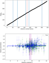 |
Fig. A.1 Example of a flagged reconstruction case. Top panel: Breakpoints (vertical blue lines) identified by the strucchange package in the distance-sorted cumulative Mahalanobis distance profile. Bottom panel: LOS decomposition in the qu-μ plane (q in green, while u in blue). The dashed red line in the top panel and the dashed gray line in the bottom panel indicate the true location of the input dust layer. |
We performed LOS tomography decomposition of starlight polarization using our method, testing a maximum of five breaks and a minimum of five stars per segment. Among the 300 tested samples, approximately 15% resulted in FNs. As shown in the top-most panel of Fig. B.1, these failures are predominantly associated with cases where f bg = 10%, similar to the results shown in Sect. 3.1. Only 3% of the cases led to FPs, illustrated in the second panel. About 8.6% of the cases are flagged as uncertain and require further analysis, while the remaining 74% successfully identified a single cloud with high statistical confidence (see the bottom panel of Fig. B.1).
To assess the influence of magnetic field inclination on the accuracy of estimated parameters from our method, we computed the deviations of the estimated values (parallax and Stokes parameters) from corresponding true values, following Sect. 3.1 and plotted in Fig B.2. The results are consistent with those shown in Fig. 4 for single-cloud scenarios. No clear dependency of estimated parameters on the inclination angle for a fixed fbg is observed in the figure. The dominant factor affecting the accuracy of the estimated parameters remains the background star fraction (f bg), i.e., the method often fails to detect the layer when only 10% of stars are located behind the cloud. The figure shows increased scatter and larger uncertainties in the estimated cloud parallax for fbg = 90% and the same effect in polarization properties (q and u), but for fbg = 10%; these trends are discussed in detail in Sect. 3.1.
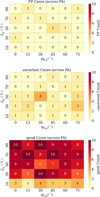 |
Fig. B.1 Distribution of decomposition outcomes (FP, FN, flagged, and reliable) for 300 single-cloud mock sight lines, plotted as a function of inclination angle of magnetic field (γBref) and background star fraction (fbg) across ten different position angle of the POS magnetic field. |
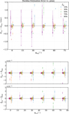 |
Fig. B.2 Difference in the estimated parameters, parallax (top panel) and Stokes parameter (bottom panel), of the identified clouds with corresponding true values as a function of inclination angle of magnetic field (γBreg). The dashed black line is the reference for a perfect match between estimated and true values. |
Appendix C Classification statistics for single-cloud mock samples
The distribution of the number of FN, FP, flagged, and reliable cases based on the number of clouds recovered in the LOS tomography of starlight polarization in 450 single cloud mock samples is presented in Fig. C.1. The results are presented as a function of the input polarization signal (pinput), i.e., the maximum polarization induced by the cloud on background stars, and the fraction of stars located behind the cloud (f bg). A detailed discussion and interpretation of these results is provided in Sect. 3.1.
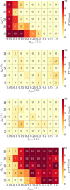 |
Fig. C.1 Distribution of decomposition outcomes (FN, FP, flagged, and reliable) for 450 single-cloud mock sight lines plotted as a function of input polarization strength (pinput) and background star fraction (fbg). |
Appendix D Classification statistics for two-cloud mock samples
For the two cloud scenario, we generate 1200 sample, each corresponds to a unique combination of three input parameters: the maximum polarization induced by the second (farther) cloud ( ), the relative position angle of magnetic field in second cloud with respect to the nearby (∆ψ), and the fraction of stars that are background of nearby cloud that are also background of second cloud, (fbg2). For each parameter combination, five random realizations were generated. The number of cases with FNs resulting from the LOS tomography decomposition of starlight polarization for using TRIShUL are shown in Fig. D.1. To visualize the joint impact of these variables, the results are displayed in panels grouped by fbg2, with
  on the X-axis and ∆ψ on the Y -axis. The implications and interpretation of these results are addressed in Sect. 3.2
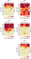 |
Fig. D.1 Distribution of FN decomposition results for 1200 two-cloud mock samples using TRIShUL. The statistics represents the resulted FN for five random samples of input combination of background star fraction (fbg2, separate panels), maximum polarization of second cloud ( |

All Tables
Comparison of polarization properties of clouds estimated from our method with results from the literature.
All Figures
|
Fig. 1 Top left: q (in green) and u (in blue) as a function of distance-sorted stellar indices in a simulated LOS, without incorporating turbulence (internal scattering) and measurement uncertainties. Middle and bottom left: corresponding Mahalanobis distance (dMaha) and its cumulative effect ( |
| In the text | |
|
Fig. 2 Breakpoints (blue lines) detected in the distance-sorted cumulative Mahalanobis distance profiles using the R strucchange package. Top panel: results for mock data shown in the bottom-left panel of Fig. 1. Bottom panel: results for the mock data shown in the bottom-right panel of Fig. 1. The vertical dashed red lines indicate the input distances of the dust layers used in the simulations. |
| In the text | |
|
Fig. 3 Heat map illustrating the number of FNs out of 450 single-cloud mock samples, each with a combination of pinput and fbg, evaluated across ten samples of ψ ranging from 0° to 180°. The color intensity and the number within each cell represent the resulting count of FNs. |
| In the text | |
|
Fig. 4 Performance of TRIShUL as a function of input polarization signal for different cloud distances probed by fbg (in different colors). Top panel: difference between the estimated parallax (ϖest) and the parallax of the star closest to the input layer (ϖtrue). Bottom panel: difference in estimated Stokes parameters (qest, uest) from the corresponding true values (qtrue, utrue). The results corresponding to different fbg are shifted by 0.02% on the X-axis for visual clarity. Horizontal dashed lines are the references to a perfect match between estimated and true parameters. |
| In the text | |
|
Fig. 5 Performance testing of our method in recovering parallax (top panel) and Stokes parameters (bottom panel) of both layers in two-cloud sample tests. The color scheme is defined for different sets of fbg2 and is similar to fbg in Fig. 4. The horizontal dashed lines correspond to a perfect match between the estimated and true values. The open black circles indicate cases where an additional, spurious layer beyond the second layer is identified, while the first layer is missed. Additional details about the figure are provided in the text in Sect. 3.2. |
| In the text | |
|
Fig. 6 Comparison of estimated parameters from BISP-1 (black) and TRIShUL (red) with the true values (blue) for parallax (top panel) and Stokes parameters (bottom panel) in one-cloud mock catalogs. |
| In the text | |
|
Fig. 7 Comparison of the estimated parameters from BISP-1 (black points) and TRIShUL (red points) with the true value (blue points) for parallax (top panel) and the Stokes parameters (bottom panel) of mock catalogs with two clouds. The open dark-blue circles indicate the flagged cases in TRIShUL and open black squares correspond to FNs in BISP-1. |
| In the text | |
|
Fig. 8 LOS decomposition of starlight polarization by TRIShUL displayed in (q, u) − μ (q in green, u in blue) plane for the polarization data from Panopoulou et al. (2019). The vertical lines indicate the positions of the cloud layers estimated by our method, with the shaded regions representing statistical (pink) and systematic (gray) uncertainties. Top panel: one-cloud region. Bottom panel: two-cloud region. The estimated distance range from Panopoulou et al. (2019) and Pelgrims et al. (2023) are marked in orange and black as GP19 and VP23, respectively. |
| In the text | |
|
Fig. 9 LOS decomposition of starlight polarization by TRIShUL toward Galactic open cluster Berkeley 19 in the (q, u) − μ plane. The color scheme follows that of Fig. 8. The black point denotes the mean parallax of the cloud as inferred from the posterior distribution of BISP-1, with the error bar representing the standard deviation. |
| In the text | |
|
Fig. A.1 Example of a flagged reconstruction case. Top panel: Breakpoints (vertical blue lines) identified by the strucchange package in the distance-sorted cumulative Mahalanobis distance profile. Bottom panel: LOS decomposition in the qu-μ plane (q in green, while u in blue). The dashed red line in the top panel and the dashed gray line in the bottom panel indicate the true location of the input dust layer. |
| In the text | |
|
Fig. B.1 Distribution of decomposition outcomes (FP, FN, flagged, and reliable) for 300 single-cloud mock sight lines, plotted as a function of inclination angle of magnetic field (γBref) and background star fraction (fbg) across ten different position angle of the POS magnetic field. |
| In the text | |
|
Fig. B.2 Difference in the estimated parameters, parallax (top panel) and Stokes parameter (bottom panel), of the identified clouds with corresponding true values as a function of inclination angle of magnetic field (γBreg). The dashed black line is the reference for a perfect match between estimated and true values. |
| In the text | |
|
Fig. C.1 Distribution of decomposition outcomes (FN, FP, flagged, and reliable) for 450 single-cloud mock sight lines plotted as a function of input polarization strength (pinput) and background star fraction (fbg). |
| In the text | |
|
Fig. D.1 Distribution of FN decomposition results for 1200 two-cloud mock samples using TRIShUL. The statistics represents the resulted FN for five random samples of input combination of background star fraction (fbg2, separate panels), maximum polarization of second cloud ( |
| In the text | |
Current usage metrics show cumulative count of Article Views (full-text article views including HTML views, PDF and ePub downloads, according to the available data) and Abstracts Views on Vision4Press platform.
Data correspond to usage on the plateform after 2015. The current usage metrics is available 48-96 hours after online publication and is updated daily on week days.
Initial download of the metrics may take a while.