| Issue |
A&A
Volume 705, January 2026
|
|
|---|---|---|
| Article Number | A109 | |
| Number of page(s) | 9 | |
| Section | Planets, planetary systems, and small bodies | |
| DOI | https://doi.org/10.1051/0004-6361/202556779 | |
| Published online | 12 January 2026 | |
Probing methane in Uranus’ upper stratosphere using HST observations of the 1280 Å Raman feature
1
Royal Institute of Technology (KTH),
Stockholm,
Sweden
2
LATMOS-IPSL, UVSQ Paris Saclay, Sorbonne Université, CNRS,
France
3
Southwest Research Institute,
San Antonio,
TX,
USA
4
Department of Earth and Planetary Sciences, The Johns Hopkins University,
Baltimore,
MD,
USA
5
LIRA, Observatoire de Paris, Université PSL, Sorbonne Université, Université Paris Cité, Cergy Paris Université, CNRS,
Meudon,
France
6
Aix Marseille Université, CNRS, CNES, LAM,
Marseille,
France
★ Corresponding author: This email address is being protected from spambots. You need JavaScript enabled to view it.
Received:
7
August
2025
Accepted:
31
October
2025
Abstract
We analysed far-ultraviolet (FUV) spectra of Uranus obtained by the HST STIS and COS instruments in 2012 and 2014, respectively, to determine the brightness of Raman-scattered Lyman-alpha (Lyα) emissions centred at 1280 Å (hereafter, the Raman feature). The Raman feature is unique among the Solar System’s giant planets and forms in Uranus’ atmosphere due to weak vertical mixing of hydrocarbons with H2, leading to efficient Rayleigh–Raman scattering. Methane is the dominant hydrocarbon species on Uranus, and since it absorbs FUV radiation, it affects the Rayleigh–Raman scattering of Lyα photons by H2 and, eventually, the brightness of the Raman feature. We derive a brightness of 20−6+1 R from the STIS data, which is similar to the brightness measured by Voyager 2 UVS during the 1986 flyby of Uranus, when considering the suggested recalibration of UVS measurements by a factor of ∼0.5. Based on the observed brightness, we constrain the upper altitude (pressure) level for the abundance of methane in the upper atmosphere using radiative transfer simulations that include resonant scattering by H, Rayleigh–Raman scattering by H2, and absorption by CH4. We considered the solar Lyα flux as the source of Lyα radiation at Uranus. We find that resonant scattering by H significantly affects Rayleigh–Raman scattering by H2 and thus the modelled brightness of the Raman feature. We derive methane profiles by obtaining the simultaneous fit to the observed Lyα, as well as the 1280 Å brightness of Uranus. Methane appears to be depleted (number density becomes less than 1 cm−3) above the altitude (pressure) range of ∼478–515 km (4 × 10⁻³–2.4 × 10⁻³ mbar), while the Lyα absorption optical depth reaches unity for methane in the altitude (pressure) range of ∼237–257 km (2.54 × 10⁻¹–1.65 × 10⁻¹ mbar). When neglecting resonant scattering by H, the methane depletion must be deeper in the atmosphere at an altitude (pressure) of ∼395 km (1.4 × 10⁻² mbar), similar to previous findings based on Voyager 2 observations of the feature. The analysis of the Raman feature provides independent CH4 constraints in the upper atmosphere for detailed photochemistry modelling and highlights the importance of UV instruments for the future Uranus Orbiter and Probe (UOP) mission.
Key words: radiative transfer / methods: numerical / techniques: spectroscopic / planets and satellites: atmospheres / planets and satellites: gaseous planets
© The Authors 2026
 Open Access article, published by EDP Sciences, under the terms of the Creative Commons Attribution License (https://creativecommons.org/licenses/by/4.0), which permits unrestricted use, distribution, and reproduction in any medium, provided the original work is properly cited.
This article is published in open access under the Subscribe to Open model. This email address is being protected from spambots. You need JavaScript enabled to view it. to support open access publication.
1 Introduction
In a planetary atmosphere dominated by molecular hydrogen (H2), efficient Rayleigh–Raman scattering of Lyman-alpha (Lyα, 1215.67 Å) photons can occur. The Lyα line is one of the brightest solar lines in the far-ultraviolet (FUV) wavelength range. Therefore, observations of planetary Rayleigh–Raman emissions driven by the incident Lyα flux can serve as an excellent tool for understanding planetary atmospheres. During the scattering of a Lyα photon by H2, there is a ∼0.86 probability that the photon is Rayleigh scattered, thus retaining the same wavelength (at temperature T = 300 K, Ford & Browne 1973). Accordingly, there is ∼0.14 probability that a part of the incoming Lyα photon’s energy excites ro-vibrational states of the molecule, leading to scattered photons with energies different from the Lyα photon. These are the Raman-scattered Lyα emissions by H2. Among these, the Raman-scattered emission centred at 1280 Å (involving the transition H2(v = 0) → H2(v = 1)) is the brightest, with ∼0.086 probability that Lyα photons scatter to this emission.
As the atmospheres of the Solar System’s giant planets are dominated by H2, studies such as Brandt (1963) and Jenkins (1969) suggested the possibility of observing Rayleigh–Raman-scattered Lyα emissions in these atmospheres. However, soon after, Carlson & Judge (1971) showed that at Jupiter these emissions would be very weak and thus almost unobservable. This was later confirmed by Voyager 2 extreme ultraviolet observations of Jupiter (Sandel et al. 1979), and similarly for Saturn (Sandel et al. 1982) and Neptune (Broadfoot et al. 1989). Apart from hydrogen and helium, giant planet atmospheres also contain significant amounts of hydrocarbons, which are efficient absorbers of ultraviolet photons. Voyager 2 observations showed that in the atmospheres of Jupiter, Saturn, and Neptune, hydrocarbons exist in high abundance at altitudes where significant Rayleigh scattering by H2 can occur, and thus they absorb most of the Rayleigh–Raman-scattered ultraviolet photons by H2. Thus, contrary to the prediction of Brandt (1963), no significant Rayleigh and Raman scattering was observed in these atmospheres.
The first ultraviolet observations of Uranus were obtained using the International Ultraviolet Explorer (IUE) observatory. From observations taken between March 1982 and September 1985, Clarke et al. (1986) reported an average Lyα brightness of 1400 ± 450 R. They estimated that 200 R was contributed by resonant scattering by H and Rayleigh scattering by H2. However, they could not identify Raman emissions in the IUE spectra and placed an upper limit of 30 R on the Raman emissions centred at 1280 Å. The Voyager 2 spacecraft flew by Uranus in 1986, during the planet’s southern solstice, as shown in Fig. 1. During this flyby, the first close-in FUV observations were obtained using the Ultraviolet Spectrometer (UVS) instrument, and Broadfoot et al. (1986) indeed detected the 1280 Å feature (hereafter, the Raman feature) in UVS observations of Uranus. Yelle et al. (1987) explained this feature as the Raman-scattered Lyα by H2, involving the H2(v = 0) → H2(v = 1) transition, and determined the brightness to be 40 ± 20 R. This feature is unique among the giant planets of the Solar System. It indicates efficient Rayleigh–Raman scattering of UV radiation in Uranus’ atmosphere, and Yelle et al. (1987) estimated that the Uranian atmosphere is devoid of absorbing hydrocarbons at pressures less than 0.5 mbar. Unlike other giant planets, at Uranus, due to the weak vertical mixing of hydrocarbons with H2 (resulting from a lower eddy diffusion coefficient, Kzz) and the extended atmosphere, efficient FUV Rayleigh–Raman scattering by H2 is possible (Herbert et al. 1987; Yelle et al. 1989; Strobel et al. 1991; Herbert & Sandel 1999). The cause of lower eddy diffusion in the Uranian atmosphere might be the planet’s weak internal heating (Pearl et al. 1990). How this lower eddy diffusion affects the hydrocarbon transport at Uranus is an area of active research.
Methane (CH4) is the most abundant hydrocarbon in Uranus’ atmosphere. Using Voyager 2 radio occultation measurements, Lindal et al. (1987) derived the methane profile from 0.66 to 2.3 bars, with methane mole fraction increasing from 0.04% at 0.66 bars to a constant value of 2.26% below 1.3 bar (see their Table 1). Using the observations of Uranus obtained from the Hubble Space Telescope’s (HST) Space Telescope Imaging Spectrograph (STIS) instrument in 2002, Karkoschka & Tomasko (2009) estimated the methane mole fraction value in the deeper atmosphere to be ∼3.2%. Although the methane abundance in the deeper atmosphere is significant (several percent), methane condenses at the tropopause (∼100 mbar) due to low atmospheric temperatures. The small amount of methane transported upwards into the stratosphere undergoes photolysis by ultraviolet photons, leading to photochemical production of heavier hydrocarbons such as acetylene (C2H2), ethylene (C2H4), ethane (C2H6), propyne or methylacetylene (CH3C2H), and diacetylene (C4H2) (see, e.g. Atreya & Ponthieu 1983; Bishop et al. 1990; Burgdorf et al. 2006).
To explain the measured 1280 Å Raman emission, Yelle et al. (1987) explored methane profiles based on an isothermal transport model. They derived that a methane profile with a constant upward flux of 3 × 108 cm−2s−1 and Kzz of 200 cm2s−1 between 1 mbar and 100 mbar agreed with the measured Raman brightness. Several subsequent studies revised the hydrocarbon abundances and Kzz values, finding that Kzz in Uranus’ atmosphere is higher than that deduced by Yelle et al. (1987). A review of these studies can be found in Orton et al. (2014). Using data from the Spitzer Infrared Spectrometer obtained during the 2007 equinox and a 1D photochemical model, Orton et al. (2014) derived the vertical profiles of the main hydrocarbons, such as CH4, C2H6, C2H2, CH3C2H, and C4H2 in the atmosphere of Uranus. They explored both constant and variable Kzz profiles to study vertical mixing in the atmosphere. Their model profile with a uniform Kzz of 2430 cm2s−1 and a tropopause CH4 mole fraction of 1.6 × 10⁻⁵, provided the best agreement with the observed CH4 and C2H6 emission spectra. Using this ‘nominal’ model, they constrained the CH4 abundance above 1.78 ± 0.2 bars, below which they set the ‘deep’ methane mole fraction to 3.2%.
Orton et al. (2014) deduced that different sloped-Kzz models for various tropopause CH4 mole fraction and Kzz combinations fit the Spitzer data equally well. Although their observations did not provide evidence of changes in hydrocarbon abundances from 1996 to 2007, their derived C2H2 abundance was much higher than that determined from the 1986 Voyager UVS solar occultation (Bishop et al. 1990). They suggested further research to determine whether this increase is due to genuine changes in atmospheric mixing or circulation, and whether seasonal variations in Kzz are required to influence the hydrocarbon column abundances, possibly in addition to photochemical changes. Shortly after, Lellouch et al. (2015) deduced a new average methane profile using observations of methane rotational lines from 2009–2011 obtained by the Herschel Space Telescope. To explain these observations, they required a methane profile with a tropopause-lower-stratosphere mole fraction of ∼9 × 10⁻⁴, which is substantially higher than that derived by Orton et al. (2014) from the Spitzer data. Lellouch et al. (2015) argue that this could be due to latitudinal inhomogeneities in the upper tropospheric and stratospheric methane abundances, with lower latitudes having higher abundance than higher latitudes. This latitudinal variation may result from upwelling at lower latitudes and downwelling at higher latitudes. Additionally, Herschel data probe more globally averaged conditions, whereas Spitzer data are more sensitive to warmer regions of the planet (Lellouch et al. 2015).
The newly derived temperature and methane profiles by Orton et al. (2014) and methane mixing ratios by Lellouch et al. (2015) prompted Sromovsky et al. (2019) to reanalyse HST/STIS observations of Uranus from 2002 and 2012. They revised their previously published values of methane volume mixing ratios in the deep atmosphere (Sromovsky et al. 2014), however, they maintained their inference about the relative variation in the upper tropospheric methane mixing ratio from low to high latitudes. They found that the mixing ratio decreases by a factor of three between 30◦ N and 70◦ N, accompanied by an increase in the effective depletion depth over this latitude range. This variation in the upper tropospheric methane mixing ratio was also observed in the latitudinally resolved observations of Uranus from 2001–2007 by the ground-based Hale Telescope and the Palomar High Angular Resolution Observer near-infrared adaptive optics camera system, as analysed by Roman et al. (2018). From mid-infrared observations obtained from the VLT in September and October 2018, Roman et al. (2020) infer an increase in the acetylene mole fraction at mid-latitudes by a factor of five compared to that deduced by Orton et al. (2014). They explain that this increase could result from efficient methane transport from the troposphere through the tropopause cold trap into the stratosphere at the mid-latitudes, owing to the tropospheric circulation pattern described by Flasar et al. (1987) based on Voyager 2 data.
Moses et al. (2018) studied the distribution of stratospheric hydrocarbons as a function of altitude, latitude, and season on Uranus using a time-variable 1D photochemical model. They find that photochemical mechanisms alone are not expected to produce significant seasonal variations in hydrocarbon abundances. However, they suggest that changes in vertical transport or in stratospheric circulation in general might lead to seasonal variations in hydrocarbon abundances. Thus, studies so far indicate that the hydrocarbon abundances in Uranus’ stratosphere and upper troposphere vary, and these variations are more likely due to seasonal changes in hydrocarbon vertical transport. This highlights the importance of assessing hydrocarbon abundances at different epochs in Uranus’ orbit.
Within HST observing campaign 13012, Uranus was observed using STIS and an FUV spectrum containing the 1280 Å feature was obtained. In programme 14036, Uranus was observed with the Cosmic Origins Spectrograph (COS), which also provided a spectrum that allows us to constrain emissions at 1280 Å. These observations were taken in 2012 and 2014, respectively, a few years after the 2007 equinox at Uranus. Figure 1 shows Uranus’ orientation as seen from Earth during the 2012 STIS observations. In addition to lower uncertainties, HST data also have a higher spectral resolution, sufficient to separate the bright and broad Lyα line from the 1280 Å Raman line. This was not the case for Voyager 2 observations, making it difficult to derive the Raman feature brightness. Additionally, recalibration of Voyager 2 UVS intensities (reduction by a factor of two; Quémerais et al. 2013) required a revision of the CH4 profiles derived from Voyager 2 data. In this study, we processed the STIS and COS FUV spectra of Uranus to derive the brightness of the 1280 Å feature and to estimate the altitude or pressure region above which the abundance of CH4 becomes negligible, using radiative transfer analysis for the Lyα and the 1280 Å Raman feature. Since CH4 is the main FUV absorber, with an abundance orders of magnitude larger than other hydrocarbons, and since our data do not allow us to individually determine the profiles of different hydrocarbon species, we focused on CH4 in our study. Joshi et al. (2025) recently published insights into Uranus’ upper atmosphere using Lyα images obtained by STIS in 1998 and 2011, reporting changes in brightness. The difference in off-disc brightness was attributed to changes in the H exosphere. The on-disc variation may be caused by changes in the abundances of H, H2 or CH4 or a combination thereof. The Raman feature in the FUV spectrum allowed us to constrain CH4 and thus contributes to understand possible seasonal variations in CH4 abundance.
In the following, we describe the observations and the derivation of the 1280 Å Raman feature brightness in Sect. 2. Our radiative transfer modelling is explained in Sect. 3. The results and discussion are presented in Sect. 4, and the summary and conclusions in Sect. 5.
 |
Fig. 1 Uranus as observed from Earth during the Voyager 2 flyby (left) and 2012 HST STIS observations (right). The orange lines indicate the STIS slit orientation with respect to Uranus’ disc. |
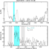 |
Fig. 2 Observations of Uranus with HST/STIS, using the G140L grating and 0.5″-wide slit separate emissions at the vibrational Raman branch around 1280 Å from other Uranus and geocorona emissions. The upper panel shows the spectral flux (averaged over the spatial y-axis) as a function of wavelength. The bottom panel shows the wavelength-integrated brightness in Rayleigh along the slit. The average emission on Uranus’ disc (light blue shading) is 25.5 R. An average background of 5.5 R was measured away from the disc in two regions (shaded grey) along the slit. |
2 Observations and data analysis
During the HST STIS campaign 13012, Uranus was observed with the G140L grating and the 0.5″-wide slit. This setup provides sufficient effective spectral resolution to separate the 1280 Å Raman feature from the bright oxygen geocorona emission at 1304 Å and the broad Lyα signal. Other emission features are discussed in more detail by Barthélemy et al. (2014). The first two exposures (data sets OBZ509010 and OBZ510010) in this mode, taken on September 28, 2012, suffered from high detector signal due to the dark current on the FUV-MAMA detector, which varies with time and temperature. A third exposure (OBZ512010) with this setup (G140L/0.5″) was taken on October 28, 2012 and exhibited a significantly lower detector signal. We read the data from the rectified spectral ‘x2d’ files, in which the spectral axis is perfectly aligned with the detector x-axis, and the long slit, with an effective length of 25″, is parallel to the detector y-axis. The orientation of the slit on the Uranian disc during this exposure is shown in Fig. 1.
The 2D detector image reveals bright geocorona emissions filling the entire slit at the H Lyα line and at the O triplet at 1304 Å. Emissions from Uranus’ upper atmosphere are furthermore detectable longward of ∼1530 Å (H2 band emissions) and at H Lyα. Apart from these emissions, the Raman-shifted emission at 1280 Å is the brightest in the spectrum and is clearly detectable. We used the trace of the H2 emissions to determine the planet’s position along the slit. Figure 2 shows the spectral flux from Uranus’ disc in R/Å (with 1 R = 106/4π photons/cm2/s/sr) between 1200 Å and 1550 Å, averaged over a region slightly larger than Uranus’ disc along the spatial y-axis.
We then extracted the emissions along the vertical (y) axis on the detector within the 0.5″-wide slit centred on 1280 Å and integrated them across the slit in the spectral direction to obtain the brightness in R as a function of the y slit position (see the lower panel in Fig. 2). Uranus’ disc had a diameter of 3.67″ on the observation day, covering 149 pixels around the centre pixel y=352 (light blue, Fig. 2 bottom). Towards larger y values, the detector background signal is more significant due to the dark currents on the FUV-MAMA detector mentioned above. To estimate the background level, we calculated the average background in areas on both sides of Uranus’ disc along the slit (shaded grey in Fig. 2). The average on-disc brightness is 25.5 R, with a propagated statistical error of 1.2 R. The background brightness is 5.5±0.3 R.
Subtracting this background, we obtain a residual brightness (with statistical uncertainty) from Uranus in the slit centred at 1280 Å of 20.0±1.3 R. In addition to the detector background, other emissions from Uranus may contribute to this signal, such as the continuum emission or the S(0) Raman branch at 1286 Å. The background-corrected Uranus brightness at wavelengths is approximately 4–6 R short of the 1280 Å slit region and 2–4 R towards longer wavelengths. Considering other potential emission contributions at this level (5 R), we derive a brightness of the 1280 Å Raman Q branch with statistical and systematic uncertainties of  , and use this value in the subsequent analysis.
The COS exposure obtained in campaign 14036 was taken on November 2, 2014 with the low-resolution grating G140L, which provides sufficient resolution (nominal 0.08 Å/pixel) for measuring the signal near 1280 Å. We detected a clear emission at 1280 Å, confirming the presence and persistence of the Raman feature at Uranus (Fig. 3). However, deriving a reliable brightness from the COS spectrum was hampered by the limitations of COS. The diameter of Uranus (∼3.7″) is larger than the nominal diameter of the round Primary Science Aperture (PSA) of 2.5″. Furthermore, the throughput function for the aperture is not a sharp step function at the edges; instead it decreases steadily from approximately 1″ from the centre pixel outwards. Without knowledge of the distribution of the brightness across Uranus and within the detector, it is difficult to convert the photons measured by COS into a disc-averaged brightness. Assuming unity aperture throughput over the aperture diameter, the detected flux suggests an areal brightness of ∼15 R, after subtracting a background determined from the fluxes shortward and longward of the 1280 Å feature (Fig. 3). We estimate a systematic uncertainty of 5 R from the assumptions about the spectral regions used for the Uranus and background signals, as well as from the uncertainties in the aperture throughput. This is consistent with the brightness derived from STIS above and, in particular, appears to confirm that the 1280 Å Raman Q branch emission brightness does not exceed ∼20 R. For further analysis, we adopted the Raman brightness value derived from the 2012 STIS data as the more reliable measurement with a well-defined error range.
Both the STIS and COS data sets also include Lyα emissions from Uranus extending to wavelengths below 1200 Å. However, it is difficult to extract reliable Lyα brightness of Uranus since the full disc is not captured in either data set and estimating the reference background emission is challenging. We therefore refrained from using the 2012 and 2014 data for a reference Lyα brightness and instead used the brightness measured in the STIS slitless images obtained in 2011 (Joshi et al. 2025).
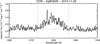 |
Fig. 3 Spectral region around 1280 Å in HST/COS exposure taken with the G140L grating on November 2, 2014. All flux within the vertical dotted lines was integrated to extract the 1280 Å brightness feature. The dashed line shows a linear fit to the adjacent spectral regions used to correct for background emissions. |
3 Modelling
The primary processes related to Lyα radiation in Uranus’ atmosphere are resonant scattering by H, Rayleigh–Raman scattering by H2, and absorption of UV photons, primarily by CH4. To simulate the brightness of Lyα as well as 1280 Å Raman emissions from Uranus, we tracked these processes using the radiative transfer code REDISTER (Gladstone 1982). The radiative transfer simulations carried out in this study are similar to those in our recent study (Joshi et al. 2025), except that we now model the brightness of 1280 Å Raman-scattered emissions in addition to the Lyα brightness. Details of the radiative transfer simulations are provided in Appendix A. For the 2012 STIS observation, we considered the solar Lyα source and obtained the composite solar Lyα flux at 1 AU from the LISIRD1 database, with adjusted solar longitudes of Earth and Uranus. After scaling with the Sun-Uranus distance, we obtained a photon flux of 1.14 × 10⁹ photons/cm2/s at Uranus. During the 2012 observation, the Sun-Uranus-HST observation phase angle was 1.4◦. We used the model atmosphere that best explained the 2011 HST STIS slitless Lyα observations presented in Joshi et al. (2025), with a slight adjustment. This model atmosphere comprises the ambient H, H2, CH4, and temperature profiles derived from Voyager-2 observations (Herbert et al. 1987; Herbert & Hall 1996). The model also considers two populations of hot atomic hydrogen: an escaping H population as deduced from the Voyager 2 flyby (Herbert & Hall 1996), and a gravitationally bound hot H population derived from HST observations and described by a Chapman-like profile shown in Fig. 8 of Joshi et al. (2025). In our model atmosphere, ‘altitude’ refers to the altitude above the 1 bar pressure level, which we consider to lie at Uranus’ equatorial radius of 25 559 km. Our model atmosphere extends up to the altitude corresponding to seven Uranus radii. We varied the altitude profile of CH4 and tested its effects on the Lyα and Raman feature brightness, while keeping the H and H2 profiles unchanged. We considered H2 Lyα Rayleigh and Raman scattering (to 1280 Å) cross-sections as 2.13 × 10⁻²⁴ and 1.84 × 10⁻²⁵ cm2, respectively (Ford & Browne 1973). For the atmosphere considered, this resulted in H2 Lyα Rayleigh scattering (scattered photons remaining at the Lyα wavelength) and Raman scattering (scattered photons branching to 1280 Å) optical depths (defined as H2 column density multiplied by the scattering cross-section) of unity for solar zenith angle (SZA) of 0◦ at altitudes of approximately 125 and 85 km, respectively. We used a CH4 absorption cross-section for Lyα of 1.9 × 10⁻¹⁷ cm2 (Vatsa & Volpp 2001).
We modelled the methane profile using the following equation (e.g. see Schunk & Nagy 2009; Koskinen et al. 2015):
![Mathematical equation: ${n_{{\rm{C}}{{\rm{H}}_{\rm{4}}}}}(z) = {n_{{\rm{C}}{{\rm{H}}_4}}}\left( {{z_0}} \right){{T\left( {{z_0}} \right)} \over {T(z)}}\exp \left[ { - \int_{z0}^z {{{dz'} \over {1 + {\rm{\Lambda }}}}\left( {{1 \over {{H_{C{H_4}}}}} + {{\rm{\Lambda }} \over H}} \right)} } \right],$](/articles/aa/full_html/2026/01/aa56779-25/aa56779-25-eq3.png) (1)
where z, z0, n, and T denote the altitude, lower boundary, number density, and temperature, respectively. The quantities HCH4 and H denote the CH4 and total atmospheric scale heights, respectively. We define
(1)
where z, z0, n, and T denote the altitude, lower boundary, number density, and temperature, respectively. The quantities HCH4 and H denote the CH4 and total atmospheric scale heights, respectively. We define  , where
  and D are the eddy and molecular diffusion coefficients, respectively. Equation (1) does not explicitly include changes in methane abundance due to photolysis or chemical processes (photochemistry). We used
  to denote the eddy diffusion coefficient in our model, rather than Kzz, to emphasise that the modelled values do not consider photochemistry. Our goal was to constrain the upper altitude and pressure level for the presence of CH4 that leads to the observed Lyα and Raman feature brightness and relate it to a value comparable to diffusion coefficients with a simple relation. We considered constant
  in our model, that is, without dependence on altitude or pressure. In the atmospheric region of interest (stratosphere), H2 is the dominant species. Thus, we calculated the D profile using the H2 − CH4 diffusion relation, D(z) = 2.3 × 10¹⁷T(z)0.765/n(z) in cm2/s (Marrero & Mason 1972).
We adopted the atmosphere derived by Moses et al. (2018) to model the CH4 profile using Eq. (1), considering the CH4 number density of 1.41 × 1015 cm−3 at the lower boundary of 1 bar (corresponding to z0 ∼ 0 km). Although methane abundance is expected to vary laterally (in latitude and longitude) at Uranus (see Sect. 1), HST observations provide only an averaged brightness of the Raman feature. In our simulations, we considered a global methane profile and modelled the global average of the Raman brightness.
To estimate the methane profile from the Voyager 2 1280 Å Raman-scattered emissions, Yelle et al. (1987) considered only Rayleigh scattering by H2 and neglected resonant scattering by H. They argued that H in Uranus’ atmosphere scatters the photons in a narrow region in the centre of the broad (∼1 Å wide) solar Lyα line, compared to Rayleigh–Raman scattering occurring across the entire line. In our study, we modelled the Raman brightness using different methane profiles and tested two cases: without resonant scattering, as in Yelle et al. (1987), and one including resonant scattering by H in the atmosphere.
For a reference Lyα brightness from Uranus’ upper atmosphere, we used 725 ± 9 R, deduced by Joshi et al. (2025) from STIS Lyα full-disc observations obtained in 2011. Following Joshi et al. (2025), we consider the extinction of Uranus’ modelled Lyα brightness by interplanetary hydrogen (IPH) and Earth’s exospheric hydrogen (EEH), adjusting these estimations to the 2012 conditions. For methane profile solutions where we consider resonant scattering, we attempted to identify the profiles that simultaneously reproduced the observed brightness of the Lyα and 1280 Å Raman feature.
4 Results and discussion
From the STIS data, we derive a brightness of  R for the 1280 Å Raman feature. The value obtained from the 2014 COS observations is consistent with the STIS brightness from 2012, but the deduction of the value from the COS data is less certain, and the STIS data provide a better measurement. The brightness derived here is consistent with, but slightly lower than the brightness originally derived from Voyager 2 UVS measurements of 40±20 R, taken 26 years earlier in 1986 (Yelle et al. 1987). Considering the suggested recalibration of the UVS brightnesses by a factor of ∼0.5 (Quémerais et al. 2013), the Voyager 2 value exactly matches our derived brightness.
We conducted several tests to assess how the Raman feature brightness varies with different atmospheric parameters. The lowest Raman feature brightness occurs in an atmosphere without H (i.e. when we do not consider resonant scattering of Lyα photons). We find a substantial increase in brightness with the addition of H. In an atmosphere with H, H2, and CH4, the Raman feature brightness increases with increasing H abundance and decreasing CH4 abundance, when varied independently. For a hypothetical, pure H2 atmosphere, we observe the highest Raman feature brightness, as Lyα photons can penetrate to altitudes where the atmosphere becomes optically thick for Rayleigh–Raman scattering, i.e. below ∼125 km for Lyα Rayleigh scattering by H2. Finally, we find that the Raman feature brightness is not sensitive to the temperature of the upper atmospheric ambient H and hot H populations considered in our model atmosphere (see Sect. 3).
To compare our model results with those of Yelle et al. (1987), we first obtained the brightness of the Raman feature with radiative transfer simulations without considering the resonant scattering by H. The curves of growth for Lyα and the 1280 Å Raman feature brightness are represented by stars in Fig. 4. The Lyα brightness represents pure Rayleigh scattering by H2 (i.e. without H resonant scattering) of solar Lyα photons. For the profile with  , the eddy diffusion coefficient value used by Moses et al. (2018), we obtain a Raman feature brightness of 1.35 R. The observed 20 R Raman feature brightness was obtained for a CH4 profile with
  , as illustrated in Fig. 5. This value of
  is similar to the 200 cm2/>s derived by Yelle et al. (1987). However, we note that Yelle et al. (1987) assumed a higher observed Raman feature brightness of 40 R from Voyager measurements. The Lyα brightness in our simulation that matched the observed Raman brightness was ∼138 R.
We then included resonant scattering by H, considering the ambient and hot H profiles for the 2011 atmosphere shown in Fig. 8 of Joshi et al. (2025). The modelled Lyα and Raman feature brightnesses were 583 R and 11.4 R, respectively, for the CH4 profile with  . Compared to the case without resonant scattering with the same
  (and atmosphere profiles), the Raman feature brightness increased by a factor of more than eight. This suggests that resonant scattering of Lyα photons by H significantly affects the H2 Rayleigh and Raman scattering processes, thereby affecting the resulting Raman feature brightness.
Consistent with the assumption of Yelle et al. (1987), we find that resonant scattering occurs only in a relatively narrow part of the solar line, even when including hot hydrogen populations in our model atmosphere (see Sect. 3 and Fig. 4 in Joshi et al. 2025). However, the Lyα photons within this narrow spectral region are resonantly scattered multiple times, effectively increasing their residence time in the atmosphere. Since H and H2 are co-located in a significant part of Uranus’ atmosphere, the Lyα photons from this spectral region are multiply scattered by both H and H2. Thus, this ‘trapping’ of Lyα photons in the atmosphere by H results in increased Rayleigh–Raman scattering compared to simulations that neglect resonant scattering. Since Uranus has a highly extended H (and H2) atmosphere, the Lyα line centre optical depth reaches several thousand before the photons encounter hydrocarbons, which absorb them. Thus, all photons in the central region of the wide solar Lyα line are scattered, and this seems sufficient to increase Raman feature brightness significantly. When resonant scattering by H is not included, more photons in the Lyα line core pass through the atmosphere unscattered and are absorbed by CH4 or other species in the lower atmosphere. Therefore, we include the resonant scattering by H in our exploration of the CH4 profiles that best fit the observed Raman and Lyα brightness of Uranus.
The solid lines with filled circles in Fig. 4 show the curves of growth for Lyα and Raman feature brightness for different CH4 profiles with resonant scattering included. To obtain the reference Lyα value of ∼725 ± 9 R, we slightly adjusted the H profiles in our atmosphere. We scaled the 2011 ambient H profile by 1.5 and used a higher abundance of the H∗ population with a temperature of 0.23 eV (see Table 3 of Joshi et al. 2025), which provided a good fit to the 2011 STIS observations. The reference CH4 profile with  now yields a slightly increased Raman feature brightness of 13.16 R, however, still lower than the observed value. The profile with
  produces a Raman feature brightness of 20 R, as measured in the STIS data. Considering the uncertainty in the Raman feature brightness
  , CH4 profiles with
  and 1040 cm2/s correspond to brightness values of 14 and 21 R, respectively. The corresponding Lyα brightness values are within the reference range of ∼725 ± 9 R and are listed in Table 1.
The Moses et al. (2018) and the modelled CH4 profiles from this study are shown in Fig. 5. Notice that the Moses et al. (2018) and our model profile with  differ above ∼220 km/0.4 mbar, despite using the same eddy diffusion coefficient. This difference arises because we do not consider photochemistry in our modelling. Photolysis of methane by solar ultraviolet radiation leads to production of numerous hydrocarbon species (see Sect. 1), which affects the CH4 abundance in Uranus’ upper stratosphere. However, considering the detailed photochemistry is beyond the scope of this work. Nonetheless, the methane profiles derived here allow us to determine the altitude or pressure levels above which the methane abundance becomes negligible. Table 1 lists the altitude and pressure ranges for several important parameters. Methane profiles consistent with the observed Raman feature brightness indicate that the CH4 number density falls below 1 cm−3 above the altitudes of ∼478 to 515 km (pressure of 4 × 10⁻³ to 2.4 × 10⁻³ mbar). The second x-axis in Fig. 4 indicates the altitudes where the CH4 number density is ∼1 cm−3, providing an alternative way of illustrating the curves of growth for Lyα and Raman feature brightness with methane abundance. Looking downwards towards the planet at a solar zenith angle of 0◦, Lyα absorption optical depth
  reaches unity at altitudes between ∼257 and 237 km (pressure of 1.65 × 10⁻¹ to 2.54 × 10⁻¹ mbar). The methane number density in this region is typically 3–4 × 1010 cm−3, with an estimated methane column abundance above this region of ∼5 × 1016 cm−2. For the solution CH4 profiles with
  between 2150 and 1040 cm2/s, the altitude range where
  (the CH4 homopause without considering photochemistry) is 296–266 km (pressure range of 7.6 × 10⁻² to 1.4 × 10⁻¹ mbar).
Figure 6 shows the absolute and cumulative volume emission rate profiles for Raman-scattered Lyα photons, i.e. photons shifted from Lyα to 1280 Å via Rayleigh–Raman scattering by H2. The cumulative volume emission rate profile reveals the altitude range above which significant Rayleigh–Raman scattering occurs. For atmospheres having methane profiles with  and 1040 cm2/s (corresponding to Raman feature brightness of 20 and 21 R, respectively), the peak Rayleigh–Raman scattering occurs well above altitude or pressure where
  . In contrast, for an atmosphere with a
  methane profile, the Rayleigh–Raman scattering peaks slightly above the altitude or pressure where
  , resulting in a lower Raman feature brightness compared to atmospheres with
  and 1040 cm2/s methane profiles. Nevertheless, these volume emission rate profiles demonstrate the presence of efficient Rayleigh–Raman scattering before the atmosphere becomes opaque to Lyα radiation, resulting in the observation of this unique 1280 Å Raman feature at Uranus.
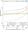 |
Fig. 4 Lyman-alpha and 1280 Å brightness curves of growth with |


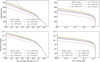 |
Fig. 5 Methane number density and mixing ratio profiles. The profile from Moses et al. (2018) is shown for reference only. All other profiles are calculated using Eq. (1). The profiles with solid lines for |


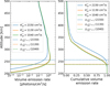 |
Fig. 6 Volume emission rate profiles at a solar zenith angle of 0◦ for Raman-scattered Lyα photons, i.e. photons scattered from Lyα to 1280 Å by H2. These photons can be scattered again by H2 (Rayleigh scattering at 1280 Å) and contribute to the 1280 Å brightness of Uranus. The solid lines in the left and right panels show the absolute and cumulative volume emission rates, respectively, for the Raman-scattered Lyα photons in atmospheres with the three best-fit methane profiles that reproduce the observed Raman feature brightness of |


5 Summary and conclusions
We analysed HST STIS and COS observations of Raman-scattered Lyα emissions of Uranus centred at 1280 Å, taken in 2012 and 2014, respectively. These emissions are observed at Uranus because of efficient Rayleigh–Raman scattering, resulting from the confinement of hydrocarbons, especially methane, at altitudes lower than those where significant Rayleigh–Raman scattering occurs. We estimate a brightness of  R for the 1280 Å feature from the STIS observations. This brightness value is consistent with that measured by Voyager 2 after considering recalibration by a factor of ∼0.5. Although the COS observations corroborate the STIS observed value, the brightness derived from COS is less certain. The HST STIS and COS observations confirm that this 1280 Å feature is persistent at Uranus, and detected at similar levels in 1986, 2012, and 2014.
Since methane absorbs far-ultraviolet radiation, the observed brightness of the Raman feature and Lyα emissions can be used to constrain the upper altitude region where CH4 is present in Uranus’ atmosphere. With this aim, we modelled the CH4 profile using Eq. (1). We did not consider hydrocarbon photochemistry in our modelling. For the remainder of Uranus’ atmosphere, we adopted the model that fits the 2011 HST STIS Lyα slitless spectroscopy observations presented in Joshi et al. (2025), with minor adjustments to the H densities. We also used the Lyα brightness of 725 ± 9 R derived by Joshi et al. (2025), because the 2012 STIS spectrum analysed in this study did not allow us to reliably estimate this brightness.
To derive the CH4 profile parameters from the Voyager 2 Raman feature observations, Yelle et al. (1987) did not consider resonant scattering, arguing that atomic H scatters Lyα photons only within the narrow region around the core of the broad solar Lyα line. When considering only Rayleigh–Raman scattering by H2 as done by Yelle et al. (1987), we obtain a similar eddy diffusion coefficient value to theirs for the CH4 profile that reproduces the observed 1280 Å brightness.
However, our results show that including resonant scattering by H significantly enhances the modelled 1280 Å brightness, even though this scattering occurs over a relatively narrow spectral region compared to continuous scattering by H2. The reason for this enhancement is an effective trapping of Lyα photons in Uranus’ extended hydrogen atmosphere because of highly efficient resonant scattering. This trapping increases Rayleigh– Raman scattering relative to the case without H resonant scattering, in which most photons pass through the upper atmosphere unscattered. When resonant scattering is included, the CH4 profile that fits the observed 1280 Å and Lyα brightnesses aligns better with other more recently published CH4 profiles and eddy diffusion coefficient values (Orton et al. 2014; Lellouch et al. 2015; Moses et al. 2018).
We achieved the observed Raman feature brightness of  R with CH4 profiles characterised by
  values ranging from 2150 cm2/s (yielding 14 R) to 1040 cm2/s (yielding 21 R). The resulting profiles indicate that CH4 number density falls below 1 cm−3 above altitudes between approximately 478 and 515 km (pressure of 4 × 10⁻³ to 2.4 × 10⁻³ mbar). The Lyα absorption optical depth reaches unity between altitudes of approximately 257 to 237 km (pressure of 1.65 × 10⁻¹ to 2.54 × 10⁻¹ mbar), which is below the peak Rayleigh–Raman scattering altitude or pressure region (see Fig. 6), resulting in the formation of this unique feature at Uranus among the Solar System’s giant planets.
The main conclusion of Yelle et al. (1987) was that at Uranus, Kzz is several orders of magnitude lower than on other planets, indicating that the methane homopause is at a pressure several orders of magnitude higher than on other planets. Our results corroborate this conclusion. We note that because we do not include photochemistry in our modelling, our values of  are likely underestimated. Nevertheless, our estimates of the methane depletion altitude and corresponding pressure provide an independent and crucial input for detailed photochemical models. These findings also highlight the importance of a UV instrument on the future Uranus Orbiter and Probe (UOP) mission. Such an instrument, with higher sensitivity and spectral resolution, could also observe rotational Raman lines branching from Lyα. This would enable a more precise estimation of the methane depletion altitude and the associated photochemistry. Methane profiles have been estimated to vary across the planet (see, e.g. Moses et al. 2018). Therefore, multipoint measurements of Raman-scattered Lyα emissions at Uranus could help constrain the spatial variation of CH4 across the planet.
Acknowledgements
Sushen Joshi, Lorenz Roth, and Nickolay Ivchenko acknowledge support from the Swedish National Space Agency through PhD grant 187/20. Jean-Yves Chauffray and Laurent Lamy acknowledge support from CNES and CNRS/INSU national programs of planetology (PNP) and helio-physics (PNST, also funded by Onera). We thank Julie Moses for the discussion/suggestions on methane profile modelling. Finally, we thank Prof. Roger Yelle for his review, which helped to improve the manuscript. This work is based on observations of the NASA/ESA HST programs GO 13012 and 14036, accessible through the MAST archive at http://mast.stsci.edu/ and the APIS service http://apis.obspm.fr.
References
- Atreya, S. K., & Ponthieu, J. J. 1983, P & SS, 31, 939 [Google Scholar]
- Barthélemy, M., Lamy, L., Menager, H., et al. 2014, Icarus, 239, 160 [CrossRef] [Google Scholar]
- Bishop, J., Atreya, S. K., Herbert, F., & Romani, P. 1990, Icarus, 88, 448 [Google Scholar]
- Brandt, J. 1963, P & SS, 11, 725 [Google Scholar]
- Broadfoot, A. L., Herbert, F., Holberg, J. B., et al. 1986, Science, 233, 74 [NASA ADS] [CrossRef] [Google Scholar]
- Broadfoot, A. L., Atreya, S. K., Bertaux, J. L., et al. 1989, Science, 246, 1459 [NASA ADS] [CrossRef] [Google Scholar]
- Burgdorf, M., Orton, G., van Cleve, J., Meadows, V., & Houck, J. 2006, Icarus, 184, 634 [NASA ADS] [CrossRef] [Google Scholar]
- Carlson, R. W., & Judge, D. L. 1971, P & SS, 19, 327 [Google Scholar]
- Chandrasekhar, S. 1960, Radiative Transfer (New York: Dover Publications), 393 [Google Scholar]
- Clarke, J. T., Durrance, S., Atreya, S., et al. 1986, JGR: Space Phys., 91, 8771 [Google Scholar]
- Feautrier, P. 1964, C. R. Acad. Sci. Paris, 258, 3189 [Google Scholar]
- Flasar, F. M., Conrath, B. J., Gierasch, P. J., & Pirraglia, J. A. 1987, JGR: Space Phys., 92, 15011 [Google Scholar]
- Ford, A. L., & Browne, J. C. 1973, At. Data Nucl. Data Tables, 5, 305 [Google Scholar]
- Gladstone, G. R. 1982, J. Quant. Spectrosc. Radiat. Transf., 27, 545 [Google Scholar]
- Gladstone, G. R., Pryor, W. R., & Alan Stern, S. 2015, Icarus, 246, 279 [NASA ADS] [CrossRef] [Google Scholar]
- Herbert, F., & Hall, D. T. 1996, JGR: Space Phys., 101, 10877 [Google Scholar]
- Herbert, F., & Sandel, B. R. 1999, P & SS, 47, 1119 [Google Scholar]
- Herbert, F., Sandel, B. R., Yelle, R. V., et al. 1987, JGR: Space Phys., 92, 15093 [Google Scholar]
- Herzberg, G. 1950, Molecular Spectra and Molecular Structure: Spectra of Diatomic Molecules (New York: D. Van Nostrand Reinhold Company) Jenkins, E. B. 1969, Icarus, 10, 379 [Google Scholar]
- Joshi, S., Roth, L., Gladstone, R., et al. 2025, A&A, 693, A231 [NASA ADS] [CrossRef] [EDP Sciences] [Google Scholar]
- Karkoschka, E., & Tomasko, M. 2009, Icarus, 202, 287 [NASA ADS] [CrossRef] [Google Scholar]
- Koskinen, T. T., Sandel, B. R., Yelle, R. V., et al. 2015, Icarus, 260, 174 [NASA ADS] [CrossRef] [Google Scholar]
- Lellouch, E., Moreno, R., Orton, G. S., et al. 2015, A&A, 579, A121 [NASA ADS] [CrossRef] [EDP Sciences] [Google Scholar]
- Lindal, G. F., Lyons, J. R., Sweetnam, D. N., et al. 1987, JGR: Space Phys., 92, 14987 [Google Scholar]
- Marrero, T. R., & Mason, E. A. 1972, JPCRD, 1, 3 [Google Scholar]
- Moses, J. I., Fletcher, L. N., Greathouse, T. K., Orton, G. S., & Hue, V. 2018, Icarus, 307, 124 [Google Scholar]
- Orton, G. S., Moses, J. I., Fletcher, L. N., et al. 2014, Icarus, 243, 471 [Google Scholar]
- Pearl, J. C., Conrath, B. J., Hanel, R. A., Pirraglia, J. A., & Coustenis, A. 1990, Icarus, 84, 12 [NASA ADS] [CrossRef] [Google Scholar]
- Quémerais, E., Sandel, B. R., Izmodenov, V. V., & Gladstone, G. R. 2013, in Cross-Calibration of Far UV Spectra of Solar System Objects and the Heliosphere, eds. E. Quémerais, M. Snow, & R.-M. Bonnet, ISSI Scientific Report Series (New York, NY: Springer), 141 [Google Scholar]
- Roman, M. T., Banfield, D., & Gierasch, P. J. 2018, Icarus, 310, 54 [NASA ADS] [CrossRef] [Google Scholar]
- Roman, M. T., Fletcher, L. N., Orton, G. S., Rowe-Gurney, N., & Irwin, P. G. J. 2020, AJ, 159, 45 [NASA ADS] [CrossRef] [Google Scholar]
- Sandel, B. R., Shemansky, D. E., Broadfoot, A. L., et al. 1979, Science, 206, 962 [Google Scholar]
- Sandel, B. R., Shemansky, D. E., Broadfoot, A. L., et al. 1982, Science, 215, 548 [Google Scholar]
- Scharmer, G. B., & Nordlund, Ã. 1982, Stockholms Observatoriums Reports, 19 [Google Scholar]
- Schunk, R., & Nagy, A. 2009, Ionospheres: Physics, Plasma Physics, and Chemistry, 2nd edn., Cambridge Atmospheric and Space Science Series (Cambridge: Cambridge University Press) [Google Scholar]
- Sromovsky, L. A., Karkoschka, E., Fry, P. M., et al. 2014, Icarus, 238, 137 [NASA ADS] [CrossRef] [Google Scholar]
- Sromovsky, L. A., Karkoschka, E., Fry, P. M., de Pater, I., & Hammel, H. B. 2019, Icarus, 317, 266 [NASA ADS] [CrossRef] [Google Scholar]
- Strobel, D. F., Yelle, R. V., Shemansky, D. E., & Atreya, S. K. 1991, The upper atmosphere of Uranus (Tucson: University of Arizona Press) [Google Scholar]
- Vatsa, R. K., & Volpp, H. R. 2001, Chem. Phys. Lett., 340, 289 [NASA ADS] [CrossRef] [Google Scholar]
- Yelle, R. V., Doose, L. R., Tomasko, M. G., & Strobel, D. F. 1987, GRL, 14, 483 [NASA ADS] [CrossRef] [Google Scholar]
- Yelle, R. V., McConnell, J. C., Strobel, D. F., & Doose, L. R. 1989, Icarus, 77, 439 [NASA ADS] [CrossRef] [Google Scholar]
Appendix A Details of the radiative transfer simulations
We adapted the REDISTER resonance line code described in Gladstone (1982) to perform the scattering calculations presented in this paper. For each atmosphere model, we performed two simulations. The first simulation (Lyα run) calculated the Lyα radiation field, with simultaneous resonant scattering by H and Rayleigh scattering by H2 (and absorption by CH4). Solar Lyα radiation was the external source for this run, and we represented the solar Lyα line profile by summing two equal and offset Gaussians with two equal and offset Lorentzians, as described by Gladstone et al. (2015). We did not consider attenuation of the solar Lyα line by the interplanetary hydrogen, with the same argument as we present in Appendix B of Joshi et al. (2025). Assuming the Lyα line to be symmetric, we used a one-sided logarithmic wavelength grid (based on Scharmer & Nordlund (1982)), with 18 wavelengths from line-centre (i.e. 1215.67 Å) out to 100 Doppler units (at a reference temperature of 200 K), or 0.74 Å, with wavelength bin sizes from 1.78e-3 Å at line-centre up to 5.2e-1 Å in the distant line wing.
In the Lyα run, for each scattering event of a Lyα photon by H2, we considered ‘branching’ fractions of 0.86, 0.055, and 0.086 (summing to unity) for the fraction of scattered photons either 1) remaining at Lyα (Rayleigh-scattered), 2) jumping via rotational Raman transitions to wavelengths near Lyα, or 3) jumping to 1280 Å via the vibrational Raman transition, respectively, using cross-sections given by Ford & Browne (1973). The Rayleigh-scattered photons can then potentially contribute to the Lyα brightness of Uranus. We neglected the rotational Raman-scattered photons from any further calculations. We calculated the volume emission rate profile of 1280 Å vibrational Raman-scattered photons. Using this volume emission rate profile as an internal source for the identical atmosphere model as for the Lyα run, we performed a second simulation (Raman run).
In the Raman run, we calculated the H2 Rayleigh scattering of this internal source of 1280 Å photons (that were branched from the Lyα photons in the Lyα run) while considering the absorption by CH4. We did not consider the Raman scattering of 1280 Å photons back to the original (Lyα) line in these calculations (an anti-Stokes process, cf. Herzberg (1950)), as that would require scattering by H2 molecules that are vibrationally excited (e.g. H2 (v=1)), and it was expected that these would be in short supply on Uranus (at least, away from strong auroras).
We considered angle-averaged partial frequency redistribution for Lyα resonant scattering by H (in the Lyα run). However, for the scattering calculations of Raman-scattered photons in the Raman run, we only considered monochromatic Rayleigh scattering by H2 at 1280 Å. Furthermore, due to the limitations of the REDISTER code, we approximated true Rayleigh scattering by isotropic scattering using the Rayleigh cross-section, which likely introduces an error of ∼10% (cf. Chandrasekhar (1960)). For both the runs, the model considers a 1D plane-parallel atmosphere, and we ran it for multiple solar zenith angles. Inside the atmosphere, scattering of photons is solved using Feautrier’s method (Feautrier 1964). For each solar zenith angle, the after-scattering source functions and extinctions are calculated for each atmospheric level. The after-scattering source functions and extinctions (from multiple solar zenith angle runs) are then interpolated along the lines of sight of interest, with proper accounting for sphericity, to calculate the emergent radiation from Uranus’ atmosphere by the formal solution of the radiative transfer equation. Taking into account the solar phase angle, we considered the entire planetary disk to obtain the average Lyα and Raman disk brightness through these calculations.
Appendix B Altitude versus pressure in the model atmosphere
Figure B1 shows the altitude versus pressure profile in our model atmosphere, for the easier comparison of our results with other studies.
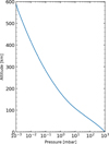 |
Fig. B1 Altitude versus pressure in the model atmosphere used in this study. |
All Tables
All Figures
|
Fig. 1 Uranus as observed from Earth during the Voyager 2 flyby (left) and 2012 HST STIS observations (right). The orange lines indicate the STIS slit orientation with respect to Uranus’ disc. |
| In the text | |
|
Fig. 2 Observations of Uranus with HST/STIS, using the G140L grating and 0.5″-wide slit separate emissions at the vibrational Raman branch around 1280 Å from other Uranus and geocorona emissions. The upper panel shows the spectral flux (averaged over the spatial y-axis) as a function of wavelength. The bottom panel shows the wavelength-integrated brightness in Rayleigh along the slit. The average emission on Uranus’ disc (light blue shading) is 25.5 R. An average background of 5.5 R was measured away from the disc in two regions (shaded grey) along the slit. |
| In the text | |
|
Fig. 3 Spectral region around 1280 Å in HST/COS exposure taken with the G140L grating on November 2, 2014. All flux within the vertical dotted lines was integrated to extract the 1280 Å brightness feature. The dashed line shows a linear fit to the adjacent spectral regions used to correct for background emissions. |
| In the text | |
|
Fig. 4 Lyman-alpha and 1280 Å brightness curves of growth with |
| In the text | |
|
Fig. 5 Methane number density and mixing ratio profiles. The profile from Moses et al. (2018) is shown for reference only. All other profiles are calculated using Eq. (1). The profiles with solid lines for |
| In the text | |
|
Fig. 6 Volume emission rate profiles at a solar zenith angle of 0◦ for Raman-scattered Lyα photons, i.e. photons scattered from Lyα to 1280 Å by H2. These photons can be scattered again by H2 (Rayleigh scattering at 1280 Å) and contribute to the 1280 Å brightness of Uranus. The solid lines in the left and right panels show the absolute and cumulative volume emission rates, respectively, for the Raman-scattered Lyα photons in atmospheres with the three best-fit methane profiles that reproduce the observed Raman feature brightness of |
| In the text | |
|
Fig. B1 Altitude versus pressure in the model atmosphere used in this study. |
| In the text | |
Current usage metrics show cumulative count of Article Views (full-text article views including HTML views, PDF and ePub downloads, according to the available data) and Abstracts Views on Vision4Press platform.
Data correspond to usage on the plateform after 2015. The current usage metrics is available 48-96 hours after online publication and is updated daily on week days.
Initial download of the metrics may take a while.