| Issue |
A&A
Volume 705, January 2026
|
|
|---|---|---|
| Article Number | A220 | |
| Number of page(s) | 16 | |
| Section | The Sun and the Heliosphere | |
| DOI | https://doi.org/10.1051/0004-6361/202556890 | |
| Published online | 20 January 2026 | |
Toward solar many-line inversions of high-resolution spectropolarimetric data
1
Max-Planck-Institut für Sonnensystemforschung Justus-von-Liebig-Weg 3 37077 Göttingen, Germany
2
Thüringer Landessternwarte Sternwarte 5 07778 Tautenburg, Germany
3
Big Bear Solar Observatory, New Jersey Institute of Technology 40386 North Shore Lane Big Bear City CA 92314, USA
4
Center for Solar-Terrestrial Research, New Jersey Institute of Technology Newark 07102-1982 NJ, USA
5
Astronomy Program, Department of Physics and Astronomy, Seoul National University, 1 Gwanak-ro Gwanak-gu Seoul 08826, Republic of Korea
6
Korea Astronomy and Space Science Institute, 776 Daedeok-daero Yuseong-gu Daejeon 34055, Republic of Korea
★ Corresponding author: This email address is being protected from spambots. You need JavaScript enabled to view it.
Received:
18
August
2025
Accepted:
24
November
2025
Abstract
Context. For the analysis of highly resolved solar spectra the simultaneous observation and interpretation (inversion) of only a few (often only one) spectral lines is still the norm. With modern instruments spatially highly resolved spectropolarimetric data covering many lines are available.
Aims. For the first time we combine the information from 85 simultaneously observed absorption lines in spatially highly resolved data to test a proposed solar many-line inversion strategy.
Methods. We inverted full Stokes spectra recorded with the FISS spectro-polarimeter (FISS-SP) at the 1.6-m Goode Solar Telescope in California, using the SPINOR code. We contrasted two different setups: one following the traditional approach of using a line doublet, and a new method inverting many-lines simultaneously.
Results. Compared to results from an inversion using two lines of a line doublet, we discovered more fine-structure and better constrained values using the many-line technique. An average quiet Sun spectrum was successfully reproduced using a model atmosphere, but when inverting spatially resolved data, uncertainties in line parameters and blend configurations did not average out. Thus, a deliberate selection process of lines and line blends was required, in order to make the many-line case converge to a physically expected and coherent atmosphere. We successfully developed and tested such a selection method.
Conclusions. Our results highlight that the many-line inversions method delivers more coherent results with superior line of sight (LOS) resolution of the atmospheric structure. Moreover, it effectively detects and utilizes even weak polarimetric signals in noisy data and thereby partly circumvents low noise requirements. It reveals uncertainties in atomic parameters of individual spectral lines and models, as the degree of freedom to compensate for these uncertainties by compromising the inferred atmospheric parameters is considerably reduced. It is thereby pointing to a need for improved atomic data, including log(gf) values, of many lines in the solar spectrum. The many-line method presents significant potential for solar physics and may become the preferred option for future observations with upcoming spectrographs.
Key words: methods: numerical / methods: observational / Sun: photosphere
© The Authors 2026
 Open Access article, published by EDP Sciences, under the terms of the Creative Commons Attribution License (https://creativecommons.org/licenses/by/4.0), which permits unrestricted use, distribution, and reproduction in any medium, provided the original work is properly cited.
This article is published in open access under the Subscribe to Open model.
Open access funding provided by Max Planck Society.
1. Introduction
To comprehend the solar lower atmosphere, it is essential to discern its physical features, most notably the temperature (T), the line-of-sight velocity (vLOS), and the magnetic field defined by its strength (B), azimuth (ϕ), and inclination (γ). The most effective way of determining these characteristics from the observed polarization profiles is the application of Stokes inversions, which leads to the creation of a model atmosphere that can accurately represent the observations, within the model’s assumptions and constraints.
In contrast to stellar physics, for the analysis of solar spectra, the simultaneous observation and inversion of only a few spectral lines is still the norm. One reason for the limitation to a few lines is the preference for isolated, not blended, spectral lines embedded in a distinct continuum, which simplifies the calibration and inversion processes. In addition, in solar observations, much effort is invested in imaging and capturing the fast evolution of the solar scene, which necessitates fast data retrieval. This can be accomplished by reducing the number of pixels to be read out from a sensor. This can be done by restricting the field of view (FOV) or the wavelength range; the choice is typically to limit the wavelength range. Hence, the use of many lines simultaneously has mostly been limited to the analysis of spatially low-resolution data from Fourier transform spectrometers (FTS, Brault 1978).
To achieve the required high polarimetric sensitivity, measurements need to have a high resolution in the spatial, spectral, and temporal domains, paired with a low noise level. Ideally, the noise should be between 10−3 and 10−5 of the continuum intensity (See Iglesias et al. 2016, and references therein). Another way to reach the sensitivity goal is to use the signal from many spectral lines. In the era of fast large format imaging sensors and improved data handling capabilities, the need to observe only a few lines is no longer so strong. Consequently, Riethmüller & Solanki (2019) suggested exploring the merits of using many absorption lines simultaneously. They showed that the outcomes from the many-line (ML) inversion were more precise and more robust against noise.
The diffraction-limited data from FISS-SP (van Noort et al. 2025), the spectropolarimetric extension of the Fast Imaging Solar Spectrograph (FISS, Chae et al. 2013), installed at the 1.6-meter Goode Solar Telescope (GST, Goode et al. 2010; Cao et al. 2010; Goode & Cao 2012) at the Big Bear Solar Observatory (BBSO) exceeds a spectral range of 30 Å and covers 171 relevant absorption lines. It is, therefore, particularly suited for such a many-line inversion technique. In this study, we present the first application of the many-line inversion method to spatially highly resolved solar observations and compare it with a traditional inversion approach using a line doublet. We further discuss the necessity of, and a strategy for, the selection of lines for such a many-line inversion.
2. Forward challenges and inversion problems
To appreciate the benefits and understand the challenges of solar many line inversions better, it is essential to remind ourselves of some inherent complications of the Stokes inversion process. The core of a Stokes inversion is the numerical solution of the differential radiative transfer equation (RTE). If the properties of the solar atmosphere, notably temperature, velocities, and magnetic field, are known, and local thermal equilibrium (LTE) can be assumed, the solution is relatively simple and results in synthetic I, Q, U, V-Stokes profiles for selected line(s). Unfortunately, for spectropolarimetric observations the opposite is true: The Stokes profiles are known and the configuration of the solar atmosphere is the unknown parameter. The extraction of an descriptive atmospheric model is typically accomplished by iterative modifications to the assumed configuration, re-calculating the corresponding Stokes profiles, and minimizing the difference to the observed profiles (del Toro Iniesta & Ruiz Cobo 2016).
Unfortunately, multiple atmospheric configurations can result in identical profiles. Moreover, as we can only observe the integral over the optical depth along the viewing angle, traces from different heights might cancel out or leave only a fuzzy footprint in the profiles. This degeneracy renders it impossible to derive the complete and turbulent stratification from observational data. Nonetheless, by employing physical assumptions and using a microturbulence factor to account for the fuzzy broadening, the extraction of stratified information is possible (see, for instance, Frutiger et al. 2000; Danilovic et al. 2016; Milić & van Noort 2018; de la Cruz Rodríguez et al. 2019; Ruiz Cobo et al. 2022; Castellanos Durán et al. 2024), although incomplete. The inversion problem can usually be further constrained with the full set of Stokes parameters, but this constraint is still not perfect. For instance, the impact of even relatively strong horizontal fields on Q, U, or V signals can be very small. The response of the line to a change in the atmospheric configuration is interconnected to the formation height of its core and wings, as outlined in Smitha et al. (2020). Using many lines, formed at different heights, hence adds constraints at those heights allowing the atmospheric stratification to be more clearly discerned (See, for instance, Sütterlin et al. 1996; Riethmüller & Solanki 2019).
A crucial ingredient for the success of a Stokes inversion is the knowledge of the atomic parameters of the observed spectral lines. Factors such as the excitation potential of the transition’s lower energy level, the central wavelength of the spectral line, and the weighted oscillator strength, typically given as log(gf), significantly impact the line shape and depth. Not all of these parameters of all spectral lines of interest are known with the necessary accuracy from laboratory experiments (Borrero et al. 2003). The effects of a line being in LTE or not (non-LTE, NLTE) can influence the result of an inversion in a similar way (see, Shchukina & Trujillo Bueno 2001; Borrero & Bellot Rubio 2002; Smitha et al. 2020, 2021). In addition, the influence of 3D NLTE and radiative transfer effects on line profiles becomes increasingly relevant, the higher resolution of the observation is Holzreuter & Solanki (2012, 2013, 2015). Since atomic parameters and atmospheric configuration both influence the line profile, poorly determined parameters and incomplete models might lead to accurate fits of an observed profile, but the inferred parameters then might not represent the actual atmosphere. From only a single spatial pixel and spectral line, it is comparatively difficult to affirm the accuracy of the line parameters.
Lastly, observational data is never ideal or perfect. Most notably the inevitable noise hides subtle signals in the observed profiles and increases the range of profiles considered to be a “good fit”. This results in a further degradation of the already complex inversion problem (van Noort 2012; Danilovic et al. 2016). Moreover, observational data is naturally limited in resolution and available photons and some spatial- and temporal averaging is inevitable. Recently, Sinjan et al. (2024) showed that this can lead to an underestimation of the magnetic flux everywhere on the solar disk.
All these factors affect each other in a complex and nonlinear way, making the inversion of observational profiles a highly degenerate problem. The work by Riethmüller & Solanki (2019) indicated that the consolidated signal of multiple lines can alleviate some of these issues. Also Díaz Baso et al. (2025) found it beneficial to use multiple lines to counteract spectral degradation and noise. Vukadinović et al. (2024) devised a method to refine atomic parameters, for example log(gf), by combining information from multiple spectral lines and atmospheric configurations. However, all these studies used observables synthesized from numerical simulations, which circumvents some of the challenges when dealing with observations, highlighted above. In this study we test the performance of many-line inversions on highly resolved solar observations.
3. Observations and data calibration
For this study we used a scan acquired with the slit-scanning spectrograph FISS covering a spectral range of 33.06 Å. By making use of a polarimetric modulation package, resulting in a setup referred to as FISS-SP, all four Stokes parameters could be recorded. For further instrumentation details, please refer to van Noort et al. (2025).
The observation of an emerging active region was recorded at μ = 0.81 (cosine of the heliocentric angle) on May 11th, 2023, at 17:01 (UTC). The region was later assigned NOAA active region number AR 13 304. For this study, we used a small region of interest (ROI) from the available data, which had a good representation of different types of solar features. Figure 1 shows a continuum image extracted from the restored scan. The ROI used here is indicated with a blue box. Throughout the data reduction process, we followed the steps from van Noort et al. (2025). The spectroflat algorithm (Hölken et al. 2024) allows for an accurate and field-dependent correction of the spectral curvature effect, which is crucial for our goal of using absorption lines from the full spectral field of view. We used the Kitt Peak FTS solar atlas (Neckel 1999) to perform the wavelength calibration and also to set up the accurate wavelength scale on the averaged flat-field measurement that was closest in time, using the atlas-fit routine (Hölken et al. 2024). Based on a comparison with the FTS atlas we estimated and corrected for a gray spectral stray light level of 2.5%.
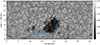 |
Fig. 1. Continuum image of the observed active region extracted from the restored scan. The scan direction is from top to bottom along the y-axis, the axis labels are in arcseconds, the intensity is normalized to I/IC. The blue box indicates the ROI used for this study; the black arrow indicates the direction to the disk center. |
The applied specrestore algorithm (van Noort 2017) solves for the undegraded image using the seeing related point spread function (PSF) contribution to each pixel as determined from a simultaneously recorded set of context images. In doing so, it not only improves the contrast and resolution, but also reduces the spatial stray light contribution to each pixel (van Noort 2012, 2017; van Noort & Doerr 2022). After reconstruction the data show a noise level of about one percent in all parameters, which is comparable with other reconstructed or deconvolved datasets (see van Noort & Doerr 2022, for a discussion). Unfiltered deconvolution is a linear operation that effects noise and signal in the same way. It therefore cannot change the signal to noise ratio (S/N). The Lucy-Richardson deconvolution algorithm used here only amplifies spatial frequencies below the diffraction limit and therefore acts as a filter to frequencies where there is only noise and no signal. Thus, the S/N of the restored data is enhanced (Barnes 2004; van Noort et al. 2025), compared to the original data.
After reconstruction we estimated the residual unpolarized wide-field spatial stray light, that cannot be removed by deconvolution. For this we spatially averaged over the quiet part of the scan and subtracted the resulting profile weighted by a number < 1, from the umbral profiles. After subtracting 15% of this averaged quiet-Sun line profile, the intensity in the cores of the strongest lines in the umbra becomes negative, producing a hard upper limit for the residual spatial stray light. As there are no means to estimate a lower limit in a similar way and the stray light must be below 15%, we decided to not correct for the residual wide field stray light.
As described in van Noort et al. (2025), there is a variation of the PSF along the wavelength dimension in the FISS-SP data. The SPINOR inversion code (Frutiger 2000; Frutiger et al. 2000) assumes the same instrumental broadening for all lines. To allow for a simultaneous inversion of the complete spectral range, a homogenization of the spectral PSF was applied. For this we convolved the recorded spectra with a Gaussian that had a spatially varying full width at half maximum (FWHM). The effective differential FWHM was determined for each wavelength position by the difference between the FWHM of the widest part of the spectral PSF and the FWHM at the given wavelength position.
4. Inversion setup
The spectrum in the observed 5250 Å region is dominated by iron, titanium, vanadium, and chromium. Table 1 provides an overview of the 171 main contributors to the absorption spectrum and the used relative abundances of the respective elements. The line information was collected from the Kurucz line list (Kurucz et al. 2009; Kurucz 2018) and the Vienna Atomic Line Database (VALD, Ryabchikova et al. 2015; Pakhomov et al. 2019). In the few cases of discrepancies where none of the parameters could sufficiently reproduce the lines we manually adjusted the log(gf) until the discrepancy was minimal on multiple selected reference pixels (Compare, Vukadinović et al. 2024). The abundances are based on Asplund et al. (2021).
Number of relevant solar absorption lines per element and ionization state.
Riethmüller & Solanki (2019) have demonstrated the general suitability of SPINOR for the inversion of spatially resolved many-line observations. In a pixel-by-pixel inversion approach, information from neighboring pixels is not utilized. As discussed in Section 2, observed spectra can sometimes be reproduced by different atmospheric configurations without significantly affecting the χ2 values of the pixel. This could lead to a large variance in the fitted parameters of adjacent spatial pixels, even though these contain information from essentially the same resolution element. To avoid this salt-and-pepper type noise and to converge into consistent maps of a spatially extended FOV, some form of spatial regularization is necessary. Intrinsically, SPINOR inverts all pixels independently. To use the information from adjacent pixels, we applied Gaussian smoothing to the maps resulting from a given SPINOR execution, and applied filters to the maps of the inclination and azimuth to keep them within the ± 90° range. We then restarted the inversion process with the smoothed maps as improved initial estimates (van Noort 2012; van Noort et al. 2013). In this article, we use the term “iterations” to describe the number of optimization steps SPINOR uses to fit a single pixel profile, and “cycles” for the repeated runs of the SPINOR code with improved initial estimates introduced between them.
To verify the setup of the inversion and the atomic line parameters in use, we replicated the spectrum of an averaged FISS-SP flat-field measurement with the Harvard-Smithsonian reference atmosphere (HSRA) (Gingerich et al. 1971), utilizing the strongest 171 absorption lines within the spectral window of the dataset (Table 1). The average of the flat-field measurement is particularly suitable for this exercise as it is recorded in the quiet Sun at disk center and thus represents an averaged atmosphere, similar to the HSRA model. We adjusted the temperature offset to match the continuum levels of the synthetic spectrum with the observed one and further allowed the code to fit a height dependent microturbulence term, while all other values are taken from HSRA. The result is shown in Figure 2.
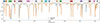 |
Fig. 2. Comparison of the computed spectrum using the HSRA model with a normalized Stokes I profile from an averaged FISS-SP flat-field measurement. We allowed the code to adjust for microturbulence and temperature offset. The bar above the profile indicates the spectral windows R01–R18 from Table 2. |
4.1. Spatially resolved convergence challenges
We found it almost impossible to make the code converge to a consistent and physical solution when inverting the complete line list simultaneously on high spatial resolution spectra. For instance, we commonly found unrealistically high field values in the centers of granular cells, an unrealistic flow stratification, or strong inter-parameter cross-talk. Even though we were able to reproduce the average spectrum with a slightly adjusted HSRA model, we were not able to extract a physically meaningful spatially resolved atmosphere from those lines. While in average quiet Sun profiles, magnetic field and velocities are negligibly small, this might not be the case in better resolved spectra.
We tested different node setups, including number and position, to account for the higher complexity of the spatially better resolved data, but none of them showed a significantly better fit quality nor an atmosphere that would consistently match our expectations. We finally adopted the configuration reported to be optimal by Danilovic et al. (2016) and placed three height nodes at optical depth of log(τ) := log(τ5000 Å) ∈ {−2.0, −0.8, 0.0}. As atmospheric model we choose the established setup (Riethmüller et al. 2008; van Noort 2012; Castellanos Durán et al. 2024) with height dependent temperature, magnetic field strength, LOS velocity, and microturbulence, whereas field inclination and azimuth angle are assumed to be height-independent.
With this setup we could trace the issues with the resulting atmosphere to the selection of lines, by inverting the data using only the 5247/5250 Fe I spectral lines. The result was noisy and imperfect, but matched our general expectations for the selected solar scene (details are given in Section 5.1). Expanding the line list again soon led to the known issues of atmospheric configurations outside the physical expectations. A careful examination of the lines, weights, and spectral windows and their influence on the inversion result was thus necessary. Facing similar challenges when analyzing stellar spectra, Bigot & Thévenin (2006) and Heiter et al. (2021) compiled lists of “well-behaved” spectral lines that have well established atomic parameters and do not show anomalous behavior. Laverick (2019) compared a large number of line parameters from many different databases to remove systematic errors in the atomic data. They report that less than 40% of the assessed Fe I lines had sufficiently accurate log(gf) -values. However, all these lists focus on nonblended lines and are much too sparse for our endeavour. Therefore, we decided to try to identify problematic lines in our observed spectral region ourselves. Unfortunately, simply ignoring spectral lines that are present in the observation but which are not modeled by the inversion code, has a negative impact on the deduced atmosphere as well. To exclude such a line, we must exclude it from the fit, which is accomplished most conveniently by splitting the spectrum into discrete spectral windows.
We selected 18 such windows using the following three criteria: (1) The selected spectral window is free from lines that could not be reproduced by our code, (2) a section of continuum is present in the window, and (3) the lines within a spectral window need to provide enough information to constrain the target atmospheric stratification on their own.
Overview of the 18 spectral windows.
In areas with large velocities the spectral profiles are strongly shifted. If this shifts a spectral line or an undescribed blend from a wavelength window with a strongly negative influence on the inversion result into (one of) the spectral window(s), the inversion result, again, suffers from the fact that this part of the spectrum, that should be excluded, is now being inverted. To mitigate this problem, the offending part of the spectrum must be either generously clipped or the border(s) of the spectral window(s) must be shifted on a per-spatial-pixel-basis according to the velocities (once known). We used the conservative first approach to avoid further complications in the comparison of the results. For regions with strong lines that have a high effective Landé-g∗-factor (Shenstone & Blair 1929) we have chosen higher weights on Stokes V, as the determination of the magnetic field from V is less affected by residual wide-field stray light, which is unlikely to be polarized. We then individually inverted all 18 spectral windows independently from each other. Table 2 lists the spectral windows and included species that we used from our dataset. The full set of atomic line parameters and weights used can be found in Appendix A.
4.2. Selection of spectral windows
From the corresponding intensity image, we identified four atmospheric features, namely granules, intergranular lanes, umbra and umbral dots. Figure 3 shows, for each of these four types of atmospheric features, the values of the atmospheric parameters temperature, line-of-sight velocity and magnetic field strength, given at the three height nodes used for the inversion. The individual symbols represent the mean values obtained from each of the 18 wavelength windows listed in Table 2. The error bars indicate standard deviation of the extracted atmospheric parameters per optical depth node.
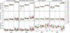 |
Fig. 3. Comparison of atmospheric parameters deduced from the 18 selected spectral windows (see Table 2), separated by type of solar feature. The main columns show properties of granules, inter-granular lanes, bright points, umbra, and umbral dots. Each column is sub-divided by dashed lines into the values of the parameters at the different optical depth nodes. Each row refers to one atmospheric parameter (temperature, LOS velocities, and field strength). Each spectral window is represented by a symbol, indicating the mean value of the retrieved parameter from all pixels corresponding to the given physical parameter, and a range bar, indicating the standard deviation. The excluded windows are marked with an ×-symbol. The gray entry indicates the mean of the finally used 14 spectral windows and the black entry the result from the simultaneous many-line inversion (see main text for a detailed discussion). |
While the results from most spectral windows align reasonably well, the variation in their sensitivity under different atmospheric conditions and at height nodes is apparent. R04, R05, and R11 all show strong deviations from the results obtained in the other windows in the vLOS and temperature, and we excluded these spectral regions from the final setup. The temperature at log(τ) = −2 of R09 also does not agree with the other spectral windows. However, since the temperature is generally so well constrained, we found that insensitivity to temperature in the higher nodes alone does not compromise the overall result when adding the corresponding lines to our many-line inversion setup.
The photospheric field strength needs a closer look, because we found that small deviations from the mean solution in this parameter have a strong influence on the combined solution. This is especially apparent for the weak fields commonly found in granulation. As this is barely visible in Figure 3, we provide a zoomed-in view of the corresponding panel in Figure 4. We found that the addition of regions R01 and R08 drives the extracted atmosphere to implausible regimes. The regions R03 and R15 also show stronger field values in the highest and lowest node respectively, but the addition of the corresponding lines had no negative effect on the result of the many-line inversion. Hence, we draw a line at approximately 650 G as the highest tolerable mean field value in granulation pixels. In Figure 4, we indicate this with a dotted horizontal line.
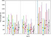 |
Fig. 4. Zoomed-in image of the lower left panel of Figure 3 (see legend in that figure) showing the field strength statistics for granular pixels. The threshold of (≈650 G) is highlighted with a dotted horizontal line. |
Figure 5 provides a typical example of a fit and corresponding stratification from the excluded spectral window R01. Here, the code identifies a solution with a strong magnetic field in the lower photosphere without significant signals in Stokes Q, U, and V. Given that this region contains two lines with an effective Landé-g∗-factor greater than 2.2, the catalyst for this solution could only be the near-continuum line broadening interpreted as a horizontal field. This solution is possible since the magnetic field is not sufficiently constraint from Stokes I alone and the noise in Stokes V allows this solution to satisfy the χ2 metric. The map of the magnetic field strength in the lowest optical depth node (panel f) shows many such field hot spots in the middle of a granule. For reference the profile and stratification according to the final many-line result (see Section 5) is included. The fit from the inversion of that region is a good representation of the observed line profile, while the profile synthesized from the atmosphere of the final result (ML-profile) diverges greatly. Additionally, the displacement of the ML-profile indicates disagreement in the line wavelength position between the set of lines used in the final setup and R01.
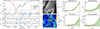 |
Fig. 5. Typical fit and stratification for the blended region R01 including ten spectral lines for a selected granulation pixel. Panels (a–d): Observation, and synthetic profiles in Stokes I, V, Q, and U in relative values of I. The R01 profile corresponds to the inversion result from the individual inversion of this region, while the ML profile was synthesized using the atmospheric configuration extracted from the many-line inversion result (see Section 5). Panels (e–f): Continuum image (e) of the granule with the selected pixel marked by the orange plus sign (+) and the corresponding map of the magnetic field strength (f) in the log(τ) = 0 node. Panels (g–j): Derived stratification for temperature (g), vLOS (h), turbulence (i) and field strength (j). The values at the log(τ ) nodes are indicated with a symbol, the line represents the spline fit. Orange is the stratification for the selected pixel from the inversion result, green shows the mean and range of the values from the green box indicated in the middle panel, and red shows the stratification for the many-line atmosphere of the selected pixel. |
The final line list consists of all regions from Table 2 that were not disregarded. Additionally, we added three weak lines on the red side of R11 and three other weak lines between regions R14 and R15. These lines could not be tested with the same setup as the other lines, as they do not constrain the atmospheric stratification in the middle or upper photosphere. Unfortunately, they are also separated from adjacent windows. However, these shallower lines help to constrain the parameters in the lower atmosphere, where the information can otherwise only be extracted from the wings of stronger lines. We have carefully tested the additional lines with a reduced setup without height resolution of magnetic field and velocities. We further compared the result before and after incorporating them into the full setup to ensure their compatibility.
In total we identified 85 solar absorption lines that do not show severe anomalous behavior. This set includes most of the stronger ones, distributed over 15 wavelength windows.
5. Results
As stated in van Noort et al. (2025) the average FISS-SP flat-field measurement reproduces the Kitt Peak FTS atlas well. During the setup we recreated the flat-field Stokes I spectrum using HSRA model for the dominant 171 absorption lines in our spectral window and achieved a good overall match with the temporally and spatially highly averaged profile. The result was presented in Figure 2. The use of the average quiet Sun spectrum allows us to connect to previous studies using multiple solar lines from spatially heavily averaged profiles, for instance Balthasar (1984), Solanki & Stenflo (1984, 1985), Allende Prieto et al. (1998), or Borrero & Bellot Rubio (2002).
Especially Fe I lines are typically weakened by overionization in non-LTE, and thus likely to have a somewhat too deep line-core when synthesized under the LTE assumption (Lites & Athay 1972; Rutten 1988; Solanki & Steenbock 1988). This effect is stronger the stronger the line. On the other hand, the HSRA model includes the temperature rise in the chromosphere. When synthesized in LTE, this causes the rest intensities in the cores of the deepest lines to be too high, which likely explains why the depths of the deepest 4 computed lines are almost exactly the same.
5.1. Fe line doublet inversions
To establish a link to other spatially extended inversion results, we treated the data in a well-tested manner: The Fe I doublet, consisting of the 5247.05 Å and the 5250.20 Å lines, is somewhat similar to the Fe I doublet at 6301.5 and 6302.5 Å observed by the spectropolarimeter on board the HINODE satellite (HINODE/SP, Lites et al. 2001; Kosugi et al. 2007; Tsuneta et al. 2008). Both lines of the 5250 Fe I doublet are within the spectral range of our dataset. Hence, we used a setup that was already successfully used many times for the inversion of HINODE/SP datasets (e.g., Riethmüller et al. 2008; van Noort 2012; van Noort et al. 2013; Castellanos Durán et al. 2024). With this, we inferred information on the physical parameters of the solar atmosphere including their height stratification. The result after 4 cycles of 75 iterations is shown in Figure 6.
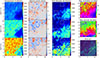 |
Fig. 6. Maps of the temperature, LOS velocities, and magnetic field strength at log(τ) ∈ {0.0, −0.8, −2.0}; and height independent inclination, azimuth, and χ2. This result is inferred with the traditional approach using the Fe I doublet that consists of the 5247.05 Å and the 5250.20 Å lines. We have used four cycles of 75 iterations each, the axis tick marks are in arcseconds (see main text for a discussion). In all figures negative vLOS denotes a flow toward the observer (i.e., up-flow) and positive LOS velocities denote a flow away from the observer (i.e., down-flow). |
The inferred maps feature salt-and-pepper type noise, especially in the higher temperature nodes and the azimuth and inclination of the magnetic field. Also immediately apparent is the missing granulation pattern in the low photospheric vLOS maps. Instead, the typical imprint of the granular and inter-granular flows can be found in the highest node at log(τ) = −2 only, which is higher than physically anticipated, but can be explained by the formation height of those lines. The lower two maps are dominated by patches that resonate between the two height nodes and other parameters, most prominently with the magnetic field strength. And also the maps of the magnetic field strength themselves prominently show voids (areas with apparently no field in a strong field regime, e.g. the umbra). We also observe the opposite: Areas with strong fields in a quiet region. These structures are almost always simultaneously present in multiple height nodes. We further refer to such cross-talk and void patches as areas with implausible values (AWIV). The fits, however, seem of a constant quality, as the corresponding χ2 map does not show the same structures. A typical example fit is presented in Figure 10.
The limited information on height stratification encoded within the 5250/5247 Fe I-line doublet is not unexpected. These lines are known to form at a very similar height and have therefore been prominently used by Stenflo (1973) to determine magnetic field values at their formation height. Even though the lines sample the entire atmosphere where they are formed, the sensitivity in the line wings is not enough to constrain the magnetic stratification in multiple height nodes in many pixels in our dataset. Together with the one percent noise level of the observation the height resolution that can be extracted from these two lines is limited. This is especially true for gradients which are determined by contrasting information from the line wings and line cores.
5.2. Many-line inversions
For the ML setup we simultaneously inverted all lines that could be identified as well behaved (see Section 4.2 and Appendix A). Figure 7 shows the inferred atmospheric configuration after two consecutive cycles of 75 iterations each on this setup. A third cycle was performed, but the differences to the previous result were negligible, so that we consider the inversion to be well converged.
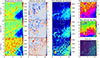 |
Fig. 7. Same as Figure 6, but for the final many-line setup using two cycles a 75 iterations and 85 lines. |
In the direct comparison of the atmospheres extracted using the traditional two line approach and the new many-line approach we find that the utilization of multiple lines with different formation heights, magnetic sensitivities, and responses is able to constrain the inversion problem better. While the general range of values in both setups match, the differences in the details are apparent. Compared to the result from the Fe I doublet, the new maps show the expected granular flows and, in all parameters, less salt-and-pepper type noise, even with only half as many cycles. In all maps, we notice a superior resolution of the fine structures. The maps of the azimuth and inclination of the magnetic field from the ML setup extend more coherent from the strong field into weak field regions.
Also in the ML approach we find AWIVs. However, here we find them mostly in the form of voids restricted to the highest node of the magnetic field map, which can mostly be explained by too steep gradients along the optical depth axis caused by the three node setup. Figure 8 presents a side-by-side comparison of some AWIVs from both setups. In the upper two panels we show typical examples of voids in the strong field regime of the umbra. The field gradient within the AWIV in the top left panel is reversed, suggesting that the signal required to constrain it is obscured by noise. In the corresponding ML columns not only the void is gone, but also more coherent fine-structure is visible. The weak field regions in the umbra of the many-line result can be associated with flows, for instance from umbral dots, which is expected (See for instance Schüssler & Vögler 2006; Riethmüller et al. 2008).
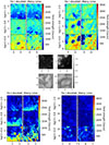 |
Fig. 8. Side-by-side comparison of magnetic field strength maps from both setups in four example areas. The continuum images in the middle panel correspond to the adjacent field maps panel. All tick marks are in arcseconds and within the reference frame of Figures 6 and 7 and are marked with white boxes therein. |
In the lower two panels we show typical examples from areas with weaker fields. In the left panel the (opposite) counterpart of a field void, an area with unexpected high field, is presented. In this case, the fitted profiles suggest that the code erroneously inferred a horizontal field from the noise present in the linear polarization profiles. This artifact is also not present in the atmosphere extracted with the ML setup. The lower right panel shows a granule with surrounding intergranular lanes. In the ML-case, we are presented with a well resolved smale-scale magnetic feature at the intersection of three intergranular lanes that can be associated with a bright point. In comparison only a fuzzy trace can be seen in the atmosphere extracted from two lines. In the ML case the combined information extracted simultaneously from many lines not only allows for a coherent height stratification and resolution of smale-scale events, it also eliminates most of the ambiguity in the profile which leads to these AWIVs.
Comparing the normalized χ2 maps we find that, in contrast to the more coherent atmosphere of the ML setup, the line doublet shows a better fit quality. This also holds when contrasting the fitted profiles directly. Figure 9 presents a typical fit for Stokes I, Q, U, and V from both setups and Figure 10 provides a zoom onto the two lines of the Fe I doublet to allow for a more detailed comparison of the fits.
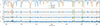 |
Fig. 9. Typical example of the observed and fitted profiles for both setups. The topmost panel shows Stokes I/IC while the other panels show relative signal strength of V, Q, and U respectively. IC corresponds to average quiet Sun continuum intensity. |
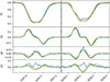 |
Fig. 10. Zoom in for Figure 9 on the two iron lines fitted in the traditional approach. Please refer there for legend. On this scale the difference in the fit quality, especially in I and Q becomes visible. We contribute the obvious discrepancy of both fits with Stokes U to residual, field depended, cross-talk from Stokes I in the data. |
6. Discussion
We noticed that in our case the inversion of the 5247/5250 Fe I line doublet does not readily lead to a coherent and physically meaningful model of the stratified solar atmosphere. This is possibly due to the relatively high noise level in the observations. When inverting our dataset with only those two spectral lines, spatial regularization, a reduced atmospheric stratification, or intense priming with expected values would have been necessary for the inversion code to converge further. A simplified inversion setup (e.g., Milne-Eddington) might have produced a better (albeit more restricted) result in the line-doublet case, but a too simple setup cannot account for the variety of lines used in the many-line inversion. On the other hand, the setup suggestion by Danilovic et al. (2016) strives to optimize the atmospheric model for a few-line inversion. In our many-lines case, a more complex model might be better suited, as indicated by Riethmüller & Solanki (2019). However, accounting for the noise in our dataset and in order to allow for a direct comparison of the two setups we have chosen the same atmospheric model for both inversions.
In the atmosphere inferred from the line doublet we find many areas where inter-node and inter-parameter crosstalk is apparent. Often these AWIVs feature sharp borders, where the atmospheric parameter is very different from one pixel to the other. These sharp features are stable over multiple inversion cycles and different initial guesses, indicating a converged solution. The corresponding χ2 map does not show the same structures and reports a similar fit quality inside and outside the AWIV. Hence, inside an AWIV a nonphysical atmosphere reproduces the spectral profile better than a physically expected one (see Section 2). Another example for the conflict of matching fit and physically expected atmosphere was presented in Figure 5.
In the ML case the combined information extracted simultaneously from many lines facilitates the resolution of smale-scale structures and allows for a spatially coherent height stratification. Especially, the typical noise-related AWIVs from the two line case are not present in the ML case. Combining many lines simultaneously allows signal that barely exceeds the noise floor to be reliably used (See, Figure 10), as the individual signals all constrain a common atmospheric property, which relaxes the low noise requirement for precise polarimetry. Utilizing lines that are diverse in formation height, Landé factor, excitation and ionization potential, and strength helps constrain all atmospheric parameters and their height stratification better, thus yielding a spatially smooth and physically more meaningful model of the solar atmosphere with a higher level of detail.
In the ML case we found boosted coherence of the inferred atmospheric configuration and improved noise robustness. In contradiction to this, we found the quality of the fits reduced. As noise and fit quality are important measures for acceptance of inversion results, both findings need to be better understood and will now be discussed further.
6.1. Fit quality
Combining the individual results from the 13 selected spectral windows (see Table 2) into an average atmosphere closely resembles the many-line result, as can be seen from the “Mean” and “ML” markers in Figure 3. This similarity is a strong indication that the error for each spectral section is independent. Hence, the code has much less freedom in the ML case to compromise the atmosphere in order to keep the fit quality high (see Section 2). The fit to the lines in each individual window is more accurate to the simultaneous fit of all windows, but the individual atmospheres extracted differ slightly from each other. Hence, a synthesized profile based on the mean atmosphere cannot reproduce the “best fit” for any single window. Similarly, in the many-line approach the code needs to balance the responses of all lines to find the best solution for all used lines simultaneously. This is almost a fitting platitude: When the number of data points increases while the number of free parameters remains fixed, the goodness of fit usually decreases and the credibility of the determined parameters increases. Hence, with a high number of lines the usual global χ2 measurement becomes less meaningful, as it does not reveal the line specific fit quality. To test for fixed patterns in the fit quality of the individual lines we assessed the over and under estimation of the line cores, typically referred to as fit residuals. We therefore computed the difference of the I/Ic intensity values in the core of all stronger lines in the observed and fitted profiles. Figure 11 shows the result from various randomly selected spatial pixels from warmer and cooler regions for some selected prominent lines. We find that for all atmospheric conditions the sum of the fit residuals over all lines is approximately zero in each spatial pixel, which is the expected effect of the necessary compromise to find the best global fit for all lines simultaneously.
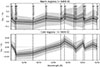 |
Fig. 11. Typical fit residual for some example absorption lines (indicated by dashed vertical lines). The light area marks the full range of residuals measured, the darker area the standard deviation and the solid line the mean. |
At this stage we have already verified the reproducibility of an average quiet Sun profile and excluded the groups of lines that show severe anomalous behavior. But even in the selected line list that resulted in a coherent atmosphere with physically expected values, we still cannot be completely certain about the atomic line parameters in use. However, since all fitted lines show too shallow and two deep line core-fits in different pixels and we find lines that show trends in either direction, we assume the residual uncertainties in the log(gf), excitation energy of the lower levels, and other line specific parameters to partly cancel out and hence play a minor role. Another potential reason are errors in the relative abundances, but since we found over and under estimated line cores of each dominant species in most spatial pixels, we also found this unlikely to be the main driver. It is nonetheless striking, that most lines show a clear and stable fit residual behavior relative to the other lines (see Figure 11). One generic reason that we could not rule out is that, with just three height nodes, the code cannot create the steep gradients required in the temperature and velocity stratification to account for the different formation heights of the lines. In the lowest atmospheric layers, steep temperature and velocity gradients are expected. However, these gradients are difficult to constrain with a few stronger absorption lines, since this information is encoded only in the near continuum line wings. When using many lines simultaneously each line forms at a different height and especially weaker lines provide information about the near-continuum region. A further indication for this are the remaining AWIVs in the topmost magnetic field map of the ML result. In our experiments, we found that seven nodes provided a well-constrained and reasonable temperature stratification. Unfortunately, due to the sensitivity and formation height of the observed lines, we were unable to constrain more nodes in the magnetic field and the Doppler velocity. However, as it currently stands, SPINOR does not permit a different number of nodes for different atmospheric parameters, making the compromise of three height nodes necessary.
Another generic reason might be the use of an LTE code. Lites & Athay (1972), Rutten (1988), Solanki & Steenbock (1988), and later also Shchukina & Trujillo Bueno (2001) have established that almost all neutral iron lines exhibit deviations from LTE. Asplund (2000) suggested that good fits to the observed lines could still be obtained by assuming LTE with an iron abundance of 7.46. Using lines with a wide range of atomic parameters can further help to minimize these effects from NLTE, because each transition will be influenced by the NLTE effects in different (and sometimes, opposing) ways. Indeed, Borrero & Bellot Rubio (2002) were able to fit multiple Fe lines to an average quiet Sun spectrum from an FTS atlas better than anticipated. Also Holzreuter & Solanki (2013) found that in such heavily temporally and spatially averaged line profiles NLTE effects are partially compensated. This agrees with our well reproduced average quiet Sun spectrum (see Figure 2). In our targeted observation we are presented with a spatially very highly resolved dataset from a single scan path, where the competition over atmospheric configuration between more LTE and more NLTE lines is no longer hidden in the average profile. Systematic departures of up to 5% (temperature) to 20% (velocities and magnetic field) for using LTE inversions in NLTE conditions on spatially resolved data were demonstrated by Smitha et al. (2020, 2021).
The aim of this study was the application of the many-line technique, as suggested by Riethmüller & Solanki (2019), to highly resolved observations. For comparability with their work, and since SPINOR was already successfully tested for many-line inversions, we used the same code here. We acknowledge that it is a LTE code and provides challenges in height node handling. Unfortunately, an exploration of both issues is outside the scope of the current work.
6.2. Noise
The undegraded spectra exhibit a relatively high noise level, which makes the deduced parameters less reliable (van Noort 2012). Especially in Q and U, the signal is almost buried in the 10−2 Ic noise, and for multiple lines outside the 5247 and 5250 regions it barely exceeds the noise floor.
In order to detect smale-scale features the scan speed cannot be arbitrary slow, as solar evolution would smear out the scene (See, Iglesias & Feller 2019, Figure 1). Therefore the number of frames accumulated per slit position cannot be higher. Further, deconvolution is needed to reach the diffraction limit and to resolve the desired small-scale features. Consequently, a certain increased noise level is inevitable for this type of diffraction limited observation.
In van Noort et al. (2025) we compared the noise and signal levels of FISS-SP with HINODE/SP. Since HINODE/SP observes two significant spectral lines over 112 spectral pixels while FISS-SP observes more than 150 spectral lines over 3840 spectral pixels we concluded that the total signal in our observations is considerably higher. For this study we used 85 lines distributed over 1281 spectral pixels. Considering the filtered deconvolution process applied, the S/N of FISS-SP is boosted further. Furthermore, van Noort & Doerr (2022) argued that data taken with a bigger aperture improves the signal content across the whole frequency domain for spatial resolution elements (See Section 3.3 in their paper). Because of the enhanced S/N in the restored data, the detection of true positive signals, especially from small-scale features, is improved (see Figure 8). Unfortunately, the higher absolute noise level of the deconvolved data remains problematic. For instance, in regions where there is no detectable signal the noise allows profiles to be fit with a relatively high background field (van Noort 2012; Danilovic et al. 2016). A prominent example of such an unrealistic high field was shown in Figure 5. Since the field strength is an unsigned quantity, the corresponding extracted maps may look relatively coherent. In such a case the best indication for noise-driven erratic behavior of the inferred field (as a vector) is given by the salt-and-pepper noise in the azimuth and inclination maps.
By combining the information from all 85 lines, weak information that might not exceed the noise level anywhere can be reliably detected (see Figure 9). Similar findings have been reported from stellar many-line approaches (Donati et al. 1997). Consequently, the extracted stratification gradients from many lines seem more realistic (see, Figure 5, Panels g–j). This agrees with the conclusion reached by Riethmüller & Solanki (2019) and suggests that, when many lines can be inverted simultaneously, the low spectral noise requirement of 10−3–10−5 can be relaxed. Also Díaz Baso et al. (2025) found a higher spectral sampling rate and undegraded data more beneficial than a lower noise level. The authors highlight that this effect is amplified when utilizing. multiple lines.
7. Conclusion
We used the spatially reconstructed dataset that was obtained with FISS-SP installed at the 1.6 m GST and deconvolved using the method from van Noort (2017). We applied the many-line inversion approach, proposed by Riethmüller & Solanki (2019), to this diffraction limited spectropolarimetric dataset. In line with their findings the results we obtained using manly-line approach are more robust against noise compared with a line-doublet inversion. The presented combination of spatial reconstruction and many-line inversion provides a way to mitigate losses from spatial degradation and shorter integration times, a conclusion recently also drawn by Díaz Baso et al. (2025). Thus, the approach discussed here effectively enables us to use spectropolarimetric data at the diffraction limit of large-aperture telescopes while maintaining the reliability of the inferred atmospheric configuration. Further, the combination of the information from many lines allows a signal that barely exceeds the noise floor to be reliably used. This effect relaxes the low noise requirement for precise polarimetry.
Our dataset included 171 relevant absorption lines that were reasonably well reproduced with an HSRA-based synthesis. It was therefore not expected that the inversion problem on spatially highly resolved data would not converge to a physically meaningful solution when incorporating all these lines. Instead we found that incorporating a line with anomalous behavior (e.g., because of poorly known atomic parameters) can lead to nonphysical results. Thus, a single bad line can potentially dominate the inversion outcome. In our tests we have seen that this can even drive an already converged solution to a nonphysical one and hence a better initial guess of the atmospheric configuration is not sufficient. These problems are not new and have been predicted already, for instance by Shchukina & Trujillo Bueno (2001), Borrero & Bellot Rubio (2002), Borrero et al. (2003), and Smitha et al. (2020, 2021). To avoid the inclusion of such lines with anomalous behavior we tested a selection strategy based on a statistical analysis of inversion results from individually inverted wavelength windows. In our case this resulted in the selection of 85 lines for the many-line inversion setup. Such an analysis provides a relatively cost-effective and fast method for identifying incompatible contributions from not well-understood lines.
While we had difficulties in extracting a coherent and physically meaningful model of the stratified solar atmosphere from two prominent lines, we showed that such issues can be alleviated by inverting many simultaneously observed spectral lines. Similar results are obtained if the atmospheres obtained individually from multiple simultaneously observed spectral windows are averaged. Here, the simultaneous inversion acts as a weighted average, using the knowledge of line response functions. Although the result of averaging inverted atmospheres obtained from a large group of spectral windows, each with a small number of lines, somewhat resembles that obtained fitting all of the lines simultaneously, the quality of the fitted spectrum is poorer for the latter. This is an indication that fit quality alone is not a decisive measure for the quality of the atmosphere deduced from the inversion process, the accuracy of the atomic parameters, (non-) LTE effects and the modeled complexity of the atmospheric stratification also have a significant influence. The adverse effect of using only a limited number of spectral lines on the spatial coherence of inversion results is at odds with the superior quality of the fit that is typically obtained in this way. As long as the ground truth is unknown, the coherence and physicality of the extracted atmosphere must serve as our proxies to determine the (relative) reliability of our results.
We have just begun to explore and analyze highly resolved solar many-line data. Stokes inversions depend on reliable and exact atomic data, including log(gf) values. Since the code can no longer so freely compensate for inaccuracies in the line parameters. The many-line technique presented here is pointing to a need for improved values for many lines in the solar spectrum. Further testing is required to determine if other regularization techniques and height node handling (as in SNAPI, see Milić & van Noort 2018), inversion codes that account for uncertainties in line parameters (as in globin, see Vukadinović et al. 2024), or NLTE-ready codes (e.g., SNAPI or NICOLE, see Socas-Navarro 2015) can mitigate these problems.
When the HINODE/SP data first arrived, the proposed Milne-Edington inversions provided many challenges (See for instance Orozco Suárez et al. 2007). Improvements of the available tools helped overcome these challenges (See for instance van Noort 2012). Since the decrease in fit quality we find when doing many-line inversions does not seem to be erratic, we expect that improvement in codes and atomic models will be needed to reach the fit quality that is currently available from few-line inversions. However, even though the presented approach does not improve the quality of the fits, using many lines represents a noticeable step forward in terms of coherence, stability, and sensitivity. Finally, it allows for a higher spatial resolution, since it is more robust against noise. Because of the availability of modern large format sensors, unlike Díaz Baso et al. (2025), we do not see a strong tension between wavelength range and spectral sampling, as long as data rates are not the limiting factor. For upcoming spectrographs we therefore strongly recommend to aim for a larger simultaneous spectral coverage to allow for such many-line inversions. The spectro-polarimeters SUSI (Feller et al. 2025) and SCIP (Katsukawa et al. 2025, submitted) on the Sunrise III observatory (Korpi-Lagg et al. 2025) are two further examples of instruments covering a broad wavelength range containing many spectral lines.
Acknowledgments
We appreciate the BBSO team for their efforts and contributions to the observation. We thank Tino Riethmüller for fruitful discussions in the early phase of this study. Finally, we would also like to thank the anonymous referee for the careful revision and helpful comments. The contribution of J. Hölken is supported by the International Max Planck Research School (IMPRS) for solar system science. The work of J. Chae and J. Kang was supported by the National Research Foundation of Korea (RS-2023-00208117, RS-2023-00273679). BBSO operation is supported by US NSF AGS-2309939 grant and New Jersey Institute of Technology (NJIT). GST operation is partly supported by the Korea Astronomy and Space Science Institute and the Seoul National University. This project has received funding from the European Research Council (ERC) under the European Union’s Horizon 2020 research and innovation programme (grant agreement No. 101097844–project WINSUN). This study is supported by US NSF grants AGS-2408174, 2401229, 2309939 and NASA grant 80NSSC24K1914. This research also benefited from the high-performance computing (HPC) capabilities at the Max Planck Institute for Solar System research (MPS) and the Gesellschaft für wissenschaftliche Datenverarbeitung mbH Göttingen (GWDG). The authors made a private donation to compensate for the CO2 emission created by the HPC usage. This work has made use of the VALD database, operated at Uppsala University, the Institute of Astronomy RAS in Moscow, and the University of Vienna. For the research we used NASA’s Astrophysics Data System (ADS).
References
- Allende Prieto, C., Ruiz Cobo, B., & Garcia Lopez, R. J. 1998, in Cool Stars, Stellar Systems, and the Sun, eds. R. A. Donahue, & J. A. Bookbinder, ASP Conf. Ser., 154, 813 [Google Scholar]
- Asplund, M. 2000, A&A, 359, 755 [NASA ADS] [Google Scholar]
- Asplund, M., Amarsi, A. M., & Grevesse, N. 2021, A&A, 653, A141 [NASA ADS] [CrossRef] [EDP Sciences] [Google Scholar]
- Balthasar, H. 1984, Sol. Phys., 93, 219 [NASA ADS] [CrossRef] [Google Scholar]
- Barnes, J. R. 2004, MNRAS, 348, 1295 [Google Scholar]
- Bigot, L., & Thévenin, F. 2006, MNRAS, 372, 609 [CrossRef] [Google Scholar]
- Borrero, J. M., & Bellot Rubio, L. R. 2002, A&A, 385, 1056 [NASA ADS] [CrossRef] [EDP Sciences] [Google Scholar]
- Borrero, J. M., Bellot Rubio, L. R., Barklem, P. S., & del Toro Iniesta, J. C. 2003, A&A, 404, 749 [NASA ADS] [CrossRef] [EDP Sciences] [Google Scholar]
- Brault, J. W. 1978, in Future Solar Optical Observations Needs and Constraints, ed. G. Godoli, 106, 33 [NASA ADS] [Google Scholar]
- Cao, W., Gorceix, N., Coulter, R., Coulter, A., & Goode, P. R. 2010, in Ground-Based and Airborne Telescopes III, eds. L. M. Stepp, R. Gilmozzi, & H. J. Hall, SPIE Conf. Ser., 7733, 773330 [Google Scholar]
- Castellanos Durán, J. S., Milanovic, N., Korpi-Lagg, A., et al. 2024, A&A, 687, A218 [NASA ADS] [CrossRef] [EDP Sciences] [Google Scholar]
- Chae, J., Park, H.-M., Ahn, K., et al. 2013, Sol. Phys., 288, 1 [NASA ADS] [CrossRef] [Google Scholar]
- Danilovic, S., van Noort, M., & Rempel, M. 2016, A&A, 593, A93 [NASA ADS] [CrossRef] [EDP Sciences] [Google Scholar]
- de la Cruz Rodríguez, J., Leenaarts, J., Danilovic, S., & Uitenbroek, H. 2019, A&A, 623, A74 [Google Scholar]
- del Toro Iniesta, J. C., & Ruiz Cobo, B. 2016, Liv. Rev. Sol. Phys., 13, 4 [Google Scholar]
- Díaz Baso, C. J., Milić, I., Rouppe van der Voort, L., & Schlichenmaier, R. 2025, A&A, 693, A272 [NASA ADS] [CrossRef] [EDP Sciences] [Google Scholar]
- Donati, J. F., Semel, M., Carter, B. D., Rees, D. E., & Collier Cameron, A. 1997, MNRAS, 291, 658 [Google Scholar]
- Feller, A., Gandorfer, A., Grauf, B., et al. 2025, Sol. Phys., 300, 65 [Google Scholar]
- Frutiger, C. 2000, Ph.D. Thesis, naturwissenschaften ETH Zürich, Nr. 13896 [Google Scholar]
- Frutiger, C., Solanki, S. K., Fligge, M., & Bruls, J. H. M. J. 2000, A&A, 358, 1109 [NASA ADS] [Google Scholar]
- Gingerich, O., Noyes, R. W., Kalkofen, W., & Cuny, Y. 1971, Sol. Phys., 18, 347 [Google Scholar]
- Goode, P. R., & Cao, W. 2012, in Ground-Based and Airborne Telescopes IV, eds. L. M. Stepp, R. Gilmozzi, & H. J. Hall, SPIE Conf. Ser., 8444, 844403 [Google Scholar]
- Goode, P. R., Coulter, R., Gorceix, N., Yurchyshyn, V., & Cao, W. 2010, Astron. Nachr., 331, 620 [NASA ADS] [CrossRef] [Google Scholar]
- Heiter, U., Lind, K., Bergemann, M., et al. 2021, A&A, 645, A106 [EDP Sciences] [Google Scholar]
- Hölken, J., Doerr, H.-P., Feller, A., & Iglesias, F. A. 2024, A&A, 687, A22 [NASA ADS] [CrossRef] [EDP Sciences] [Google Scholar]
- Holzreuter, R., & Solanki, S. K. 2012, A&A, 547, A46 [NASA ADS] [CrossRef] [EDP Sciences] [Google Scholar]
- Holzreuter, R., & Solanki, S. K. 2013, A&A, 558, A20 [NASA ADS] [CrossRef] [EDP Sciences] [Google Scholar]
- Holzreuter, R., & Solanki, S. K. 2015, A&A, 582, A101 [NASA ADS] [CrossRef] [EDP Sciences] [Google Scholar]
- Iglesias, F. A., & Feller, A. 2019, Opt. Eng., 58, 082417 [Google Scholar]
- Iglesias, F. A., Feller, A., Nagaraju, K., & Solanki, S. K. 2016, A&A, 590, A89 [NASA ADS] [CrossRef] [EDP Sciences] [Google Scholar]
- Katsukawa, Y., del Toro Iniesta, J. C., Solanki, S. K., et al. 2025, Sol. Phys., submitted [Google Scholar]
- Korpi-Lagg, A., Gandorfer, A., Solanki, S. K., et al. 2025, Sol. Phys., 300, 75 [Google Scholar]
- Kosugi, T., Matsuzaki, K., Sakao, T., et al. 2007, Sol. Phys., 243, 3 [Google Scholar]
- Kurucz, R. L. 2018, in Workshop on Astrophysical Opacities, ASP Conf. Ser., 515, 47 [NASA ADS] [Google Scholar]
- Kurucz, R. L., Hubeny, I., Stone, J. M., MacGregor, K., & Werner, K. 2009, AIP Conference Proceedings (AIP), 43 [Google Scholar]
- Laverick, M. 2019, Ph.D. Thesis, Faculty of Science, KU Leuven, Leuven, Belgium [Google Scholar]
- Lites, B. W., & Athay, R. G. 1972, BAAS, 4, 212 [Google Scholar]
- Lites, B. W., Elmore, D. F., & Streander, K. V. 2001, in Advanced Solar Polarimetry–Theory, Observation, and Instrumentation, ed. M. Sigwarth, ASP Conf. Ser., 236, 33 [Google Scholar]
- Milić, I., & van Noort, M. 2018, A&A, 617, A24 [Google Scholar]
- Neckel, H. 1999, Sol. Phys., 184, 421 [Google Scholar]
- Orozco Suárez, D., Bellot Rubio, L. R., Del Toro Iniesta, J. C., et al. 2007, PASJ, 59, S837 [CrossRef] [Google Scholar]
- Pakhomov, Y. V., Ryabchikova, T. A., & Piskunov, N. E. 2019, Astron. Rep., 63, 1010 [NASA ADS] [CrossRef] [Google Scholar]
- Riethmüller, T. L., & Solanki, S. K. 2019, A&A, 622, A36 [NASA ADS] [CrossRef] [EDP Sciences] [Google Scholar]
- Riethmüller, T. L., Solanki, S. K., & Lagg, A. 2008, ApJ, 678, L157 [Google Scholar]
- Ruiz Cobo, B., Quintero Noda, C., Gafeira, R., et al. 2022, A&A, 660, A37 [NASA ADS] [CrossRef] [EDP Sciences] [Google Scholar]
- Rutten, R. J. 1988, in IAU Colloquium 94: Physics of Formation of FE II Lines Outside LTE, eds. R. Viotti, A. Vittone, & M. Friedjung, Astrophys. Space Sci. Lib., 138, 185 [Google Scholar]
- Ryabchikova, T., Piskunov, N., Kurucz, R. L., et al. 2015, Phys. Scr., 90, 054005 [Google Scholar]
- Schüssler, M., & Vögler, A. 2006, ApJ, 641, L73 [Google Scholar]
- Shchukina, N., & Trujillo Bueno, J. 2001, ApJ, 550, 970 [NASA ADS] [CrossRef] [Google Scholar]
- Shenstone, A., & Blair, H. 1929, London Edinburgh Dublin Philos. Mag. J. Sci., 8, 765 [Google Scholar]
- Sinjan, J., Solanki, S. K., Hirzberger, J., Riethmüller, T. L., & Przybylski, D. 2024, A&A, 690, A341 [NASA ADS] [CrossRef] [EDP Sciences] [Google Scholar]
- Smitha, H. N., Holzreuter, R., van Noort, M., & Solanki, S. K. 2020, A&A, 633, A157 [NASA ADS] [CrossRef] [EDP Sciences] [Google Scholar]
- Smitha, H. N., Holzreuter, R., van Noort, M., & Solanki, S. K. 2021, A&A, 647, A46 [NASA ADS] [CrossRef] [EDP Sciences] [Google Scholar]
- Socas-Navarro, H. 2015, Astrophysics Source Code Library [record ascl:1508.002] [Google Scholar]
- Solanki, S. K., & Steenbock, W. 1988, A&A, 189, 243 [NASA ADS] [Google Scholar]
- Solanki, S. K., & Stenflo, J. O. 1984, A&A, 140, 185 [NASA ADS] [Google Scholar]
- Solanki, S. K., & Stenflo, J. O. 1985, A&A, 148, 123 [NASA ADS] [Google Scholar]
- Stenflo, J. O. 1973, Sol. Phys., 32, 41 [NASA ADS] [CrossRef] [Google Scholar]
- Sütterlin, P., Schröter, E. H., & Muglach, K. 1996, Sol. Phys., 164, 311 [CrossRef] [Google Scholar]
- Tsuneta, S., Ichimoto, K., Katsukawa, Y., et al. 2008, Sol. Phys., 249, 167 [Google Scholar]
- van Noort, M. 2012, A&A, 548, A5 [NASA ADS] [CrossRef] [EDP Sciences] [Google Scholar]
- van Noort, M. 2017, A&A, 608, A76 [NASA ADS] [CrossRef] [EDP Sciences] [Google Scholar]
- van Noort, M., & Doerr, H. P. 2022, A&A, 668, A151 [NASA ADS] [CrossRef] [EDP Sciences] [Google Scholar]
- van Noort, M., Lagg, A., Tiwari, S. K., & Solanki, S. K. 2013, A&A, 557, A24 [NASA ADS] [CrossRef] [EDP Sciences] [Google Scholar]
- van Noort, M., Hölken, J., Doerr, H.-P., et al. 2025, A&A, 704, A215 [NASA ADS] [CrossRef] [EDP Sciences] [Google Scholar]
- Vukadinović, D., Smitha, H. N., Korpi-Lagg, A., et al. 2024, A&A, 686, A262 [NASA ADS] [CrossRef] [EDP Sciences] [Google Scholar]
Appendix A: Atomic data listings
Atomic line data used for the many-line SPINOR inversion sorted by central wavelength (CWL) and separated in spectral regions.
Same as A.1 but for lines that were disregarded during the selection process.
All Tables
Atomic line data used for the many-line SPINOR inversion sorted by central wavelength (CWL) and separated in spectral regions.
All Figures
|
Fig. 1. Continuum image of the observed active region extracted from the restored scan. The scan direction is from top to bottom along the y-axis, the axis labels are in arcseconds, the intensity is normalized to I/IC. The blue box indicates the ROI used for this study; the black arrow indicates the direction to the disk center. |
| In the text | |
|
Fig. 2. Comparison of the computed spectrum using the HSRA model with a normalized Stokes I profile from an averaged FISS-SP flat-field measurement. We allowed the code to adjust for microturbulence and temperature offset. The bar above the profile indicates the spectral windows R01–R18 from Table 2. |
| In the text | |
|
Fig. 3. Comparison of atmospheric parameters deduced from the 18 selected spectral windows (see Table 2), separated by type of solar feature. The main columns show properties of granules, inter-granular lanes, bright points, umbra, and umbral dots. Each column is sub-divided by dashed lines into the values of the parameters at the different optical depth nodes. Each row refers to one atmospheric parameter (temperature, LOS velocities, and field strength). Each spectral window is represented by a symbol, indicating the mean value of the retrieved parameter from all pixels corresponding to the given physical parameter, and a range bar, indicating the standard deviation. The excluded windows are marked with an ×-symbol. The gray entry indicates the mean of the finally used 14 spectral windows and the black entry the result from the simultaneous many-line inversion (see main text for a detailed discussion). |
| In the text | |
|
Fig. 4. Zoomed-in image of the lower left panel of Figure 3 (see legend in that figure) showing the field strength statistics for granular pixels. The threshold of (≈650 G) is highlighted with a dotted horizontal line. |
| In the text | |
|
Fig. 5. Typical fit and stratification for the blended region R01 including ten spectral lines for a selected granulation pixel. Panels (a–d): Observation, and synthetic profiles in Stokes I, V, Q, and U in relative values of I. The R01 profile corresponds to the inversion result from the individual inversion of this region, while the ML profile was synthesized using the atmospheric configuration extracted from the many-line inversion result (see Section 5). Panels (e–f): Continuum image (e) of the granule with the selected pixel marked by the orange plus sign (+) and the corresponding map of the magnetic field strength (f) in the log(τ) = 0 node. Panels (g–j): Derived stratification for temperature (g), vLOS (h), turbulence (i) and field strength (j). The values at the log(τ ) nodes are indicated with a symbol, the line represents the spline fit. Orange is the stratification for the selected pixel from the inversion result, green shows the mean and range of the values from the green box indicated in the middle panel, and red shows the stratification for the many-line atmosphere of the selected pixel. |
| In the text | |
|
Fig. 6. Maps of the temperature, LOS velocities, and magnetic field strength at log(τ) ∈ {0.0, −0.8, −2.0}; and height independent inclination, azimuth, and χ2. This result is inferred with the traditional approach using the Fe I doublet that consists of the 5247.05 Å and the 5250.20 Å lines. We have used four cycles of 75 iterations each, the axis tick marks are in arcseconds (see main text for a discussion). In all figures negative vLOS denotes a flow toward the observer (i.e., up-flow) and positive LOS velocities denote a flow away from the observer (i.e., down-flow). |
| In the text | |
|
Fig. 7. Same as Figure 6, but for the final many-line setup using two cycles a 75 iterations and 85 lines. |
| In the text | |
|
Fig. 8. Side-by-side comparison of magnetic field strength maps from both setups in four example areas. The continuum images in the middle panel correspond to the adjacent field maps panel. All tick marks are in arcseconds and within the reference frame of Figures 6 and 7 and are marked with white boxes therein. |
| In the text | |
|
Fig. 9. Typical example of the observed and fitted profiles for both setups. The topmost panel shows Stokes I/IC while the other panels show relative signal strength of V, Q, and U respectively. IC corresponds to average quiet Sun continuum intensity. |
| In the text | |
|
Fig. 10. Zoom in for Figure 9 on the two iron lines fitted in the traditional approach. Please refer there for legend. On this scale the difference in the fit quality, especially in I and Q becomes visible. We contribute the obvious discrepancy of both fits with Stokes U to residual, field depended, cross-talk from Stokes I in the data. |
| In the text | |
|
Fig. 11. Typical fit residual for some example absorption lines (indicated by dashed vertical lines). The light area marks the full range of residuals measured, the darker area the standard deviation and the solid line the mean. |
| In the text | |
Current usage metrics show cumulative count of Article Views (full-text article views including HTML views, PDF and ePub downloads, according to the available data) and Abstracts Views on Vision4Press platform.
Data correspond to usage on the plateform after 2015. The current usage metrics is available 48-96 hours after online publication and is updated daily on week days.
Initial download of the metrics may take a while.