| Issue |
A&A
Volume 705, January 2026
|
|
|---|---|---|
| Article Number | A17 | |
| Number of page(s) | 19 | |
| Section | Astronomical instrumentation | |
| DOI | https://doi.org/10.1051/0004-6361/202557378 | |
| Published online | 07 January 2026 | |
A new broad K/Ka-band receiver (18.0–32.3 GHz) for the Yebes Observatory’s 40 meter radio telescope★
1
Centro de Desarrollos Tecnológicos, Observatorio de Yebes (IGN),
19141
Yebes, Guadalajara,
Spain
2
Observatorio Astronómico Nacional (OAN, IGN),
Calle Alfonso XII, 3,
28014
Madrid,
Spain
3
Departamento de Astrofísica Molecular, Instituto de Física Fundamental (IFF-CSIC),
Calle Serrano 121,
28006
Madrid,
Spain
★★ Corresponding authors: This email address is being protected from spambots. You need JavaScript enabled to view it.
; This email address is being protected from spambots. You need JavaScript enabled to view it.
; This email address is being protected from spambots. You need JavaScript enabled to view it.
Received:
23
September
2025
Accepted:
19
November
2025
Abstract
Since 2010, the 40 m radio telescope of the Yebes Observatory has been devoted to very long baseline interferometry (VLBI) and single-dish observations. Up until 2019, it covered frequency bands between 2 GHz and 90 GHz in discontinuous and narrow radio windows that met the needs of the European VLBI Network (EVN) and the Global Millimeter VLBI Array (GMVA). The situation changed in 2019 when new receivers were built and installed at the telescope for the Q- (31.5–50 GHz) and W- (72–90.5 GHz) bands in the frame of the Nanocosmos1 project, a synergy project funded by the European Research Council. The 18.5 GHz instantaneous bandwidth is now fully covered in the two polarisations with 16 fast Fourier transform (FFT) spectrometers of 38 kHz resolution. This has allowed us to achieve an unprecedented level of ultra-sensitivity for line surveys, leading to the discovery of around 95 molecules in space over the last six years. These results have encouraged the construction of a new low-noise cryogenic receiver between 18 GHz and 32.3 GHz for the 40 m radio telescope with orthogonal polarisations (H & V) and 19 kHz of spectral resolution. Due to the frequency resolution requirement and the limited number of FFT boards, the band has been split into two sub-bands for each polarisation: low-band (18–26 GHz) and high-band (26–32.3 GHz), with eight FFT spectrometers of 1 GHz instantaneous bandwidths per sub-band and per polarisation. Alternatively, the receiver can be configured to analyze the full receiver band (18–32.3 GHz) in a single polarisation (either H-pol or V-pol). Here, we present the characteristics of the receiver and the first astrophysical results demonstrating its performance. A detailed analysis of the radio frequency interferences (RFIs) generated by satellite down-link communications and its impact on spectroscopic studies of the interstellar and circumstellar media is also provided. In this context, we conclude that the radio astronomy community must continue to strive to protect the still RFI-free K/Ka radio windows from harmful radiocommunication signals.
Key words: line: identification / instrumentation: detectors / techniques: spectroscopic / telescopes / circumstellar matter / ISM: molecules
Based on commissioning observations carried out with the Yebes 40 m telescope which is operated by the Spanish National Geographic Institute (IGN, Ministerio de Transportes y Movilidad Sostenible).
© The Authors 2026
 Open Access article, published by EDP Sciences, under the terms of the Creative Commons Attribution License (https://creativecommons.org/licenses/by/4.0), which permits unrestricted use, distribution, and reproduction in any medium, provided the original work is properly cited.
This article is published in open access under the Subscribe to Open model. This email address is being protected from spambots. You need JavaScript enabled to view it. to support open access publication.
1 Introduction
The 40 m radio telescope of the Yebes Observatory was observing in the K band (21–25 GHz) and Q band (41–49 GHz) since 2010 and 2013, respectively, with a reduced instantaneous bandwidth of 500 MHz and dual-circular polarisations (see e.g. Agúndez et al. 2015a). In 2016, the intermediate frequency (IF) bandwidths of both receivers were increased to 2.5 GHz (de Vicente et al. 2016; Gómez-Garrido et al. 2020). Since 2010, observations in the W band have also been possible with a receiver using a superconductor-isolator-superconductor (SIS) mixer and an instantaneous bandwidth of 600 MHz, mainly for very large baseline interferometry (VLBI) observations (see e.g. Issaoun et al. 2019).
In 2019, two new broadband receivers were built for the Q (31.5–50 GHz) and W (72–90.5 GHz) bands in the framework of the Nanocosmos1 project. They were installed at the Yebes 40 m radio telescope, replacing the previous Q- and W-band receivers and providing an instantaneous bandwidth of 18.5 GHz in each band and in both linear polarisations. A detailed description of the 40 m radio telescope, the broadband Nanocosmos receivers, the fast Fourier transform (FFT) spectrometer back-ends, and the telescope and receivers performance is provided in Tercero et al. (2021). From this time to 2024, the available K-band receiver at the 40 m radio telescope was connected to an available narrow-band FFT back-end to cover a limited bandwidth of 500 MHz between 21 GHz and 25 GHz.
The Nanocosmos Q-band receiver has been used to provide a large number of new detections of interstellar molecules in the last six years, mostly within the QUIJOTE2 project, an ultra-sensitive line survey of TMC-1 (Cernicharo et al. 2021a, 2024a). Line surveys are the best tool for exploring the chemical composition of interstellar and circumstellar clouds. In this context, the QUIJOTE line survey has led to the detection of more than 70 molecules in this cold pre-stellar dark core. Some of them are very polar species with relatively low abundances, such as the 17 S-bearing species discovered in TMC-1 (Cernicharo et al. 2021b, 2024b; Agúndez et al. 2025, and references therein), radicals H2C3N, H2C4N, and HCCCHCN (Cabezas et al. 2021, 2023, 2025), double cyanide derivatives of methane (NCCH2CN) and ethylene (NCCHCHCN; Agúndez et al. 2024), or the protonated species of very abundant molecules such as HCCS+ (Cabezas et al. 2022a), HCCS+ (Cernicharo et al. 2021c), and NC4NH+, among others (Agúndez et al. 2023a), (Agúndez et al. 2023b, and references therein).
One of the most significant results of QUIJOTE is the discovery, through the standard method of line by line detection, of low-dipole but very abundant pure hydrocarbons such as CH2CHCCH (Cernicharo et al. 2021d), c-C6H4 (Cernicharo et al. 2021a), CH2CCHCCH (Cernicharo et al. 2021e), c-C5H6, and c-C9H8 (Cernicharo et al. 2021f), as well as the radical H2CCCH (Aqúndez et al. 2021; Agúndez et al. 2022), long carbon chain CH2CCHC4H (Fuentetaja et al. 2022), and c-C5H4CCH2 (Cernicharo et al. 2022). These neutrals, together with some cations such as l-C3H3+ (Silva et al. 2023), certainly play an important role in the growth of larger hydrocarbons and polycyclic aromatic hydrocarbons (PAHs) in TMC-1 (Cernicharo et al. 2022).
Indene (c-C9H8) is the only PAH discovered directly from its rotational spectrum (Cernicharo et al. 2021f). However, cyano derivatives of benzene and naphthalene have previously been reported in TMC-1 using stacking techniques with the GOTHAM line survey (see also Cernicharo et al. (2021g, 2024a); McGuire et al. (2018, 2021)). Moreover, recently, the 1- and 5-cyano derivatives of acenaphthylene have been reported in TMC-1 with the QUIJOTE line survey (Cernicharo et al. 2024a) and cyano derivatives of pyrene and coronene have been also claimed by the GOTHAM3 team through the statistical stacking approach (Wenzel et al. 2024, 2025a,b).
Motivated by the success of the QUIJOTE line survey, a new broadband low-noise cryogenic receiver covering the 18–32.3 GHz range named ASTROREC, has been developed at the Yebes Observatory. Its main goal is continuing the discovery of new complex molecules and larger PAHs by the traditional, robust, and solid method of line-by-line detection.
This paper is devoted to the presentation of the new ASTROREC K/Ka-band receiver installed at the 40 m radio telescope of the Yebes Observatory (Sect. 2). Detailed information on the receiver components are given in Sects. 2.1–2.6. The performance of the receiver, the telescope efficiencies in the K/Ka-band, and the problems in the astronomical data caused by radio frequency interferences (RFIs) are described in Sect. 3. The first astronomical results are given in Sect. 4.
2 The receiver
The new ASTROREC K/Ka-band receiver has been installed at the Yebes 40 m radio telescope, retaining the optics in front of the feed described in Tercero et al. (2021). The astronomical specifications were based on a single-pixel receiver with dual linear polarisation (H & V) and a maximum receiver noise temperature of 20 K across the 18–32.3 GHz range. The 18 GHz lower frequency limit was selected to accommodate the reception of interesting molecular lines at 18.2 GHz (e.g. HCCCN at 18 196 MHz) and the upper frequency limit was set to overlap with the Q-band Nanocosmos receiver (31.5–50 GHz), providing the 40 m radio telescope with a full frequency coverage from 18 GHz to 50 GHz. The upper band of ASTROREC might occasionally allow for the reception of Deep Space Network (DSN) down-link signals (27–32.3 GHz).
Additionally, the ASTROREC frequency range imposes the use of customised waveguide sizes for some front-end devices, namely, the orthomode transducer (OMT), directional couplers, and low noise amplifiers (LNAs), because there is no standard waveguide covering the full specified range. A customised rectangular waveguide 9.2 × 4.6 mm with a 16.245 GHz cut-off frequency for the fundamental mode was selected.
The receiver can be used for dual-circular polarisation detection in a 4 GHz bandwidth centered at 22 GHz by placing a quarter-wave plate (QWP) in front of the dewar’s window to convert linear to circular polarisation for VLBI observations. Two calibration devices for VLBI observations are included in the system: a noise diode for amplitude calibration that can be switched ON/OFF at an 80 Hz rate and a frequency comb generator that provides 10 MHz-spaced frequency tones for phase calibration. Amplitude calibration for single-dish observations is achieved using the same hot-cold system of the Q-band and W-band receivers (see Tercero et al. 2021 and Sect. 3.4).
Figure 1 shows the block diagram of the whole receiving system. The different parts of the receiver (the front end, down-conversion units, and spectrometers) are described in the following sub-sections.
2.1 The cooled front end
The tertiary optics of this K/Ka-band receiver basically consist of an elliptical mirror that creates a frequency-independent image of the sub-reflector at the feed position with a beam radius of 38 mm. A view of the assembled cooled front end set-up can be seen in Fig. 2.
The receiver feed consists of a corrugated horn with a planohyperbolic dielectric lens for phase correction at its aperture. The horn is made of aluminum and the lens is made of PTFE4. The whole lensed horn has been optimised in terms of impedance matching and predicted aperture efficiency on the 40 m radio telescope using the CST Studio Suite5 and GRASP6 software. The aperture diameter of the corrugated horn is 160 mm, and the length is 270 mm. The measured reflection coefficient is better than −20 dB in the specified frequency range and the predicted illumination efficiency, based on the measured radiation patterns from the feed, ranges between 75% in the lower part of the band and 62% in the higher part. The measured directivity of the feed alone is about 29 dBi at mid-frequency (i.e. 25 GHz). The corrugated horn has a circular waveguide output of 5.6-mm radius, although a circular-to-square waveguide transition has been included in the setup to fit the 9.2-mm-side square waveguide of the OMT. This waveguide transition is included in the measurements described above.
Due to the OMT configuration, the front end naturally provides dual-linear polarisation for the whole band of interest. However, the system allows us to use a dielectric QWP placed in front of the cryostat window at ambient temperature to provide dual circular polarisation between 20–24 GHz, which is the frequency range of interest for VLBI. The implemented QWP is based on a grooved plate made of HDPE7. Assuming that the loss tangent of this material is 1 × 10⁻³, the estimated losses of the QWP are about 0.04 dB.
The OMT is connected at the output of the feed horn, and provides two orthogonal linear polarisation components for the whole band of interest (García et al. 2022). The input port interface is a 9.2-mm-side square waveguide, and the two outputs are 9.2 × 4.6 mm rectangular waveguides. The OMT topology is the so-called double-ridge OMT (Reyes et al. 2012), which provides adequate trade-off between ease of manufacturing and bandwidth for this application. It can be easily manufactured from two pieces based on a ’split-block’ construction, where the two halves are joined together. In this case, the OMT is made of aluminum and it has been electromagnetically simulated and optimised using CST Studio Suite. The reflection coefficients measured at the two output ports are better than −17.7 dB and −19.0 dB in the ASTROREC frequency range limits, and the average insertion losses are about 0.04 dB and 0.03 dB for each H and V polarisation path, respectively.
The front end also includes one 30 dB directional coupler per polarisation to inject an amplitude and a phase calibration signal. Both couplers have been made following a multihole waveguide configuration. The coupled path is a parallel waveguide terminated with two coaxial K-connector (2.92 mm) transitions: one for signal injection and the other matched with a 50 Ω load. The measured reflection coefficient is lower than −32 dB, whereas the insertion losses are lower than 0.25 dB. The coupling coefficient is 24 ± 1.5 dB.
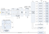 |
Fig. 1 Block diagram of the ASTROREC 18–32.3 GHz receiving system. |
2.2 The cryostat
The cryostat uses a two-stage Gifford-McMahon cryocooling system, model RDK-408S from SHI Cryogenics8. The outer dimensions of the cylindrical dewar are 583 mm in length and 370 mm in diameter.
Inside the dewar, there is another cylinder attached to the intermediate stage at 30 K and covered with multilayer isolation (MLI), which serves as a radiation shield between the cold stage (at 10 K) and the dewar. The dewar plate in front of the feed horn has a 200-mm-diameter hole, covered with a corrugated PTFE window that allows for the incoming radiation to pass through while maintaining the necessary vacuum inside the dewar. The opposite plate (cryostat hot stage) provides the interfaces for the coaxial RF outputs and calibration signal inputs, connections to the room-temperature electronics, LNA biasing lines, vacuum sensor, and vacuum pump ports.
Within the cryostat (see Fig. 2), the base of the feed horn is directly attached to the cold stage plate. A pair of flexible copper thermal straps connect the LNAs to the cold plate to reduce the physical temperature of the active devices. The operating temperatures are about 30 K and 10 K at the intermediate and cold stages, respectively. Two additional temperature sensors have been placed on one of the LNAs and on the feed, next to its aperture, providing typical values of 13 K and 58 K, respectively. To minimise the thermal conduction between the cryogenic components and the outer interface, ultra-low thermally conductive semi-rigid coaxial cables were used for the RF output and calibration signals (model UT-085B-SS). The intermediate and cold stages are joined with three G10 glass fiber structures to improve stability.
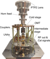 |
Fig. 2 Internal view of the cryostat showing the cooled front-end components. |
2.3 The low noise amplifiers
The cryogenic 18–32.5 GHz LNAs used in the receiver front end (see Fig. 3) are based on a hybrid (discrete components) design developed at Yebes Observatory. Each amplifier incorporates three stages of 0.1 × 50 μm discrete InP high electron mobility transistor (HEMT) devices produced by Diramics9. The first stage device is based on an experimental material with a lower gate Schottky barrier that is optimised for lower cryogenic noise temperature and power dissipation, while the others are made of standard material (López-Fernández et al. 2024).
The internal matching networks were produced in-house by laser milling on a DUROIDTM 6002 microwave substrate 0.127 mm thick. The boxes were machined in brass and gold plated with soft gold. The input interface is implemented with a waveguide for a low-loss connection to the horn. There is no standard waveguide covering the required 18–32.3 GHz band and a customised rectangular waveguide 9.2 × 4.6 mm with a 16.245 GHz cut-off frequency for the fundamental mode was used. The output is a standard coaxial 2.92 mm connector for easy coaxial cable routing in the cryostat.
Each LNA stage was individually biased. The bias point was optimised for a good compromise between noise, reflection, gain, and flatness. Noise and gain were measured at 7 K physical temperature using a custom non-standard waveguide size cryogenic variable-temperature load developed to match the input waveguide of the amplifier. The physical temperature of the load was varied between 20 K and 50 K under a proportional integral derivative (PID) control to perform the noise power measurement. The error in the measured noise temperature is ±0.4 K, dominated by the precision of the temperature sensor diodes. Additional details of the construction and measurements can be found in Diez-Gonzalez et al. (2024).
Noise and gain plots of the amplifiers measured in the laboratory at 7 K are shown in Fig. 4 together with the total noise temperature of the complete receiver at 13 K as measured with the instrumentation in the laboratory, not with the FFT spectrometers. It should be mentioned that the ripple in the receiver noise temperature is due to standing waves associated with the hot and cold loads used for the Y-factor measurements and, hence, a rather flat behavior is expected for the actual receiver temperature across the receiver frequency range.
The main results of the measurements of the standalone amplifiers are summarised in Table 1. In addition to the commonly reported noise temperature and gain, data of the complete set of noise parameters of the amplifier at cryogenic temperature in terms of noise waves referred to the input of the amplifier and to the impedance of the waveguide using the nomenclature proposed by Meys (1978) were also obtained (see Fig. 5) following the procedure described in Amils et al. (2024). This data is rarely provided due to the difficulty of its measurement, but offers valuable insight on the performance, allowing for an easy estimation of the possible degradation of the receiver sensitivity as a function of input mismatch.
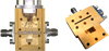 |
Fig. 3 Left: complete LNA without cover and coaxial input and output connectors. Right: final configuration with input waveguide. The overall block dimensions are 43 × 38 × 11 mm, including the waveguide transition. |
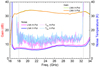 |
Fig. 4 Gain and noise temperature of the cryogenic LNA measured at 7 K physical temperature compared with the total noise of the complete receiver cooled at 13 K. The ripple shown in receiver noise is due to standing waves associated with the hot and cold loads used for the Y-factor measurements. |
Typical measured results of the cryogenic LNA across the 18–32.5 GHz range.
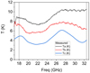 |
Fig. 5 Noise parameters of the cryogenic LNA expressed following Meys’ noise wave representation, based on two waves at the LNA input. Ta represents the non-correlated part of the wave going into the amplifier (it is the noise temperature measured using a matched load at the source). Tb represents the non-correlated part of the noise wave emitted from the LNA towards the source. Finally, Tc represents the modulus of the noise waves correlation (see Meys 1978). |
2.4 Room-temperature RF chain and down-conversion units
Immediately after the cryostat, two short low-loss coaxial cables transport the signals (H & V) to a pre-amplifier module. Each pre-amplifier channel is composed of an isolator, an amplifier, and a band-pass filter between 18 GHz and 32.3 GHz for the image rejection prior to the first down-conversion. The pre-amplifier module increases the level of the cryostat output signals by 20 dB. It also isolates the noise contributions from the next receiver stages.
Next, the first down-converter shifts the RF range (18–32.3 GHz) to the first IF range (1–15.3 GHz). This conversion is performed using a local oscillator (LO) at 17 GHz, which is 1-Hz tunable in the range of 15.5–17.5 GHz and allows for the Doppler effect to be corrected in spectral line observations. In addition, equalisers are included in each channel to flatten the power spectrum of the H and V signals across such a broad band.
The first IF signals are transported from the receiver room down to the back-end room via RF-over-fiber optic links (RFoF), where a band splitter module divides the IFs in two sub-bands for each polarisation: low (1–9 GHz, 8 GHz of bandwidth) and high (9–15.3 GHz, 6.3 GHz of bandwidth). The high sub-band is then mixed with a 18 GHz phase-locked oscillator (PLO). This analog signal conditioning is required to accommodate the signals to the inputs of the baseband down-converters that operate in the range of 1–9 GHz. Table 2 provides the frequency values and ranges for the frequency down-conversion in the receiver.
A matrix switch and eight-way power splitters select and distribute the 16 (8 sub-bands × 2 polarisations) signals to the bank of baseband down-converters, whose outputs are connected to 16 FFT spectrometer boards.
Each of the eight baseband dual-channel down-converters receives the signals (H & V) in the input range of 1–9 GHz. Afterwards, a slice of 1 GHz is filtered and down-converted with a fixed-frequency PLO to the DC − 1 GHz range to fit the input bandwidth requirement of the FFT spectrometer boards and to avoid aliasing during digital signal processing. These down-converters are equipped with variable attenuators to control the input power level to each FFT spectrometer board. The attenuation required for each of the 16 FFT boards is optimised using the hot load of the calibration system to ensure operations in the linear regime.
Table 3 shows the sky frequencies assigned to each down-converter and to each FFT spectrometer for both low and high sub-bands when the first LO is set at 17 GHz. Moreover, the auxiliary outputs of down-converter number 5 are used for VLBI observations, as they are routed to the VLBI digital baseband converter (DBBC) back-ends.
2.5 Spectrometers
The spectrum of the signals is computed with 16 FFT spectrometer digital boards arranged in two crates with 8 FFT boards each one. Their field programmable gate arrays (FPGAs) are loaded with a firmware that provides 65 536 channels along a bandwidth of 1 GHz, resulting in an equivalent noise band width (ENBW) of 19 kHz per channel.
As mentioned above, when observing the high band (26–32.3 GHz), the spectra provided by the FFT spectrometers must be reversed by software, due to the frequency conversion of the first IF with the PLO at 18 GHz in the band splitter module. Due to the image rejection filters in the pre-amplifier module, the spectra provided by the FFT spectrometers from 32.3 GHz to 34 GHz are useless. Nevertheless, this frequency range is already covered with the 40 m Q-band Nanocosmos receiver (31.5–50 GHz). The full set-up of band splitter, signal distributor, baseband down-converters, and spectrometers is shown in Fig. 6.
2.6 Calibration modules for VLBI
The amplitude and phase calibration system consists of two sub-systems, the RF module (with NoiseCal and PhaseCal), along with the power supply and control module. The RF module generates a frequency comb of 10 MHz-spaced tones from 18 GHz to 32.3 GHz, covering the whole RF receiver bandwidth, and an additive white Gaussian noise signal (AWGN) that can be switched ON/OFF at 80 Hz rate.
The tones are combined with the AWGN signal and injected in front of the LNAs, via the 30 dB directional couplers, as described in Sect. 2.1. The power supply and control module manage the operational status and power requirements of the RF components, providing essential dynamic control and monitoring functions for reliable system performance.
To achieve a good phase calibration performance, it is essential to maintain a stable and constant temperature within the RF module. This is done by using a Peltier cell together with the appropriate controller, a fan, and a radiator to dissipate the heat extracted by the Peltier cell.
The RF module is housed in a hermetically sealed metal case, insulated with foam to prevent thermal contact between the outside and the metal plate in which the RF components are integrated, thus maintaining a stable temperature of 20°C ± 0.1°C for ambient temperature changes in the range of 19°C−31°C.
Frequency values and ranges for the frequency down-conversion of the 18–32.3 GHz receiver.
Downconverter IF and sky frequencies.
3 Receiver performance
3.1 RFI monitoring
The electromagnetic spectrum is an asset that is regulated by different bodies: International Telecommunications Union (ITU) at a global scale, Conférence Européenne des Administrations des Postes et des Télécommunications (CEPT) at European level and, in the case of Spain, Secretary of State for Telecommunications and Digital Infrastructure (SETSI).
There are many terrestrial and satellite radio services (geostationary satellites, non-geostationary satellites in low Earth orbit, fixed and mobile services, radiolocation, radio-links, etc.) that emit in the frequency range of the ASTROREC receiver. As the radio astronomy service (RAS) is fully passive, it can use the whole band for observations, but it is only protected against interference in its allocated bands as primary or secondary service or where it has some protection under Article 5 of the ITU Radio Regulations (RR). These bands are summarised in Table 4.
In recent years, there has been a significant increase in allocated frequency bands and in the number of satellites in orbit due to the advent of mega-constellations. As a result, the ASTROREC receiver has to coexist with several signals from those radio services. Monitoring campaigns have been carried out to assess the radio environment in the ASTROREC frequency range at Yebes Observatory.
Observations were conducted on December 2 and 10, 2024, using low-frequency (18–26 GHz) and high-frequency (26–32 GHz) configurations, both with H & V polarisations. To monitor potential RFI sources that could affect astronomical observations, 30-second recordings were made at 5° azimuth intervals from 0° to 360° and at two elevation angles (5° and 45°).
The most significant RFI sources in terms of signal strength and spatial occurrence were automotive radar transmissions in the range 24.15–24.25 GHz, which show significant variations in day-to-night observations and some directivity related to surrounding roads and cities, geostationary satellite transponder signals, which produce strong effects in the 18–18.2 and 18.8–20.2 GHz ranges (see Fig. 7) and VSAT satellite communications. Importantly, no interference was observed within the primary RAS protected bands (see Table 4).
These results indicate that observations with the ASTROREC receiver should avoid sky regions near the geostationary arc. Given the complexity of astronomical scheduling, new software should be developed to implement geostationary satellite avoidance algorithms, analogous to existing sun avoidance protocols in telescope control systems. Our experience in sensitive astronomical observations (see Sect. 4) indicates that even at several degrees from Clark’s belt, some RFI contamination is detected at different frequency ranges below 20.2 GHz. Unfortunately, the 24.15–24.25 GHz range is already compromised for astronomical purposes. For some sources, depending on its position in the sky and observing time, RFI becomes a real concern across the entire K/Ka band.
Moreover, despite the excellent rejection of the mixers and filters, traces of the RFI signals arise in the image band during high sensitivity observations due to the large amplitude of these RFIs. The image signals from the 24.15–24.25 GHz radars will eventually appear in the 28–27 GHz band, while signals from satellites operating at 20.0–20.2 GHz would also be detected at 31–32 GHz. In addition, very narrow and strong spurious signals are detected through the receiver band, originating from the different LOs in the system. Fortunately, these spurious signals are easily identified and removed during data reduction, especially when two different settings of the LOs are used during the observations.
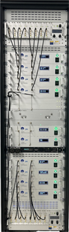 |
Fig. 6 Integrated cabinet with fiber optic receivers, band splitter, signal distributor, baseband down-converters, and spectrometer crates. |
Allocated bands for radio astronomy in the frequency range of ASTROREC receiver.
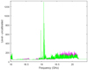 |
Fig. 7 Geostationary satellite transponder signals measured at Az = 165°, El = 45°. Purple and green spectrum correspond to H and V polarisations, respectively. |
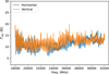 |
Fig. 8 Measured receiver noise temperature of the complete ASTROREC system installed at the 40 m radio telescope using a hot and a cold load in front the dewar’s window and the FFTS back-ends. |
3.2 Receiver noise temperature
The receiver noise temperature (Trec) takes into account the contribution from all elements located between the calibration system and the final detectors (i.e. feed, OMTs, waveguides, amplifiers, down-converters, and FFT back-ends) to the total noise of the spectrum. This measurement allows us to check the performance of the complete system and it is required to calibrate the astronomical data (see Sect.3.4). Then, Trec can be calculated using loads at different temperatures through the well-known Y-factor method, whose equations are the following (see e.g. Kramer 1997),
![Mathematical equation: $\[T_{\mathrm{rec}}=\frac{T_{\mathrm{hot}}-Y T_{\mathrm{cold}}}{Y-1}, Y=\frac{V_{\mathrm{hot}}}{V_{\mathrm{cold}}},\]$](/articles/aa/full_html/2026/01/aa57378-25/aa57378-25-eq1.png) (1)
(1)
where Vhot and Vcold are the back-end counts when a hot and a cold load is presented at the dewar’s input window, respectively, while Thot and Tcold are the physical temperatures of the hot and cold loads, respectively.
For the characterisation of the receiver, two loads (hot and cold) based on microwave absorber foams were manually placed just in front of the dewar’s window. These absorbers were large enough to cover the physical dimensions of the window and to avoid reflections with other elements of the receiver cabin. For the hot load, the absorber was at room temperature (295 K) while for the cold load, the absorber was immersed in liquid nitrogen to cool it down to 77.3 K.
Detected counts using the FFT back-ends described in Sect. 2.5 were registered for H and V polarisations in both low and high configurations (see Sect. 2.4). As shown in Fig. 8, the measured Trec values are typically below 15 K for all receiver frequencies, indicating a very good performance of the entire chain from the receiver feed to the FFT back-ends. The ripple in the traces are caused by standing waves between the dewar’s window and the loads used for the measurements.
3.3 Stability
The performance of a radio telescope is limited by the noise and gain stability of its receivers. The most common method for detecting weak signals involves long-time integrations, which requires a stable receiver behavior. The stability measurement addresses possible gain fluctuations of the receiver and mechanical coupling with elements in the receiver chain due to vibrations.
Gain fluctuations of the order of 10−4 per second or less provide flat enough baselines for the astronomical data. Figures A.1 and A.2 show the normalised back-end counts of each FFT backend section of the ASTROREC receiver when observing a hot load for a total time of ~30 minutes in February 2025, in the low and high configurations of the receiver, respectively. Typical relative peak-to-peak values for the fast variation fluctuations of about 5 × 10⁻⁴ per second are measured. Slower drifts over 20–30 min are mainly due to temperature variations, but they do not significantly affect astronomical data because these are usually collected using shorter integration times. The system was found to be sufficiently stable for astronomical observations that involve position, wobbler, or frequency switching individual observations that are 5–10 min long (see Sect.4).
3.4 Data calibration and cold load noise temperature
Due to the versatile optical design of the 40 m antenna, the automatic hot-cold load calibration system used for the Q- and W-band Nanocosmos receivers is also usable for ASTROREC data calibration. In such a system, the hot load is a low reflectivity microwave absorber at ambient temperature; whereas the cold load is another absorber cooled down to a physical temperature of about 17 K inside a small cryostat (see Tercero et al. 2021). Remarkably, the pointing and focusing models of the Q-band receiver are used (and are perfectly suited) for the ASTROREC receiver, demonstrating the optimal performance of the optical system.
The system temperature (Tsys), which gives the noise performance temperature of the receiver (Trec, see Sect. 3.2) plus the atmosphere temperature (Tsky), which can be derived from
![Mathematical equation: $\[T_{\mathrm{sys}}=V_{\mathrm{sky}} \frac{T_{\mathrm{hot}}-T_{\mathrm{cold}}}{V_{\mathrm{hot}}-V_{\mathrm{cold}}},\]$](/articles/aa/full_html/2026/01/aa57378-25/aa57378-25-eq2.png) (2)
(2)
where Vhot, Vcold, Thot, and Tcold are those defined in Eq. (1), while Vsky is the back-end count pointing to the sky.
However, as the physical size of the mirror intercepting the beam towards the cold load cryostat was optimised for frequencies above 30 GHz, the equivalent noise temperature of the cold load (Tcold) between 18 GHz and 30 GHz could significantly diverge from its physical temperature due to the truncation of the beam. Therefore, to provide an accurate calibration for the ASTROREC data, an effective value for Tcold across the band needs to be obtained. For this purpose, a set of measurements using the Nanocosmos calibration system were performed to characterise the equivalent noise temperature of the cryogenic cold load. The raw Trec obtained when assuming that the effective noise temperature of the cold load is constant and equal to its physical temperature (i.e. ~17 K) is represented in the top plot of Fig. 9. Compared to the actual noise temperature in Fig. 8, we can observe an apparent noise increase due to the truncation effects, which is more noticeable at lower frequencies, as expected. From this result, it is possible to derive the effective value of Tcold that allows us to recover the actual value of Trec measured in optimal conditions. This effective Tcold value is represented in the bottom plot of Fig. 9 and listed in Table 5. The measured Trec obtained when using the effective Tcold values is represented in the middle plot of Fig. 9. In conclusion, applying this correction it is possible to reliably utilise the automatic calibration system, despite its optical limitations for the current frequency range.
The complete calibration procedures and the single-dish observing modes are the same as those described in Tercero et al. (2021) for the Q- and W-band Nanocosmos receivers. These procedures include atmospheric attenuation corrections using the ATM code (Cernicharo 1985; Pardo et al. 2001).
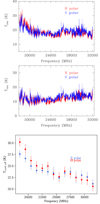 |
Fig. 9 Top: measured receiver noise temperature (uncorrected) of the ASTROREC system using the Nanocosmos calibration system and assuming Tcold=17 K. Middle: measured receiver noise temperature of the ASTROREC system using the Nanocosmos calibration system and corrected using the effective noise temperature of the cold load. Bottom: calculated effective noise temperature of the cryogenic cold load of the Nanocosmos calibration system (see Sect. 3.4). |
Equivalent noise temperature of the cold load.
3.5 Forward efficiency
The forward efficiency (ηF) can be obtained from skydip observations, where the sky emissivity is measured at different air masses (i.e. different elevations). Then, ηF and τ, the zenith opacity of the atmosphere, are fitted according to the following equation,
![Mathematical equation: $\[T_{\mathrm{sys}}=T_{\mathrm{rec}}+T_{\mathrm{sky}}=T_{\mathrm{rec}}+T_{\mathrm{atm}} \eta_{\mathrm{F}}\left(1-e^{-\tau A}\right)+\left(1-\eta_{\mathrm{F}}\right) T_{\mathrm{amb}},\]$](/articles/aa/full_html/2026/01/aa57378-25/aa57378-25-eq3.png) (3)
(3)
where Tatm is the effective temperature of the atmosphere at Yebes Observatory, estimated using the ATM code (Cernicharo 1985; Pardo et al. 2001) and local weather conditions, while A is the air mass and Tamb is the ambient temperature.
Observations were performed on April 30, 2025, in the early morning with clear skies. Several measurements were taken, with the antenna moving from 5 to 85 degrees in elevation, corresponding to airmasses of 11.5 to 1.0, respectively. During these skydip drifts, the total power measured for each FFT spectrometer was averaged and stored every 100 ms. Two different receiver configurations were used to cover the entire K/Ka frequency range: the lower part of the band (18–26 GHz) and the higher one (26–32 GHz). Afterwards, the ηF values were obtained for each FFT section and polarisation.
Figure 10 shows the fit for a frequency of 25.5 GHz, in the middle of the band, corresponding to the last section of the FFT in the low band configuration of the receiver. The results are summarised in Table 6, where the averaged values of both polarisations are shown for each central frequency of the sub-band.
3.6 Aperture, main beam efficiencies, and Jy/K conversion
The aperture efficiency of the radio telescope (ηA) has been theoretically estimated at three different frequencies in the observing frequency range, resulting in values of 0.72 at 18 GHz, 0.65 at 25 GHz and 0.57 at 32.3 GHz (see Table 7). This efficiency has been calculated as the product of the illumination efficiency (ηi), the efficiency of the mirrors (ηm1 for the main reflector, ηm2 for the sub-reflector, and ηmn for the other mirrors), the losses introduced by the membrane at the vertex (ηmbr) and the ohmic losses (ηohm) of the structure. The illumination efficiency, which has been simulated using GRASP software, amounts to 0.75 at 18 GHz, 0.68 at 25 GHz and 0.62 at 32.3 GHz. On the other hand, the efficiencies of the mirrors have been calculated using Ruze’s formula (Ruze 1966) for each wavelength (λ), assuming root-mean-square (RMS) surface errors (σ) of 175 μm for the main reflector, 50 μm for the sub-reflector, and 25 μm for the rest of the mirrors along the ray path (see Eq. (4) and Tercero et al. 2021), expressed as
![Mathematical equation: $\[\eta_{\text {mirror }}=e^{-\left(\frac{4 \pi \sigma}{\lambda}\right)^2}\]$](/articles/aa/full_html/2026/01/aa57378-25/aa57378-25-eq4.png) (4)
(4)
The losses introduced by the membrane are based on laboratory measurements of the dielectric material (García-Pérez et al. 2017). Finally, the ohmic losses are considered to be negligible at these frequencies.
The aperture efficiency can also be measured from continuum observations of point-like sources with calibrated fluxes. We derived ηA across the full bandwidth of the ASTROREC receiver using pointing drifts towards Saturn on April 17, 2025, following the same method described in Tercero et al. (2021). These pointing drifts were performed using all FFTS back-end boards simultaneously, each one operating as a total power detector. Therefore, all channels of a complete 1.0 GHz-width FFT board are averaged at every stored azimuth and elevation position during the drifts.
The apparent size of the planet (~15.9″) and its flux at the central frequency of each FFT section were obtained from ASTRO (part of GILDAS software10) for the time and date of the observation. At this date, Saturn reached its maximum elevation at ~45°, enabling the measurement of ηA as a function of elevation between 15° and 45°. We note that no significant variations of ηA were found with respect to elevation or for the two polarisations. The resulting aperture efficiencies for each frequency were obtained from the mean value at all measured elevations in H and V polarisations and are summarised in table 6. We note a slightly lower (about a 7%) efficiency value at 31.5 GHz measured with the ASTROREC K/Ka-band receiver compared to the value observed at 32 GHz with the Nanocosmos Q-band receiver (see Tercero et al. 2021). This could result from a better matching of the optical system to the Q-band frequencies but also from the expected 10% calibration error in the observations.
From the obtained ηA values, the Jy/K conversion factors are derived for punctual sources given in Table 6. There is a discrepancy between the measured aperture efficiency (Table 6) and the estimated one (Table 7) of about a 15%. Assuming this discrepancy is entirely due to the RMS surface error of the main reflector, we obtained the ηm1 value 0.77 at 32.3 GHz. Using Eq. (4), we can estimate the RMS surface error of the primary reflector associated with these efficiencies, which results in a value of σ = 378 μm. This result is consistent with the RMS surface error of the main reflector obtained by fitting the error beams over a full Moon observation (see Sect. 3.7 and Tercero et al. 2021). However, at the lower end of the band (i.e 18 GHz), a RMS surface error of ~400 μm cannot explain the discrepancy between the estimated and measured efficiency by itself.
Therefore, other effects such as defocusing, astigmatism, or calibration errors may also contribute to a decrease in the measured aperture efficiency. The hypothesis of astigmatism is supported by the last surface accuracy measurements performed in June 2019 with the help of the prime focus microwave holography system (see López-Pérez et al. (2012) and López-Pérez et al. (2014) for details on the 40 m radio telescope holography system). These surface measurements are shown in Fig. 11. In the plot on the left, the resulting surface accuracy was 225 μm RMS. However, some degree of astigmatism can be observed. If an aberration term for astigmatism is subtracted through leastsquares fitting, then the resulting surface accuracy is 184 μm RMS (see the plot on the right of Fig. 11). Therefore, the astigmatism term adds 130 μm RMS of surface error. The fitted astigmatism has an amplitude of 0.7 mm at the edge of the reflector. It has been verified with microwave holography that the amplitude of the astigmatism changes with temperature, from day to night, and it is larger in summer than in winter.
The main beam efficiency (ηMB) is the fraction of power received which enters through the main beam. It is usually derived from continuum observations of planets whose angular diameter fills the main beam. However, due to the large values of the half power beam widths (HPBW) of the telescope at the frequencies of the ASTROREC receiver, no planet in the sky has an apparent size large enough to fill the main beam. Nevertheless, this value can be derived from ηA as these two efficiencies are related via the antenna illumination (see Kramer 1997; Tercero et al. 2021). Using this relation we obtained the ηMB values shown in Table 6.
HPBW, efficiencies, and Jy/K conversion of Yebes 40 m radio telescope along the K/Ka band.
Theoretically estimated contributions to the aperture efficiency of the antenna (ηA).
 |
Fig. 11 40 m radio telescope surface measured with microwave holography (scale in microns), before astigmatism fitting (left plot, 225 μm RMS) and after astigmatism fitting (right plot, 184 μm RMS, 0.7 mm astigmatism amplitude). |
3.7 Moon coupling and beam pattern
To evaluate the percentage of power lost through the secondary and error beams of the radio telescope, we quantified the coupling between the Moon and the beam pattern (ηMoon). Most of the astronomical sources are rather compact and their sizes in the sky are well below ~0.5° (the apparent size of the Moon on the sky), meaning that this efficiency is a useful measurement for interstellar clouds with sizes similar to that of the Moon.
We performed pointing drifts at different frequencies towards the full moon on 13 February 2025 in the K/Ka band. The spatial resolution of the scans was ~23″. We used all FFTS sections, each of them operating as a continuum detector. Figure 12 shows selected pointing drifts in the K/Ka band. From Krotikov & Pelyushenko (1987) we estimate a Moon brightness temperature of ~270 K at 11 mm which has to be compared to the antenna temperature of 225 K obtained from the observations. This gives ηMoon (K band) = 0.83 ± 0.10.
The beam pattern can be described by the main beam and different error beams produced by secondary lobes (i.e. misalignments in the optical path) and the large-scale deformations at the primary reflector such as astigmatism, panel frame misalignments, and panel deformations. The total power scans towards the Moon at 14.6, 11.8, and 10.5 mm were used to derive the beam pattern of the Yebes 40 m radio telescope down to approximately −30 dB (see Fig. 13), following the procedure described in Tercero et al. (2021). We derived independent parameters of the beam pattern for azimuth and elevation drifts. The estimated beam parameters for the averaged results of azimuth and elevation scans are summarised in Table 8.
The relative normalised percentage of the power of the main beam (see Table 8) over a source of 30″ varies between 87% at 14.6 mm and 83% at 10.5 mm. In our fits, the first secondary lobe contributes less than 2% of the power at all frequencies and we did not include it in Table 8. Large-scale deformations (first error beam), small errors of individual panels (second error beam), and panel frame misalignments (third error beam) contribute to power losses of ~13–17%, increasing with frequency.
The correlation length of the deformations and RMS of the surface errors associated with each error beam can be obtained according to the procedure described in Greve et al. (1998) (see also Tercero et al. (2021)). Figure 14 shows the fits from which correlation lengths and RMS surface errors are obtained. We obtain deformation correlation lengths of 6.0, 3.8, and 1.03 m for the first (large-scale deformations), second (panel frame misalignments) and third (panel deformations) error beam, respectively. These values agree with the expected length of these inhomogeneities and the values derived in Tercero et al. (2021) for data at 7 mm and 3 mm.
The associated RMS values of the surface errors are 250 μm (1st error beam), 215 μm (2nd error beam), and 175 μm (3rd error beam) which gives a combined (root-sum-square, RSS) value of 373 μm which matches the RMS surface errors estimated for the Yebes 40 m radio telescope by Tercero et al. (2021).
It must be mentioned that this overall RSS value is not directly comparable with the surface accuracy provided by microwave holography measurement given in the previous section because holography subtracts the pointing errors and axial and lateral defocusing terms, while the moon coupling data include all the factors impacting on aperture efficiency. In addition, the computed RMS surface error associated with the third error beam, which corresponds to panel deformations, is 175 μm, whereas the surface panels were reported to have less than 75 μm RMS, according to their surface error budget (including gravity, wind, and thermal deformations). The actual value for the surface error of each panel was verified as being lower than the specification (65 μm RMS on average) with the help of photogrammetry measurements on every surface panel provided by the manufacturer.
In conclusion, there seems to be a combination of large-scale deformations (such as defocussing or astigmatism) or calibration errors that are impacting the final aperture efficiency of the radio telescope. This requires further investigation, starting with the thermal gradient analysis of the radio telescope from the data of the recently installed thermal sensor network. For this purpose, 165 PT100 thermal sensors (4-wire, class 1/10) were installed in the radio telescope structure in specific locations defined after a finite element method (FEM) analysis. Once data from at least one year are available, the influence of temperature on the structure of the radio telescope will be determined, along with its effects on efficiency, mirror alignment, and deformations of the main reflector, as well as pointing accuracy and variations in focal distance. The measured thermal behavior will make it possible to define and install a thermal control system to mitigate those effects, with the ultimate goal of creating a model that allows for corrections to be applied during observations.
 |
Fig. 12 Selected pointing drifts in the K/Ka band. Azimuth and elevations drift are depicted in black and red, respectively. |
 |
Fig. 13 Composite profiles observed around the full moon (black points) together with the synthetic best-fit profiles (red curves). |
Beam parameters of Yebes 40 m radio telescope.
 |
Fig. 14 Best-fit values (solid circles) of the widths (top panel) and amplitudes (bottom panel) of the error beams. Dashed lines fit these values in order to obtain the correlation length (L) and the RMS value of the surface errors (σ). |
4 Astronomical results and performances
4.1 First VLBI observations
On November 1st, 2024 the Yebes 40 m radio telescope took part in an EVN (European VLBI Network) Network Monitoring Experiment (N 24 K 3), and first interferometric fringes were observed towards J1801+4404 in baselines between the Yebes 40 m (Ys) and the Sardinia 64 m (Sr), the Urumqi 25 m (Ur), Onsala 20 m (On) and both KASI 21 m antennas at PyeongChang (KC) and at Yonsei (Ky). Fringes were obtained in eight contiguous 32 MHz wide channels between 22107.49 MHz and 22361.49 MHz in both left and right circular polarisations with similar amplitudes across the bands. The circular polarisation was obtained by installing a quarter-wave plate in front of the receiver cryostat window, as described in Sect. 2.1. Strong signal-to-noise ratios of around 100 for Ys-Sr and 10 for Ys-Ky in a 4 s integration time scan were obtained. The intensity of cross polarisation was approximately between 15% and 20%. System noise temperature (Tsys) and system equivalent flux density (SEFD) values were impacted by poor weather during the observation, with values 120 K and 600 Jy respectively. Under good weather conditions, these values usually improve to 80 K and 430 Jy. Figure 15 shows the auto-correlation and cross-correlation plots for the Yebes-Sardinia baseline (Ys-Sr), for scan 22 on source J2203+3145. Detailed results can be seen in JIVE services website11.
 |
Fig. 15 Auto-correlation and cross-correlation plots for scan 22 on source J2203+3145 that show the Yebes band-pass for every frequency channel, affected by the DBBC2 digital back-end response, and the amplitude and phase of the Yebes–Sardinia correlation showing a low level of cross-polarisation or leakage (cyan and blue curves). |
4.2 Single-dish observations
TMC-1 (αJ2000= 4h41m41.9s and δJ2000 = +25°41′27.0″) has been extensively observed with the Yebes 40 m radio telescope in the frame of the QUIJOTE line survey (Cernicharo et al. 2021a, 2024a). In addition to TMC-1, ultra-sensitive observations of IRC+10216 (αJ2000 = 9h47m57.36s and δJ2000= +13°16′44.4″) have also been performed with the same telescope in the Q band (Pardo et al. 2022).
TMC-1 and IRC+10216 have been the reference sources for the commissioning of the new K/Ka-band receiver. The observing time in the 18–26 GHz range towards TMC-1 is 226 hours, while in the 26–32 GHz range it is only of 80 hours. The selected observing procedure was frequency switching with a throw of 11.7 MHz which minimises the larger frequency standing waves. Observations were carried out between August 2024 and March 2025. In order to avoid potential ghost lines produced in the down-conversion chain, the LO setting was changed four and five times in the 18–26 GHz and 26–32 GHz frequency ranges, respectively. Figure 16 shows the resulting spectrum in the whole band of the receiver.
Figure 17 shows the observed spectrum towards IRC+10216. Observing time between 18 GHz and 26 GHz is 12 hours, and 10 hours for data above 26 GHz. Observations were achieved in wobbler switching using the new wobbling secondary mirror installed at the telescope (Albo et al., in prep.). The 17.8–26.3 GHz frequency range was previously observed towards IRC+10216 with the 100 m Effelsberg radio telescope by Gong et al. (2015). Taking into account that the emission of cyanopolyynes and CnH radicals in IRC+10216 arises from a ring of ~15″ of radius (Agúndez et al. 2015b), and the different telescope beam efficiencies and source dilution in the beam, we found a very good agreement between the intensity of the observed lines in Fig. 17 and those of Gong et al. (2015).
4.3 RFI effects on astronomical signals
As noted in Sect. 3.1, the 18–20.2 GHz range is heavily affected by RFI. We also found that the intensity and frequency of the spurious RFI signals are strongly dependent on the position of the telescope relative to the satellites orbiting in the geostationary Clarke’s belt. These effects are common to all observatories and have previously been reported at National Radio Astronomy Observatory (NRAO)12.
During the time covered by our observations, we found that the 18.3–18.8 GHz range in TMC-1 and IRC+10216 is relatively free of RFI. However, the 18.8–20.2 GHz one is practically useless in TMC-1, while the 19.3–20.2 GHz range is free of RFI in IRC+10216. In L183 all data below 23 GHz were found to be useless in the observing period too. The frequencies affected by RFI are clearly visible in Figures 16 and 17. They are indicated by the thick horizontal red lines. Taking into account that for IRC+10216 the wobbling throw was of 240″, we conclude that RFI signals change over very small angular scales. This evidence suggests that the detection of RFI signals may vary depending on the specific time of day, with radio astronomy observations being most adversely affected between noon and late afternoon.
In spite of these RFI spurious signals, strong astronomical lines are clearly detected in the 18.0–18.2 GHz and 18.8–20.2 GHz ranges. As an example, we show in Fig. 18 the J = 1–0 transition of SiS at 18.154 GHz with its clear blue maser emission peak at vLSR = −40 km s−1 (see e.g. Henkel et al. 1983; Fonfría et al. 2006; Gong et al. 2017; Fonfría et al. 2018); the RFI at the frequency of this line is severe (see Fig. 17) and translates into a noisy background with systematic spectral features that avoid that noise decreases with the square root of the integration time. At the frequencies of the SiS J = 1–0 line, the expected theoretical noise is around 0.4 mK. However, it is measured to be ~7 mK limiting clear 4σ detections to lines with intensities ≥28 mK. Moreover, the baseline introduced by the RFI reduces the calibration accuracy for lines below the 28 mK level. In the case of low intensity emission only narrow features can be explored in the RFI zones. Weak broadband features in these frequency zones are fully submerged in the RFI spectral pattern.
A second zone of fully unreliable data is the 24.15–24.25 GHz range, which is unfortunately heavily contaminated by vehicle radar emitters (see Sect. 3.1). Other narrow ranges of RFI are indicated in Figures 16 and 17. The RFI frequency ranges could slightly change from source to source due to the Doppler shift introduced by the velocity corrections of each source.
In the frequency ranges affected by RFI the astronomical spectra measured in H and V polarisations show practically the same spectral features. However, the RFI intensity in H and V depends on the parallactic angle of the telescope with respect the RFI source which can be strongly polarised.
The results presented here clearly indicate the effect of RFI on real observations: no spectral search for molecules without well-known frequencies can be performed in the RFI zones. Spectral statistical stacking of data affected by RFI is strongly not recommended in view of the level of contamination appearing at high sensitivity in these zones. The useful data that can be obtained for a given source depend on the observatory scheduling time along the year. For TMC-1 the loss in frequency coverage is ~2 GHz, namely, 14% of the receiver band when the observations are scheduled between summer and winter at the Yebes 40 m radio telescope.
 |
Fig. 16 Observed spectrum of TMC-1 in the frequency range 18.0–32.3 GHz using the new K/Ka-band receiver of the 40 m radio telescope of the Yebes Observatory. The data have been gathered in frequency switching. The negative features produced after folding have not been flagged in this figure. The ordinate is the antenna temperature corrected for atmospheric and telescope losses in milli-Kelvin. The different panels show always the same data but with different intensity scales. The abscissa is the rest frequency adopting a local standard of rest velocity (vLSR) of 5.83 km s−1 (Cernicharo et al. 2020a). Observing time in the 18–26 GHz range is 226 hours, while above 26 GHz is only 80 hours. RFI zones are indicated by the red lines in the bottom panel. They correspond to the frequency ranges 18.00–18.30, 18.80–20.25, 22.05–22.15, 23.00–23.10, and 24.15–24.25 GHz. In spite of the strong interferences at these frequencies, intense astronomical lines are easily detected as it can be seen in the different panels. |
 |
Fig. 17 Observed spectrum of IRC+10216 between 18.0 GHz and 32.3 GHz using the new K/Ka-band receiver of the Yebes Observatory. The data have been gathered in wobbler switching and are shown without any baseline subtraction. A box car smoothing of six channels has been applied. The ordinate is the antenna temperature corrected for atmospheric and telescope losses in milli-Kelvin. The different panels show the same data but with different intensity scale. The abscissa is the rest frequency; i.e. it was frequency-corrected for a vLS R velocity of −26.5 kms−1 (Cernicharo et al. 2000). Observing time between 18 GHz and 26 GHz is 12 hours and it is 10 hours for data above 26 GHz. Frequency ranges with severe RFI for IRC+10216 are 18.00–18.30, 18.80–19.30, 22.05–22.15, 23.01–23.06, and 24.12–24.25 GHz. They are indicated by red horizontal lines. Despite the intense interferences in these frequency ranges, strong astronomical lines are easily detected. |
 |
Fig. 18 Observed line of SiS J = 1–0 towards IRC+10216. The abscissa in the bottom axis is rest frequency in MHz adopting a local standard of rest velocity of −26.5 km s−1 (Cernicharo et al. 2000). The upper abscissa axis represents the local standard of rest velocity adopting a frequency for the 1–0 line of SiS of 18154.8861 MHz. The ordinate is the antenna temperature in milli-Kelvin. The line is in the middle of a heavy RFI frequency zone. As a consequence, the measured noise is 7 mK while its expected value should be 0.4 mK. Moreover, this extra noise does not look like a white noise but appears with spectral structures arising from the RFI signals. |
4.4 Ammonia in TMC-1
In TMC-1, no water maser emission was detected, but we can confirm that no RFI is present in this protected frequency zone. Several inversion lines of NH3 and 15NH3 that are also within a protected frequency range have been observed. No RFI has been found for any of these lines in TMC-1, L183, and IRC+10216. The ammonia lines towards TMC-1 are shown in Fig. 19. One of the largest improvements provided by broadband line surveys is that we observe all lines of a given molecule falling in the receiver band at once. Hence, all of them will have common systematic effects on the pointing and calibration of the lines. This permits us to perform reliable models for the line intensities and cloud properties.
To our knowledge, it is the first time that the transitions 15NH3 (1,1) and the NH3(3,3), together with the hyperfine components of the NH3 (2,2) line, are reported in TMC-1. Since the first detection of ammonia in space (Cheung et al. 1968), this molecule has been considered as a thermometer of the kinetic temperature of the gas (Cheung et al. 1969a,b; Morris et al. 1973; Walsmley & Ungerechts 1983). Although the analysis of the observed ammonia lines is beyond the scope of this work, a preliminary study could take advantage of the high S/N achieved in our observations. The (1,1) transition is clearly affected by line opacity, while the (2,2) is more optically thin.
We used the collisional rates between o/p-NH3 and p-H2 calculated by Loreau et al. (2023) to compute the expected emission of ammonia in TMC-1. We adopted a kinetic temperature of 9 K (Agúndez et al. 2023a) and a volume density of 2 × 104 cm−3. Line opacities can be, in principle, derived from an analysis of the hyperfine components of the (1,1) transition using the GILDAS software. However, the observed lines profile require at least two layer cloud components to explain qualitatively the (1,1) and (2,2) intensities. The densest component has n(H2) = 2 × 104 cm−3, and total column densities for ortho and para ammonia (A and E spin states) of N(p-NH3) = N(o-NH3) = 1.2 × 1014 cm−2. The adopted abundance ratio p-NH3/p-15NH3 is 570. The second layer component has also a kinetic temperature of 9 K, a density of 1000 cm−3 and a column density of 6 × 1012 cm−2. It affects mainly the (1,1) line with negligible effect on the (2,2) line and on the (1,1) one of 15NH3. For the (1,1) spectrum in the top panel of Fig. 19 the red dashed line corresponds to the one layer component model. The thin red line in all panels of this figure corresponds to the two layer cloud components. In addition to the two layer cloud structure we also need two velocity components (5.83 km s−1 and 6.50 km s−1) to reproduce the line profiles of all observed transitions. Finally, the (3,3) line cannot be reproduced with the same kinetic temperature as it involves high energy levels. Its intensity is extremely sensitive to the adopted kinetic temperature. Nevertheless, only a small change in TK from 9 K to 11.5 K allows us to reproduce the observed intensity of this inversion line of ammonia rather well (see the thick red line). Hence, our observations of ammonia point to a kinetic temperature profile much more complex than the single kinetic temperature adopted for TMC-1.
 |
Fig. 19 Observed inversion lines of NH3 and 15NH3. The species and the quantum numbers are indicated at the top of each panel. None of these lines is affected by RFI. The abscissa is the rest frequency in MHz adopting a vLS R of 5.83 km s−1 (Cernicharo et al. 2020a). The ordinate is the antenna temperature in milli-Kelvin. For the (2,2) inversion line the green scale corresponds to the intensity in milli-Kelvin but with a zoom of a factor 10 for the data and the synthetic model. The red line corresponds to the computed theoretical spectrum described in the text. Two velocity components have been considered for all ammonia lines (5.8 km s−1 and 6.5 km s−1). |
Observed lines of HC7NH+ in TMC-1.
4.5 Improved rotational constants for HC7NH+
Another example of the advantage of the new sensitive broadband observations in the K/Ka band is the detection of all transitions within the receiver band of HC7NH+ (transitions from J = 17–16 up to J = 28–27), a molecule previously discovered with the QUIJOTE line survey by Cabezas et al. (2022b). In order to derive more accurate molecular constants for this species a new set of observed frequencies was obtained by fitting a Gaussian line profile to the observed data. A window of ± 2 MHz was selected around the expected frequency of each transition. A vLS R of 5.83 km s−1 was adopted for TMC-1 (Cernicharo et al. 2020a). The derived frequencies and line intensities are given in Table 9, while the observed lines in the K/Ka band are shown in Fig. 20. The line parameters reported by Cabezas et al. (2022b) were obtained during the first observing runs of the QUIJOTE line survey. We have remeasured these frequencies using the last data of the survey (Cernicharo et al. 2024a). The new frequencies in the Q band are also given in Table 9. All lines from J = 17–16 up to J = 40–39 can be fitted with the standard Hamiltonian for a linear molecule providing B = 553.939017 ± 0.000046 MHz and D = 3.736 ± 0.023 Hz. The standard deviation of the fit is 5.8 kHz. A significant improvement in the uncertainty of the rotational and distortion constants has been achieved. The red lines in Fig. 20 correspond to the synthetic line profiles derived using the cloud parameters used for this molecule in the Q band by Cabezas et al. (2022b). Only the source diameter has been changed from 80″ to 90″ to fill the larger beam width of the telescope in the K/Ka band (see Sect. 3.5). The agreement between the model and the observations is excellent.
The transitions of other protonated species such as HC3O+ (Cernicharo et al. 2020b), CH3CO+ (Cernicharo et al. 2021h), HC3S+ (Cernicharo et al. 2021c), HCCS+ (Cabezas et al. 2022a), or the anion C5N− (Cernicharo et al. 2008, 2020c), which have strong emission lines in the QUIJOTE line survey are also easily observed in the present K/Ka-band data. A detailed analysis of these data and additional results in TMC-1 and IRC+10216 will be presented in forthcoming papers.
 |
Fig. 20 Observed lines of HC7NH+ towards TMC-1 in the K/Ka band. The abscissa is the LSR velocity in km s−1. The ordinate is the antenna temperature in millikelvin. The red line is the computed theoretical spectrum using the column density and rotational temperature derived by Cabezas et al. (2022b) and adopting a source diameter of 90″. The two spectra marked in green as RFI correspond to frequencies severely affected by RFI. Note the broad spectral features due to RFI present in the J = 18–17 line. |
5 Summary and conclusions
This paper presents the development, implementation, and commissioning of ASTROREC, a new broad K/Ka-band cryogenic receiver (18.0–32.3 GHz) for the Yebes Observatory 40 m radio telescope. The receiver significantly enhances the telescope’s capabilities by providing a wide instantaneous bandwidth, dual orthogonal polarisations (H & V), and spectral resolution of 19 DDkHz. Circular polarisation observations are also feasible with the help of a dielectric QWP placed in front of the cryostat window. Designed to complement existing Nanocosmos Q- and W-band receivers, ASTROREC fills a relevant observational gap, enabling continuous coverage from 18 GHz to 50 GHz and supporting both VLBI and single-dish astronomical observations.
Comprehensive laboratory and on-site performance evaluations have been introduced. They confirm the receiver’s low noise temperature (typically below 15 K across most of the band) and stable gain characteristics, ensuring high-sensitivity observations over long integration times. Calibration with the hot and cold load system of the Q- and W-band receivers was used and refined to account for frequency-dependent effects, including the computation of the equivalent cold load noise temperature for ASTROREC.
In addition, forward and aperture efficiencies were measured using skydip and planetary observations. The results demonstrate good performance with forward efficiencies around 0.95 and aperture efficiencies ranging between 0.58 and 0.46, depending on frequency. An important point in this regard is the discrepancy between the aperture efficiency derived from astronomical measurements and that measured with microwave holography. While holography-based surface accuracy measurements indicate an RMS of approximately 225 μm, astronomical observations suggest a higher effective surface error of around 378 μm. This difference may arise from additional large-scale deformations such as astigmatism, defocusing effects, or calibration uncertainties; thus it would require further analysis.
Initial astronomical observations, including VLBI fringes and single-dish spectral line surveys of TMC-1 and IRC+10216, validate the scientific potential of the receiver. Despite the challenges posed by RFI from satellite communications and car radars, particularly below 20.2 GHz and around 24.15–24.25 GHz, mitigation strategies such as adaptive scheduling and LO reconfigurations can be effective in minimising the effects of RFI.
Future works will be focussed on further improving RFI mitigation techniques. In addition, thermal gradient analysis from the data provided by the recently installed network of thermal sensors is planned to understand the discrepancies related to the aperture efficiency of the radio telescope. In conclusion, the ASTROREC receiver makes the 40 m radio telescope an even more powerful tool for advancing astrochemical studies, including the detection of complex and heavy molecules and PAHs in interstellar and circumstellar environments.
Acknowledgements
We thank the Spanish Ministry of Science and Innovation (MCIN/AEI/ 10.13039/501100011033) and “ERDF A way of making Europe” for funding support through projects PID2019-107115GB-C21, PID2019-107115GBC22, PID2022-137980NB-I00, and PID2023-147545NBI00. A. Vidal-García acknowledges support from the Spanish grant PID2022-138560NB-I00, funded by MCIN/AEI/10.13039/501100011033/FEDER, EU. G. Esplugues acknowledges support from the Spanish grant PID2022-137980NB-I00, funded by MCIN/AEI/10.13039/501100011033/FEDER, EU.
References
- Agúndez, M., Cernicharo, J., de Vicente, P., et al. 2015, A&A, 579, L10 [Google Scholar]
- Agúndez, M., Cernicharo, J., Quintana-Lacaci, G., et al. 2015, ApJ, 814, 143 [Google Scholar]
- Agúndez, M., Cabezas, C., Tercero, B., et al. 2021, A&A, 647, L10 [EDP Sciences] [Google Scholar]
- Agúndez, M., Marcelino, N., Cabezas, C., et al. 2022, A&A, 657, A96 [NASA ADS] [CrossRef] [EDP Sciences] [Google Scholar]
- Agúndez, M., Cabezas, C., Marcelino, N., et al. 2023a, A&A, 669, L1 [NASA ADS] [CrossRef] [EDP Sciences] [Google Scholar]
- Agúndez, M., Marcelino, N., Tercero, B., et al. 2023b, A&A, 677, A106 [NASA ADS] [CrossRef] [EDP Sciences] [Google Scholar]
- Agúndez, M., Bermúdez. C., Cabezas, C., et al. 2024, A&A, 688, L31 [NASA ADS] [CrossRef] [EDP Sciences] [Google Scholar]
- Agúndez, M., Molpeceres, G., Cabezas, C., et al. 2025, A&A, 693, L20 [NASA ADS] [CrossRef] [EDP Sciences] [Google Scholar]
- Amils, R.I., Malo-Gómez, I., Diez-González, M. C., et al. 2024, in ISSTT 2024, https://www.nrao.edu/meetings/isstt/proceed/2024Proceedings.pdf [Google Scholar]
- Cabezas, C., Agúndez, M., Marcelino, N., et al. 2021, A&A, 654, L9 [NASA ADS] [CrossRef] [EDP Sciences] [Google Scholar]
- Cabezas, C., Agúndez, M., & Marcelino, N. 2022a, A&A, 657, L4 [NASA ADS] [CrossRef] [EDP Sciences] [Google Scholar]
- Cabezas, C., Agúndez, M., & Marcelino, N. 2022b, A&A, 659, L8 [NASA ADS] [CrossRef] [EDP Sciences] [Google Scholar]
- Cabezas, C., Tang, J., Agúndez, M., et al. 2023, A&A, 676, L5 [NASA ADS] [CrossRef] [EDP Sciences] [Google Scholar]
- Cabezas, C., Agúndez, M., Marcelino, N., et al. 2025, A&A, 693, L14 [NASA ADS] [CrossRef] [EDP Sciences] [Google Scholar]
- Cernicharo, J. 1985. Internal IRAM Report (Granada: IRAM) [Google Scholar]
- Cernicharo, J. 2012, in ECLA 2011: Proc. of the European Conference on Laboratory Astrophysics, EAS Publications Series, 2012, eds. C. Stehl, C. Joblin, & L. d’Hendecourt (Cambridge: Cambridge University Press), 251 [Google Scholar]
- Cernicharo, J., Guélin, M., & Kahane, C. 2000, A&AS, 142, 181 [NASA ADS] [CrossRef] [EDP Sciences] [Google Scholar]
- Cernicharo, J., Guélin, M., Agúndez, M., et al. 2008, ApJ, 688, L83 [NASA ADS] [CrossRef] [Google Scholar]
- Cernicharo, J., Marcelino, N., Agúndez, M., et al. 2020a, A&A, 642, L8 [NASA ADS] [CrossRef] [EDP Sciences] [Google Scholar]
- Cernicharo, J., Marcelino, N., Agúndez, M., et al. 2020b, A&A, 642, L17 [NASA ADS] [CrossRef] [EDP Sciences] [Google Scholar]
- Cernicharo, J., Marcelino, N., Pardo, J. R., et al. 2020c, A&A, 641, L9 [NASA ADS] [CrossRef] [EDP Sciences] [Google Scholar]
- Cernicharo, J., Agúndez, M., Kaiser, R., et al. 2021a, A&A, 652, L9 [NASA ADS] [CrossRef] [EDP Sciences] [Google Scholar]
- Cernicharo, J., Cabezas, C., Agúndez, M., et al. 2021b, A&A, 648, L3 [EDP Sciences] [Google Scholar]
- Cernicharo, J., Cabezas, C., Endo, Y., et al. 2021c, A&A, 646, L3 [EDP Sciences] [Google Scholar]
- Cernicharo, J., Agúndez, M., Cabezas, C., et al. 2021d, A&A, 647, L2 [EDP Sciences] [Google Scholar]
- Cernicharo, J., Cabezas, C., Agúndez, M., et al. 2021e, A&A, 647, L3 [EDP Sciences] [Google Scholar]
- Cernicharo, J., Agúndez, M., Cabezas, C., et al. 2021f, A&A, 649, L15 [EDP Sciences] [Google Scholar]
- Cernicharo, J., Agúndez, M., Kaiser, R. I., et al. 2021g, A&A, 655, L1 [NASA ADS] [CrossRef] [EDP Sciences] [Google Scholar]
- Cernicharo, J., Cabezas, C., Bailleux, S., et al. 2021h, A&A, 646, L7 [NASA ADS] [CrossRef] [EDP Sciences] [Google Scholar]
- Cernicharo, J., Fuentetaja, R., Agúndez, M., et al. 2022, A&A, 663, L9 [NASA ADS] [CrossRef] [EDP Sciences] [Google Scholar]
- Cernicharo, J., Cabezas, C., Fuentetaja, R., et al. 2024a, A&A, 690, L13 [NASA ADS] [CrossRef] [EDP Sciences] [Google Scholar]
- Cernicharo, J., Agúndez, M., Cabezas, C., et al. 2024b, A&A, 682, L4 [NASA ADS] [CrossRef] [EDP Sciences] [Google Scholar]
- Cheung, A. C., Rank, D. M., Townes, C. H., et al. 1968, Phys. Rev. Let., 21, 1701 [Google Scholar]
- Cheung, A. C., Rank, D. M., & Townes, C. H. 1969a, Nature, 221, 917 [Google Scholar]
- Cheung, A. C., Rank, D. M., Townes, C. H., et al. 1969b, ApJ, 157, L13 [Google Scholar]
- de Vicente, P., Bujarrabal, V., Díaz-Pulido, A., et al. 2016, A&A, 589, A74 [CrossRef] [EDP Sciences] [Google Scholar]
- Diez-González M. C., Gallego J. D., Malo-Gómez I., et al. 2024, in 4th URSI Atlantic Radio Science Meeting, Gran Canaria, 19–24 May 2024 [Google Scholar]
- Fonfría, J. P., Agúndez, M., Tercero, B., et al. 2006, ApJ, 646, L127 [CrossRef] [Google Scholar]
- Fonfría, J. P., Fernández-López, M., Pardo, J. R., et al. 2018, ApJ, 860, 162 [CrossRef] [Google Scholar]
- Fuentetaja, R., Cabezas, C., Agúndez, M., et al. 2022, A&A, 663, L3 [NASA ADS] [CrossRef] [EDP Sciences] [Google Scholar]
- García, A., García-Pérez, O., Tercero, F., et al. 2022, CDT Technical Report 2022–7, https://icts-yebes.oan.es/reports/doc/IT-CDT-2022-7.pdf [Google Scholar]
- García-Pérez, O., Tercero, F., & López-Ruiz, S. 2017, CDT Technical Report 2017–9, https://icts-yebes.oan.es/reports/doc/IT-CDT-2017-9.pdf [Google Scholar]
- Gómez-Garrido, M., Bujarrabal, V., Alcolea, J., et al. 2020, A&A, 642, A213 [NASA ADS] [CrossRef] [EDP Sciences] [Google Scholar]
- Gong, Y., Henkel, C., Spezzano, S., et al. 2015, A&A, 574, A56 [NASA ADS] [CrossRef] [EDP Sciences] [Google Scholar]
- Gong, Y., Henkel, C., Ott, J., et al. 2017, ApJ, 843, 54 [NASA ADS] [CrossRef] [Google Scholar]
- Greve, A., Kramer, C., & Wild, W. 1998, A&AS, 133, 271 [NASA ADS] [CrossRef] [EDP Sciences] [Google Scholar]
- Henkel, C., Matthews, H. E., Morris, M. 1983, ApJ, 267, 184 [NASA ADS] [CrossRef] [Google Scholar]
- Issaoun, S., Johnson, M. D., Blackburn, L., et al. 2019, ApJ, 871, 30 [Google Scholar]
- Kramer, C. 1997, Internal IRAM Report (Granada: IRAM) [Google Scholar]
- Krotikov, V. D., & Pelyushenko, S. A. 1987, Sov. Astron., 31, 216 [Google Scholar]
- Loreau, J., Faure, A., Lique, F., et al. 2023, A&A, 526, 3213 [Google Scholar]
- López-Fernández, I., Gallego-Puyol, J. D., Díez, C., et al. 2024, IEEE Trans. Terah. Sci. Tech., 14, 336 [Google Scholar]
- López-Pérez, J. A., 2012, Ph.D. Thesis, Escuela Técnica Superior de Ingenieros de Telecomunicación (ETSIT), Universidad Politécnica de Madrid (UPM) [Google Scholar]
- López-Pérez, J. A., de Vicente, P., López-Fernández, J. A., Barcia, A., & Galocha, B. 2014. IEEE Trans. Antennas Propag., 62, 2624 [Google Scholar]
- Meys, R. P. 1978, IEEE Trans. Microw. Theory Tech., 26, 34 [Google Scholar]
- McGuire, B. A., Burkhardt, A. M., Kalenskii, S., et al. 2018, Science, 359, 202 [Google Scholar]
- McGuire, B. A., Loomis, R. A., Burkhardt, A. M., et al. 2021, Science, 371, 1265 [Google Scholar]
- Morris, M., Zuckerman, B., Palmer, P., & Turner, B. E. 1973, ApJ, 186, 501 [NASA ADS] [CrossRef] [Google Scholar]
- Pardo, J. R., Cernicharo, J., & Serabyn, E. 2001, IEEE Tras. Antennas Propag., 49, 1683 [Google Scholar]
- Pardo, J. R., Cernicharo, J., Tercero, B., et al. 2022, A&A, 658, A39 [NASA ADS] [CrossRef] [EDP Sciences] [Google Scholar]
- Reyes, N., Zorzi, P., Pizarro, J., et al. 2012, J. Infrared Millimeter Terahertz Waves, 33, 1203 [Google Scholar]
- Ruze, J. 1966, Proc. IEEE, 54, 633 [NASA ADS] [CrossRef] [Google Scholar]
- Silva, W. G. D. P., Cernicharo, J., Schlemmer, S., et al. 2023, A&A, 676, L1 [NASA ADS] [CrossRef] [EDP Sciences] [Google Scholar]
- Tercero, F., López-Pérez, J. A., Gallego, et al. 2021, A&A, 645, A37 [NASA ADS] [CrossRef] [EDP Sciences] [Google Scholar]
- Walmsley, C. M., & Ungerecths, H. 1983, A&A, 122, 164 [Google Scholar]
- Wenzel, G., Cooke, I. R., Changala, P. B., et al. 2024, Science, 386, 810 [NASA ADS] [CrossRef] [Google Scholar]
- Wenzel, G., Speak, T. H., Changala, P. B., et al. 2025a, Nat. Astron., 9, 262 [Google Scholar]
- Wenzel, G., Gong, S., Xue, C., et al. 2025b, ApJ, 984, L36 [Google Scholar]
ERC grant ERC-2013-Syg-610256-NANOCOSMOS. https://nanocosmos.iff.csic.es/
Q-band Ultrasensitive Inspection Journey to the Obscure TMC-1 Environment.
GBT Observations of TMC-1: Hunting Aromatic Molecules.
Polytetrafluoroethylene.
CST Studio Suite, Dassault Systèmes, Aix-en-Provence, France.
GRASP, TICRA, Copenhagen, Denmark.
High Density Polyethylene.
Appendix A Complementary figures
 |
Fig. A.1 Normalised averaged FFTS back-end counts (1.0 GHz) per time registered in observations of the hot load at the low configuration (18–26 GHz) of the K band. The first column shows the values of the H polarisation whereas the second depicts the V polarisation. Central frequencies for the different FFTS sections are: 18.5, 19.5, 20.5, 21.5, 22.5, 23.5, 24.5, and 25.5 GHz for sections 1, 2, 3, 4, 5, 6, 7, and 8, respectively. |
 |
Fig. A.2 Normalised averaged FFTS back-end counts (1.0 GHz) per time registered in observations of the hot load at the high configuration (26–32 GHz) of the K band. The first column shows the values of the H polarisation whereas the second depicts the V polarisation. Central frequencies for the different FFTS sections are: 26.5, 27.5, 28.5, 29.5, 30.5, and 31.5 GHz for sections 1, 2, 3, 4, 5, and 6, respectively. |
All Tables
Frequency values and ranges for the frequency down-conversion of the 18–32.3 GHz receiver.
HPBW, efficiencies, and Jy/K conversion of Yebes 40 m radio telescope along the K/Ka band.
Theoretically estimated contributions to the aperture efficiency of the antenna (ηA).
All Figures
|
Fig. 1 Block diagram of the ASTROREC 18–32.3 GHz receiving system. |
| In the text | |
|
Fig. 2 Internal view of the cryostat showing the cooled front-end components. |
| In the text | |
|
Fig. 3 Left: complete LNA without cover and coaxial input and output connectors. Right: final configuration with input waveguide. The overall block dimensions are 43 × 38 × 11 mm, including the waveguide transition. |
| In the text | |
|
Fig. 4 Gain and noise temperature of the cryogenic LNA measured at 7 K physical temperature compared with the total noise of the complete receiver cooled at 13 K. The ripple shown in receiver noise is due to standing waves associated with the hot and cold loads used for the Y-factor measurements. |
| In the text | |
|
Fig. 5 Noise parameters of the cryogenic LNA expressed following Meys’ noise wave representation, based on two waves at the LNA input. Ta represents the non-correlated part of the wave going into the amplifier (it is the noise temperature measured using a matched load at the source). Tb represents the non-correlated part of the noise wave emitted from the LNA towards the source. Finally, Tc represents the modulus of the noise waves correlation (see Meys 1978). |
| In the text | |
|
Fig. 6 Integrated cabinet with fiber optic receivers, band splitter, signal distributor, baseband down-converters, and spectrometer crates. |
| In the text | |
|
Fig. 7 Geostationary satellite transponder signals measured at Az = 165°, El = 45°. Purple and green spectrum correspond to H and V polarisations, respectively. |
| In the text | |
|
Fig. 8 Measured receiver noise temperature of the complete ASTROREC system installed at the 40 m radio telescope using a hot and a cold load in front the dewar’s window and the FFTS back-ends. |
| In the text | |
|
Fig. 9 Top: measured receiver noise temperature (uncorrected) of the ASTROREC system using the Nanocosmos calibration system and assuming Tcold=17 K. Middle: measured receiver noise temperature of the ASTROREC system using the Nanocosmos calibration system and corrected using the effective noise temperature of the cold load. Bottom: calculated effective noise temperature of the cryogenic cold load of the Nanocosmos calibration system (see Sect. 3.4). |
| In the text | |
 |
Fig. 10 System temperature at different air masses. ηF is obtained from fitting Eq. (3). |
| In the text | |
|
Fig. 11 40 m radio telescope surface measured with microwave holography (scale in microns), before astigmatism fitting (left plot, 225 μm RMS) and after astigmatism fitting (right plot, 184 μm RMS, 0.7 mm astigmatism amplitude). |
| In the text | |
|
Fig. 12 Selected pointing drifts in the K/Ka band. Azimuth and elevations drift are depicted in black and red, respectively. |
| In the text | |
|
Fig. 13 Composite profiles observed around the full moon (black points) together with the synthetic best-fit profiles (red curves). |
| In the text | |
|
Fig. 14 Best-fit values (solid circles) of the widths (top panel) and amplitudes (bottom panel) of the error beams. Dashed lines fit these values in order to obtain the correlation length (L) and the RMS value of the surface errors (σ). |
| In the text | |
|
Fig. 15 Auto-correlation and cross-correlation plots for scan 22 on source J2203+3145 that show the Yebes band-pass for every frequency channel, affected by the DBBC2 digital back-end response, and the amplitude and phase of the Yebes–Sardinia correlation showing a low level of cross-polarisation or leakage (cyan and blue curves). |
| In the text | |
|
Fig. 16 Observed spectrum of TMC-1 in the frequency range 18.0–32.3 GHz using the new K/Ka-band receiver of the 40 m radio telescope of the Yebes Observatory. The data have been gathered in frequency switching. The negative features produced after folding have not been flagged in this figure. The ordinate is the antenna temperature corrected for atmospheric and telescope losses in milli-Kelvin. The different panels show always the same data but with different intensity scales. The abscissa is the rest frequency adopting a local standard of rest velocity (vLSR) of 5.83 km s−1 (Cernicharo et al. 2020a). Observing time in the 18–26 GHz range is 226 hours, while above 26 GHz is only 80 hours. RFI zones are indicated by the red lines in the bottom panel. They correspond to the frequency ranges 18.00–18.30, 18.80–20.25, 22.05–22.15, 23.00–23.10, and 24.15–24.25 GHz. In spite of the strong interferences at these frequencies, intense astronomical lines are easily detected as it can be seen in the different panels. |
| In the text | |
|
Fig. 17 Observed spectrum of IRC+10216 between 18.0 GHz and 32.3 GHz using the new K/Ka-band receiver of the Yebes Observatory. The data have been gathered in wobbler switching and are shown without any baseline subtraction. A box car smoothing of six channels has been applied. The ordinate is the antenna temperature corrected for atmospheric and telescope losses in milli-Kelvin. The different panels show the same data but with different intensity scale. The abscissa is the rest frequency; i.e. it was frequency-corrected for a vLS R velocity of −26.5 kms−1 (Cernicharo et al. 2000). Observing time between 18 GHz and 26 GHz is 12 hours and it is 10 hours for data above 26 GHz. Frequency ranges with severe RFI for IRC+10216 are 18.00–18.30, 18.80–19.30, 22.05–22.15, 23.01–23.06, and 24.12–24.25 GHz. They are indicated by red horizontal lines. Despite the intense interferences in these frequency ranges, strong astronomical lines are easily detected. |
| In the text | |
|
Fig. 18 Observed line of SiS J = 1–0 towards IRC+10216. The abscissa in the bottom axis is rest frequency in MHz adopting a local standard of rest velocity of −26.5 km s−1 (Cernicharo et al. 2000). The upper abscissa axis represents the local standard of rest velocity adopting a frequency for the 1–0 line of SiS of 18154.8861 MHz. The ordinate is the antenna temperature in milli-Kelvin. The line is in the middle of a heavy RFI frequency zone. As a consequence, the measured noise is 7 mK while its expected value should be 0.4 mK. Moreover, this extra noise does not look like a white noise but appears with spectral structures arising from the RFI signals. |
| In the text | |
|
Fig. 19 Observed inversion lines of NH3 and 15NH3. The species and the quantum numbers are indicated at the top of each panel. None of these lines is affected by RFI. The abscissa is the rest frequency in MHz adopting a vLS R of 5.83 km s−1 (Cernicharo et al. 2020a). The ordinate is the antenna temperature in milli-Kelvin. For the (2,2) inversion line the green scale corresponds to the intensity in milli-Kelvin but with a zoom of a factor 10 for the data and the synthetic model. The red line corresponds to the computed theoretical spectrum described in the text. Two velocity components have been considered for all ammonia lines (5.8 km s−1 and 6.5 km s−1). |
| In the text | |
|
Fig. 20 Observed lines of HC7NH+ towards TMC-1 in the K/Ka band. The abscissa is the LSR velocity in km s−1. The ordinate is the antenna temperature in millikelvin. The red line is the computed theoretical spectrum using the column density and rotational temperature derived by Cabezas et al. (2022b) and adopting a source diameter of 90″. The two spectra marked in green as RFI correspond to frequencies severely affected by RFI. Note the broad spectral features due to RFI present in the J = 18–17 line. |
| In the text | |
|
Fig. A.1 Normalised averaged FFTS back-end counts (1.0 GHz) per time registered in observations of the hot load at the low configuration (18–26 GHz) of the K band. The first column shows the values of the H polarisation whereas the second depicts the V polarisation. Central frequencies for the different FFTS sections are: 18.5, 19.5, 20.5, 21.5, 22.5, 23.5, 24.5, and 25.5 GHz for sections 1, 2, 3, 4, 5, 6, 7, and 8, respectively. |
| In the text | |
|
Fig. A.2 Normalised averaged FFTS back-end counts (1.0 GHz) per time registered in observations of the hot load at the high configuration (26–32 GHz) of the K band. The first column shows the values of the H polarisation whereas the second depicts the V polarisation. Central frequencies for the different FFTS sections are: 26.5, 27.5, 28.5, 29.5, 30.5, and 31.5 GHz for sections 1, 2, 3, 4, 5, and 6, respectively. |
| In the text | |
Current usage metrics show cumulative count of Article Views (full-text article views including HTML views, PDF and ePub downloads, according to the available data) and Abstracts Views on Vision4Press platform.
Data correspond to usage on the plateform after 2015. The current usage metrics is available 48-96 hours after online publication and is updated daily on week days.
Initial download of the metrics may take a while.