| Issue |
A&A
Volume 705, January 2026
|
|
|---|---|---|
| Article Number | A128 | |
| Number of page(s) | 18 | |
| Section | Interstellar and circumstellar matter | |
| DOI | https://doi.org/10.1051/0004-6361/202557445 | |
| Published online | 14 January 2026 | |
PDRs4All
XVII. Formation and excitation of HD in photodissociation regions: Application to the Orion Bar
1
Institut d’Astrophysique Spatiale, Université Paris-Saclay, CNRS,
B â timent 121,
91405
Orsay Cedex,
France
2
Instituto de Física Fundamental (CSIC),
Calle Serrano 121-123,
28006
Madrid,
Spain
3
LUX, Observatoire de Paris, Université PSL, Sorbonne Université, CNRS,
92190
Meudon,
France
4
Université Paris-Cité,
Paris,
France
5
Department of Physics & Astronomy, The University of Western Ontario,
London
ON
N6A 3K7,
Canada
6
Institute for Earth and Space Exploration, The University of Western Ontario,
London
ON
N6A 3K7,
Canada
7
Department of Physics, College of Science, United Arab Emirates University (UAEU),
Al-Ain
15551,
USA
8
Department of Space, Earth and Environment, Chalmers University of Technology, Onsala Space Observatory,
43992
Onsala,
Sweden
9
Institut de Recherche en Astrophysique et Planétologie, Université Toulouse III – Paul Sabatier, CNRS, CNES,
9 Av. du colonel Roche,
31028
Toulouse Cedex 04,
France
★ Corresponding author: This email address is being protected from spambots. You need JavaScript enabled to view it.
Received:
26
September
2025
Accepted:
11
November
2025
Abstract
Context. The James Webb Space Telescope (JWST), with its high spatial resolution and sensitivity, enabled the first detection of several v = 1–0 rovibrational emission lines of hydrogen deuteride HD in the Orion Bar, a prototypical photodissociation region (PDR). This provides an incentive to examine the physics of HD in dense and strongly irradiated PDRs.
Aims. Using the latest data available on HD excitation by collisional, radiative, and chemical processes, our goal is to unveil HD formation and excitation processes in PDRs by comparing our state-of-the-art PDR model with observations made in the Orion Bar and discuss if and how HD can be used as a complementary tracer of physical parameters (thermal pressure and intensity of the UV field) in the emitting region.
Methods. We computed detailed PDR models using an upgraded version of the Meudon PDR code (including radiative, collisional, and formation pumping excitation of HD rovibrational levels). Model results were then compared to spectro-imaging data acquired with the NIRSpec instrument on board JWST using population–excitation diagrams and synthetic emission spectra.
Results. The models predict that HD is mainly produced in the gas phase via the reaction D + H2 → H + HD at the front edge of the PDR, contrary to H2 (which forms on grain surfaces), and that the D/HD transition is located slightly closer to the edge than the H/H2 transition. Rovibrational levels are excited by UV pumping. In the observations, HD rovibrational emission is detected close to the H/H2 dissociation fronts of the Orion Bar, and it peaks where vibrationally excited H2 peaks, rather than at the maximum emission of pure rotational H2 levels. We detected lines emitted from five different levels of HD (v = 1) from which we can derive an excitation temperature around Tex ~ 480–710 K. Our comparison to PDR models showed that a range of thermal pressure P = (3–9) × 107 K cm−3 with no strong constraints on the intensity of the UV field G0 are compatible with HD observations. This range of pressure is consistent with previous estimates from H2 observations with JWST.
Conclusions. This study provides a new detailed analysis of HD formation and excitation in PDRs. State-of-the-art PDR models with parameters best reproducing other tracers’ emission are compatible with HD observations, highlighting the coherence of the different studies. This is also the first time that observations of HD emission lines in the near-infrared have been used to put constraints on the thermal pressure in the PDR, even though the lines are very faint.
Key words: radiative transfer / methods: observational / stars: formation / ISM: molecules / photon-dominated region (PDR) / ISM: individual objects: Orion Bar
© The Authors 2026
 Open Access article, published by EDP Sciences, under the terms of the Creative Commons Attribution License (https://creativecommons.org/licenses/by/4.0), which permits unrestricted use, distribution, and reproduction in any medium, provided the original work is properly cited.
This article is published in open access under the Subscribe to Open model. This email address is being protected from spambots. You need JavaScript enabled to view it. to support open access publication.
1 Introduction
Hydrogen deuteride (HD) was first detected through ultraviolet absorption in its first two rotational levels toward the diffuse interstellar cloud located in front of the bright star ζ Ophiuchi with the Copernicus satellite (Wright & Morton 1979). Further ultraviolet observations toward less bright stars have been conducted thanks to the Far Ultraviolet Space Explorer (FUSE), allowing additional HD detections (Ferlet et al. 2000). The HD infrared emission through its lowest pure rotational transition of J = 1 → 0 at 112 μm was later obtained with the Long Wavelength Spectrometer on board the Infrared Space Observatory and with the Photodetector Array Camera and Spectrometer on board Herschel toward the Orion Bar (Wright et al. 1999; Joblin et al. 2018), a prototypical highly irradiated photodissociation region (PDR) (for a review see Hollenbach & Tielens 1997; Wolfire et al. 2022) located in the Orion Nebula. It was also observed by Bertoldi et al. (1999) in the Orion Molecular outflow. That same transition was also observed in absorption toward W49 by Caux et al. (2002), revealing the presence of a cold molecular cloud with extreme depletion on the line of sight. A detection of its rovibrational emission (1–0 R(5)) in the Orion region was first reported by Howat et al. (2002) with the United Kingdom Infrared Telescope and attributed to shock excitation. However, a single line was observed, which precludes a detailed analysis. The InfraRed Spectrograph on board the Spitzer Space telescope allowed for detection of rotationally excited HD emission in different shocked Herbig-Haro objects (Yuan et al. 2012). Very recently, the James Webb Space Telescope (JWST), with its high spatial resolution and high sensitivity, has enabled the detection of several emission rotational lines of HD originating from the ground vibrational level in outflow regions across the galactic disk (Francis et al. 2025).
Several rovibrational HD transitions have also been reported by Peeters et al. (2024) toward the Orion Bar. Fig. 1 displays an RGB view of this region made with near-infrared camera (NIRCam) images. This region, located at d = 414 pc (Menten et al. 2007), acts as an interstellar laboratory to study the emission of HD and deuterium chemistry in UV-irradiated gas because the conditions of irradiation enable high excitation of this molecule and thus its detection. Indeed, the Orion Bar is exposed to the intense Far-Ultraviolet (FUV) field from the Trapezium cluster, which is dominated by the O7-type star θ1 Ori C, which has an effective temperature of Teff ≃ 40 000 K. The intense FUV radiation field incident on the ionization front (IF) of the Bar is estimated to be G0 = 2–7 × 10⁴, as derived from FUV-pumped IR-fluorescent lines of OI and NI (Peeters et al. 2024). The detection of several HD rovibrational lines in the Orion Bar offers the opportunity to cross-check the physical conditions derived within the Bar from its excitation compared to other molecular probes.
Early detailed computations of HD excitation into a model studying the atomic to molecular transition of D/HD due to photodissociation were done by van Dishoeck & Black (1986); Viala et al. (1988) in order to interpret the UV interstellar HD absorption spectra obtained by Copernicus. Le Petit et al. (2002) extended the physical model to interpret the FUSE observations (Lacour et al. 2005). However, only rotational excitation within v = 0 was detected and taken into account in the models.
In the present paper, we present a comprehensive treatment of HD chemistry and excitation in the frame of the Meudon PDR code (Le Petit et al. 2006; Goicoechea & Le Bourlot 2007; Gonzalez Garcia et al. 2008; Le Bourlot et al. 2012; Bron et al. 2014) using newly available molecular data involving vibrationally excited HD. These data are described in Sect. 2. The spatial variation of the physical parameters and the associated HD formation and excitation mechanisms are outlined for an isobaric chemical PDR model in Sect. 3. Observational data from the PDRs4All program are presented in Sect. 4. Detection of HD and analysis of its excitation in the dissociation fronts is also presented in this section. We compare the observations to our model results in Sect. 5 and report our conclusions in Sect. 6.
We emphasize that we do not discuss the elemental D/H ratio that would require the full analysis of H2. Nevertheless, we demonstrate how a detailed analysis of the excitation enables insight into the physical processes at work.
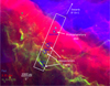 |
Fig. 1 JWST NIRCam composite image of the Orion Bar, located in the Orion molecular cloud (Habart et al. 2024). Red shows the 3.35 μm emission (F335M filter), blue highlights the emission of Paα (F187N filter subtracted by F182M filter), and green indicates the emission of the H2 0–0 S(9) line at 4.70 μm (F470N filter subtracted by F480M filter). The white box represents the field of view of NIRSpec. The blue boxes correspond to the aperture where the spectra are averaged in the three dissociation fronts (DF1, DF2 and DF3). |
2 HD chemistry and excitation
The Meudon PDR code solves the chemical and thermal balance of a plane parallel slab of gas submitted to an external radiation field. A detailed radiative transfer treatment from ultraviolet to infrared photons allows the photodissociation probabilities of several molecules to be computed, including H2, HD and CO from the integration of the state dependent photodissociation cross-sections multiplied by the intensity of the radiation field computed at each point of the 1D structure, while accounting for dust and gas contributions, as explained in the previously cited papers. Here, we solve the statistical equilibrium of the first 52 levels of HD that encompass the v = 2, J = 11 level (highest energy levels at E = 17402.7 K) within the X electronic ground state. The equations are very similar to those describing H2 excitation and they include v, J dependent photodissociation rates resulting from discrete line absorption followed by emission into the continuum of the X electronic ground state as computed by Abgrall & Roueff (2006). The general form of the detailed balance equations can be written as
![Mathematical equation: $\[n_i\left(\sum_{j \neq i} R_{i j}+D_i\right)=\sum_{j \neq i} n_j ~R_{j i}+F_i,\]$](/articles/aa/full_html/2026/01/aa57445-25/aa57445-25-eq1.png) (1)
(1)
where ni is the population of the molecule on level i (in cm−3), Di (in s−1) represents the chemical destruction terms (including photodissociation), Rij and Rji (in s−1) are the transition rates from level i to level j (respectively from level j to level i) including radiative and collisional processes, and Fi (in cm s−3 s−1) is the formation rate of HD into level i. We detail below the main new features of our model.
2.1 Formation and destruction processes
2.1.1 Main reactions
We considered both the gas phase and grain surface reactions that contribute to HD formation, including Langmuir Hinshelwood and Eley–Rideal mechanisms, similarly as what is done for the modeling of H2 (Le Bourlot et al. 2012). We followed Gay et al. (2011) to build the gas phase chemistry of HD, except for the photodissociation mechanism that we computed from the individual photodissociative absorption radiative transitions previously computed by Abgrall & Roueff (2006). HD chemical formation is mainly achieved through reactions of different deuterium-containing species with H2, and destruction is dominated by gas phase reactions with various forms of hydrogen, in addition to photodissociation. The reactions of formation and destruction of HD are those which follow.
Formation:
![Mathematical equation: $\[\mathrm{D}+\mathrm{H}_2 \rightarrow \mathrm{HD}+\mathrm{H} \qquad\qquad E_a=3820 \mathrm{~K}\]$](/articles/aa/full_html/2026/01/aa57445-25/aa57445-25-eq2.png) (2)
(2)
![Mathematical equation: $\[\mathrm{D}^{+}+\mathrm{H}_2 \rightarrow \mathrm{HD}+\mathrm{H}^{+}\]$](/articles/aa/full_html/2026/01/aa57445-25/aa57445-25-eq3.png) (3)
(3)
![Mathematical equation: $\[\mathrm{H}_2 \mathrm{D}^{+}+\mathrm{H}_2 \rightarrow \mathrm{HD}+\mathrm{H}_3^{+} \qquad\qquad \Delta H=-232 \mathrm{~K}\]$](/articles/aa/full_html/2026/01/aa57445-25/aa57445-25-eq4.png) (4)
(4)
![Mathematical equation: $\[\mathrm{D}+\mathrm{H}::~ \rightarrow \mathrm{HD}\]$](/articles/aa/full_html/2026/01/aa57445-25/aa57445-25-eq5.png) (5)
(5)Destruction:
![Mathematical equation: $\[\mathrm{HD}+\mathrm{H} \rightarrow \mathrm{H}_2+\mathrm{D} \qquad\qquad E_a=4240 \mathrm{~K}\]$](/articles/aa/full_html/2026/01/aa57445-25/aa57445-25-eq6.png) (6)
(6)
![Mathematical equation: $\[\mathrm{HD}+\mathrm{H}^{+} \rightarrow \mathrm{H}_2+\mathrm{D}^{+} \qquad\qquad \Delta H=-464 \mathrm{~K}\]$](/articles/aa/full_html/2026/01/aa57445-25/aa57445-25-eq7.png) (7)
(7)
![Mathematical equation: $\[\mathrm{HD}+\mathrm{H}_3^{+} \rightarrow \mathrm{H}_2+\mathrm{H}_2 \mathrm{D}^{+}\]$](/articles/aa/full_html/2026/01/aa57445-25/aa57445-25-eq8.png) (8)
(8)
![Mathematical equation: $\[\mathrm{HD}+h v \rightarrow \mathrm{H}+\mathrm{D}\]$](/articles/aa/full_html/2026/01/aa57445-25/aa57445-25-eq9.png) (9)
(9)
The negative difference of enthalpy variations corresponds to endothermic pathways. Reactions (2) and (6) possess activation barriers Ea that largely overcome the involved enthalpy variations (|ΔH| = 420 K). H:: in reaction (5) stands for H chemisorbed on grains (Le Bourlot et al. 2012), that may react with atomic gas phase deuterium impinging on the chemisorbed site. The neutral-neutral reactions (2) and (6) are specifically taking place in the warm irradiated front of dense and strong PDRs where the high temperature and/or the high excitation of H2 allows to overcome the energy barriers. The ion–molecule reactions occur principally in the more shielded, dense and colder regions and are driven by cosmic rays. Photodissociation is the main destruction route of HD over an extended range of the cloud.
The couples of reactions ((2)–(6), (3)–(7), (4)–(8)) involve forward and reverse competing paths that depend on the excitation state of H2. A more complete discussion is given in Sect. 3.4 and B.2.
2.1.2 State-to-state chemical reactions
The detailed balance equations governing the excitation of a molecule also include chemical formation and destruction processes, that depend on the internal states of the reactants and products. This dependence is usually unknown and is either neglected or treated with educated guesses, which may lead to significant errors in the resulting computed populations and lines intensities.
The two neutral-neutral reactions (2) and (6) have been studied for different rovibrational states of H2 and HD by Bossion et al. (2019) and Bossion et al. (2020) in a state-to-state quasiclassical approach, and we introduced these data into our model1. The state-dependent rate coefficients for reaction (2) include 261 levels of H2 and 398 levels of HD. The rate coefficients for the reverse reaction (6), that involves an activation barrier, use 301 levels of H2 and 239 levels of HD. They provide a remarkable update to the analytic global rate previously recommended by Gay et al. (2011).
We introduced these data into the PDR code for both H2 and HD detailed balance equations and chemical steady-state computation. The impact of using these state-to-state rate coefficients is examined in Appendix B.2. We also account for the dependence on the ortho-to-para ratio of H2 for reaction (4) that becomes significant in the shielded cold part of the cloud. For all other HD formation reactions, we suppose that the newly formed molecules are distributed proportionally to a Boltzmann factor at the gas temperature. State-resolved rates were also calculated for reactions (3) (Honvault & Scribano 2013), (7) (Lepers et al. 2019, 2021), (4) and (8) (Hugo et al. 2009), that occur in the shielded colder region and do not contribute to rovibrational HD emission. Due to the complexity of extrapolating these rates to temperatures and HD levels of interest in this study, we did not implement them and include the ortho/para dependence on H2 in an approximate way. Improvements in modeling are thus expected, thanks to the constant advancements in state-to-state chemistry calculations.
2.2 Excitation and de-excitation processes
2.2.1 Radiative rovibrational transitions within X
A significant difference between HD and H2 is that weak electric dipolar transitions within ![Mathematical equation: $\[X^{1} \Sigma_{g}^{+}\]$](/articles/aa/full_html/2026/01/aa57445-25/aa57445-25-eq10.png) may occur, due to a small dipole moment (8.4 × 10⁻⁴ Debye), resulting from the difference of location of the center of mass and the center of charge of the molecule. Energy levels and radiative transition probabilities of X are taken from Amaral et al. (2019), as found on the HITRAN2 database, updating previous calculations by Abgrall et al. (1982).
may occur, due to a small dipole moment (8.4 × 10⁻⁴ Debye), resulting from the difference of location of the center of mass and the center of charge of the molecule. Energy levels and radiative transition probabilities of X are taken from Amaral et al. (2019), as found on the HITRAN2 database, updating previous calculations by Abgrall et al. (1982).
2.2.2 Ultraviolet electronic radiative transitions
We included the transitions linking the ground state to the four upper electronic states B1 Σu, C1Πu, B′ 1Σu and D 1Πu, where discrete line absorption is followed by discrete and continuous emission. The discrete emitted transitions toward rovibrationally excited levels within the ground state are followed by subsequent infrared radiative cascades that may be detected. On the other hand, transitions toward the continuum lead to photodissociation of the molecule. The formalism closely follows that of H2, as emphasized previously.
2.2.3 Collisions
Different colliders (H, He, H2, H+, electrons) may induce collisional excitation and de-excitation between rovibrational levels belonging to the ground electronic state of HD. We collected the different available collisional data.
Rovibrational collisional excitation rate coefficients with H are taken from the recent computations of Desrousseaux et al. (2022). They are provided up to level v = 2, J = 11 of HD. The rates for collisions with He are taken from Nolte et al. (2012), as found in the UGAMOP3 database. They include 872 transitions from levels up to v = 17, J = 1, but with low J only. The corresponding data for collisions with H2 are taken mostly from Flower & Roueff (1999) except for levels with v = 0, J < 9 where recent results from Wan et al. (2019) are used. Collision rates with H+ come from González-Lezana et al. (2022), as found in the EMAA4 database. Note that many pairs of levels are still missing from these data.
We also considered collisions with electrons that have been approximated by Dickinson & Richards (1975); Dickinson et al. (1977). The suggested expression of the rate coefficient α in cm3 s−1 for low dipole moment values is reported as5
![Mathematical equation: $\[\begin{aligned}\alpha(j \rightarrow j+1)= & \frac{3.56 \times 10^{-6} ~D^2}{\sqrt{T}\left(\frac{2 j+1}{j+1}\right)} \exp (-\beta ~\Delta E) \\& \times \ln \left(C ~\Delta E+\frac{C}{\beta} \exp \left(\frac{-0.577}{1+2 \beta \Delta E}\right)\right)\end{aligned}\]$](/articles/aa/full_html/2026/01/aa57445-25/aa57445-25-eq11.png) (10)
(10)
with
![Mathematical equation: $\[\begin{aligned}& C=\frac{9.08 \times 10^3}{B_0~(j+1)}; \quad \beta=\frac{11~600}{T}; \quad \Delta E=2.48 \times 10^{-4} ~B_0(j+1) \\& D=8.4 \times 10^{-4} \text { Debyes }; \quad B_0=45.655 \mathrm{~cm}^{-1},\end{aligned}\]$](/articles/aa/full_html/2026/01/aa57445-25/aa57445-25-eq12.png)
where ΔE is an energy term expressed in eV whereas C and β are homogeneous to the inverse of energy, expressed in eV−1. Note that Eq. (10) leads to huge variations of α for T < 100 K, that are not critical due to their negligible contribution.
Given the different availabilities, we finally solved the detailed balance equations (1) for the first 52 levels of the X ground state, where the highest energy level is v = 2, J = 11, at 17402.7 K above the ground level. The levels located above that energy are assumed to depend only on radiative processes that are readily computed, following the cascade formalism detailed in van Dishoeck & Black (1986); Viala et al. (1988).
3 A fiducial model
3.1 Parameters
We used version 7 of the Meudon PDR code6, modified to include all processes described in Sect. 2. Ultraviolet Lyman series absorption lines from H, D, as well as Lyman (B-X), Werner (C-X), (B′-X) and (D-X) transitions of H2 and HD were included in the radiative transfer model, as described in Goicoechea & Le Bourlot (2007). Hence all incidental line overlap between these species and self-shielding effects are accounted for straight away. We adopted a base model of the Orion Bar environment following previous PDRs4All publications as displayed in Table 1. Note that a constant pressure model is compatible with steady state.
The cloud is illuminated by the standard isotropic Interstellar Radiation Field (ISRF) plus the O7 type θ Orionis irradiating star (Habart et al. 2023), set at a distance d* = 0.5 pc from the edge of the cloud (based on values given in Pellegrini et al. 2009; O’Dell et al. 2020). We modeled the star spectrum with the Castelli & Kurucz atlas7 (Castelli & Kurucz 2003) for a star with an effective temperature of Teff = 4 × 10⁴ K and log g = 4.5. The effective G0 at the cloud edge, with respect to the standard Habing ISRF reference (Habing 1968), is G0 = 1.4104, in the range of previously suggested values (Joblin et al. 2018). Table A.1 and Fig. A.1 give the correspondence between G0 and d* for different values of d*. The extinction curve was taken from Fitzpatrick & Massa (1988). We took the power law suggested by Mathis et al. (1977) to describe the dust size distribution. The grains composition is a mixture of carbon and silicates as described by Weingartner & Draine (2001). The adopted Line of Sight (LoS) is HD 38087 (Joblin et al. 2018), with RV = 5.5, as prescribed in Habart et al. (2024). We used a relative abundance δD = D/H = 1.5 × 10⁻⁵, representative of the standard elemental ratio (Linsky et al. 2006). A minimal oxygen surface chemistry was included, following Hollenbach et al. (2009).
Fiducial model parameters.
3.2 Structure
Figure 2 shows the temperature and density profiles of the relevant regions of the cloud edge. Five zones, corresponding to five different regimes are defined and used subsequently, as described below.
Zone I extends from the ionization front to an abrupt drop in the temperature profile. As shown below (Sect. 3.3), the transition from zone I and zone II is the point where H2 collisional excitation followed by radiative decay turns from a heating to a cooling process when collisions become more efficient due to the higher density.
Zone II is partially atomic, and exhibits a rising amount of molecular gas up to the location where atomic and molecular hydrogen abundances are equal. Efficient self-shielding in H2 absorption transitions is taking place and allows some molecules to form. This zone extends also to the point where atomic and molecular deuterium abundances become equal.
Zone III starts at the position where n(H2) = n(H), beyond which the gas is mostly molecular.
Zone IV begins at the transition from C+ to CO as the dominant carbon bearing species. It marks the beginning of the molecular region of the PDR for all species. Deuterium exchange reactions
![Mathematical equation: $\[\mathrm{HD}+\mathrm{H}_{3}^{+} \rightleftarrows \mathrm{H}_{2} \mathrm{D}^{+}+\mathrm{H}_{2}\]$](/articles/aa/full_html/2026/01/aa57445-25/aa57445-25-eq14.png) take place in zone IV, allowing formation of further deuterated compounds (DCO+, ...).
take place in zone IV, allowing formation of further deuterated compounds (DCO+, ...).Zone V is a high density, low temperature, dark molecular environment where reactions in ice mantles play a dominant role. It is not relevant for our study.
The sizes of zones I, II, III and IV are respectively dI = 4.5 × 10⁻², 0.64 × 10⁻², 0.43 × 10⁻² and 0.54 × 10⁻² pc, (equivalently ~9200, 1300, 900 and 1100 au), with the parameters reported in Table 1.
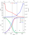 |
Fig. 2 Variations of temperature, density and abundances as a function of distance from the ionization front, d, and visual extinction, AV, for the fiducial model. See Sect. 3.2 for the definitions of zones I to V. (a) Temperature (red line, left axis) and density profiles (blue line, right axis). (b) Relative abundances of H and H2, (resp. D and HD), normalized by n(H) + n(H2) (resp. n(D) + n(HD)). Values at the transitions are given in Table 2. |
Transition values.
3.3 Heating and cooling processes
Figure 3 shows the main heating and cooling processes of the gas. We assume thermal balance, so the total heating and cooling rates are equal. Unsurprisingly the main heating process at the cloud edge is photo-electric effect on dust. However, two other processes have a significant contribution, namely radiative cascades and chemical reactivity.
In zone I, the radiative pumping of H2 followed by collisional deexcitation is important. This may come as a surprise, since the abundance of H2 is negligible here. But since H2 photodissociation occurs in discrete transitions, with a dissociating probability of about 10%, nine times out of ten, absorption of an ultraviolet photon is followed by a radiative cascade to an excited vibrational state. The subsequent deexcitation results from a competition between collisional and radiative decay. Collisional de-excitation increases the kinetic energy of the gas and takes place in this front, medium density, warm zone.
In zone II, self-shielding of H2 proceeds and collisional excitation followed by radiative emission is now a cooling process (since kinetic energy is transferred into radiation). H2 abundance is also high enough for an active chemistry to take place and exothermic reactions contribute to heating. Appendix C details these processes.
H2 formation on grains through the Eley-Rideal process has a minor contribution to gas heating (~10%). Cooling is dominated by far-infrared [O I] fine-structure lines, but here also it is not the only process to participate in the cooling. Everywhere up to the molecular core, gas-grain collisions contribute to about 10%. Once H2 survives in a significant amount (zone II), it contributes to more than 30%, and deeper into the cloud, CO and its isotopes contribute to about 40%. C+ has a minor contributions up until the molecular core (less than 4% everywhere). Other species (C, OH, H2O, ...) are completely negligible.
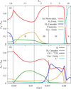 |
Fig. 3 Main contributions to (a) heating (Γ) and (b) cooling (Λ) of the gas as a function of distance d from the ionization front and visual extinction, AV. Each heating (resp. cooling) term is normalized by the total heating/cooling. |
3.4 HD abundance
HD formation starts as soon as some molecular H2 is available, through the D + H2 reaction. Fig. 5 shows the relative role of reactions (2)–(9) normalized by the total formation rate. In panel a, individual reaction rates are shown, whereas in panel b, the sum of forward and reverse processes is shown, which helps to identify the main mechanisms.
Photodissociation is the major destruction channel of HD up to the middle of zone III, as shown in panel b. We carefully consider the different possible overlap of HD, H, D and H2 UV transitions as well as self-shielding effects of H2 and HD dissociating transitions. We show an example in Fig. 4 where a small portion of the radiative energy density uλ is displayed at AV = 1.7 (d ≃ 0.05 pc, just before zone III). Absorption lines in blue come from H2. HD lines are shown in red. Two lines arising from v = 0, J = 2 are identified. The 14–0 R(2) line is only mildly shielded, whereas the 14–0 P(2) line falls in the wing of a strong H2 line, impacting the dissociation efficiency. We also note the presence of the strong 14–0 R(1) transition in the wavelength range. Compared to the simple Federman et al. (1979) approximation of the self-shielding, detailed account of the self-shielding and line overlapping reduce photodissociation by 10–30% over zone II.
Diverse chemical processes occur in the dense zones III and IV, where the temperature gradually decreases from ~600 K down to 50 K. The transition between zone III and IV corresponds to the position where the role of neutral-neutral reactions involving energy barriers is progressively declining whereas ion-molecule reactions become important. The Eley-Rideal HD formation process on grains dominates over a small spatial range before reactions with H2D+ take over. We note that photodissociation remains significant in zone III and a large part of zone IV. Appendix B.2 gives more details.
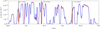 |
Fig. 4 Radiative energy density uλ at AV ~ 1.7 (d = 0.05 pc) in the 96–96.3 nm far ultraviolet wavelength range. Blue indicated H2 lines, while red shows HD lines. The positions of three strong HD absorption lines are shown using black vertical lines, coming from v = 0, J = 1 and J = 2. |
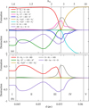 |
Fig. 5 Relative contribution of HD formation and destruction reactions normalized to the total formation rate. (a): Individual reactions (2)–(9). (b) Sum of direct and reverse reactions. The y-axis is dimensionless. |
3.5 HD excitation
Figure 6 shows where, in the PDR, excited levels of HD are found. Beyond zone III only the lowest levels of the ground vibrational mode J = 0 and 1 are populated. The lines within v = 0 come mostly from zone III, while excited vibrational levels come from zone II, with a well-defined separation between both. So HD vibrational emission comes from a region where H2 is still a minor component, but is subject to enhanced vibrational excitation, as shown in Fig. C.2.
We compute the full emission spectrum as seen by an external observer, including HD lines and also all lines from species participating in the cooling of the gas (H2, O, ...) and included in our model. HD lines from v = 2 levels are weaker than lines from v = 1 levels by about a factor of 3. This is confirmed by the excitation diagram shown in Fig. 7: the v = 2 branch is below the v = 1 one. As the product hν × N(J) × Aul (where Aul is the Einstein emission coefficient) is very similar for v = 2 → 1 transitions compared to v = 1 → 0 transitions, the difference can be attributed to differences in column densities (See Appendix B.1 for details and Fig. 12 for an example spectrum).
An excitation temperature Tex can be derived for each vibrational ladder of the excitation diagram. To compare these excitation temperatures to the gas kinetic temperature, we compute a “vibrationally weighted” mean gas kinetic temperature ![Mathematical equation: $\[T_{kin}^{v}\]$](/articles/aa/full_html/2026/01/aa57445-25/aa57445-25-eq15.png) by
by
![Mathematical equation: $\[T_{k i n}^v=\int_0^{d_{max }} T(s) ~n_v(s) ~d s / \int_0^{d_{max }} n_v(s) ~d s,\]$](/articles/aa/full_html/2026/01/aa57445-25/aa57445-25-eq16.png) (11)
(11)
where T(s) is the gas kinetic temperature at position s, nv(s) is the abundance in cm−3 of HD in vibrational level v (summed over all rotational levels) and dmax is the size of the PDR. Results are given in Table 3. The excitation temperatures are close to the “vibrationally weighted” mean gas kinetic temperature for v = 0, but significantly different for excited v.
To understand the difference between v = 0 and v > 0 excitation, we explore the different excitation processes by developing the various Rji terms in the statistical equilibrium equations (1). The relative weight of each process can be assessed by computing the balance of formation and destruction of molecules in a given level i due to each one. We define
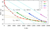 |
Fig. 7 Full modeled excitation diagram for HD. Light blue lines indicates fits to lowest J for each v giving the indicated excitation temperatures Tex, light golden lines shows fits to high J giving a |
![Mathematical equation: $\[T_{e x}^{\text {high} ~J}\]$](/articles/aa/full_html/2026/01/aa57445-25/aa57445-25-eq20.png)
![Mathematical equation: $\[S_i^e=\sum_j x_j R_{j i}^e,\]$](/articles/aa/full_html/2026/01/aa57445-25/aa57445-25-eq21.png) (12)
(12)
where xj is the relative population of HD in level j. e stands for either r: radiative quenching transitions, c: collisions transitions, p: radiative pumping and cascades or f: formation excitation. The various terms are expressed in s−1.
Figure 8 shows the four processes, at AV ~ 1.7 (d = 0.05 pc) for the considered J values belonging to v = 0 and v = 1. In the case of v = 0, the dominant terms in the detailed balance equations (1) come from collisions with H2 and H and spontaneous radiative de-excitation. v = 0 levels peaks in zone III, where the density is high enough, so collisions are efficient enough to bring the excitation temperature close to the kinetic temperature. For v = 1, the populations mainly result from radiative pumping balanced by spontaneous radiative emission up to J = 7 (see Fig. 8, panel c). Then collisions and formation excitation progressively take over. This is due to the fact that radiative transitions can change J by at most 1 unit, whereas a single collision may lead to a large change in J. Over zone II collisions are dominated first by H, while H2 becomes progressively as competitive. The excitation of HD v > 0 low-J due to FUV-pumping is subthermal (![Mathematical equation: $\[T_{\mathrm{ex}}<T_{kin}^{v}\]$](/articles/aa/full_html/2026/01/aa57445-25/aa57445-25-eq22.png) ) because of the small HD electric dipole moment allowing electric dipolar transitions. For instance, level v = 1, J = 10 of HD has an inverse radiative lifetime 158 times higher than the same level of H2, with the main contribution coming from the electric dipole R(9) transition with an Einstein coefficient of 7.65 × 10⁻⁵ s−1.
) because of the small HD electric dipole moment allowing electric dipolar transitions. For instance, level v = 1, J = 10 of HD has an inverse radiative lifetime 158 times higher than the same level of H2, with the main contribution coming from the electric dipole R(9) transition with an Einstein coefficient of 7.65 × 10⁻⁵ s−1.
We note also that for each vibrational branch in Fig. 7 the highest J levels follow a higher temperature (last line of Table 3, and brown lines on the figure). This change of slope coincides with the begining of the next v branch, which suggests a coupling between v and v + 1 levels. This was confirmed by a careful examination of formation and destruction processes of high J levels: collisional decay from v + 1 to v with ΔJ ⩾ 2 is efficient enough to lead to an overpopulation of these levels compared to populations expected from the cold component.
A list of line intensities is given in Appendix E for rotational transitions, and transitions with Δv = 1, 2 and 3. Most of these lines are not seen in the current spectra (see next Section), but the quoted intensities show which noise level must be reached in order to detect them.
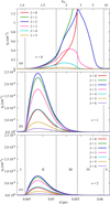 |
Fig. 6 Hydrogen deuteride excited rotational levels abundance profiles as a function of distance from the ionization front, d, and visual extinction, AV. (a) v = 0 (top panel), (b) v = 1, (c) v = 2. See Fig. C.2 for a comparison with H2. |
Excitation and vibrationally weighted kinetic temperatures.
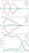 |
Fig. 8 Excitation balance |
![Mathematical equation: $\[S_{j}^{e}\]$](/articles/aa/full_html/2026/01/aa57445-25/aa57445-25-eq23.png)
4 Observations
4.1 Data reduction
We used the observations of the NIRSpec integral field unit (IFU) mode from the Early Release Science (ERS) program PDRs4All8: radiative feedback from massive stars (ID1288, PIs: Berné, Habart, Peeters, Berné et al. 2022). NIRSpec observations cover a 9 × 1 mosaic (NIRspec’s field of view being 3″ × 3″) centered on αJ2000 = 05h35min20.4749s, δJ2000 = −05°25′10.45″. We used the full spectro-imaging cubes9. The data were reduced using the JWST science pipeline (version 1.16.0) and the context jwst_1295.pmap of the Calibration References Data System (CRDS) (see Peeters et al. (2024) for observation parameters and data reduction process). The world coordinate system (WCS) of the cubes were corrected by measuring the coordinates of the proplyd d203-506, and then computing the offset between the centroid of this proplyd in synthetic F212N images (NIRSpec data integrated over NIRCam filter F212N) and the manually set coordinate values. The same shift was applied to all three NIRSpec channels. We also use the average spectrum extracted over the apertures given by Peeters et al. (2024), Chown et al. (2024) and Van De Putte et al. (2024) for the Bar (see Fig. 1). These spectra are in units of MJy sr−1.
Analyzing faint HD lines, we noticed that updates in the data reduction pipeline and reference files have affected the measurements, and in particular, there were previous versions of our reduced data where some lines were no longer detected (for instance, the 1–0 R(3) line). It is very difficult to precisely assign the origin of this effect observed on the spectra but this is probably linked to the reference files (hence the dark and flat used) which have evolved since the commissioning. The most recent data reduction provides the cleanest spectrum and does not seem affected by these effects. However, further investigation is needed and is out of the scope of this paper.
As the HD rovibrational emission is detected in the NIR, it can be affected by extinction along the line of sight. We need to correct HD emission for attenuation by the matter inside the PDR and the foreground matter in the line of sight, that is different from the extinction by the matter inside the PDR toward θ1 Ori C, which is negligible at the H/H2 transition (AV < 2) (see Fig. 14 of Peeters et al. (2024) and Fig. 5 of Habart et al. (2024)). In order to do that, we use the R(V)-parameterized average Milky Way curve by Gordon et al. (2023) (Gordon et al. 2009; Fitzpatrick et al. 2019; Gordon et al. 2021; Decleir et al. 2022), for an R(V) = 5.5 following Peeters et al. (2024) and Van De Putte et al. (2024). In the third dissociation front (DF3), the extinction in the line of sight is estimated to be around AV = 3.4, as derived by summing the extinction determined for the foreground (AV = 1.4) and that intrinsic to the atomic PDR (AV = 2). In DF2, using the same extinction curve, the extinction is estimated to be around AV = 5.87. One should note that the extinction curve defined in Gordon et al. (2023) is not sufficient to explain the observations in the Orion Bar (Meshaka et al., in prep.). However, the relevant wavelength range of detected HD lines is very narrow (2.5–3.0 μm), leading to a negligible impact on the results of this study compared to other sources of uncertainties.
4.2 Detection and spatial morphology
Hydrogen deuteride rovibrational lines are detected in several regions of the Orion Bar, mainly in the three dissociation fronts. Fig. 9 displays the spectra where HD lines are detected. In total, we detect 7 rovibrational lines v = 1 → 0 in DF2 and DF3, from R(0)–R(3) and P(1)–P(3). Fewer lines are detected in the DF1 (only R(1)–R(3)), probably due to the higher extinction toward this front (AV ~ 10), a result of the terrace-field like structure (Habart et al. 2024; Peeters et al. 2024). Due to high continuum in the Orion Bar, fringes lead to high noise levels beyond 15 μm, no pure rotational lines of HD are detected. To derive the absolute intensities of HD lines, we fit the observed lines with a Gaussian coupled with a linear function to take into account the continuum and then integrated the Gaussian function over the wavelengths. When necessary, a fit of two gaussians was made for HD lines which were blended (e.g., 1–0 P(1), 1–0 R(3)). The upper limit of intensities are calculated by considering two times the noise level on the continuum. Column densities in the upper level of each transition are calculated as follow
![Mathematical equation: $\[N_{\mathrm{up}}=4 \pi \frac{I}{A_{i j}} \frac{\lambda}{h c},\]$](/articles/aa/full_html/2026/01/aa57445-25/aa57445-25-eq24.png) (13)
(13)
where I is the integrated intensity10 of the line (erg cm−2 s−1 sr−1), λ the wavelength of the transition (μm), Aij the Einstein coefficient of the transition (s−1), h the planck constant and c the velocity of light. Column densities from different lines coming from the same upper level are combined according to the expressions of Appendix D.2. As the lines in DF1 are very faint, we exclude them for the rest of this paper. Integrated intensities of the lines and column densities of the levels observed in DF3 and DF2 are presented in Table 4.
Figure 10 displays the normalized integrated intensity profiles of HD and H2 lines around DF 3. It shows that HD and H2 rovibrational emission coincide, slightly closer to the edge of the cloud than the pure rotational lines of H2.
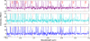 |
Fig. 9 NIRSpec continuum-subtracted observed spectrum. The dashed vertical red lines are the position of the first rovibrational v = 1 → 0 HD lines. From top to bottom, this figure shows the spectrum of the dissociation fronts of the Orion Bar: DF1, DF2, DF3. The apertures taken to average these spectra are from Peeters et al. (2024) for the dissociation fronts. These spectra are not corrected for extinction. |
4.3 Excitation
Figure 11 displays the rotational diagrams of detected rovibrational HD lines in DF3 and DF2. In DF3, we can properly derive the column densities of five levels, which allows to derive an excitation temperature of Tex ≃ 484 ± 54 K following
![Mathematical equation: $\[\ln \left(\frac{N_{\mathrm{up}}}{g_{\mathrm{up}}}\right)=\ln \left(\frac{N}{Q\left(T_{\mathrm{ex}}\right)}\right)-\frac{E_{\mathrm{up}}}{k_{\mathrm{B}} T_{\mathrm{ex}}},\]$](/articles/aa/full_html/2026/01/aa57445-25/aa57445-25-eq25.png) (14)
(14)
In DF2, fewer lines can be adequately measured, and hence the excitation temperature is badly constrained. However, the range of derived values of Tex ≃ 708 ± 248 K encompasses the value derived in DF3.
Here, the uncertainty is only calculated based on the measurement of HD line integrated intensities. The detected lines are very weak and so their integrated intensities have large error bars, which is the main cause of uncertainties. However, other factors could affect the estimation of the excitation temperature. First, the correction for extinction could affect the line ratios of HD and thus the derived excitation temperature. Using Eq. (D.3) of Appendix D.1, the relative uncertainty on the temperature induced by the limited knowledge of the extinction is at most a few percent, due to the narrow wavelength range. The second factor which can greatly affect the excitation temperature is the uncertainty on integrated intensities due to data reduction effects, as discussed in Sect. 4.1. These effects seem to reduce the intensity of detected lines which lead to large relative uncertainties for weak lines. As we are only detecting a few levels, the absolute intensities of each transition have a great impact on the derived excitation temperature. For instance, if the intensity of the 1–0 R(3) line is underestimated due to data reduction effects, the derived excitation temperature will be higher.
Figure 11 shows that the five weighted column densities are very well aligned, pointing to the conclusion that the excitation temperature is most likely around 500 K. However, due to the small number of lines used to derive the temperature and the impact of data reduction discussed above, we cannot firmly ignore the possibility of a slightly higher or colder excitation temperature. Using the spectra of DF2 and DF3, where we expect the same HD excitation, the excitation temperature seems to vary between Tex ~ 480–710 K. To be conservative, we also use this range of values to compare with PDR models.
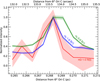 |
Fig. 10 Normalized integrated intensity profiles of the HD 1–0 R(0) line, H2 0–0 S(1) line, and H2 1–0 S(1) line across the third dissociation front DF 3 as a function of the projected distance to the star Θ1 Ori C. The distance to the Orion Bar used to calculate the distance to the star in arcsec is d = 414 pc (Menten et al. 2007). Each point corresponds to the intensity averaged on apertures with width of 2.5″ and height of 0.4″ with an angle of 38° (to match DF3 orientation) to increase the S/N. |
Integrated intensities and upper level column densities of HD observed rovibrational lines in DF2 and DF3.
5 Comparison between models and observations
In this section, we discuss to what extent the fiducial model can reproduce the observations and if HD can be used to constrain physical parameters of PDRs.
5.1 Comparison with the fiducial model
Overall, the predictions of the fiducial model described in Sect. 3 are compatible with representative features of HD observations, such as the location of the HD emission and its excitation. Indeed, the model establishes that formation of HD occurs as soon as some H2 is available, in zone II, and that deuterium becomes fully molecular slightly before hydrogen as shown in Fig. 2. That zone corresponds to the maximum of vibrational excitation favored by efficient ultraviolet pumping followed by radiative cascades into excited vibrational levels. The model can also account for the excitation of HD in this region. Indeed, the model predicts an excitation temperature Texmodel ~ 600 K, only marginally higher than what is observed Texmodel ~ 500 K.
Figure 12 shows a comparison of the modeled and observed spectrum for P = 5 × 10⁷ K cm−3 and d* = 0.5 pc, with line identification. The theoretical spectrum is computed at an angle of 70° with respect to the normal of the cloud to account for the fact that the various dissociation fronts are seen almost edge on (see Fig. 1). This angle is chosen to best fit the observed column density. Fig. 13 shows the observational and theoretical excitation diagrams for the detected levels of v = 1. Theoretical values have been scaled by a factor 1/ cos (70°) here. Given the large sources of uncertainties (See Sect. 4) and the fact that the front is certainly not straight, the agreement is satisfactory.
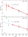 |
Fig. 11 Excitation diagram of HD rovibrational lines in the DF3 (a) and the DF2 (b). The arrows correspond to the upper limits of HD lines which cannot be properly measured. The solid lines correspond to the fit to the distribution. The y-axis scales are identical to allow a visual comparison of Tex. |
5.2 HD as a tracer of physical conditions in the Orion Bar
The underlying question is whether HD rovibrational emission can be used as a valuable tracer of physical conditions in PDRs. In order to find the constraints that HD can provide, we explore a range of physical parameters. With respect to Sect. 3, we keep all parameters fixed, except the pressure P and the intensity of the UV field G0. As we focus on constraining the physical conditions in the PDR, we can exclude, as fit parameters, AV which is not relevant for HD lines emitted in a surface layer. We also exclude the extinction properties which are related to the material composition. We checked the importance of the cosmic ray ionization rate by increasing its value by a factor 1000. Due to the increase of temperature near the edge, and hence a decrease of density, the atomic to molecular transition is significantly shifted toward larger values of AV, leading to an increase of zone I size by a factor of about 4, which does not comply with the present observations. HD chemistry at the rovibrational emission peak is still dominated by UV-driven chemistry (dominated by reactions (2) and (9)). The column density of HD is only slightly lower and the excitation temperature of HD rovibrational levels is marginally affected, below the observational uncertainties. Hence, we chose to exclude ζ as a fit parameter. In order to constrain a best-fit model for the Orion Bar, we consider a few pairs of parameter values, with a thermal pressure from P = 3 × 10⁷ to 108 K cm−3 and G0 from ~0.7 × 10⁴ to ~4 × 10⁴ (by varying the distance to the star d* = 0.3–0.7 pc).
To compare with observations, we selected two quantitative constraints from the data, which are
The distance D between the ionization front and the rise of H2 emission. We adopted a value of D = 3.8 ± 1.0 × 10⁻² pc as discussed in Habart et al. (2024). In the model, this is dI, the size of zone I.
The HD excitation temperature derived from v = 1. In Sect. 4, we get Tex = 484 ± 54 K. As discussed in Sect. 4.3, due to data reduction effects on line intensities and the uncertainties on extinction correction, we cannot firmly rule out the possibility of a slightly higher or colder excitation temperature. To be conservative, we also also considered a range of values from Tex = 480–710 K to compare to models.
Figure 14 shows the computed values of dI, and Fig. 15 the computed values of Tex as a function of thermal pressure. The size of zone I decreases with the thermal pressure because the steeper the density gradient is, the closer to the edge H2 and HD are formed. Fig. 14 shows that the observational constraint on the size of zone I implies that the thermal pressure lies between P = (3–9) × 107 K cm−3. Tex depends only weakly on the radiation field intensity and is mainly a function of P. Hence, the present HD observations do not strongly constrain the intensity of the UV field. The observed excitation temperature in DF3 around Tex = 484 ± 54 K sets an upper limit to P ⩽ 3 × 107 cm−3 K. However, if we consider the range of temperature Tex = 480–710 K, models with pressure ranging from P = (2–9) × 107 K cm−3 can reproduce the observed excitation temperature. Considering both limitations, and being conservative with the comparison between modeled and observed excitation temperature, a range of P = (3–9) × 107 K cm−3, with no strict boundary on the intensity of the UV field G0, best reproduce present HD observations.
This result shows that, due to the great uncertainty of HD lines intensities and hence excitation temperature, current HD observations do not provide strong constraints on physical parameters of the Orion Bar. However, the derived range of pressures is in agreement with the latest estimation, P ~ 5 × 10⁷ Kcm−3, obtained from H2 observations with JWST (Meshaka et al., in prep.), which emits in the same region. This new evaluation is lower than the previous value P ~ 2 × 10⁸ K cm−3, derived in the Orion Bar with other tracers observed mainly through rotationally excited transitions of H2, CO, OH, CH+, ... with Herschel at lower spatial resolution (e.g., Joblin et al. 2018). The range of values obtained from different tracers may result from a density and pressure gradient inside the PDR, as already mentioned in Joblin et al. (2018). Indeed, the tracers observed by Herschel rather come from zone III where collisional excitation is most efficient. Interestingly, Goicoechea et al. (2025) find an in between value of thermal pressure (P = 108 K cm−3) in the C2H emitting regions, which is close to the H2 emission. We emphasize that we do not try to derive the relative D/H elemental abundance ratio, that would affect the absolute column density values as well.
6 Conclusions
In this work, we have presented a detailed chemical modeling of the radiation induced D/HD transition including rovibrationally excited HD in a plane parallel slab of gas and dust. We updated the Meudon PDR code to include the contribution of rovibrational excitation processes (collisions, UV pumping, state-to-state chemical reactions, ...) thanks to recently available molecular data. We also carefully reanalyzed the observed rovibrational HD emission lines that were detected by JWST, thanks to its high sensitivity and spatial resolution, toward the Orion Bar (Peeters et al. 2024), and derived a comprehensive excitation diagram. A fiducial isobaric model with physical parameters which best reproduces other tracers (such as H2) satisfactorily compares with the observations. The main conclusions of this study can be summarized as follows:
In this dense environment and intense UV radiation field conditions, the deuterium molecular reservoir HD is closely linked to the formation of molecular gas and is formed in the gas phase via D + H2 = HD + H;
Rovibrational emission of HD is predicted to peak in a zone where the gas is still partially atomic. Alternatively, purely rotational emission of HD reaches its maximum deeper in the cloud, after the H/H2 transition. Hence, these two emissions trace different regions of the PDR. These predictions are in broad agreement with observations of HD rovibrational lines peaking where vibrationally excited H2 is bright, close to the dissociation front. The detailed comparison of the involved length scales is beyond the present study;
The state-to-state reaction rate coefficients for the D + H2 ↔ H + HD reactions have been introduced into a PDR model thanks to detailed theoretical computations (Bossion et al. 2019; Bossion et al. 2020). This achievement allows to confirm the role of vibrationally excited H2 in the formation of vibrationally excited HD in this strong PDR environment, as previously emphasized for the detection of CH+, SH+, NH (Agúndez et al. 2010; Goicoechea & Roncero 2022);
The excitation diagram derived from the five observed levels of HD (v = 1, J = 0–4) gives an excitation temperature close to Tex ~ 500 K. This temperature, however, is rather uncertain due to the faintness of the transitions, resulting in low signal to noise, and a limited number of detected levels. Data reduction effects may also affect the measured intensity of the faintest observed lines. A conservative range of observationally derived excitation temperatures is Tex = 480–710 K, based on the hypothesis that DF2 and DF3 have similar excitation conditions;
We find that models with a range of pressure P = (3–9) × 107 K cm−3 are compatible with observations. This range of values is in agreement with the latest estimation of the thermal pressure in the Orion Bar derived from the analysis of H2 emission (Meshaka et al., in prep.). This range of pressure is lower than the previously derived value from rotational spectra of H2, CO, ... that arise in a different zone of the PDR, suggesting the occurrence of a pressure gradient;
The study of HD is not sufficient to constrain the incident UV field as the excitation temperature of HD rovibrational lines only depends weakly on this parameter;
The models also predict that the excitation temperature of HD rotational emission is close to the gas temperature at the peak position, whereas the excitation of rovibrational levels is subthermal. This may be explained by the major contribution of collisional excitation for rotational levels whereas rovibrational levels are mostly populated by UV radiative pumping followed by the IR cascade.
Our model of the first detected rovibrational lines of HD provides a unique opportunity to undertake a comprehensive survey of physical processes at work in the molecule formation and excitation. It also allows to review in details the transition from the hot atomic layer to the dense molecular inner region. Deeper observations are necessary to detect HD lines with better signal to noise ratio and to map their emission in order to precisly constrain the thermal pressure toward the D/HD and H/H2 transitions.
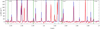 |
Fig. 12 Comparison of observational (red) and theoretical (blue) spectra. The vertical dash-dotted lines indicate lines of H2. The vertical cyan and pink lines indicate recombination lines of H and He respectively. The vertical green lines show the location of HD transitions. The theoretical spectrum is computed for an angle of view of 70°. |
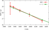 |
Fig. 13 Comparison of observational (in red) and theoretical (in green) excitation diagrams for v = 1. Theoretical column densities have been computed for an angle of view of 70°. |
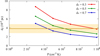 |
Fig. 14 Size of zone I for PDR models at different thermal pressure and UV field intensity (scaled by the distance to the star). |
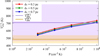 |
Fig. 15 Excitation temperature for v = 1 for various values of P and d*. The observational range of excitation temperatures is displayed as a colored band: yellow for DF3 and purple for DF2. |
Acknowledgements
This work is based [in part] on observations made with the NASA/ESA/CSA James Webb Space Telescope. The data were obtained from the Mikulski Archive for Space Telescopes at the Space Telescope Science Institute, which is operated by the Association of Universities for Research in Astronomy, Inc., under NASA contract NAS 5-03127 for JWST. These observations are associated with program ERS1288. This work was supported by the Thematic Action “Physique et Chimie du Milieu Interstellaire” (PCMI) of INSU Programme National “Astro”, with contributions from CNRS Physique & CNRS Chimie, CEA, and CNES. M.Z. and J.R.G. thank the Spanish MCINN for funding support under grant PID2023-146667NB-I00. M. Z. acknowledges the Juan de la Cierva Postdoctoral Fellow project JDC2024-054658-I, funded by MICIU/AEI/10.13039/501100011033 and by the ESF+. E.P. acknowledges support from the University of Western Ontario, the Canadian Space Agency (CSA, 22JWGO1-16), and the Natural Sciences and Engineering Research Council of Canada.
References
- Abgrall, H., & Roueff, E. 2006, A&A, 445, 361 [NASA ADS] [CrossRef] [EDP Sciences] [Google Scholar]
- Abgrall, H., Roueff, E., & Viala, Y. 1982, A&AS, 50, 505 [NASA ADS] [Google Scholar]
- Agúndez, M., Goicoechea, J. R., Cernicharo, J., Faure, A., & Roueff, E. 2010, ApJ, 713, 662 [Google Scholar]
- Amaral, P. H. R., Diniz, L. G., Jones, K. A., et al. 2019, ApJ, 878, 95 [NASA ADS] [CrossRef] [Google Scholar]
- Atkins, P., de Paula, J., & Friedman, R. 2009, Quanta, Matter, and Change: A Molecular Approach to Physical Chemistry (OUP Oxford) [Google Scholar]
- Berné, O., Habart, É., Peeters, E., et al. 2022, PASP, 134, 054301 [CrossRef] [Google Scholar]
- Bertoldi, F., Timmermann, R., Rosenthal, D., Drapatz, S., & Wright, C. M. 1999, A&A, 346, 267 [NASA ADS] [Google Scholar]
- Bossion, D., Scribano, Y., & Parlant, G. 2019, JCP, 150, 084301 [Google Scholar]
- Bossion, D., Ndengué, S., Meyer, H.-D., Gatti, F., & Scribano, Y. 2020, J. Chem. Phys., 153, 081102 [Google Scholar]
- Bron, E., Le Bourlot, J., & Le Petit, F. 2014, A&A, 569, A100 [NASA ADS] [CrossRef] [EDP Sciences] [Google Scholar]
- Castelli, F., & Kurucz, R. L. 2003, in IAU Symposium, 210, Modelling of Stellar Atmospheres, eds. N. Piskunov, W. W. Weiss, & D. F. Gray, A20 [Google Scholar]
- Caux, E., Ceccarelli, C., Pagani, L., et al. 2002, A&A, 383, L9 [NASA ADS] [CrossRef] [EDP Sciences] [Google Scholar]
- Chown, R., Sidhu, Ameek, Peeters, Els, et al. 2024, A&A, 685, A75 [NASA ADS] [CrossRef] [EDP Sciences] [Google Scholar]
- Decleir, M., Gordon, K. D., Andrews, J. E., et al. 2022, ApJ, 930, 15 [NASA ADS] [CrossRef] [Google Scholar]
- Desrousseaux, B., Coppola, C. M., & Lique, F. 2022, MNRAS, 513, 900 [Google Scholar]
- Dickinson, A. S., & Richards, D. 1975, J. Phys. B At. Mol. Phys., 8, 2846 [Google Scholar]
- Dickinson, A. S., Phillips, T. G., Goldsmith, P. F., Percival, I. C., & Richards, D. 1977, A&A, 54, 645 [NASA ADS] [Google Scholar]
- Federman, S. R., Glassgold, A. E., & Kwan, J. 1979, ApJ, 227, 466 [NASA ADS] [CrossRef] [Google Scholar]
- Ferlet, R., André, M., Hébrard, G., et al. 2000, ApJ, 538, L69 [Google Scholar]
- Fitzpatrick, E. L., & Massa, D. 1988, ApJ, 328, 734 [NASA ADS] [CrossRef] [Google Scholar]
- Fitzpatrick, E. L., Massa, D., Gordon, K. D., Bohlin, R., & Clayton, G. C. 2019, ApJ, 886, 108 [Google Scholar]
- Flower, D. R., & Roueff, E. 1999, MNRAS, 309, 833 [NASA ADS] [CrossRef] [Google Scholar]
- Francis, L., van Dishoeck, E. F., Caratti o Garatti, A., et al. 2025, A&A, 694, A174 [NASA ADS] [CrossRef] [EDP Sciences] [Google Scholar]
- Gay, C. D., Stancil, P. C., Lepp, S., & Dalgarno, A. 2011, ApJ, 737, 44 [Google Scholar]
- Godard, B., & Cernicharo, J. 2013, A&A, 550, A8 [NASA ADS] [CrossRef] [EDP Sciences] [Google Scholar]
- Goicoechea, J. R., & Le Bourlot, J. 2007, A&A, 467, 1 [NASA ADS] [CrossRef] [EDP Sciences] [Google Scholar]
- Goicoechea, J. R., & Roncero, O. 2022, A&A, 664, A190 [NASA ADS] [CrossRef] [EDP Sciences] [Google Scholar]
- Goicoechea, J. R., Pety, J., Cuadrado, S., et al. 2025, A&A, 696, A100 [NASA ADS] [CrossRef] [EDP Sciences] [Google Scholar]
- Gonzalez Garcia, M., Le Bourlot, J., Le Petit, F., & Roueff, E. 2008, A&A, 485, 127 [NASA ADS] [CrossRef] [EDP Sciences] [Google Scholar]
- González-Lezana, T., Hily-Blant, P., & Faure, A. 2022, J. Chem. Phys., 157, 214302 [Google Scholar]
- Gordon, K. D., Cartledge, S., & Clayton, G. C. 2009, ApJ, 705, 1320 [NASA ADS] [CrossRef] [Google Scholar]
- Gordon, K. D., Misselt, K. A., Bouwman, J., et al. 2021, ApJ, 916, 33 [NASA ADS] [CrossRef] [Google Scholar]
- Gordon, K. D., Clayton, G. C., Decleir, M., et al. 2023, ApJ, 950, 86 [CrossRef] [Google Scholar]
- Habart, E., Le Gal, R., Alvarez, C., et al. 2023, A&A, 673, A149 [NASA ADS] [CrossRef] [EDP Sciences] [Google Scholar]
- Habart, E., Peeters, E., Berné, O., et al. 2024, A&A, 685, A73 [NASA ADS] [CrossRef] [EDP Sciences] [Google Scholar]
- Habing, H. J. 1968, Bull. Astron. Inst. Netherlands, 19, 421 [Google Scholar]
- Herráez-Aguilar, D., Jambrina, P. G., Menéndez, M., et al. 2014, Phys. Chem. Chem. Phys. (Incorp. Faraday Trans.), 16, 24800 [Google Scholar]
- Hierl, P. M., Morris, R. A., & Viggiano, A. A. 1997, J. Chem. Phys., 106, 10145 [Google Scholar]
- Hollenbach, D. J., & Tielens, A. G. G. M. 1997, ARA&A, 35, 179 [Google Scholar]
- Hollenbach, D., Kaufman, M. J., Bergin, E. A., & Melnick, G. J. 2009, ApJ, 690, 1497 [NASA ADS] [CrossRef] [Google Scholar]
- Honvault, P., & Scribano, Y. 2013, J. Phys. Chem. A, 117, 9778 [Google Scholar]
- Howat, S. K. R., Timmermann, R., Geballe, T. R., Bertoldi, F., & Mountain, C. M. 2002, ApJ, 566, 905 [Google Scholar]
- Hugo, E., Asvany, O., & Schlemmer, S. 2009, J. Chem. Phys., 130, 164302 [Google Scholar]
- Joblin, C., Bron, E., Pinto, C., et al. 2018, A&A, 615, A129 [NASA ADS] [CrossRef] [EDP Sciences] [Google Scholar]
- Lacour, S., André, M. K., Sonnentrucker, P., et al. 2005, A&A, 430, 967 [NASA ADS] [CrossRef] [EDP Sciences] [Google Scholar]
- Le Bourlot, J., Le Petit, F., Pinto, C., Roueff, E., & Roy, F. 2012, A&A, 541, A76 [NASA ADS] [CrossRef] [EDP Sciences] [Google Scholar]
- Le Petit, F., Roueff, E., & Le Bourlot, J. 2002, A&A, 390, 369 [CrossRef] [EDP Sciences] [Google Scholar]
- Le Petit, F., Nehmé, C., Le Bourlot, J., & Roueff, E. 2006, ApJS, 164, 506 [NASA ADS] [CrossRef] [Google Scholar]
- Lepers, M., Guillon, G., & Honvault, P. 2019, MNRAS, 488, 4732 [Google Scholar]
- Lepers, M., Guillon, G., & Honvault, P. 2021, MNRAS, 500, 430 [Google Scholar]
- Linsky, J. L., Draine, B. T., Moos, H. W., et al. 2006, ApJ, 647, 1106 [Google Scholar]
- Mathis, J. S., Rumpl, W., & Nordsieck, K. H. 1977, ApJ, 217, 425 [Google Scholar]
- Menten, K. M., Reid, M. J., Forbrich, J., & Brunthaler, A. 2007, A&A, 474, 515 [NASA ADS] [CrossRef] [EDP Sciences] [Google Scholar]
- Nagy, Z., Van der Tak, F. F. S., Ossenkopf, V., et al. 2013, A&A, 550, A96 [NASA ADS] [CrossRef] [EDP Sciences] [Google Scholar]
- Naylor, D. A., Dartois, E., Habart, E., et al. 2010, A&A, 518, L117 [NASA ADS] [CrossRef] [EDP Sciences] [Google Scholar]
- Nolte, J. L., Stancil, P. C., Lee, T. G., Balakrishnan, N., & Forrey, R. C. 2012, ApJ, 744, 62 [NASA ADS] [CrossRef] [Google Scholar]
- O’Dell, C. R., Abel, N. P., & Ferland, G. J. 2020, ApJ, 891, 46 [CrossRef] [Google Scholar]
- Peeters, E., Habart, E., Berné, O., et al. 2024, A&A, 685, A74 [NASA ADS] [CrossRef] [EDP Sciences] [Google Scholar]
- Pellegrini, E. W., Baldwin, J. A., Ferland, G. J., Shaw, G., & Heathcote, S. 2009, ApJ, 693, 285 [CrossRef] [Google Scholar]
- Stecher, T. P., & Williams, D. A. 1974, MNRAS, 168, 51 [Google Scholar]
- Van De Putte, D., Meshaka, R., Trahin, B., et al. 2024, A&A, 687, A86 [NASA ADS] [CrossRef] [EDP Sciences] [Google Scholar]
- van Dishoeck, E. F., & Black, J. H. 1986, ApJS, 62, 109 [Google Scholar]
- Viala, Y. P., Roueff, E., & Abgrall, H. 1988, A&A, 190, 215 [Google Scholar]
- Wan, Y., Balakrishnan, N., Yang, B. H., Forrey, R. C., & Stancil, P. C. 2019, MNRAS, 488, 381 [NASA ADS] [CrossRef] [Google Scholar]
- Weingartner, J. C., & Draine, B. T. 2001, ApJ, 548, 296 [Google Scholar]
- Wolfire, M. G., Vallini, L., & Chevance, M. 2022, ARA&A, 60, 247 [Google Scholar]
- Wright, E. L., & Morton, D. C. 1979, ApJ, 227, 483 [Google Scholar]
- Wright, C. M., van Dishoeck, E. F., Cox, P., Sidher, S. D., & Kessler, M. F. 1999, ApJ, 515, L29 [NASA ADS] [CrossRef] [Google Scholar]
- Yuan, Y., Neufeld, D. A., Sonnentrucker, P., Melnick, G. J., & Watson, D. M. 2012, ApJ, 753, 126 [NASA ADS] [CrossRef] [Google Scholar]
- Zanchet, A., Godard, B., Bulut, N., et al. 2013, ApJ, 766, 80 [NASA ADS] [CrossRef] [Google Scholar]
Both H2 and HD excitation balance is affected by these reactions.
Used within v = 0 only.
Available at https://pdr.obspm.fr
https://pdrs4all.org/, DOI: 10.17909/pg4c-1737
Available on MAST PDRs4All website: https://doi.org/10.17909/wqwy-p406
Also called integrated surface brightness.
Note that the variations of λ over the range of absorption wavelengths is small.
This may also involve excited metastable atomic levels such as O 1D or 1S
Appendix A Conversions
A.1 d* to G0
The illuminating star dominates the radiation field intensity at the ionization front, and hence G0 scales as ![Mathematical equation: $\[1 / d_{*}^{2}\]$](/articles/aa/full_html/2026/01/aa57445-25/aa57445-25-eq26.png) , as shown in Fig. A.1. Values used in this paper are given in Table A.1
, as shown in Fig. A.1. Values used in this paper are given in Table A.1
The conversion from d* to G0.
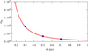 |
Fig. A.1 Conversion from distance to the star, d*, to G0 at the cloud edge. |
A.2 d to AV
Figure A.2 shows the conversion from AV to physical size for different radiation fields. The equation linking AV to d is
![Mathematical equation: $\[d=\frac{N_{\mathrm{H}}}{E_{\mathrm{B}-\mathrm{V}}} \frac{1}{R_{\mathrm{V}}} \int \frac{d A_{\mathrm{V}}}{n_{\mathrm{H}}\left(A_{\mathrm{V}}\right)},\]$](/articles/aa/full_html/2026/01/aa57445-25/aa57445-25-eq27.png) (A.1)
(A.1)
where ![Mathematical equation: $\[\frac{N_{\mathrm{H}}}{E_{\mathrm{B}-\mathrm{V}}}\]$](/articles/aa/full_html/2026/01/aa57445-25/aa57445-25-eq28.png) and RV are given in Table 1.
and RV are given in Table 1.
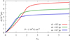 |
Fig. A.2 The conversion from AV to the spatial size, d. |
A.3 AV to NH
It follows directly from the values in Table 1:
![Mathematical equation: $\[N_{\mathrm{H}}=\frac{N_{\mathrm{H}}}{E_{\mathrm{B}-\mathrm{V}}} \frac{1}{R_{\mathrm{V}}} A_{\mathrm{V}}=2.855 \times 10^{21} A_{\mathrm{V}} \mathrm{~cm}^{-2}.\]$](/articles/aa/full_html/2026/01/aa57445-25/aa57445-25-eq29.png) (A.2)
(A.2)
Appendix B HD molecular properties
We summarize here further molecular properties of HD that are relevant to our study.
B.1 Photodissociation
The photodissociation mechanism of interstellar HD is very similar to H2: absorption from a low lying rovibrational level of X to an upper electronic excited state is followed by a radiative decay toward the continuum of the X ground electronic state. Hence, for a transition from level ”l” (low) in the ground electronic state X to level ”u”, belonging to the upper electronic state, the efficiency of dissociation depends on four physical quantities:
The mean radiation field intensity over the line profile
![Mathematical equation: $\[\bar{J}_{u l}= \frac{1}{4 \pi} \int I_{u l} ~d \Omega\]$](/articles/aa/full_html/2026/01/aa57445-25/aa57445-25-eq30.png) (where Iul is the specific intensity of the line (in erg cm−2 s−1 sr−1 Å−1)) at the transition wavelength. This is a function of both the external radiation field intensity and the absorption probability along the line of sight by HD itself (self-shielding) and by other species, mainly ultraviolet lines of H2 and continuum absorption by grains and ionization of light atoms (C and S). That quantity is obtained from the resolution of the radiative transfer equation as described in Le Petit et al. (2006).
(where Iul is the specific intensity of the line (in erg cm−2 s−1 sr−1 Å−1)) at the transition wavelength. This is a function of both the external radiation field intensity and the absorption probability along the line of sight by HD itself (self-shielding) and by other species, mainly ultraviolet lines of H2 and continuum absorption by grains and ionization of light atoms (C and S). That quantity is obtained from the resolution of the radiative transfer equation as described in Le Petit et al. (2006).The population nl of HD levels at the position of absorption is obtained from the solution to the detailed balance equations 1. It is important to realize that they may depend on the whole structure of the cloud due to the radiative induced terms.
-
The absorption probability that involves the Blu Einstein coefficient is related to the spontaneous emission coefficient Aul through a relation which depends on the units used for the radiation field. For the incident intensity J expressed in erg s−1 cm−2 Å−1 sr−1; this is
![Mathematical equation: $\[B_{l u}=10^{32} \frac{g_u}{g_l} \frac{\lambda^5}{2 ~h ~c^2} A_{u l},\]$](/articles/aa/full_html/2026/01/aa57445-25/aa57445-25-eq31.png) (B.1)
(B.1)where λ is expressed in Å.
The dissociation probability
![Mathematical equation: $\[p_{u}^{d i s}\]$](/articles/aa/full_html/2026/01/aa57445-25/aa57445-25-eq32.png) , i.e., the fraction of radiative transitions emitted above the dissociation limit of the
, i.e., the fraction of radiative transitions emitted above the dissociation limit of the ![Mathematical equation: $\[X { }^{1} \Sigma_{g}^{+}\]$](/articles/aa/full_html/2026/01/aa57445-25/aa57445-25-eq33.png) electronic ground state of HD, that is a property of the upper rovibronic level of the predissociative transition.
electronic ground state of HD, that is a property of the upper rovibronic level of the predissociative transition.
Then, the dissociation rate, expressed in cm−3 s−1, involving a transition l − u, at a specific wavelength λ, is given by
![Mathematical equation: $\[k_l=n_l \sum_u \bar{J}_{u l} ~B_{l u} ~p_u^{d i s}=n_l ~D_l.\]$](/articles/aa/full_html/2026/01/aa57445-25/aa57445-25-eq34.png) (B.2)
(B.2)
The product ![Mathematical equation: $\[B_{l u} \times p_{u}^{d i s}\]$](/articles/aa/full_html/2026/01/aa57445-25/aa57445-25-eq35.png) , or alternatively11
, or alternatively11 ![Mathematical equation: $\[A_{u l} \times p_{u}^{d i s}\]$](/articles/aa/full_html/2026/01/aa57445-25/aa57445-25-eq36.png) , (hereafter the “dissociation efficiency factor”) is an intrinsic property of the molecule, and can be evaluated before hand. Fig. B.1 shows this parameter for the strongest dissociating lines starting from X, v = 0, J = 2, which is significantly populated in zone I (see Figure 6), and toward levels of B (Lyman system). Aul decreases with v′ (upper level vibrational quantum number), in compliance with the Franck-Condon principle, but
, (hereafter the “dissociation efficiency factor”) is an intrinsic property of the molecule, and can be evaluated before hand. Fig. B.1 shows this parameter for the strongest dissociating lines starting from X, v = 0, J = 2, which is significantly populated in zone I (see Figure 6), and toward levels of B (Lyman system). Aul decreases with v′ (upper level vibrational quantum number), in compliance with the Franck-Condon principle, but ![Mathematical equation: $\[p_{u}^{d i s}\]$](/articles/aa/full_html/2026/01/aa57445-25/aa57445-25-eq37.png) is negligible for small v′ values and increases sharply with v′. As a result, the most efficient dissociating lines in the Lyman band system are P and R transitions involving v′ ~ 8–20.
is negligible for small v′ values and increases sharply with v′. As a result, the most efficient dissociating lines in the Lyman band system are P and R transitions involving v′ ~ 8–20.
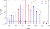 |
Fig. B.1 Dissociation efficiency factor of HD lines for transitions starting from v = 0, J = 2. Vertical bars are for the P and R lines. The attached number is v′. |
B.2 D + H2 → H + HD and HD + H → H + HD
The title reactions involving the major neutral hydrogen and deuterium species have a barrier of respectively E2 = 3820 K and E5 = 4240 K. Their contribution to formation and destruction of HD depends on whether sufficient energy in the molecular reactant is available to overcome this barrier. Bossion et al. (2019) and Bossion et al. (2020) have studied these two reactions which lead to the formation and destruction contributions shown in Fig. 5 in Sect. 3.4 in a state-to-state quasi-classical trajectory approach.
We tested these results against two other procedures that are found in the literature, in the absence of such a knowledge, when the reaction rate coefficient is given by an Arrhenius-type formula:
![Mathematical equation: $\[k_i=\alpha_i\left(\frac{T}{300}\right)^{\beta_i} \exp \left(-\frac{E_i}{T}\right).\]$](/articles/aa/full_html/2026/01/aa57445-25/aa57445-25-eq38.png) (B.3)
(B.3)
- (1)
No internal energy is available in the molecular reactant and only the kinetic form of energy (thermal) allows the reaction to occur. This is the approximation usually found in chemical models, where reaction rate coefficients are computed using the previous equation. The values of αi and βi are found in chemical kinetics databases such as KIDA and UMIST12. Gay et al. (2011) give analytic expressions of the reaction rate coefficients of both D + H2 → HD + H and HD + H → H2 + D reactions as 7.5 × 10⁻¹¹ exp(−3820/T) and 7.5 × 10⁻¹¹ exp(−4240/T) respectively. These reactions are thus important mainly in the warm front region of the PDR.
- (2)
Including internal excitation of the molecular reactant as introduced by Agúndez et al. (2010) for the C+ + H2 → CH+ + H endothermic reaction. Each reactive collision occurs with a H2 molecule in a (v, J) level of internal energy Ev, J. This energy is used to overcome the barrier, and the reaction rate is assumed to be
![Mathematical equation: $\[k_i=\alpha_i\left(\frac{T}{300}\right)^{\beta_i} \sum_{v, J} x_{v, J} ~\exp \left(-\frac{\max \left(0, E_i-E_{v, J}\right)}{T}\right),\]$](/articles/aa/full_html/2026/01/aa57445-25/aa57445-25-eq39.png) (B.4)
(B.4)where xv,J is the relative abundance of level (v, J). If Ev,J > Ei, the reaction rate coefficient becomes
![Mathematical equation: $\[k_{i}= \alpha_{i}\left(\frac{T}{300}\right)^{\beta_{i}} {\sum}_{v, J} ~x_{v, J}\]$](/articles/aa/full_html/2026/01/aa57445-25/aa57445-25-eq40.png) .
.
Figure B.2 shows the modifications to HD formation and destruction under these two hypotheses as compared to Fig. 5b. Fig. B.3 shows the fractional abundance of HD (panel (a)) and the total abundance of one selected vibrational level (panel (b), v = 1, J = 2) for the three possible rate coefficients considered here. Panel (a) shows that internal energy allows HD to form efficiently closer to the edge of the cloud, thanks to the efficiency of reactions with excited H2. As a consequence, vibrationally excited levels are more abundant, which leads to higher vibrational lines intensities.
We notice that the detailed picture of state-to-state reactivity leads to a significant increase of computing time. However, the importance of accounting for internal energy of reactants and products13 is recognized in various astrochemical studies (Goicoechea & Roncero 2022) but very few detailed results are available up to now.
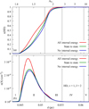 |
Fig. B.3 Comparison of HD abundance considering the different hypothesis (state-to-state, case (1) and case (2)). (a) Deuterium molecular fraction as a function of distance from the ionization front, d. The red line is for case (2), all internal energy used, the green line is for the state-to-state chemistry, and blue is for case (1) analytic expressions from Gay et al. (2011) using no internal energy. (b) Abundance of level v = 1 and J = 2. |
Appendix C Chemical heating
Chemical heating is hard to evaluate in a low density medium where collisional equilibrium does not dominate and thermal equilibrium is not achieved. Ideally, one should use the full state dependent cross-sections for both reactants and products, and sum over their energy distribution to compute the balance of the mean kinetic energy. This is clearly impossible in the present case, and one has to resort to cruder approximations. The exchange of chemical energy is expressed as the product of the enthalpy variation involved in the reaction by the number of reactions per unit time and per unit space (i.e., the reaction rate coefficient used to solve the chemical composition of the gas, which is already known), that is n(A) n(B) kAB ΔH in cm cm s−3 erg−1 for a binary reaction A + B → C + D + ΔH (Atkins et al. 2009)
kAB includes any impact of a possible barrier. ΔH is an intrinsic property of the reaction. From standard text books on thermochemistry (see, e.g., Atkins et al. (2009)), it is equal to the thermal energy given to or removed from the gas at constant pressure, including all internal excitation effects, for a medium connected to a heat reservoir. This is not exactly the case in a low density medium because other physical processes, such as spontaneous radiative transitions, modify the internal distribution of energy of the molecules. However, we have no way to evaluate their possible impact.
The main input energy is provided by the external incident radiation field and the cosmic ray particles. We do not consider possible mechanical energy due to shocks nor other contributions due to the presence of a magnetic field. Cosmic rays dominate deep into the cloud, but ultraviolet photons are the main source of energy in the outer shells. This radiative energy may be converted into internal or kinetic energy through different coupling mechanisms. Photoelectric effect on grains is very efficient to convert radiative energy into gas heating but gas-phase processes can also take place for such a conversion of energy, as illustrated in Fig. C.1.
 |
Fig. C.1 Energy transfer from the ultraviolet external bath to internal heating of the gas by chemistry. |
- (1)
First, external UV photons energy is transferred to H2 vibrational levels by absorption followed by cascades, with a 90% probability. As vibrational levels of H2 are located above 6000 K (corresponding to v = 1) above the fundamental level, they may provide a significant energy reservoir if they become populated.
- (2)
A part of the internal energy of H2, excited by UV pumping, is then transferred to chemical potential energy through the C+ + H2 reaction. This endothermic formation reaction of CH+requires some energy input to proceed. The internal energy of H2 has been first suggested by Stecher & Williams (1974) for explaining the presence of ubiquitous CH+in diffuse environments. This suggestion has been further quantified and established (Hierl et al. 1997; Agúndez et al. 2010; Naylor et al. 2010; Godard & Cernicharo 2013; Nagy et al. 2013). In the present model, we use a combination of Zanchet et al. (2013) and Herráez-Aguilar et al. (2014) theoretical computations to build temperature and H2 (v, J) state dependent rate coefficients for this reaction.
- (3)
CH+ then reacts with H2, through exothermic reactions to form
![Mathematical equation: $\[\mathrm{CH}_{2}^{+}\]$](/articles/aa/full_html/2026/01/aa57445-25/aa57445-25-eq41.png) and
and ![Mathematical equation: $\[\mathrm{CH}_{3}^{+}\]$](/articles/aa/full_html/2026/01/aa57445-25/aa57445-25-eq42.png) .
. - (4)
These ions finally recombine with electrons through exothermic reactions, releasing as much as a few eV in the gas.
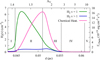 |
Fig. C.2 Comparison of the chemical heating contribution to H2 level abundance. Left axis: Abundance of vibrationally excited H2 as a function of distance from the ionization front, d, in the fiducial model. Right axis: Chemical heating contribution. |
Figure C.2 shows the abundance of vibrationally excited H2 and the contribution of chemistry to gas heating, as computed from the fiducial model. The later maximum is shifted toward the interior of the cloud because radiative and collisional deexcitation are more efficient than chemistry close to the edge of cloud. The process ceases where no vibrationally excited H2 remains.
Appendix D Uncertainties and error bars
D.1 Extinction curve induced uncertainties
The uncertainty on the extinction curve can be written as an uncertainty on RV and AV. If we consider that RV can be in the range RV = 3.1–5.5 (from a diffuse medium to a medium with a depletion of nanograins) and AV = 3.4 ± 1.0 in DF3. To maximize the uncertainty, we consider that the highest extinction possible is when considering an extinction curve with RV = 5.5 with AV = 4.4 and the lowest extinction possible when considering an extinction curve with RV = 3.1 with AV = 2.4. Then, the relative uncertainty on the line ratio due to the choice of the slope of the extinction curve can be written as
![Mathematical equation: $\[\begin{aligned}{\frac{d\left(I_1 / I_2\right)}{I_1 / I_2}}_{\text {extinction }}=\qquad\qquad\qquad\qquad\qquad\qquad\qquad\qquad\qquad\quad \\\frac{e^{-\frac{A_{\mathrm{V}}+d A_{\mathrm{V}}}{2.5 ~\log (e)}\left(\frac{A_{\lambda_1}}{A_{\mathrm{V}}}-\frac{A_{\lambda_2}}{A_{\mathrm{V}}}\right)\left(R_{\mathrm{V}}=5.5\right)}-e^{-\frac{A_{\mathrm{V}}-d A_{\mathrm{V}}}{2.5 ~\log (e)}\left(\frac{A_{\lambda_1}}{A_{\mathrm{V}}}-\frac{A_{\lambda_2}}{A_{\mathrm{V}}}\right)\left(R_{\mathrm{V}}=3.1\right)}}{e^{-\frac{A_{\mathrm{V}}}{2.5 ~\log (e)}\left(\frac{A_{\lambda_1}}{A_{\mathrm{V}}}-\frac{A_{\lambda_2}}{A_{\mathrm{V}}}\right)\left(R_{\mathrm{V}}=5.5\right)}}.\end{aligned}\]$](/articles/aa/full_html/2026/01/aa57445-25/aa57445-25-eq43.png) (D.1)
(D.1)
The excitation temperature is
![Mathematical equation: $\[T_{\mathrm{ex}}=\frac{E_2-E_1}{k_{\mathrm{B}}} / ~\ln~ \left(\frac{N_1 g_2}{N_2 g_1}\right).\]$](/articles/aa/full_html/2026/01/aa57445-25/aa57445-25-eq44.png) (D.2)
(D.2)
Hence, the relative uncertainty on the temperature is
![Mathematical equation: $\[\frac{d T}{T}_{\text {extinction }}==\frac{k_B T}{E_2-E_1} \frac{d\left(I_1 / I_2\right)}{I_1 / I_2}_ \text { extinction }\]$](/articles/aa/full_html/2026/01/aa57445-25/aa57445-25-eq45.png) (D.3)
(D.3)
Using the 1-0 P(1) (λ1 = 2.82 μm, E1 = 5225 K) and 1-0 R (3) line (λ1 = 2.53 μm, E2 = 6441 K) and AV ~ 3, we derive ![Mathematical equation: $\[\frac{d\left(I_{1} / I_{2}\right)}{I_{1} / I_{2}} \sim 0.06\]$](/articles/aa/full_html/2026/01/aa57445-25/aa57445-25-eq46.png) . In DF3, Tex = 484 K, thus
. In DF3, Tex = 484 K, thus ![Mathematical equation: $\[\frac{d T}{T}{ }_{\text {extinction}} \sim 0.03\]$](/articles/aa/full_html/2026/01/aa57445-25/aa57445-25-eq47.png) .
.
D.2 Error bars on mean values and fit parameters
If two lines are detected coming from the same upper level, the derived column densities are combined to reduce the uncertainties. Each measurement is issued from independent distributions with the same mean. Hence we can combine them under a maximum likelyhood hypothesis. Given two measures (N1, σ1) and (N2, σ2), the mean and uncertainty are given by:
![Mathematical equation: $\[N_J=\frac{\frac{N_1}{\sigma_1^2}+\frac{N_2}{\sigma_2^2}}{\frac{1}{\sigma_1^2}+\frac{1}{\sigma_2^2}}; \quad \sigma_J=\sqrt{\frac{1}{\frac{1}{\sigma_1^2}+\frac{1}{\sigma_2^2}}}\]$](/articles/aa/full_html/2026/01/aa57445-25/aa57445-25-eq48.png) (D.4)
(D.4)
Excitation temperatures obtain from linear fit on the quantities ![Mathematical equation: $\[y_{J}=\ln \frac{N_{J}}{g_{J}}\]$](/articles/aa/full_html/2026/01/aa57445-25/aa57445-25-eq49.png) . Given an uncertainty σJ on NJ, the uncertainty on yJ is
. Given an uncertainty σJ on NJ, the uncertainty on yJ is ![Mathematical equation: $\[\frac{\sigma_{J}}{N_{J}}\]$](/articles/aa/full_html/2026/01/aa57445-25/aa57445-25-eq50.png) . Note that the factor gJ simplifies from the ratio.
. Note that the factor gJ simplifies from the ratio.
Appendix E Line intensities
In this Appendix, we give a list of HD line intensities for the fiducial model P = 5 × 10⁷ Kcm−3 and d* = 0.5 pc. The choice of lines is limited to ITh > 10−7 erg cm−2 s−1 sr−1. We note that Joblin et al. (2018) report a value of 11 ± 4 × 10⁻⁵ erg cm−2 s−1 sr−1 for the pure rotational R(1) line, detected with Herschel, within a factor of 2 from our results. All Q lines and quadrupolar transitions are below this threshold. Most of these lines are too weak to be seen with today’s observing facilities, but the full set may be of interest for comparison purposes.
Line intensities of v = 0 → v = 0 transitions.
Line intensities of v = 1 → v = 0 transitions.
Line intensities of v = 2 → v = 1 transitions.
Line intensities of v = 3 → v = 2 transitions.
Line intensities of v = 2 → v = 0 transitions.
Line intensities of v = 3 → v = 0 transitions.
Line intensities of v = 3 → v = 0 transitions.
All Tables
Integrated intensities and upper level column densities of HD observed rovibrational lines in DF2 and DF3.
All Figures
|
Fig. 1 JWST NIRCam composite image of the Orion Bar, located in the Orion molecular cloud (Habart et al. 2024). Red shows the 3.35 μm emission (F335M filter), blue highlights the emission of Paα (F187N filter subtracted by F182M filter), and green indicates the emission of the H2 0–0 S(9) line at 4.70 μm (F470N filter subtracted by F480M filter). The white box represents the field of view of NIRSpec. The blue boxes correspond to the aperture where the spectra are averaged in the three dissociation fronts (DF1, DF2 and DF3). |
| In the text | |
|
Fig. 2 Variations of temperature, density and abundances as a function of distance from the ionization front, d, and visual extinction, AV, for the fiducial model. See Sect. 3.2 for the definitions of zones I to V. (a) Temperature (red line, left axis) and density profiles (blue line, right axis). (b) Relative abundances of H and H2, (resp. D and HD), normalized by n(H) + n(H2) (resp. n(D) + n(HD)). Values at the transitions are given in Table 2. |
| In the text | |
|
Fig. 3 Main contributions to (a) heating (Γ) and (b) cooling (Λ) of the gas as a function of distance d from the ionization front and visual extinction, AV. Each heating (resp. cooling) term is normalized by the total heating/cooling. |
| In the text | |
|
Fig. 4 Radiative energy density uλ at AV ~ 1.7 (d = 0.05 pc) in the 96–96.3 nm far ultraviolet wavelength range. Blue indicated H2 lines, while red shows HD lines. The positions of three strong HD absorption lines are shown using black vertical lines, coming from v = 0, J = 1 and J = 2. |
| In the text | |
|
Fig. 5 Relative contribution of HD formation and destruction reactions normalized to the total formation rate. (a): Individual reactions (2)–(9). (b) Sum of direct and reverse reactions. The y-axis is dimensionless. |
| In the text | |
|
Fig. 6 Hydrogen deuteride excited rotational levels abundance profiles as a function of distance from the ionization front, d, and visual extinction, AV. (a) v = 0 (top panel), (b) v = 1, (c) v = 2. See Fig. C.2 for a comparison with H2. |
| In the text | |
|
Fig. 7 Full modeled excitation diagram for HD. Light blue lines indicates fits to lowest J for each v giving the indicated excitation temperatures Tex, light golden lines shows fits to high J giving a |
| In the text | |
|
Fig. 8 Excitation balance |
| In the text | |
|
Fig. 9 NIRSpec continuum-subtracted observed spectrum. The dashed vertical red lines are the position of the first rovibrational v = 1 → 0 HD lines. From top to bottom, this figure shows the spectrum of the dissociation fronts of the Orion Bar: DF1, DF2, DF3. The apertures taken to average these spectra are from Peeters et al. (2024) for the dissociation fronts. These spectra are not corrected for extinction. |
| In the text | |
|
Fig. 10 Normalized integrated intensity profiles of the HD 1–0 R(0) line, H2 0–0 S(1) line, and H2 1–0 S(1) line across the third dissociation front DF 3 as a function of the projected distance to the star Θ1 Ori C. The distance to the Orion Bar used to calculate the distance to the star in arcsec is d = 414 pc (Menten et al. 2007). Each point corresponds to the intensity averaged on apertures with width of 2.5″ and height of 0.4″ with an angle of 38° (to match DF3 orientation) to increase the S/N. |
| In the text | |
|
Fig. 11 Excitation diagram of HD rovibrational lines in the DF3 (a) and the DF2 (b). The arrows correspond to the upper limits of HD lines which cannot be properly measured. The solid lines correspond to the fit to the distribution. The y-axis scales are identical to allow a visual comparison of Tex. |
| In the text | |
|
Fig. 12 Comparison of observational (red) and theoretical (blue) spectra. The vertical dash-dotted lines indicate lines of H2. The vertical cyan and pink lines indicate recombination lines of H and He respectively. The vertical green lines show the location of HD transitions. The theoretical spectrum is computed for an angle of view of 70°. |
| In the text | |
|
Fig. 13 Comparison of observational (in red) and theoretical (in green) excitation diagrams for v = 1. Theoretical column densities have been computed for an angle of view of 70°. |
| In the text | |
|
Fig. 14 Size of zone I for PDR models at different thermal pressure and UV field intensity (scaled by the distance to the star). |
| In the text | |
|
Fig. 15 Excitation temperature for v = 1 for various values of P and d*. The observational range of excitation temperatures is displayed as a colored band: yellow for DF3 and purple for DF2. |
| In the text | |
|
Fig. A.1 Conversion from distance to the star, d*, to G0 at the cloud edge. |
| In the text | |
|
Fig. A.2 The conversion from AV to the spatial size, d. |
| In the text | |
|
Fig. B.1 Dissociation efficiency factor of HD lines for transitions starting from v = 0, J = 2. Vertical bars are for the P and R lines. The attached number is v′. |
| In the text | |
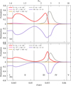 |
Fig. B.2 Same as Fig. 5b but for (a) case (1) and (b) case (2). |
| In the text | |
|
Fig. B.3 Comparison of HD abundance considering the different hypothesis (state-to-state, case (1) and case (2)). (a) Deuterium molecular fraction as a function of distance from the ionization front, d. The red line is for case (2), all internal energy used, the green line is for the state-to-state chemistry, and blue is for case (1) analytic expressions from Gay et al. (2011) using no internal energy. (b) Abundance of level v = 1 and J = 2. |
| In the text | |
|
Fig. C.1 Energy transfer from the ultraviolet external bath to internal heating of the gas by chemistry. |
| In the text | |
|
Fig. C.2 Comparison of the chemical heating contribution to H2 level abundance. Left axis: Abundance of vibrationally excited H2 as a function of distance from the ionization front, d, in the fiducial model. Right axis: Chemical heating contribution. |
| In the text | |
Current usage metrics show cumulative count of Article Views (full-text article views including HTML views, PDF and ePub downloads, according to the available data) and Abstracts Views on Vision4Press platform.
Data correspond to usage on the plateform after 2015. The current usage metrics is available 48-96 hours after online publication and is updated daily on week days.
Initial download of the metrics may take a while.