| Issue |
A&A
Volume 705, January 2026
|
|
|---|---|---|
| Article Number | A235 | |
| Number of page(s) | 9 | |
| Section | Galactic structure, stellar clusters and populations | |
| DOI | https://doi.org/10.1051/0004-6361/202557723 | |
| Published online | 27 January 2026 | |
Chemical analysis of the Milky Way’s nuclear star cluster
Evidence for a metallicity gradient
1
Université Côte d’Azur, Observatoire de la Côte d’Azur, Laboratoire Lagrange, CNRS,
Blvd de l’Observatoire,
06304
Nice,
France
2
MAUCA – Master track in Astrophysics, Université Côte d’Azur, Observatoire de la Côte d’Azur,
Parc Valrose,
06100
Nice,
France
3
Instituto de Astrofísica de Andalucía (CSIC),
Glorieta de la Astronomía s/n,
18008
Granada,
Spain
4
Department of Astrophysics, University of Vienna,
Türkenschanzstrasse 17,
1180
Wien,
Austria
5
Aryabhatta Research Institute of Observational Sciences,
Manora Peak,
Nainital
263002,
India
6
Como Lake centre for AstroPhysics (CLAP), DiSAT, Università dell’Insubria,
Via Valleggio 11,
22100
Como,
Italy
7
Institute of Space Sciences & Astronomy, University of Malta,
Msida MSD 2080,
Malta
8
Division of Astrophysics, Department of Physics, Lund University,
Box 118,
22100
Lund,
Sweden
★ Corresponding author: This email address is being protected from spambots. You need JavaScript enabled to view it.
Received:
16
October
2025
Accepted:
6
December
2025
Abstract
Context. The Milky Way nuclear star cluster (MWNSC) is located in the Galactic centre, together with the Milky Way nuclear stellar disc (MWNSD), and they dominate the gravitational potential within the inner 300 pc. However, the formation and evolution of the two systems and their possible connections are still under debate.
Aims. We reanalysed the low-resolution KMOS spectra in the MWNSC with the aim of improving the stellar parameters (Teff, log g, and [M/H]) for the MWNSC.
Methods. We used an improved line list, especially dedicated for cool M giants, that allowed us to improve the stellar parameters and to obtain in addition global α-elements. A comparison with high-resolution IR spectra (from IGRINS) gives very satisfactory results and constrains the uncertainties to Teff ≃ 150 K, log g ≃ 0.4 dex, and [M/H] ≃ 0.2 dex. Our α-elements agree within 0.1 dex compared to the IGRINS spectra.
Results. We obtained a high-quality sample of 1140 M giant stars where we see an important contribution of a metal-poor population (∼20%) centred at [M/H] ≃−0.7 dex, while the most dominant part comes from the metal-rich population with [M/H] ≃ 0.26 dex. We constructed a metallicity map and find a metallicity gradient of ∼−0.1 ± 0.02 dex/pc favouring the inside-out formation scenario for the MWNSC.
Key words: stars: abundances / stars: late-type / Galaxy: abundances / Galaxy: center / Galaxy: nucleus / Galaxy: stellar content
© The Authors 2026
 Open Access article, published by EDP Sciences, under the terms of the Creative Commons Attribution License (https://creativecommons.org/licenses/by/4.0), which permits unrestricted use, distribution, and reproduction in any medium, provided the original work is properly cited.
This article is published in open access under the Subscribe to Open model. This email address is being protected from spambots. You need JavaScript enabled to view it. to support open access publication.
1 Introduction
Nuclear star clusters (NSCs) are compact and massive clusters located at the dynamical centres of their host galaxies. Their effective radii, within which half of the cluster light is contained, are found to span a wide range from 0.4 to 44 pc (Neumayer et al. 2020). The two proposed formation mechanisms are, first, the inspiral and mergers of massive star clusters (e.g. Antonini et al. 2012; Hartmann et al. 2011) and, second, in situ formation (e.g. Aharon & Perets 2015; Brown et al. 2018). However, both scenarios could possibly contribute to the growth of NSCs (Böker 2010). Moreover, the in situ formation can be caused by several secular mechanisms such as bar-driven gas infall (Shlosman et al. 1990), dissipative nucleation (Bekki et al. 2006; Bekki 2007), tidal compression (Emsellem & van de Ven 2008) or magneto-rotational instability (Milosavljević 2004). Fahrion et al. (2021) argued that there appears to be a distinction of the formation mechanism with galaxy mass, where less massive NSCs are produced mainly by cluster infall, while more massive NSCs are formed in situ with a transition galaxy mass of about ∼109 M⊙.
The Milky Way also features a NSC (hereafter called MWNSC) in its centre with an effective radius between 4.2 ± 0.4 pc and 7.2 ± 2.0 pc (Schödel et al. 2014a; Fritz et al. 2016; Gallego-Cano et al. 2020). The mass of the MWNSC is between 2.1 ± 0.7 × 10⁷ and 4.2 ± 1.1 × 10⁷ M⊙ (Schödel et al. 2014a, 2020; Chatzopoulos et al. 2015; Feldmeier et al. 2014; Feldmeier-Krause et al. 2017b).
The MWNSC is embedded inside the Milky Way nuclear stellar disc (MWNSD), which is a central, kinematically cold, distinct, rotating structure (v/σ ≃ 1, Schultheis et al. 2025). The MWNSD can be described by an exponential intensity radial profile and is thought to be formed from gas brought to the centre by the bar via the central molecular zone (see e.g. Sormani et al. 2024). The radial and vertical scale lengths for the MWNSD are  and
and  , respectively (Gallego-Cano et al. 2020; Sormani et al. 2022), and the total mass is
  (Sormani et al. 2022).
While several photometric studies suggest that the MWNSD and MWNSC may have undergone distinct formation histories (Nogueras-Lara et al. 2020, 2021b), Nogueras-Lara et al. (2023) found kinematic and metallicity gradients that suggest a smooth transition between the two components. They propose that the MWNSD and MWNSC might be part of the same structure. In addition, Seth et al. (2006) found discs or rings superimposed onto the observed NSCs in the nuclear regions of 14 nearby galaxies. They suggest that their observations may support an in situ formation where NSCs are formed from stars losing angular momentum from the NSDs in which the NSCs are embedded. However, the links between NSDs and NSCs are still under debate (see also Schultheis et al. 2025).
Due to the extreme extinction towards the MWNSC (Av ∼30), only observations in the infrared are possible (Schödel et al. 2010; Nogueras-Lara et al. 2018). Even spectroscopic surveys such as APOGEE could only observe a few very luminous stars in the NSC, due to its limiting sensitivity (Schultheis et al. 2020). Feldmeier-Krause et al. (2017a) and Feldmeier-Krause et al. (2020) used an extensive dataset of K-band Multi Object Spectrograph (KMOS) data (ESO/VLT) to perform a chemical study (i.e. metallicities) of stars located in the MWNSC. They find a predominantly metal-rich population with a mean metallicity of 0.34 dex with some indications of an anisotropic metallicity distribution function, i.e. a higher fraction of subsolar metallicity stars in the Galactic north. They argue that this anisotropy could be due to star cluster infall events (see e.g. Antonini et al. 2012; Perets & Mastrobuono-Battisti 2014; Arca Sedda et al. 2020; Do et al. 2020). Feldmeier-Krause et al. (2025) conducted a first spectroscopic survey from the MWNSC to the inner MWNSD, out to ± 32 pc from Sgr A*. They provided a first global map of the mean metallicity and found a decrease in [M/H] towards the centre of the MWNSC. However, as discussed by the authors, this decrease in metallicity could be due to a projection effect.
One difficulty in all the above-mentioned studies is the fact that these spectra have low spectral resolution (R ∼3000−4000). The vast majority of the studied stellar populations are cool M giant stars with temperatures below 4000 K. The spectral analysis for these stars is extremely challenging, even for high-resolution spectra (see e.g. Thorsbro et al. 2023; Ryde et al. 2025; Nandakumar et al. 2025) where line blends with molecules is a big issue.
For this paper we reanalysed the KMOS dataset of Feldmeier-Krause et al. (2020), taking advantage of a recent improved line list, specifically adapted for cool M giants and that has been also used for high-resolution spectroscopic studies (Ryde et al. 2025). We used available high-resolution spectra of cool M giants covering a similar stellar parameter space to validate our method.
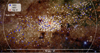 |
Fig. 1 GALACTICNUCLEUS JHKs false-colour image of the region covered by FK1720. The blue circles and white diamonds respectively mark stars classified as belonging to the MWNSD and MWNSC, according to the criterion described in Sect. 2.1. The white dashed line indicates the effective radius of the MWNSC, and the compass shows the Galactic coordinates. |
2 Data
We used the dataset of Feldmeier-Krause et al. (2017a) and Feldmeier-Krause et al. (2020) (hereafter FK1720) observed by KMOS (Sharples et al. 2013) at the VLT, which we have reanalysed. KMOS consists of 24 Integral Field Units (IFUs) with a field of view of 2.8′′ × 2.8′′ each. The spatial scale is 0.2′′/pix × 0.2′′/pix. The central field was observed twice by Feldmeier-Krause et al. (2017a) and centred on the MWNSC. We refer here to Feldmeier-Krause et al. (2017a) for more details of the dataset. Feldmeier-Krause et al. (2020) extended the central field by observing six mosaic fields within the half-light radius of the MWNSC (∼4−5 pc; Schödel et al. 2014b; Gallego-Cano et al. 2020). Figure 1 shows the target field and the observed stars.
The wavelength coverage of these spectra is in the range 19 340−24 600 Å with a spectral resolution of ∼2.8 Å pixel−1. As the spectral resolution of KMOS varies spatially, we used the resolution maps as well as the radial velocities from FK1720 as an input for the Bayesian STARKIT code (Kerzendorf & Do 2015). For a more detailed description of the dataset we refer to FK1720. Most of the stars have repeated observations, which we treat separately.
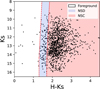 |
Fig. 2 H−K vs K colour-magnitude diagram of our data sample. Stars that are members of the MWNSC are indicated in red, stars that are members of the MWNSD are in blue, and the foreground objects are in white. For our work, here we only use stars in the MWNSC. |
2.1 MWNSC membership
To identify MWNSC stars and obtain a photometric counterpart for each target star, we cross-matched the FK1720 KMOS stellar sample with the HKs photometry from the GALACTICNUCLEUS survey (Nogueras-Lara et al. 2018, 2019). This catalogue provides state-of-the-art, high angular resolution (∼0.2′′), near-infrared photometry of the Galactic centre. To avoid saturation for GALACTICNUCLEUS sources with Ks ≲11.5, we complemented the data with the SIRIUS/IRSF catalogue (e.g. Nagayama et al. 2003; Nishiyama et al. 2006), replacing saturated stars with undetected ones as described in Nogueras-Lara et al. (2022).
We then used common stars to align the two catalogues, and adopted a maximum search radius of ∼0.3′′, corresponding to half the typical angular resolution of the KMOS data (e.g. Feldmeier-Krause et al. 2017a). This yielded ∼1300 stars with HKs photometry.
To separate the Galactic components, we applied a photometric criterion to distinguish between foreground stars (likely belonging to spiral arms along the line of sight and to the Galactic bulge; e.g. Nogueras-Lara et al. 2021a), MWNSD stars, and MWNSC stars, following the method described in Nogueras-Lara et al. (2023). This approach assumes a correlation between distance and extinction along the line of sight, which allows us to statistically differentiate these components by applying a colour cut, as shown in Fig. 2.
2.2 Data completeness
To estimate the completeness of the KMOS sample, we constructed a Ks luminosity function and compared it with a scaled reference function based on all GALACTICNUCLEUS stars detected in Ks within the target region. We then computed the completeness by assuming that the reference catalogue is approximately fully complete in the relevant region and magnitude range (e.g. Nogueras-Lara et al. 2020). Figure 3 shows the resulting completeness, indicating that the spectroscopic sample is ≳60% complete up to Ks=13.
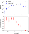 |
Fig. 3 Completeness of the KMOS FK1720 sample. Upper panel: Ks luminosity functions from the KMOS sample and the reference sample of GALACTICNUCLEUS (GNS) stars in the region. The associated uncertainty was estimated as the square root of the number of stars per magnitude bin. Lower panel: completeness function obtained by comparing the two Ks luminosity functions. |
2.3 Analysis
As in FK1720, we used the full spectral fitting code STARKIT (Kerzendorf & Do 2015), but added some specific improvements for the analysis of cool stars. STARKIT interpolates the template spectra and applies a Bayesian sampling (Multinest, Feroz & Hobson 2008) to obtain the best spectral fit using a grid of synthetic spectra. A key improvement in this work is the use of a dedicated synthetic model grid optimized for cool giants (see Sect. 2.4). By contrast, FK1720 based their analysis on the PHOENIX stellar library (Husser et al. 2013), which neither incorporates the updated line lists adopted here nor includes support for NLTE effects.
In addition, we performed for each of the spectra a continuum normalization using a sixth-order polynomial function and applying a two-sigma clipping. As we assume that all stars in our sample are M giants, we set a uniform prior in temperature (2800<Teff<4600 K) and in the surface gravity (−0.5< log g < 3), typical values for M giants. Contrary to FK1720, we did not use any photometric criteria to constrain log g, due to the large uncertainties in the photometric surface gravities. Our specific grid also allows the α-elements to be computed (see Sect. 4.1). Our dedicated synthetic model grid covers the following stellar parameter ranges: 2800<Teff<4600 K,−0.5< log g<3,−1.2<[M/H]<0.6, and −0.4<[α/Fe]<0.6.
Each observed spectrum was modelled using synthetic spectra from a Spectroscopy Made Easy (SME, Valenti & Piskunov 2012; Piskunov & Valenti 2017)-based grid, convolved to match the instrument resolution. The spectral grid spans stellar atmospheric parameters including effective temperature (Teff), surface gravity (log g), metallicity ([M/H]), and alpha-enhancement ([α/Fe]). The observational data were pre-processed to exclude regions contaminated by Brγ, NaI, CaI, and the CO molecular features, in a similar way to FK1720 (see Fig. 4). For this work, we also derived the α-abundances of our stars (see Sect. 2.4).
A Bayesian inference framework was applied using the MultiNest nested sampling algorithm to explore the posterior distribution of stellar parameters. The likelihood evaluation was based on a χ2 comparison between the observed and model spectra.
The posterior probability distributions for each stellar parameter were obtained using the MultiNest algorithm, which provides a statistically rigorous sampling of the multidimensional parameter space. The sampling yields posterior samples that encode both the likelihood χ2-based spectral fit and the imposed priors. For each parameter, we derived the 50th percentile (median) of the posterior distribution together with its standard deviation (the square root of the variance in the posterior). To complement the posterior statistics, we computed the reduced χ2 of the best-fit model, defined as
 where N is the number of spectral data points, p is the number of free parameters, fobs, i and fmod, i are the observed and model fluxes, and σi is the per-pixel uncertainty.
Special attention is given to cases where posterior distributions are truncated near the grid edges, particularly for Teff, log g, and [M/H], where synthetic spectra are not defined outside the grid limits. In such cases, we flag these spectra and do not consider them for further analysis.
The α-elements were obtained by running STARKIT a second time, fixing the stellar parameters Teff and log g, but using [M/H] and [α/Fe] as free parameters. As in the first step, we used all the posterior parameters to trace the uncertainties as well as the border flags. For our prior we assumed that the α-elements follow the Galactic prior, meaning that for subsolar metallicities, the α-elements are enhanced, while for above-solar metallicities, the α-elements are solar or subsolar.
Figure 4 shows a typical spectrum of an M giant; in this case it is starId 30001001 with Teff=3550 ± 90 K, log g=1.1 ± 0.18 dex,[M/H]=0.01 ± 0.15 dex, and [α/Fe]= −0.02 ± 0.11 dex.
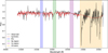 |
Fig. 4 Example of a spectral fit using STARKIT for starId 30001001. The normalized observed spectrum is in black; the best synthetic fit is indicated in red. The vertical bands show the masks applied: blue is the Brγ region, green the region around the NaI line, magenta the region around the CaI line, and orange the CO band heads. |
2.4 New model grid
To determine the stellar parameters – effective temperature (Teff), surface gravity (log g), and metallicity ([M/H]) – together with the α-element abundances of our targets, we generated a grid of synthetic spectra using the spectral synthesis code SME (Valenti & Piskunov 2012; Piskunov & Valenti 2017). SME interpolates on a grid of one-dimensional (1D) MARCS atmosphere models (Gustafsson et al. 2008), which are hydrostatic, spherically symmetric models computed under the assumptions of chemical equilibrium, homogeneity, and total flux conservation (radiative plus convective, with convective flux calculated via a mixing-length prescription).
In order to synthesize the spectra, an accurate list of atomic and molecular energy level transitions is required. In the list of atomic energy level transitions, we used the solar centre intensity atlas (Livingston & Wallace 1991) to update wavelengths and line strengths (astrophysical log g f-values) (Thorsbro et al. 2017; Nandakumar et al. 2024a). Since molecular lines are strong features in our spectra, the adopted line list includes relevant molecular transitions. For CN, the most dominant molecule apart from CO, whose lines dominate in the 2.3 μm bandhead region, we used the list of Sneden et al. (2014). The CO line data are from Li et al. (2015). At shorter wavelengths of our spectral region, SiO, H2O, and OH are important; their line lists are from Langhoff & Bauschlicher (1993), Polyansky et al. (2018), and Brooke et al. (2016), respectively.
The spectrum synthesis was carried out without assuming local thermodynamic equilibrium (LTE). Instead, we used precomputed grids of departure coefficients,  , where i denotes the level index for non-LTE (NLTE) and LTE populations n and n*, respectively. These coefficients were used to correct the LTE line opacities following the method described in Section 3 of Piskunov & Valenti (2017). For magnesium, silicon, and calcium, the grids of departure coefficients are those described in Amarsi et al. (2020), with model atoms from Osorio & Barklem (2016) and Osorio et al. (2019) for magnesium and calcium (fine structure collapsed) and from Amarsi & Asplund (2017) for silicon. For iron, we used the grid of departure coefficients and model atom presented in Amarsi et al. (2022).
The resulting SME model grid, spanning a range of Teff, log g, [M/H], and [α/Fe] values, was then used in the STARKIT framework (Kerzendorf & Do 2015; Do et al. 2015), which employs the MultiNest algorithm (Feroz & Hobson 2008) to perform a probabilistic grid search. STARKIT interpolates within the synthetic grid to find the model spectra that best match the observations, yielding posterior probability distributions for the stellar parameters and α-element abundances. This combined approach allowed us to systematically explore the parameter space, account for molecular and NLTE effects in our modelling, and derive robust values for Teff, log g,[Fe/H], and [α/Fe].
2.5 Quality control
Most of our sample has multiple exposures and we decided to keep only stars with Δ Teff<500 K, Δ log g<0.5 dex, and Δ[M/H]<0.3 dex. We only kept sources with a S/N>10 and rejected sources that are within 5% of the border grid of our grid of synthetic spectra. As pointed out by Feldmeier-Krause et al. (2017a), fringes can occur in the stellar spectra if the star is located at the edge of the IFU. As most of the stars had two or more exposures, we kept only those stars that fulfil the criteria mentioned above, and took the mean of the stellar parameters. In total, our sample consists of 1140 stars. As mentioned in Sect. 2.1, we excluded foreground stars and stars located in the NSD.
3 Validation with high-resolution spectra
We took advantage of the high-resolution high signal-to-noise sample of cool M giants in the solar neighbourhood from Nandakumar et al. (2024b), hereafter referred to as the SN comparison sample. These stars were observed with the Immersion GRating INfrared Spectrometer (IGRINS) spectrograph on the Gemini South telescope covering the full H- and K-bands with a spectral resolution of R=45 000. Their sample consists of 30 cool M giants with Teff ≤ 4000 K and a high signal-to-noise ratio (S/N>100) making it an ideal comparison sample to our KMOS stars. We convolved the high-resolution SN sample with a Gaussian kernel to the resolving power of KMOS (R=4000), assuming a constant R over the full wavelength range. We ran STARKIT over these degraded spectra using the same set-up as mentioned above (see Sect. 2.3).
In addition, seven M giants in our KMOS sample were observed with IGRINS and analysed in Nandakumar et al. (2025) and Ryde et al. (2025). These stars were observed with the same instrumental configuration as the SN sample and can be considered as benchmark stars in terms of stellar parameters and chemical abundances. We refer to this as the IGRINS/MWNSC sample; for a more detailed discussion about the analysis, we refer to Nandakumar et al. (2025).
Figure 5 shows the comparison of the stellar parameters (Teff, log g,[M/H],[α/Fe], from top to bottom). [M/H] is defined as the global metallicity: [M/H]=[Fe/H]+[α/Fe]. The black filled circles show the IGRINS SN sample and the red filled circles the corresponding IGRINS/MWNSC sample. In general, we see that the stellar parameters can be well recovered from the low-resolution spectra with nearly no systematic offsets. The typical uncertainties are ∼150 K in Teff, ∼0.4 dex in log g, ∼0.2 dex in [M/H], and ∼0.10 dex in [α/Fe]. We see a trend in the comparison with the global α-values, in the sense that the low-resolution spectra seem to overestimate the global α for high α-abundances. We performed a linear fit (last panel of Fig. 5), which gives us Δ[α/Fe]=0.5814 ×[α/Fe]−0.0233 and we applied this correction to our α-measurements. Nevertheless, Figure 5 clearly demonstrates that the stellar parameters can be reasonably well recovered from our KMOS sample.
4 Results
Figure 6 shows the comparison of the Kiel diagram with respect to FK1720 (left panel). We clearly see the improvement in the stellar parameters (Teff, log g, and [M/H]) covering the expected parameter space for typical red giant branch stars, which are also indicated by the PARSEC isochrones; the uncertainty for each of our stars is also indicated. The median uncertainties are of the order of Teff ≃ 150 K, log g ≃ 0.3 dex, and [M/H] ≃ 0.2 dex, and are even smaller when comparing the uncertainties with FK1720 (σTeff ≃ 212 K, σlog g ≃ 1 dex, σ[M/H] ≃ 0.26 dex). We also note that the highest metallicity in our grid is 0.6 dex and the coolest temperature is restricted to 2800 K. The grid of FK1720 spans a wider range with temperatures down to 2300 K and [M/H] up to 1 dex. The main reason for this improvement is related to the new grid of synthetic models together with imposing a uniform prior in Teff and log g. A slight improvement also comes in the continuum normalization. While FK1720 did the normalization within STARKIT using a fifth-order polynomial, we performed the continuum normalization before running STARKIT with a sixthdegree polynomial, and applied a sigma clipping (see Sect. 2.3) to remove outliers.
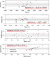 |
Fig. 5 Comparison between stellar parameters of high-resolution spectra to degraded spectra at the resolution of KMOS. The y-axis shows the difference between low-resolution and high-resolution spectra, respectively, while the x-axis displays the value from the low-resolution work. The shaded grey area shows ± 1 σ levels for each parameter comparison. The mean difference and standard deviations are indicated at the upper right. The black dots show the SN sample, while the red dots the NSC stars from Nandakumar et al. (2025). |
4.1 α-elements
The α-elements were obtained by running STARKIT a second time fixing the stellar parameters Teff and log g, but using [M/H] and α as free parameters. As in the first step, we used all the posterior parameters to trace the uncertainties as well as the border flags. For our prior we assumed that the α-elements follow the Galactic prior, meaning that for subsolar metallicities, the α-elements are in the range −0.2<[α/Fe]<0.4, while for super-solar metallicities, the α-elements are solar or subsolar (−0.2<[α/Fe]<0.2).
A running mean of [α/Fe], calculated with a dynamic window size (5% of the dataset or a minimum of ten stars), was applied to trace the underlying trend across metallicity. The error bars reflect the root mean square uncertainties of the averaged α-abundances. Figure 7 shows the expected α-enhancement at low metallicities, consistent with the enrichment by core-collapse supernovae at early times (Matteucci 2021). While the global α-trend can be seen as representative for the global chemical evolution trend, we note that the individual measurement uncertainties can be very large and should be treated with caution. This can also be seen in Fig. 5 where for high α-enhanced stars, the low-resolution spectra overestimate the α-abundances with respect to the high-resolution spectra.
 |
Fig. 6 Comparison of the Kiel diagram between FK1720 (left panel) and our work (right panel). Superimposed are the PARSEC stellar isochrones with an age of 8 Gyr and ranging in [M/H] from −1.2 dex (dark blue) to 0.6 dex (dark red). The standard deviations of Teff and log g is indicated for each star in grey. |
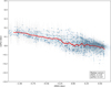 |
Fig. 7 [α/Fe] vs [M/H] diagram of 1171 stars. The standard deviations are indicated in grey, while the red line shows the running mean. |
4.2 Metallicity distribution function
We analysed the metallicity distribution function (MDF) of our sample by adapting a Gaussian mixture modelling (GMM) using the Bayesian information criterion (BIC) to determine the optimal number of components. The GMM parameters were refined using a Markov chain Monte Carlo (MCMC) sampler to account for metallicity measurement errors. Posterior distributions from the MCMC chains were used to compute median parameter values and their uncertainties. We generated 1000 random samples from the posterior to construct confidence intervals (68%, 95%, and 99%) for the total metallicity distribution, accounting for both model and measurement uncertainties. The GMM models favours a two-component model with a mean metallicity of −0.77 dex and a sigma of 0.24 dex for the metal-poor population and +0.26 dex with a sigma of 0.10 dex for the metal-rich population (see Fig. 8).
Our finding of a dominant metal-rich population is in agreement with FK1720. However, we find a more significant fraction of metal-poor stars (∼17% compared to 10% in FK1720) in the MWNSC. Nogueras-Lara (2022) showed that by using extinction values one can separate stars from the NSC and the NSD in the sense that stars in NSC show systematically higher interstellar reddening values (see Sect. 2.1). They concluded that the original FK1720 sample of stars shows a significant contribution of stars situated in the MWNSD. They obtain a larger fraction of metal-poor stars compared to FK1720, but their metallicity peaks at around −0.2 dex, which is much more metal-rich compared to our derived values (−0.76 dex). This difference is certainly due to our reanalysis of the FK1720 sample as we used the same selection criteria to remove stars from the MWNSD.
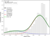 |
Fig. 8 Metallicity distribution function of our sample. A two-component GMM model is superposed. The first component is centred at −0.76 dex with a standard deviation of 0.24 dex, while the second component is centred at +0.26 dex with a std of 0.10 dex. The blue dashed lines represents the Gaussian fit for the metal-poor population, while the red dashed lines are for the metal-rich population. The total model is displayed with a solid black line together with the 3 σ uncertainties. |
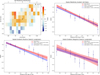 |
Fig. 9 (Upper left panel): mean metallicities in offset coordinates from Sgr A*. Galactic north is up. Each of the bins has at least five stars. (Upper right panel): mean metallicity as a function of the distance from Sgr A* (in pc). The error bars indicate the standard error of the mean metallicity within each bin (each bin has at least five stars). The blue dashed line shows the linear least-squares fit with the 95% confidence interval shown as the blue area. The red lines show the Bayesian MCMC analysis with the median prediction from the MCMC samples and the red area indicates the 16th–84th percentile uncertainty range from the MCMC posterior predictions. (Lower left panel): similar to the upper right panel, but only for positive Galactic longitudes. (Lower right panel): similar to upper right panel, but only for negative Galactic longitudes. |
4.3 Metallicity maps and gradients
As in FK1720, we trace the spatial distribution of the stars in our dataset as a function of metallicity to see any possible asymmetries. Figure 9, upper left panel, shows a metallicity map centred on Sgr A*. The bins are chosen to be 15′′ wide, which provides enough stars (>5 stars) in each metallicity bin.
The resulting metallicity map reveals a dominant very metal-rich population, but we also note a significant high fraction of subsolar metallicity towards the south. The upper right panel of Fig. 9 displays the mean metallicity as a function of the distance to Sgr A*, where we see a clear indication of a negative radial metallicity gradient with 0.1 ± 0.040 dex/pc. We tested the statistical significance of the metallicity gradient by applying a MCMC analysis using 32 walkers for 5000 steps following a 1000-step burn-in period. Our MCMC results are strongly consistent with the linear regression results with a slope of  with a highly significant p-value of 0.0002 (R2 ∼0.84) (see Fig. 9, upper right panel). This statistical analysis makes us confident of the reliability of our results showing a strong metallicity gradient within the MWNSC. The lower left and lower right panel shows the radial gradient for positive and negative Galactic longitudes, respectively, where we see some slight impact on the asymmetry at negative Galactic longitudes.
5 Discussions
Feldmeier-Krause (2022) studied the metallicity distribution of two fields along the Galactic plane, ∼20 pc east and west from Sgr A*, and found a continuous decrease in metallicity with increasing distance with respect to Sgr A*. Nogueras-Lara et al. (2023) analysed the transition region between the MWNSC and the MWNSD to better characterize the two structures. They use interstellar reddening as a proxy of the galactocentric distance and confirmed the metallicity gradient from Feldmeier-Krause (2022). Our derived metallicity maps and metallicity gradient of the NSC (see Fig. 9) are consistent with an inside-out formation scenario of the MWNSC.
The formation of the NSD in barred galaxies is mainly due to the bar-driven gas inflow to the centre of the galaxies (Schultheis et al. 2025). The gas inflow rates generate disc- or ring-like structures, such as the central molecular zone in the Milky Way (Morris & Serabyn 1996). The current idea is that star formation occurs in these gaseous rings, which build up nuclear stellar discs over time (Schultheis et al. 2025). While most of the gas is stalled at the nuclear ring, a small fraction can be transferred further to the NSC via nuclear inflows to the innermost few parsecs (see e.g. Moon et al. 2023; Tress et al. 2024), creating small circumnuclear rings. These circumnuclear rings can then grow with time leading to a metallicity gradient, typical for an inside-out formation scenario. The Milky Way hosts a small circumnuclear ring with a radius of 4 pc (Gallego-Cano et al. 2020), which is the typical size of the MWNSC.
Another way to connect the MWNSC and the MWNSD is if the MWNSD starts forming at the centre under the condition that the initial central mass concentration when the bar has formed is small (Schultheis et al. 2025). In that case the bar-driven inflow will drive gas directly to the centre forming the MWNSC and MWNSD at the same time where the MWNSC is the continuous inner part of the MWNSD. This scenario was suggested by Nogueras-Lara et al. (2023), who predicted the observed metallicity gradient and suggested that the MWNSC and MWNSD are essentially the same structure, where the MWNSD is the growing edge of the MWNSC.
For NSCs, several possible formation scenarios for in situ formation have been proposed, such as bar-driven gas infall, dissipative nucleation, tidal compression, or magneto-rotational instability (see Neumayer et al. 2020 for more details). The presence of a young stellar population concentrated at small radii (e.g. <0.5 pc in the Milky Way, Feldmeier-Krause et al. 2015) favours the scenario of an in situ formation of the NSC, which has been also detected in other NSCs such as M31 (Carson et al. 2015).
In our work, we established within the MWNSC a negative metallicity gradient, a clear signature of an inside-out formation, in a similar way to the MWNSD. The metal-poor stars are mainly located in the southern outer parts of the MWNSC, contrary to Feldmeier-Krause et al. (2020) where they found an anisotropy of low-metallicity stars in the Galactic north. While our fraction of metal-rich stars ([M/H]>0.3 dex) is 0.64 and is similar to that of Feldmeier-Krause et al. (2020), we get a much higher fraction of metal-poor stars (17% compared to 6% in FK20). We believe that our improved synthetic grid is responsible for this large difference. We also note, as shown in Figure 7, that we see an increase in α-abundances for the high-metallicity stars, replicating the results from Thorsbro et al. (2020).
Unfortunately, the datasets of the MWNSC (FK1720, Feldmeier-Krause 2022) and the MWNSD (Schultheis et al. 2021; Fritz et al. 2021) have not yet been analysed in the same way. Fritz et al. (2021) uses spectral indices to estimate metallicities based on the equivalent widths of the NaI and the CaI lines, while in FK1720 and in this work the full stellar parameter fitting was used. A full consistent analysis of the full MWNSC and MWNSD covered by the KMOS spectra is essential to draw any further conclusions on the possible interplay between MWNSC and MWNSD.
6 Conclusions
We reanalysed the M giant sample situated in the MWNSC of FK1720 by adopting a new model grid of synthetic spectra using an accurate line list for atoms and molecules and taking into account NLTE effects in our modelling. This line list has been already successfully tested in high-resolution spectroscopic studies (see e.g. Nandakumar et al. 2024b; Thorsbro et al. 2023; Ryde et al. 2025). In addition, we added some improvements, such as performing a continuum normalization before feeding the spectra to STARKIT, and removing stars that are too close to the border grid of the synthetic spectra. We also obtained α elements from our sample. A comparison with high-resolution infrared spectra (IGRINS/GEMINI) shows typical uncertainties of ∼150 K in Teff, ∼0.4 dex in log g, ∼0.2 dex in [M/H], and ∼0.10 dex in [α/Fe]. Our resulting Kiel diagram shows the expected parameter space for RGB stars and matches the expected trends in metallicity by projecting PARSEC isochrones.
Our final sample consists of 1140 stars from which we derived the metallicity distribution function. We eliminated contaminated stars from the NSD and the foreground by applying a colour cut in H-K, as discussed in Nogueras-Lara et al. (2023) By applying a GMM model, we identified two populations, one metal-rich centred at [M/H] ≃ 0.26 dex, and another metal-poor centred at [M/H] ≃−0.77 dex. We find a higher fraction of metal-poor stars (∼17%) compared to FK1720 that are mostly located at the southern outer parts of the MWNSC. We find a negative radial metallicity gradient of 0.1 ± 0.02 dex/pc as a function of the distance to Sgr A*, indicating a possible inside-out formation scenario for the MWNSC.
In the near future, the Multi-Object Optical and Near-IR Spectrograph (MOONS, Cirasuolo et al. 2020) is the forthcoming third-generation instrument to be installed in 2025 at ESO’s VLT in Chile. MOONS will have a spectral resolving power R between 4000 and 20 000, excellent multiplex capabilities (allowing the spectra of a thousand objects to be registered simultaneously), and near-IR wavelength coverage (H-band). MOONS at the VLT will be a unique facility for measuring accurate radial velocities, metallicities, and chemical abundances for several million stars across the Milky Way at high spectral resolution. This makes MOONS the ideal instrument for observing stars in the highly obscured regions of the inner Galaxy, such as the MWNSC and the MWNSD.
Acknowledgements
MS wants to thank the Laboratory of Lagrange (UMR 7293) for the financial support via the BQR. LS thanks the Observatoire de la Côte d’Azur and the Université Côte d’Azur for making this project possible. BT acknowledges the financial support from the Wenner-Gren Foundation (WGF2022-0041). FNL acknowledges support from grant PID2024-162148NA-I00, funded by MCIN/AEI/10.13039/501100011033 and the European Regional Development Fund (ERDF) “A way of making Europe”, as well as from the Severo Ochoa grant CEX2021-001131-S, funded by MCIN/AEI/10.13039/501100011033. A.F.K. acknowledges funding from the Austrian Science Fund (FWF) [grant DOI 10.55776/ESP542]. KF and MCS acknowledge financial support from the European Research Council under the ERC Starting Grant “GalFlow” (grant 101116226).
References
- Aharon, D., & Perets, H. B., 2015, ApJ, 799, 185 [NASA ADS] [CrossRef] [Google Scholar]
- Amarsi, A. M., & Asplund, M., 2017, MNRAS, 464, 264 [Google Scholar]
- Amarsi, A. M., Lind, K., Osorio, Y., et al. 2020, A&A, 642, A62 [EDP Sciences] [Google Scholar]
- Amarsi, A. M., Liljegren, S., & Nissen, P. E., 2022, A&A, 668, A68 [NASA ADS] [CrossRef] [EDP Sciences] [Google Scholar]
- Antonini, F., Capuzzo-Dolcetta, R., Mastrobuono-Battisti, A., & Merritt, D., 2012, ApJ, 750, 111 [NASA ADS] [CrossRef] [Google Scholar]
- Arca Sedda, M., Gualandris, A., Do, T., et al. 2020, ApJ, 901, L29 [Google Scholar]
- Bekki, K., 2007, PASA, 24, 77 [Google Scholar]
- Bekki, K., Couch, W. J., & Shioya, Y., 2006, ApJ, 642, L133 [Google Scholar]
- Böker, T., 2010, in Star Clusters: Basic Galactic Building Blocks Throughout Time and Space, 266, eds. R. de Grijs, & J. R. D. Lépine, 58 [Google Scholar]
- Brooke, J. S. A., Bernath, P. F., Western, C. M., et al. 2016, J. Quant. Spec. Radiat. Transf., 168, 142 [NASA ADS] [CrossRef] [Google Scholar]
- Brown, G., Gnedin, O. Y., & Li, H., 2018, ApJ, 864, 94 [NASA ADS] [CrossRef] [Google Scholar]
- Carson, D. J., Barth, A. J., Seth, A. C., et al. 2015, AJ, 149, 170 [Google Scholar]
- Chatzopoulos, S., Fritz, T. K., Gerhard, O., et al. 2015, MNRAS, 447, 948 [Google Scholar]
- Cirasuolo, M., Fairley, A., Rees, P., et al. 2020, The Messenger, 180, 10 [NASA ADS] [Google Scholar]
- Do, T., Kerzendorf, W., Winsor, N., et al. 2015, ApJ, 809, 143 [Google Scholar]
- Do, T., David Martinez, G., Kerzendorf, W., et al. 2020, ApJ, 901, L28 [NASA ADS] [CrossRef] [Google Scholar]
- Emsellem, E., & van de Ven, G., 2008, ApJ, 674, 653 [CrossRef] [Google Scholar]
- Fahrion, K., Lyubenova, M., van de Ven, G., et al. 2021, A&A, 650, A137 [NASA ADS] [CrossRef] [EDP Sciences] [Google Scholar]
- Feldmeier, A., Neumayer, N., Seth, A., et al. 2014, A&A, 570, A2 [NASA ADS] [CrossRef] [EDP Sciences] [Google Scholar]
- Feldmeier-Krause, A., 2022, MNRAS, 513, 5920 [Google Scholar]
- Feldmeier-Krause, A., Neumayer, N., Schödel, R., et al. 2015, A&A, 584, A2 [NASA ADS] [CrossRef] [EDP Sciences] [Google Scholar]
- Feldmeier-Krause, A., Kerzendorf, W., Neumayer, N., et al. 2017a, MNRAS, 464, 194 [Google Scholar]
- Feldmeier-Krause, A., Zhu, L., Neumayer, N., et al. 2017b, MNRAS, 466, 4040 [NASA ADS] [Google Scholar]
- Feldmeier-Krause, A., Kerzendorf, W., Do, T., et al. 2020, MNRAS, 494, 396 [Google Scholar]
- Feldmeier-Krause, A., Neumayer, N., Seth, A., et al. 2025, A&A, 696, A213 [NASA ADS] [CrossRef] [EDP Sciences] [Google Scholar]
- Feroz, F., & Hobson, M. P., 2008, MNRAS, 384, 449 [NASA ADS] [CrossRef] [Google Scholar]
- Fritz, T. K., Chatzopoulos, S., Gerhard, O., et al. 2016, ApJ, 821, 44 [Google Scholar]
- Fritz, T. K., Patrick, L. R., Feldmeier-Krause, A., et al. 2021, A&A, 649, A83 [NASA ADS] [CrossRef] [EDP Sciences] [Google Scholar]
- Gallego-Cano, E., Schödel, R., Nogueras-Lara, F., et al. 2020, A&A, 634, A71 [NASA ADS] [CrossRef] [EDP Sciences] [Google Scholar]
- Gustafsson, B., Edvardsson, B., Eriksson, K., et al. 2008, A&A, 486, 951 [NASA ADS] [CrossRef] [EDP Sciences] [Google Scholar]
- Hartmann, M., Debattista, V. P., Seth, A., Cappellari, M., & Quinn, T. R., 2011, MNRAS, 418, 2697 [Google Scholar]
- Husser, T. O., Wende-von Berg, S., Dreizler, S., et al. 2013, A&A, 553, A6 [NASA ADS] [CrossRef] [EDP Sciences] [Google Scholar]
- Kerzendorf, W., & Do, T., 2015, Starkit: second release, zenodo, https://doi.org/10.5281/zenodo.1117920 [Google Scholar]
- Langhoff, S. R., & Bauschlicher, C. W., 1993, Chem. Phys. Lett., 211, 305 [Google Scholar]
- Li, G., Gordon, I. E., Rothman, L. S., et al. 2015, ApJS, 216, 15 [NASA ADS] [CrossRef] [Google Scholar]
- Livingston, W., & Wallace, L., 1991, An atlas of the solar spectrum in the infrared from 1850 to 9000 cm−1 (1.1–5.4 micrometer), NSO Technical Report (Tucson: National Solar Observatory, National Optical Astronomy Observator) [Google Scholar]
- Matteucci, F., 2021, A&A Rev., 29, 5 [NASA ADS] [CrossRef] [Google Scholar]
- Milosavljević, M., 2004, ApJ, 605, L13 [Google Scholar]
- Moon, S., Kim, W.-T., Kim, C.-G., & Ostriker, E. C., 2023, ApJ, 946, 114 [NASA ADS] [CrossRef] [Google Scholar]
- Morris, M., & Serabyn, E., 1996, ARA&A, 34, 645 [Google Scholar]
- Nagayama, T., Nagashima, C., Nakajima, Y., et al. 2003, SPIE Conf. Ser., 4841, 459 [Google Scholar]
- Nandakumar, G., Ryde, N., Forsberg, R., et al. 2024a, A&A, 684, A15 [NASA ADS] [CrossRef] [EDP Sciences] [Google Scholar]
- Nandakumar, G., Ryde, N., Mace, G., et al. 2024b, ApJ, 964, 96 [NASA ADS] [CrossRef] [Google Scholar]
- Nandakumar, G., Ryde, N., Schultheis, M., et al. 2025, ApJ, 982, L14 [Google Scholar]
- Neumayer, N., Seth, A., & Böker, T., 2020, A&A Rev., 28, 4 [NASA ADS] [CrossRef] [Google Scholar]
- Nishiyama, S., Nagata, T., Kusakabe, N., et al. 2006, ApJ, 638, 839 [Google Scholar]
- Nogueras-Lara, F., 2022, A&A, 666, A72 [NASA ADS] [CrossRef] [EDP Sciences] [Google Scholar]
- Nogueras-Lara, F., Gallego-Calvente, A. T., Dong, H., et al. 2018, A&A, 610, A83 [NASA ADS] [CrossRef] [EDP Sciences] [Google Scholar]
- Nogueras-Lara, F., Schödel, R., Gallego-Calvente, A. T., et al. 2019, A&A, 631, A20 [NASA ADS] [CrossRef] [EDP Sciences] [Google Scholar]
- Nogueras-Lara, F., Schödel, R., Gallego-Calvente, A. T., et al. 2020, Nat. Astron., 4, 377 [Google Scholar]
- Nogueras-Lara, F., Schödel, R., & Neumayer, N. 2021a, A&A, 653, A33 [NASA ADS] [CrossRef] [EDP Sciences] [Google Scholar]
- Nogueras-Lara, F., Schödel, R., & Neumayer, N. 2021b, ApJ, 920, 97 [NASA ADS] [CrossRef] [Google Scholar]
- Nogueras-Lara, F., Schödel, R., & Neumayer, N., 2022, Nat. Astron., 6, 1178 [NASA ADS] [CrossRef] [Google Scholar]
- Nogueras-Lara, F., Feldmeier-Krause, A., Schödel, R., et al. 2023, A&A, 680, A75 [NASA ADS] [CrossRef] [EDP Sciences] [Google Scholar]
- Osorio, Y., & Barklem, P. S., 2016, A&A, 586, A120 [NASA ADS] [CrossRef] [EDP Sciences] [Google Scholar]
- Osorio, Y., Lind, K., Barklem, P. S., Allende Prieto, C., & Zatsarinny, O., 2019, A&A, 623, A103 [NASA ADS] [CrossRef] [EDP Sciences] [Google Scholar]
- Perets, H. B., & Mastrobuono-Battisti, A., 2014, ApJ, 784, L44 [NASA ADS] [CrossRef] [Google Scholar]
- Piskunov, N., & Valenti, J. A., 2017, A&A, 597, A16 [NASA ADS] [CrossRef] [EDP Sciences] [Google Scholar]
- Polyansky, O. L., Kyuberis, A. A., Zobov, N. F., et al. 2018, MNRAS, 480, 2597 [NASA ADS] [CrossRef] [Google Scholar]
- Ryde, N., Nandakumar, G., Schultheis, M., et al. 2025, ApJ, 979, 174 [Google Scholar]
- Schödel, R., Najarro, F., Muzic, K., & Eckart, A., 2010, A&A, 511, A18 [Google Scholar]
- Schödel, R., Feldmeier, A., Kunneriath, D., et al. 2014a, A&A, 566, A47 [Google Scholar]
- Schödel, R., Feldmeier, A., Neumayer, N., Meyer, L., & Yelda, S. 2014b, Class. Quant. Grav., 31, 244007 [CrossRef] [Google Scholar]
- Schödel, R., Nogueras-Lara, F., Gallego-Cano, E., et al. 2020, A&A, 641, A102 [Google Scholar]
- Schultheis, M., Rojas-Arriagada, A., Cunha, K., et al. 2020, A&A, 642, A81 [EDP Sciences] [Google Scholar]
- Schultheis, M., Fritz, T. K., Nandakumar, G., et al. 2021, A&A, 650, A191 [NASA ADS] [CrossRef] [EDP Sciences] [Google Scholar]
- Schultheis, M., Sormani, M. C., & Gadotti, D. A., 2025, A&ARv, 33, 7 [Google Scholar]
- Seth, A. C., Dalcanton, J. J., Hodge, P. W., & Debattista, V. P., 2006, AJ, 132, 2539 [NASA ADS] [CrossRef] [Google Scholar]
- Sharples, R., Bender, R., Agudo Berbel, A., et al. 2013, The Messenger, 151, 21 [NASA ADS] [Google Scholar]
- Shlosman, I., Begelman, M. C., & Frank, J., 1990, Nature, 345, 679 [Google Scholar]
- Sneden, C., Lucatello, S., Ram, R. S., Brooke, J. S. A., & Bernath, P., 2014, ApJS, 214, 26 [Google Scholar]
- Sormani, M. C., Sanders, J. L., Fritz, T. K., et al. 2022, MNRAS, 512, 1857 [CrossRef] [Google Scholar]
- Sormani, M. C., Sobacchi, E., & Sanders, J. L., 2024, MNRAS, 528, 5742 [CrossRef] [Google Scholar]
- Thorsbro, B., Ryde, N., Rich, R. M., et al. 2017, Proc. Int. Astron. Union, 13, 372 [Google Scholar]
- Thorsbro, B., Ryde, N., Rich, R. M., et al. 2020, ApJ, 894, 26 [NASA ADS] [CrossRef] [Google Scholar]
- Thorsbro, B., Forsberg, R., Kordopatis, G., et al. 2023, ApJ, 958, L18 [Google Scholar]
- Tress, R. G., Sormani, M. C., Girichidis, P., et al. 2024, A&A, 691, A303 [NASA ADS] [CrossRef] [EDP Sciences] [Google Scholar]
- Valenti, J. A., & Piskunov, N., 2012, SME: Spectroscopy Made Easy, astrophysics Source Code Library [Google Scholar]
All Figures
|
Fig. 1 GALACTICNUCLEUS JHKs false-colour image of the region covered by FK1720. The blue circles and white diamonds respectively mark stars classified as belonging to the MWNSD and MWNSC, according to the criterion described in Sect. 2.1. The white dashed line indicates the effective radius of the MWNSC, and the compass shows the Galactic coordinates. |
| In the text | |
|
Fig. 2 H−K vs K colour-magnitude diagram of our data sample. Stars that are members of the MWNSC are indicated in red, stars that are members of the MWNSD are in blue, and the foreground objects are in white. For our work, here we only use stars in the MWNSC. |
| In the text | |
|
Fig. 3 Completeness of the KMOS FK1720 sample. Upper panel: Ks luminosity functions from the KMOS sample and the reference sample of GALACTICNUCLEUS (GNS) stars in the region. The associated uncertainty was estimated as the square root of the number of stars per magnitude bin. Lower panel: completeness function obtained by comparing the two Ks luminosity functions. |
| In the text | |
|
Fig. 4 Example of a spectral fit using STARKIT for starId 30001001. The normalized observed spectrum is in black; the best synthetic fit is indicated in red. The vertical bands show the masks applied: blue is the Brγ region, green the region around the NaI line, magenta the region around the CaI line, and orange the CO band heads. |
| In the text | |
|
Fig. 5 Comparison between stellar parameters of high-resolution spectra to degraded spectra at the resolution of KMOS. The y-axis shows the difference between low-resolution and high-resolution spectra, respectively, while the x-axis displays the value from the low-resolution work. The shaded grey area shows ± 1 σ levels for each parameter comparison. The mean difference and standard deviations are indicated at the upper right. The black dots show the SN sample, while the red dots the NSC stars from Nandakumar et al. (2025). |
| In the text | |
|
Fig. 6 Comparison of the Kiel diagram between FK1720 (left panel) and our work (right panel). Superimposed are the PARSEC stellar isochrones with an age of 8 Gyr and ranging in [M/H] from −1.2 dex (dark blue) to 0.6 dex (dark red). The standard deviations of Teff and log g is indicated for each star in grey. |
| In the text | |
|
Fig. 7 [α/Fe] vs [M/H] diagram of 1171 stars. The standard deviations are indicated in grey, while the red line shows the running mean. |
| In the text | |
|
Fig. 8 Metallicity distribution function of our sample. A two-component GMM model is superposed. The first component is centred at −0.76 dex with a standard deviation of 0.24 dex, while the second component is centred at +0.26 dex with a std of 0.10 dex. The blue dashed lines represents the Gaussian fit for the metal-poor population, while the red dashed lines are for the metal-rich population. The total model is displayed with a solid black line together with the 3 σ uncertainties. |
| In the text | |
|
Fig. 9 (Upper left panel): mean metallicities in offset coordinates from Sgr A*. Galactic north is up. Each of the bins has at least five stars. (Upper right panel): mean metallicity as a function of the distance from Sgr A* (in pc). The error bars indicate the standard error of the mean metallicity within each bin (each bin has at least five stars). The blue dashed line shows the linear least-squares fit with the 95% confidence interval shown as the blue area. The red lines show the Bayesian MCMC analysis with the median prediction from the MCMC samples and the red area indicates the 16th–84th percentile uncertainty range from the MCMC posterior predictions. (Lower left panel): similar to the upper right panel, but only for positive Galactic longitudes. (Lower right panel): similar to upper right panel, but only for negative Galactic longitudes. |
| In the text | |
Current usage metrics show cumulative count of Article Views (full-text article views including HTML views, PDF and ePub downloads, according to the available data) and Abstracts Views on Vision4Press platform.
Data correspond to usage on the plateform after 2015. The current usage metrics is available 48-96 hours after online publication and is updated daily on week days.
Initial download of the metrics may take a while.