| Issue |
A&A
Volume 706, February 2026
|
|
|---|---|---|
| Article Number | A151 | |
| Number of page(s) | 19 | |
| Section | Astrophysical processes | |
| DOI | https://doi.org/10.1051/0004-6361/202243400 | |
| Published online | 06 February 2026 | |
The core-shift of Sagittarius A* as a discriminant between disk and jet emission models with millimeter very long baseline interferometry
1
Department of Astrophysics/IMAPP, Radboud University P.O. Box 9010 6500 GL Nijmegen, The Netherlands
2
ASTRON Oude Hoogeveensedijk 4 7991 PD Dwingeloo, The Netherlands
★ Corresponding author: This email address is being protected from spambots. You need JavaScript enabled to view it.
Received:
22
February
2022
Accepted:
25
April
2025
Abstract
Context. The nature of the emission region around Sagittarius A* (Sgr A*), the supermassive black hole at the Galactic center, remains under debate. A prediction of jet models is that a frequency-dependent shift in the position of the radio core (i.e., core-shift) of an active galactic nucleus (AGN) occurs when observing emission dominated by a highly collimated relativistic outflow.
Aims. We use millimeter very long baseline interferometry to study the frequency-dependent position of Sgr A*’s radio core, estimate the core-shift for different emission models, investigate the core-shift evolution as a function of viewing angle and orientation, and study its behavior in the presence of interstellar scattering.
Methods. We simulated images of the emission around Sgr A* for accretion inflow models (disks) and relativistic outflow models (jets). They were based on three-dimensional general relativistic magnetohydrodynamic simulations. We created flux density maps at 22, 43, and 86 GHz sampling different viewing angles and orientations of Sgr A*, examined the effects of scattering, and simulated observations with the Very Long Baseline Array (VLBA).
Results. Jet-dominated models show significantly larger core-shifts than disk-dominated models – in some cases by a factor of 16 – with intermediate viewing angles (i = 30° ,45°) showing the largest core-shifts. Our jet models follow a power-law relation for the frequency-dependent position of Sgr A*’s core. Their core-shifts decrease as the position angle increases from 0° to 90°. Disk models do not fit a power-law relation well and their core-shifts are insensitive to changes in the viewing angle. We obtain a maximum value of 241.65 ± 1.93 μas cm−1 for the core-shift of jet models including refractive scattering in an ideal case. In addition, the same models observed by the VLBA yield a value of 215.57 ± 1.95 μas cm−1.
Conclusions. The core-shift can serve as a tool to discriminate between jet- and disk-dominated models and to constrain the geometry of Sgr A*. Our jet models agree with earlier predictions of AGNs with collimated jets, and the core-shift is retrievable even in the presence of interstellar scattering and when simulating observations.
Key words: accretion, accretion disks / black hole physics / techniques: interferometric / Galaxy: center / galaxies: clusters: individual: sagittarius / galaxies: jets
© The Authors 2026
 Open Access article, published by EDP Sciences, under the terms of the Creative Commons Attribution License (https://creativecommons.org/licenses/by/4.0), which permits unrestricted use, distribution, and reproduction in any medium, provided the original work is properly cited.
This article is published in open access under the Subscribe to Open model. This email address is being protected from spambots. You need JavaScript enabled to view it. to support open access publication.
1. Introduction
Five decades ago a compact radio source was discovered at the Galactic center (Balick & Brown 1974). This well-studied radio source, Sagittarius A* (Sgr A*), which has been directly imaged for the first time at event horizon scales (EHTC 2022a), is associated with a supermassive black hole (SMBH) with a mass of ∼4 × 10⁶ M⊙ (Reid & Brunthaler 2004; Gillessen et al. 2009; Abuter 2019) and it is located at a distance of ∼8.1 kpc (Ghez et al. 2008; Abuter 2019). Sgr A* has a compact radio core size (120 μas at 86 GHz, Issaoun et al. 2019) and observations indicate that the millimeter emission is being generated from within a few Schwarzschild radii (Rs = 2GMBH/c2 ∼ 10 μas) of the black hole (BH) (Lo et al. 1985; Falcke et al. 1998; Krichbaum et al. 1998; Doeleman et al. 2001; Bower et al. 2004; Shen et al. 2005; Doeleman et al. 2008; Fish et al. 2011; Doeleman et al. 2012; Fish et al. 2016; Akiyama et al. 2013; Lu et al. 2018). Given its mass and proximity to Earth, Sgr A* is the BH with the largest angular scale on the sky, and is therefore an excellent object with which to study the processes of radiative emission around a SMBH and to probe the structure at near event horizon scales (for reviews see Melia & Falcke 2001; Genzel et al. 2010; Falcke & Markoff 2013; Goddi et al. 2017).
A photon ring and an associated BH “shadow” against the background emission is predicted by General Relativity (Bardeen 1973; Luminet 1979; Falcke et al. 2000). EHT observations of Sgr A* at 230 GHz have confirmed the presence of a thick, bright ring with a diameter of ∼52 μas and a central shadow (EHTC 2022a). Being able to resolve the radio emission coming from this region by using very long baseline interferometry (VLBI) allows us to study the structure of Sgr A* and the plasma dynamics at near-horizon scales. A similar ring-like structure has also been found for the SMBH at the core of the M87 galaxy (EHTC 2019).
Thus far it remains to be established whether the observed radio emission in Sgr A* is generated by radiatively inefficient accretion flows (RIAFs) (Narayan et al. 1995; Yuan & Narayan 2014), mildly relativistic down-sized jets coupled to accretion flows (Falcke & Markoff 2000; Markoff et al. 2007), relativistic jets coupled to RIAFs (Mościbrodzka & Falcke 2013; Mościbrodzka et al. 2014), hot spots in accretion disks (Broderick & Loeb 2006; Doeleman et al. 2009), or various other jet-disk combination models (Yuan et al. 2002; Broderick et al. 2009; Dexter & Fragile 2013; Chan et al. 2015; Ball et al. 2016; Gold et al. 2017; Davelaar et al. 2018; Chael et al. 2019; Ressler et al. 2019). These models remain unconstrained because there is a thin screen of plasma located between the Earth and the Galactic center (van Langevelde et al. 1992; Lo et al. 1998; Bower et al. 2006). This scattering screen distorts observations up to millimeter wavelengths. However, the best-fit models to Sgr A* observations taken with the EHT in 2017 predict some extended jet emission (EHTC 2022b).
One of the characteristics of Sgr A* is that its measured size is related to the observing wavelength, and it follows a λ2 dependence (Davies et al. 1976). Its intrinsic size is “blurred” by the scattering screen. Electron-density inhomogeneities in this plasma screen cause scattering at radio frequencies (e.g., Narayan 1992; Thompson et al. 2017; Johnson et al. 2018), which produces angular broadening of the Sgr A* image and scintillation (i.e., changes in intensity). The latter leads to the appearance of substructure (Lee & Jokipii 1975; Narayan & Goodman 1989a; Gwinn et al. 2014).
VLBI observations of relativistic jets of many active galactic nuclei (AGNs) show that a bright compact “core” of radio emission can be pinpointed at the base of their jets. The core is usually the brightest unresolved component upstream of the only jet seen in blazars, and in between the two jets in misaligned AGNs. This core exhibits a flat-to-inverted spectrum at radio through submillimeter wavelengths. It has a peak at a frequency of around 350 GHz – the submillimeter “bump” – beyond which the spectrum falls steeply into the infrared. Emission at the submillimeter bump comes from regions nearest to the BH (Falcke et al. 1998; Shen et al. 2005; Bower et al. 2006; Doeleman et al. 2008). Compact relativistic jet models predict that at a given frequency, the radio core will be located at the surface along the jet axis where the optical depth τν ≈ 1. Since the optical depth for synchrotron emission is frequency-dependent, this implies that the core location changes with observing frequency (Blandford & Königl 1979; Königl 1981; Lobanov 1998a; Falcke & Biermann 1999). This is commonly known as the “core-shift,” as is illustrated in Fig. 1. The core-shift is a robust prediction of jet models but not disk models, and it has not yet been carefully tested against observational constraints. This is one of the reasons that motivates our work.
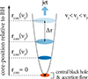 |
Fig. 1. Geometry of the core position of Sagittarius A* as a function of observing frequency. The central SMBH (black dot) launches a jet that is perpendicular to the accretion flow (orange ellipse). The surfaces with optical depth τ = 1 at a given frequency are represented by the blue ellipses. The core-shift between two frequencies is indicated by Δr. Adapted from Figure 4.5 in Lobanov (1996). |
All emission processes have absorption counterparts. In the case of synchrotron emission, the counterpart is synchrotron self-absorption (SSA), in which a photon is absorbed due to its interaction with a charged particle in a magnetic field (B). SSA is the mechanism responsible for the changes in τν along the jet, and is the reason why not all of the synchrotron photons propagating through the jet can escape the source (Ginzburg & Syrovatskii 1969). Low-frequency synchrotron photons (i.e., 22 GHz) suffer stronger absorption by the relativistic electrons in the plasma than high-frequency photons (i.e., 86 GHz). For nonthermal electrons that follow a power-law distribution of particles, the absorption coefficient (αν) has a strong dependence upon frequency (ν; for full details see Eq. (6.53) of Rybicki & Lightman 1979). The absorption coefficient, αν, is expressed as
 (1)
(1)
where C is a constant, B is the magnetic field, and P is the index of the of the particle distribution law of relativistic electrons. At high observing frequencies, the absorption is small, and therefore the plasma is optically thin and we can see “deeper” into the source than at low frequencies. A description for nonthermal electrons is used in this paragraph to illustrate the concept of core-shift. We note that for our work we assume a thermal, relativistic distribution of radiating electrons (as is described in Sect. 2).
Because the displacement of the absolute position of the core with observing frequency is a strong indicator of the presence of a conical or parabolic jet, studying core-shifts is an powerful tool to probe the emission mechanisms around a SMBH. The distance from the central engine to the observed core can be written as
 (2)
(2)
where rcore is the core position relative to the BH as a function of the observing frequency, ν. The index kr depends on jet properties such as the particle density distribution, electron energy spectrum, jet opening angle, and magnetic field. The factor kr = 1 is predicted for SSA with equipartition between the magnetic field energy and the energy density of the relativistic particles (Blandford & Königl 1979). The core-shift, Δr (see Fig. 1), between two observing frequencies, ν1 and ν2, can be expressed as
 (3)
(3)
In previous work using high-precision astrometry, core-shifts have been measured along the jets of many AGNs (e.g., Lara et al. 1994; Lobanov 1998a; Kadler et al. 2004; Hada et al. 2011; Haga et al. 2015; Kovalev et al. 2008; Voitsik et al. 2018). In the case of M81, whose nuclear radio source M81* shares similarities with Sgr A*, core-shift studies have placed constraints on the size of the emission region around M81*, with the central BH located within a region of ±0.2 mas, and confirmed that M81* is a compact core-jet source (Bietenholz et al. 2004). Modeling of the nuclear jet of M81 has also shown nonlinearity in its size-frequency relation and a non-conical shape for the jet (Falcke 1996).
For Sgr A* the presence of a core-shift has been investigated using the Galactic center pulsar (Bower et al. 2015a). The pulsed radio emission of the magnetar was phase-referenced to the core position of Sgr A* using two band-pairs (15–8 GHz and 43–22 GHz). This work places a 3σ upper limit on the core-shift of 0.3 mas cm−1 in right ascension and 0.2 mas cm−1 in declination. Observations of Sgr A* at 43 GHz and 86 GHz with the Korean VLBI Network (KVN) report a core-shift of 0.3 mas cm−1 (Zhao et al. 2017). However, the direction of the core-shift is inconsistent with that measured by Bower et al. (2015a). The authors consider the contribution of the calibrators own core-shift plus blending effects due to the large KVN beamsize (Rioja et al. 2014) to be the reason for the discrepancy.
The goal of this work is to predict the frequency-dependent position of Sgr A*’s radio core and to estimate the core-shift for different jet-plus-disk models. Our predictions are made using three-dimensional general relativistic magnetohydrodynamical (3D GRMHD) simulations, ray-tracing, and scattering screen models. We have chosen to investigate combined emission models of jets plus accretion inflows (Mościbrodzka et al. 2014; Shiokawa 2013) because they reproduce well the observed spectrum and intrinsic size of Sgr A*. We also investigate the evolution of the core-shift as a function of the viewing angle and orientation on the sky, and study the core-shift behavior in the presence of interstellar scattering. First we assume the ideal case in which our models are seen with infinite resolution, then we simulate the effects of observing our models with the Very Long Baseline Array (VLBA).
This paper is organized as follows. Sect. 2 describes the emission models that can explain the observed radiation. Sect. 3 provides context on the effects that interstellar scattering has on Sgr A* observations. Sect. 4 presents our results, discusses the modeling of core-shifts, investigates the effects of an interstellar scattering screen, studies the behavior of cores-shift as a function of the orientation of Sgr A*, and includes the effects of carrying out VLBA observations. Sect. 5 discusses constraints from observations, and future prospects, and Sect. 6 summarizes our conclusions. Lastly, additional material containing a library of model images created for this work, as well as tables with model parameters, is stored in the link provided in Data availability.
2. Disk and jet emission models for Sagittarius A*
Our underlying, dynamical model of plasma flow onto Sgr A* is produced in 3D GRMHD simulations. We assumed that the observed Sgr A* emission is produced by a two component (disk-plus-jet) model. The model consists of a radiatively inefficient accretion flow (RIAF) onto a spinning BH, i.e., a turbulent disk, plus a strongly magnetized, low-density, relativistic outflow, i.e., a jet (Blandford & Znajek 1977; Blandford & Payne 1982). Because the spin of Sgr A* is unconstrained, we used a fiducial spin value of a* = 0.94. Particle heating determines which part of the jet-disk system dominates the appearance. The turbulent plasma inflows and outflows have different amounts of magnetization. Plasma is weakly magnetized in the accretion disk, whereas it is strongly magnetized in the jet outflows. These simulations are described in detail in Shiokawa (2013) and Mościbrodzka et al. (2014).
Next, we used the general relativistic radiative transfer scheme IPOLE (Mościbrodzka & Gammie 2018) to generate synthetic radio maps of the model. The radiative transfer simulations were carried out assuming the following fixed parameters for the Sgr A* system: a BH mass of MBH = 4.5 × 10⁶ M⊙ and a distance, D = 8.6 × 10³ pc, from the observer as was used in Mościbrodzka et al. (2014). These values are slightly different than the results from Abuter (2019). The distance, D, is necessary for the conversion from absolute luminosity to observed flux density. All models were normalized to produce a total flux of 2 Jansky at a frequency of 86 GHz to be consistent with observed fluxes of Sgr A* (Issaoun et al. 2019). The normalization was done by changing the value of the mass unit, ℳ, which translates the mass accretion rate, Ṁ, into physical units of M⊙/year. In practice this means that the matter densities in an entire model are multiplied by a constant scaling density factor. ℳ also changes the magnetic field strength.
We ran IPOLE to integrate the radiative transfer equation including synchrotron emission and SSA. We assumed a thermal, relativistic Maxwell-Jüttner electron distribution function (eDF) for the radiating electrons in both the disk and jet regions. The ratio of the proton-to-electron temperature (Tp/Te) is not followed in the considered GRMHD simulation. Hence, in what follows we parameterize in terms of the plasma parameter β (i.e., the ratio of the gas pressure to magnetic pressure β = Pgas/Pmag), and in terms of some coupling constants, Rhigh and Rlow, so that
 (4)
(4)
The coupling constants, Rhigh and Rlow, describe the proton-to-electron coupling in weakly and strongly magnetized plasma, respectively. For weakly magnetized plasma β ≫ 1 (e.g., inside a turbulent accretion disk), Tp/Te → Rhigh. For strongly magnetized plasma β ≪ 1 (e.g., along a jet), Tp/Te → Rlow. This approach was adopted from Mościbrodzka et al. (2016b) and motivated by studies of electron-proton couplings in collisionless plasma (Howes 2010; Ressler et al. 2015; Chael et al. 2018; Kawazura & Barnes 2018). By increasing the value of Rhigh we can move smoothly from models where the source appearance is dominated by disk emission to models where the source appearance is dominated by jet emission. In this work we do not scan the whole parameter space of Rhigh and Rlow. We chose to investigate two models: a bright disk and a bright jet. Emission models with (Rhigh, Rlow) = (3, 3) result in bright disks. For these disk models, we assume that electrons are strongly coupled to protons both in the disk and in the jet, and that the temperature ratio is Tp/Te = 3 everywhere (Mościbrodzka et al. 2009). In the equatorial plane of the accretion disk the plasma density is highest, and therefore emission from the disk dominates. In contrast, models with (Rhigh, Rlow) = (20, 1) result in bright jets. For these jet models, electrons are weakly coupled to protons in the accretion disk (Tp/Te = 20), but they remain strongly coupled to protons in the jet (Tp/Te = 1); hence, synchrotron emission from the jets overpowers the disk emission.
Another parameter that we changed to generate different models is the inclination (i.e., viewing) angle, i. This is the angle between the observer’s line-of-sight and the BH spin axis as illustrated in Fig. 2. The morphology of the emission models is strongly dependent on i. Findings have shown that i can be partially constrained for the jet models presented here using observations at 86 GHz (Issaoun et al. 2019). Furthermore, we also changed the position angle (PA), which is the orientation of the BH spin axis on the plane of the sky.
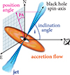 |
Fig. 2. Geometry of the emission models. The angle between the observer’s line-of-sight and the BH spin axis is defined as the inclination angle (i). The orientation of the spin axis on the plane of the sky is the position angle (PA). A completely face-on accretion disk occurs at i = 0°, an edge-on disk is seen at i = 90°. The spin axis points due north when PA = 0°, and due east when PA = 90°, orientation changes east of north (i.e., counterclockwise). |
3. Interstellar scattering model for Sagittarius A*
Studies of Sgr A* at 43 GHz and 86 GHz (e.g., Krichbaum et al. 1993; Lu et al. 2011) have shown that its intrinsic structure starts to be unveiled as the effects of the scatter broadening become less dominant at frequencies ≳43 GHz (Doeleman et al. 2001; Bower et al. 2004; Shen et al. 2005; Bower et al. 2006; Krichbaum et al. 2006). Studies report substructure at micro-arcsecond scales in the emission from Sgr A* at 86 GHz (Brinkerink et al. 2019). Additionally, Issaoun et al. (2019) have obtained the first image of Sgr A* at 86 GHz where the intrinsic source structure has been deconvolved from the effects the interstellar scattering. Using observation of very scattered pulsars within the Galactic center suggest that at least two scattering screens are required to explain the pulsar observations, with one component being within ≤700 pc of the GC and another faraway at ∼2 kpc from Earth (Bower et al. 2014a; Dexter et al. 2017).
When investigating the effects of scattering, there are two important spatial scales to consider: the diffractive scale (rdif) and the refractive scale (rref). Fig. 3 illustrates the scattering screen geometry. The smallest scale on which flux variations due to turbulence happen is rdif. Diffractive scattering leads to scatter-broadening of the source. The image size projected onto the scattering screen is defined as rref (Narayan & Goodman 1989a; Psaltis et al. 2015). Refractive scattering causes substructure in the image and it has already been observed in Sgr A* at 13 mm (Gwinn et al. 2014).
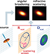 |
Fig. 3. Geometry of the scattering screen. This diagram shows the diffractive (rdif) and refractive (rref) scales, screen-Earth distance (Dscat), screen-Sgr A* distance (Rscat). Modified from Fig. 1 in Psaltis et al. (2018). |
These scales can be written in terms of the observing wavelength, λ, as follows (Psaltis et al. 2018):
 (5)
(5)
 (6)
(6)
where θscat ∼ λ2 gives the angular size of the scattered image of Sgr A* assuming a Gaussian scattering kernel. In the regime where rref > rdif strong scattering occurs. When rdif and rref become comparable, refractive noise (which introduces stochastic changes) needs to be considered when imaging Sgr A* (Johnson et al. 2018).
In this work we used the Python library eht-imaging (Chael et al. 2016) and its module stochastic-optics (Johnson 2016) to simulate the effects of the scattering screen using a scattering model that is physically motivated by observations of Sgr A* (Johnson et al. 2018; Psaltis et al. 2018; Issaoun et al. 2019).
4. Results
Here we present flux density maps of Sgr A* for our disk and jet emission models (Sect. 4.1), we make core-shift predictions for different models without scattering (Sect. 4.2) and then include the effects of interstellar scattering on core-shift modeling (Sect. 4.3). In addition, we investigate the effects of changing the inclination angle and the position angle of Sgr A* (Sect. 4.4), and simulate observations with the VLBA (Sect. 4.5).
4.1. Model radio maps of Sagittarius A*
We studied 14 radiative transfer models with various combinations of parameters as summarized in Table 1. We changed the inclination angle (i) with respect to the observer’s line-of-sight and the proton-to-electron coupling constants (Rhigh and Rlow). We generated maps of the flux density (Sν) for each model at three observing frequencies (ν = 22 GHz, 43 GHz, and 86 GHz) and at seven inclination angles (i = 1°, 15°, 30°, 45°, 60°, 75°, and 90°). We kept the position angle on the sky of the BH spin axis at PA = 0°. Later in this paper, we create maps where the orientation angle is rotated to PA = 45° and to PA = 90° east of north (see Section 4.4).
Model parameters.
The resulting flux density maps are presented in Fig. 4 for disk models, and in Fig. 5 for jet models. The inclinations shown are in steps of Δi = 30°. Nevertheless, for the sake of completeness, additional figures for intermediate inclinations (i = 15°, 45°, and 75°) are included in Sect. B of the support material. The radio maps in Figs. 4 and 5 show the intrinsic image of Sgr A*, angular broadening due to interstellar scattering is thus far not included. We choose to show the square-root of the flux density rather than the flux density in a linear scale so that faint, low-flux regions can be clearly discerned.
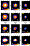 |
Fig. 4. Flux density (Sν) maps of disk models. Rows of panels show disk models with different inclinations (i = 1°, 30°, 60°, and 90°, top to bottom). The position angle on the sky of the BH spin axis is PA = 0° for all models. Columns show the maps at different frequencies (22 GHz, 43 GHz, and 86 GHz, left to right). The FOV for each panel is 120 × 120 GM/c2 (645 × 645 μas). The bottom color bar indicates the flux density in square-root scale, the y axis shows the distance from the BH (located at 0,0) in units of GM/c2, and the top x axis shows that same distance in μas. The green dot represents the position of the intensity weighted centroid. |
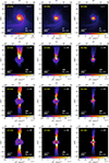 |
Fig. 5. Flux density (Sν) maps of jet models. Rows show jet models with different inclinations with respect to the observer’s line of sight (i = 1°, 30°, 60°, and 90°, top to bottom). The position angle on the sky of the BH spin axis is PA = 0° for all models. Columns show the maps at different frequencies (22 GHz, 43 GHz, and 86 GHz, left to right). The FOV for each panel is 300 × 300 GM/c2 (1600 × 1600 μas). The bottom color bar indicates the flux density in square-root scale, the y axis shows the distance from the BH (located at 0,0) in units of GM/c2, and the top x axis that same distance in μas. The green dot represents the position of the intensity weighted centroid. |
For each emission model at 43 GHz and 86 GHz, we created a snapshot of an area in the Galactic center with dimensions 300 × 300 Rg, where the gravitational radius corresponds to a size of Rg = 6.6 × 1011 cm for Sgr A*. The field of view (FOV) is doubled to 600 × 600 Rg for models at 22 GHz so extended emission at large scales in the jet models can be captured in the maps. In addition, to study the effects of scattering at 22 GHz large FOVs are required due to the large angular broadening produced by the scattering kernel at this frequency. The FOV size and resolution are summarized in Table 2.
Fields of view.
As expected, the appearance of the emission models depends strongly on the assumed electron temperature. In Fig. 4 the emission from Sgr A* is dominated by the disk due to the strong electron-proton coupling in all regions, while in Fig. 5 emission is dominated by the jets due to strong electron-proton coupling occurring in the jet regions.
As we move from the top row to the bottom row in Figs. 4 and 5, the inclination angle, i, changes from almost completely face-on (i = 1°) to completely edge-on (i = 90°). An interesting feature starts to emerge for disk models with high inclination when observed at 86 GHz (Fig. 4, bottom right). Although the disk is viewed edge-on, its appearance reveals a distinct ring-like structure. The extreme gravitational field generated by the BH bends the path followed by the photons radiated by the disk, so light coming from the back side of the accretion disk can be seen by the observer. Sgr A* acts as a gravitational lens that disturbs the geometry of the emission. The noticeable ring is the photon orbit and the central darker area is the shadow of the BH. The left side of the disk is brighter, as indicated by the intensity centroid (green dot) being displaced from the geometrical center of the map. See Sect. 4.2 for a full description of centroid calculations. As matter swirls around the SMBH at relativistic speeds, the plasma on that side of the disk moves toward the observer and the radio emission is Doppler-boosted, and thus appears brighter.
Jet models (Fig. 5) show a different morphology. The accretion disk appears faint compared to emission coming from the polar jets. At intermediate inclinations, emission from the jet pointing toward the observer (which is Doppler-boosted) dominates over the emission coming from the counter-jet (pointing away) and emission originating from the disk. At i = 90°, the emission is bright for both jets above and below the dim disk. In these jet models we cannot discern the boundary of the event horizon even at the highest observing frequency we calculate here because they have a higher optical depth.
4.2. Core-shift modeling without scattering
We obtained the radio core positions at each frequency using the following method. First, we calculated the intensity-weighted centroid of each map (i.e., the image “first moment”) as indicated by the green dots in Figs. 4 and 5. The centroid coordinates (xc, yc) are given by
 (7)
(7)
where (xi, yj) is the location of a given pixel, Si, j is the value of the flux density in that pixel, and the dimensions of the map in pixels are (imax × jmax). The errors in the intensity-weighted centroid position (xc, yc) can be expressed as
 (8)
(8)
 (9)
(9)
where Stot is the total flux density of the map.
Next, we calculated the core position relative to the BH (rcore), illustrated in Fig. 1. This is the offset between the centroid (xc, yc) and the geometrical center of the image (x0, y0) where the BH is located:
 (10)
(10)
The error in the core position rcore is
 (11)
(11)
Starting with Equation (2), we can write the frequency-dependent core position relation to be a power-law function in terms of the wavelength, λ, as is commonly used:
 (12)
(12)
where the power-law index is p = 1/kr, and the coefficient A indicates the amplitude (i.e., amount) of core-shift. For each emission model, we fit a power law to rcore at the three observing wavelengths, 13.6 mm, 7 mm, and 3.5 mm (22 GHz, 43 GHz, and 86 GHz), and calculate p, A, and their errors using the nonlinear least squares fitting method optimize.curvefit from Python. These models do not include scattering. Table 3 summarizes these results. Figure 6 shows the best power-law fits for the intrinsic disk and jet models presented in Figs. 4 and 5.
Power-law parameters for jet and disk models.
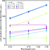 |
Fig. 6. Core position as a function of wavelength for intrinsic jet and disk models. Squares indicate the core position relative to the central BH at 13.6 mm, 7 mm, and 3.5 mm (22/43/86 GHz) for jet models. Colors represent different inclination angles. Circles indicate the core positions for disk models. All models have an orientation of PA = 0°. Solid lines (jets) and dashed lines (disks) show the best-fit power law using a least-squares fitting method. Error bars represent 1σ errors in the core position data. Parameters, fitting errors, and χ2 are summarized in Table 3. The legend indicates the inclination (i) and power-law index (p) for a given model. |
We can see in Fig. 6 that the intrinsic core-shifts of Sgr A* for models with intermediate inclinations (i = 30° ,60°) are larger than core-shifts for i = 1° models or for completely edge-on models (i = 90°). Jet models show a larger amount of core-shift (A) and steeper slope (p) in the power-law relation than disk models. The former follow a power-law function quite well, as is seen from the values in Table 3. This result agrees with predictions of a displacement in the observed cores of AGNs with conical jets (Königl 1981). Falcke & Biermann (1999) predict values of p = 0.9 − 1.1 increasing with inclination. Our results are within the same p range but the slight trend with inclination occurs in the opposite direction, as our p decreases with inclination. This could be due to the jet collimation shape in their analytical work being slightly different from the collimation shape in our 3D GRMHD models. A purely conical jet would yield p = 1.
For jet models, we obtain core positions relative to the BH ranging from rcore ∼ 30 − 400 μas. In contrast, disk models show smaller values ranging from rcore ∼ 9 − 25 μas and have much flatter slopes. If we compare the core-shift of jet models versus disk models, as indicated by the ratio Ajet/Adisk (see Table 4), we can see that it is ∼2–16 times larger. The core-shift is a clear discriminant between jet-dominated and disk-dominated emission models for Sgr A*. Therefore, it can be used as a tool to constrain the values of Rhigh and Rlow, which describe the proton-to-electron coupling on the plasma surrounding Sgr A*.
Ratio of core-shifts.
We should note that even at an inclination of i = 1° the core-shift is detectable in disk models. At i = 0° (completely face-on disk) the core-shift should be 0 due to symmetry in the flux density maps. The bright face-on disk would have similar flux densities to the right and left of the disk. This also explains why the value in jet models at i = 90° (solid magenta line) is so much lower than at intermediate inclinations. At this edge-on inclination, the polar jets have similar (albeit not equal) flux densities above and below the faint accretion disk, which results in the intensity-weighted centroids at all wavelengths being quite close to the geometrical center of the map. Hence, this results in a much flatter power-law slope and smaller value of A.
In particular, we should note that the core position at 13.6 mm and i = 90° (Fig. 6, rightmost magenta square) has a very low value compared to the other inclinations. When examining the flux density maps for this model, although the polar jets exhibit similar flux densities, the northern jet remains brighter at larger scales (Fig. 5, bottom row). However, for the map at 13.6 mm (22 GHz) this feature becomes less noticeable (Fig. 5, bottom left) than at 3.5 mm (86 GHz, bottom right). Hence the centroid location ends up being closer to the geometrical center at 22 GHz. One explanation can be that the full extent of the jets is not being captured at this ν, even though the FOV at 22 GHz was doubled compared to the lower ν (see Table 2). Therefore, we consider the low value of the core position at 22 GHz and the shallowness of the slope p = 0 at i = 90° to be effects of the mapping process rather than having some different underlying physics. This effect “trickles down” to other i = 90° models presented in subsequent sections.
In addition, in the jet model at i = 1° there is a bright arm appearing in the southwest region (see Fig. 5, top row). We consider this feature to be a temporal enhancement of emission in the snapshot image used. This leads to the centroid position being “pulled” slightly southward, and it explains why at this inclination the power-law fit is worse than at intermediate inclinations (see Table 3). The implications of variability in Sgr A* are discussed in Sect. 5.2.
Scattering kernel parameters.
4.3. Core-shift modeling including scattering
The scattering model produces an anisotropic Gaussian that scales as λ2. This Gaussian can be parameterized in terms of the full width at half-maximum (FWHM) sizes along the major and minor axes (θmaj, 0 and θmin, 0), and the position angle on the sky of the Gaussian (PAG). They are given at a reference wavelength λ0 of 1 cm. The parameter values of our scattering screen model are summarized in Table 5. The distances from the scattering screen to Sgr A* (Rscat) and from the scattering screen to the observer (Dscat), as illustrated in Fig. 3 are taken from observations of the Galactic center. We use the inner scale (rin) for the power spectrum of the energy-density fluctuations in the scattering screen, and a power-law index (α) for that power-spectrum generated by turbulence in the screen. All values are adopted from Johnson et al. (2018).
Using the Python library eht-imaging (Chael et al. 2016) and stochastic-optics (Johnson 2016), we convolved our intrinsic model images of Sgr A* (presented in Figs. 4 and 5) with the scattering kernel to produce angular broadening. Then, we generated a refractive phase screen that introduces stochastic variations in the flux density (i.e., “speckles”) using random numbers as Fourier components. The final scattered maps of Sgr A* include refractive scattering and diffractive scattering. An example for a jet model, J30, is shown in Figure 7. The panels on the first row show the intrinsic Sgr A* model maps, the second row shows the scatter-broadened image due to the anisotropic kernel with parameters defined in Table 5, and the last row displays the final scattered image of Sgr A* incorporating stochastic effects due to refractive noise. A library of maps showing the effects of scattering for jet models and disk models is included in the support material.
As is seen in Fig. 7, at long wavelengths (13.6 mm/22 GHz) Sgr A* is heavily broadened (almost engulfing the whole FOV) due to the high level of diffractive scattering (Fig. 7, first column). Even with an orientation of PA = 0° (i.e., the polar jet runs in the north-south (N-S) direction and is nearly perpendicular to the scattering Gaussian with PAG ∼ 82°), most of the angular broadening occurs along the east-west (E-W) direction and the jet features get completely blurred out. Interstellar scattering is very dominant at this observing wavelength. At the shortest wavelength (3.5 mm/86 GHz, Fig. 7 last column), the plasma starts becoming optically thin so the jet begins to be revealed as a faint feature in the north direction, the counter-jet remains unseen.
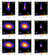 |
Fig. 7. Jet model (J30) including scattering. Each column shows a jet model with inclination i = 30° at 22 GHz, 43 GHz, and 86 GHz (left to right). The position angle on the sky is PA = 0°. Rows from top to bottom show the intrinsic 3D-GRMHD jet model, the scatter-broadened image, and the average image including refractive scattering. Note that the FOV for images at 22 GHz including scattering (left column) is doubled compared to the FOV at 43 GHz and 86 GHz. The color stretch is also different. The intrinsic model panels display the square-root of the flux density (top row). The scattered maps show a linear scale (second and third rows). The green dot indicates the centroid of each image. Black cross-hairs (second and third rows) indicate the location of the centroid of the model before scattering. |
By inspecting the locations of the centroids for each map (green dots) and comparing them to the centroids prior to scattering (black cross-hairs), we can see that scattering appears to have no effect on the centroid position. This is due to the effect being very small so that it would require zooming in to the central area of the map extremely closely. There are minor changes in the centroid location that become more evident when plotting the core position as a function of λ before and after scattering, as is shown in Fig. 8.
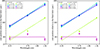 |
Fig. 8. Core position as a function of wavelength for scattered jet models. Left panel: Squares indicate the core position relative to the central BH at 13.6 mm, 7 mm, and 3.5 mm (22/43/86 GHz) for unscattered jet models. Triangles indicate the core position for jet models that have been scattered with the kernel. Colors represent different inclination angles (i) with respect to the observer’s line of sight. For all models, the orientation on the sky of the spin axis is PA = 0°. Solid lines (jet models) and dashed lines (jets scattered with the kernel) show the best-fit power law using a least-squares fitting method. Error bars indicate 1σ uncertainty in the core position data points. Errors in the fit parameters and χ2 are summarized in Table C.1 of the support material. The values for the inclination (i) and the power-law index (p) are given in the legend. Right panel: Same as the left but showing jet models (squares) scattered with the kernel and also including refractive scattering (diamonds). |
In Fig. 8 the left panel shows the intrinsic jet models (squares, solid lines) and the jet models after simulating the effects of the scattering kernel (triangles, dashed lines). The right panel shows the same intrinsic jet models compared to scattered models that include scatter broadening plus refractive scattering (diamonds, dashed lines). After accounting for scattering these jet models still fit very well a power-law relation. Adding refractive scattering at these wavelengths (Fig. 8, right panel) has a negligible effect in the core-shift when comparing it to the effect of purely angular broadening due to the kernel (Fig. 8, left panel). For our study of core-shift as a function of inclination angle and position angle, we present the effects of scatter broadening plus refractive scattering at these λ. This decision is also motivated by results of Johnson et al. (2018) suggesting that refractive noise becomes dominant over the intrinsic structure of Sgr A* for λ > 13 mm and that it is less dominant than previously thought at 1.3 mm, so we want to explore the effects of refractive noise within that range of λ. We find that even when jet features are completely “blurred out” by the scattering screen (Fig. 7), a core-shift measurement is still retrievable. Thus, the presence of a scattering screen has negligible effects on core-shift estimates.
4.4. Effects of changing the position angle
In Sections 4.1–4.3 we modeled core-shifts assuming a position angle of PA = 0°. In this section we investigate how changing the orientation of Sgr A* to other PAs affects the core-shift. We change the position angle of the BH spin axis in the direction east of north (i.e., rotate counterclockwise) to PA = 0°, 45°, 90° while keeping the inclination angle, i, constant and the orientation of the scattering kernel unchanged (PAG = 81.9°). We repeat the process for all inclinations and emission models.
We present model J75 as an example. Figure 9 shows jet model with PA = 0°, 45°, 90°. Figure 10 shows the scattered images with corresponding PA orientations. The appearance of Sgr A* becomes more elongated as the PA increases. In the extreme case where the spin axis has PA = 90° (Fig. 10, bottom row), the jets almost line-up completely with the major axis of the scattering Gaussian (ΔPA ∼ 8°), as a consequence Sgr A* is highly broadened in the E-W direction.
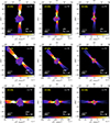 |
Fig. 9. Unscattered jet model (J75) with different position angle orientations. Each column shows a jet model with inclination i = 75° at frequencies of 22 GHz, 43 GHz, and 86 GHz (left to right). Rows from top to bottom show the unscattered jet model with position angles of the BH spin axis of PA = 0° ,45° ,90° (rotated east of north counterclockwise). Their identifications are J75, J75#, J75*, respectively. The FOV of the 22 GHz images (left column) is doubled compared to the FOV at 43 GHz and 86 GHz. The green dot indicates the intensity-weighted centroid of each image. |
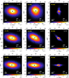 |
Fig. 10. Scattered jet model (J75) with different position angle orientations. Each column shows a scattered jet model with inclination i = 75° at frequencies of 22 GHz, 43 GHz, and 86 GHz (left to right). Rows from top to bottom show the scattered jet model including refractive noise with position angles of the BH spin axis of PA = 0° ,45° ,90° (rotated east of north counterclockwise). Their identifications are J75, J75#, and J75*, respectively. The scattering screen remains fixed at PAG = 81.9°. The FOV of the 22 GHz images(left column) is doubled compared to the FOV at 43 GHz and 86 GHz. The green dot indicates the intensity-weighted centroid of each image. Black cross-hairs indicate the location of the intensity-weighted centroid of the unscattered jet model. |
Using centroid calculations, we can investigate the evolution of the core-shift parameters, A and p, as a function of inclination angle for the three orientations (PA = 0° ,45° ,90°) of the jets as presented in Figure 11. Comparing intrinsic jet models with jet models including angular broadening plus refractive noise for PA = 0° shows that differences in the core-shift are negligible (blue squares vs. green triangles in Fig. 11, bottom left). However, changing the jet orientation with respect to the scattering screen affects core-shift values, with increasing PA the core-shift of scattered jet models starts to deviate from the intrinsic model values (see Fig. 11, top left). This suggests that scattering effects become negligible when the source intrinsic PA is close to perpendicular to the PA of the scattering kernel. As Sgr A*’s jet orientation gets aligned with the scattering kernel, the effect gets larger. However, the overall core-shift amplitude A decreases with increasing PA. In addition, larger core-shift amplitudes occur at intermediate inclinations (i = 30° ,45°) for all jet model orientations.
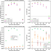 |
Fig. 11. Core-shift parameters of all models as a function of inclination angle for different spin axis orientations. Top left: Core-shift amplitude (A) versus inclination angle (i) for different position angle (PA) orientations of the BH spin axis. Diamonds represent A values for jet models with PA= 0°, 45°, 90° (shown in different colors) which have been scattered by the broadening kernel including refractive noise. Top right: Same as the left, but displaying the core-shift slope (p), which is the index of the power-law relation rcore = Aλp (inverted triangles, scattered). Bottom left: Core-shift amplitude (A) versus inclination angle (i) for disk models (orange circles), scattered disk models ( brown diamonds), jet models (blue squares) and scattered jet models (green inverted triangles) all at a single position angle of PA = 0°. Bottom right: Same as the left plot, but displaying the core-shift slope (p) for the same models. All plots include 1σ error bars obtained from the power-law fits. |
The core-shift slope, p, has a value slightly larger than 1 (green triangles) for PA = 0°, about 1 for PA = 45° (magenta triangles) and lower than 1 for PA = 90° (purple triangles), so the slope of the power law (Equation (12)) becomes less steep as the position angle increases (see Fig. 11, top right). In addition, p starts decreasing at inclinations i ≥ 45°. Although there is a downward trend, it is important to note that the fits for models with i = 90° have much larger error bars (see Fig. 11, top right). At i = 90° we get two negative p values which are caused by two effects in our calculations. First, at this edge-on inclination the polar jets with similar flux densities above and below the faint accretion disk artificially generate centroids very close to the geometrical center of the map, thus p ∼ 0 (as discussed in Sect. 4.2). Secondly, as the PA increases the value of p is further brought down, due to the effect of changing the orientation of the jets with respect to the scattering screen PA, resulting in negative values (rightmost magenta/purple triangles). Negative p values for the power-law index contradict the physics expected from jet models and observations of AGNs. SSA changes the τν along the jet, at short λ the plasma becomes optically thin, so we can see deeper into the core than at longer λ. Therefore, we consider these outlier points (with i = 90°) not physically meaningful as discussed in Sect. 4.2.
If we compare jet and disk models it is clear that the former have much larger core-shifts (Fig. 11, bottom left), with jet models reaching a peak value of A ∼ 241 μas cm−1 while for disk models A ∼ 25 μas cm−1. The relation of core position as a function of wavelength does not fit a power law well for disk models (Fig. 11, bottom right). This means that observations of core-shift at millimeter wavelengths are a powerful tool to discriminate between jet and disk models for Sgr A*.
4.5. Simulating VLBI observations
In Sections 4.2–4.4 we have shown the core-shift behavior in an ideal case where our models are seen with infinite resolution. Here we investigate the effects of observing our models with the VLBA. This array has the capability to perform fast-frequency switching observations with high resolution (i.e., quickly cycling between different ν while observing a source) and can observe at the ν of our study. A follow-up paper investigates core-shift constraints obtained from archival VLBA observations at such ν (Fraga-Encinas et al., in prep.)
For this purpose we took the models including scatter broadening and refractive scattering (as are presented in Section 4.3) and convolved them with an idealized VLBA beam for Sgr A* at our ν of interest (see Table 6). The point-spread-function or “dirty beam” of the VLBA is the response of this array to an observation. For our simulations we took as our beam an idealized CLEAN beam, which is the elliptical Gaussian fitted to the primary lobe of the dirty beam, with values adopted from Lu et al. (2011). As an example we took the J30 model (shown in Fig. 7) and convolved it with our VLBA beam. Figure 12 illustrates the effects of observing Sgr A* with this array. The panels on the first row show the intrinsic emission of Sgr A*, the second row shows the scatter-broadened image incorporating refractive noise, and the last row shows the convolution of the scattered image with the idealized VLBA beam.
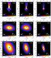 |
Fig. 12. Jet model (J30) including scattering as observed by the VLBA. Each column shows a jet model with inclination i = 30° at 22 GHz, 43 GHz, and 86 GHz (left to right). The position angle on the sky is PA = 0°. Rows from top to bottom show the intrinsic 3D-GRMHD jet model, the jet model with scatter-broadening plus refractive scattering, and at the bottom the observed jet. Note that for images at 22 GHz (left column), and the observed jets at all frequencies have a larger FOV. The color stretch is also different. The intrinsic model panels display the square-root of the flux density (top row). The scattered and observed maps show a linear scale (second and third rows). The green dot indicates the centroid of the unobserved models (first and second rows). The purple diamond indicates the centroid of the observed models (third row). Black cross-hairs indicate the location of the centroid of all models before scattering. |
As is seen in Fig. 12, the morphology of Sgr A*’s emission changes when observed by the VLBA. At all ν its appearance is broadened and the PA of the image varies as a result of the observing beam shape and orientation. Looking at the rightmost column (maps at 3.5 mm/86 GHz), the jet is still discernible in the unobserved scattered image (middle panel). However, when this model is observed the jet-feature gets washed out and becomes unresolved (bottom panel). In addition, any anisotropies in the flux due to refractive scattering are smoothed out by the beam.
The VLBA is an array located in the northern hemisphere. Due to the low declination of Sgr A* (i.e., it never rises high on the sky for this array), the u,v-coverage is elliptical and the angular resolution of the observing beam is lower in the north-south direction than in the east-west direction (see Table 6). The longest baseline is in the east-west direction, about 8600 km, between Hawaii and the Virgin Islands. This means that the array cannot resolve well source structure that lines up with the major axis of the beam, as given by PAB.
VLBA beam shape.
We repeated the calculations for the core position as a function of λ that were shown in Fig. 8, but now including the effects of observing our jet models with the VLBA. The results are presented in Fig. 13. Comparing the unobserved versus the observed models (Fig. 13, left panel), we can see that simulating the angular broadening with the VLBA beam causes a decrease in the core-shift magnitude and a decrease in the steepness of the power-law fit, the p index becomes smaller. Comparing observed jet models with and without scattering also shows a small decrease in the steepness of the fit and core-shift magnitude (Fig. 13, right panel). Thus, it is important to include the effects of observing with a VLBI array in our estimations of the core-shift for future comparisons with real-life observations. In addition, we investigated if the trends seen in Fig. 6 for intrinsic jet and disk models follow the same behavior in their counterpart observed models as is illustrated in Fig. 14. In both cases, the intrinsic disk models and the observed disk models show significantly smaller core-shifts than the jet models.
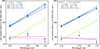 |
Fig. 13. Core position as a function of wavelength for observed jet models. Left panel: Squares indicate the core position relative to the central BH at 13.6 mm, 7 mm, and 3.5 mm (22/43/86 GHz) for unscattered jet models. Crosses indicate the core position for observed and unscattered jet models. Colors represent different inclination angles (i) with respect to the observer’s line of sight. For all models, the orientation on the sky of the spin axis is PA = 0°. Solid lines (jet models) and dashed lines (jets observed with the VLBA) show the best-fit power law using a least-squares fitting method. Error bars indicate 1σ uncertainty in the core position data points. Errors in the fit parameters and χ2 are summarized in Table D.1 in the support material. The values for the inclination (i) and the power-law index (p) are given in the legend. Right panel: Same as the left but showing observed jet models (crosses) and observed jet models scattered with the kernel and including refractive scattering (hexagons). |
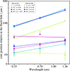 |
Fig. 14. Core position as a function of wavelength for observed jet and observed disk models. Crosses indicate the core position relative to the central BH at 13.6 mm, 7 mm, and 3.5 mm (22/43/86 GHz) for observed jet models. Colors represent different inclination angles. Stars indicate the core positions for observed disk models. All models have an orientation of PA = 0°. Solid lines (jets) and dashed lines (disks) show the best-fit power law using a least-squares fitting method. Error bars represent 1σ errors in the core position data. Parameters, fitting errors and χ2 are summarized in Tables D.1 and D.2 in the support material. The legend indicates the inclination (i) and power-law index (p) for a given model. |
In Fig. 11 we show the core-shift parameters, A and p, as a function of the inclination, i, for different PA orientations of Sgr A*. We now repeat this exercise for observed models and present the results in Fig. 15 for comparison. The core-shift amplitude, A, decreases with increasing PA for both jet models (squares) and observed jet models (crosses) as shown in Fig. 15 (top left). However, and this is a crucial point, this decrease is not homogeneous for the different orientations. Observed jet models with PA = 0° (green crosses) have a much larger decrease in the core-shift magnitude with respect to the unobserved jet models (green squares) than observed models at PA = 90° (blue crosses) with respect to their unobserved counterparts (blue squares). This means that for observed jet models the intensity-weighted centroid of the emission is located more upstream along the jet (i.e., closer to the BH) than for unobserved jet models. The observed core-shift is smaller.
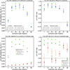 |
Fig. 15. Core-shift parameters of observed models as a function of inclination angle for different spin axis orientations. Similar to Fig. 11 but including models observed by the VLBA. Top left: Core-shift amplitude (A) versus inclination angle (i) for different position angle (PA) orientations of the BH spin axis. Squares represent A values for scattered jet models with PA = 0°, 45°, 90° (shown in different colors) which have been scattered by the broadening kernel including refractive noise, crosses are the same scattered jet models but observed by the VLBA. Top right: Same as the left, but displaying the core-shift slope (p), which is the index of the power-law relation rcore = Aλp. Bottom left: Core-shift amplitude (A) versus inclination angle (i) for scattered disk models (brown diamonds), observed scattered disk models (orange plus markers), scattered jet models (green squares) and observed scattered jet models (dark green crosses) all at a single position angle of PA = 0°. Bottom right: Same as the left plot, but displaying the core-shift slope (p) for the same models. All plots include 1σ error bars obtained from the power-law fits. |
This effect can be explained if we consider the alignment of the VLBA beam and the jets. The beam orientation ranges from PAB = 12.1° −20.1° (see Table 6), which are low values. When the PA of the model is close to lining up with the orientation of the beam PAB the decrease in the observed core-shift is more pronounced than when PA and PAB are near perpendicular to each other. This effect is attributed to having a poorer resolution in the north-south direction than in the east-west direction due to the elliptical nature of the beam. Furthermore, the core-shift of observed jet models has its largest values at intermediate inclinations (i = 30° ,45°) with amplitudes of A ∼ 213 μas cm−1 and A ∼ 216 μas cm−1, respectively.
The same trend is seen in the core-shift slope p (Fig. 15, top right), where the steepness of p is reduced more prominently at orientations of PA = 0° compared to PA = 90°. Omitting the outlier p values at inclination i = 90° (as discussed in Section 4.2), the power-law index ranges from p ∼ 0.8 − 0.9.
Regarding the observed disk models, the bottom left panel of Fig. 15 (orange plus markers), shows that A is very low in comparison with the observed jet models, and it has a peak value of A ∼ 29 μas cm−1. Simulating a VLBA observation of disk models shows no significant changes in the value of A compared to intrinsic disk models. It is also relevant that no kind of disk model fits a power law well for the core-shift as a function of λ (bottom right panel).
5. Discussion
Here we discuss constraints from observations of Sgr A* (Sect. 5.1) and how future studies can extend the results presented in this work (Sect. 5.2).
5.1. Constraints from observations
Using VLBI observations the source orientation and type of emission model can be constrained. Work by Issaoun et al. (2019) presents the first intrinsic image of Sgr A* at 3.5 mm from observations with GMVA plus ALMA. An intrinsic size of 120 ± 34 μas (major axis) and axial ratio of 1.2 is reported. The axial ratio indicates a fairly symmetrical source geometry. The authors compare several emission models to the observational constraints, among their models they consider the disk and jet models presented in this work.
Disk models for which (Rhigh, Rlow) = (3, 3) do not match the size and asymmetry limits from 3.5 mm observations. However, jet-dominated models with (Rhigh, Rlow) = (20, 1) fit the constraints but only at inclinations of i ≲ 20°.
In addition, observations of Sgr A* with the East Asian VLBI Network (EAVN) at 13.6 mm and 7 mm have obtained an intrinsic size of 704 ± 102 μas (major axis) and axial ratio of 1.2 ± 0.2, and 300 ± 25 μas (major axis) and axial ratio of 1.3 ± 0.2, respectively (Cho et al. 2022). They choose to compare the intrinsic structure of Sgr A* to RIAF models with a thermal plus nonthermal electron distribution function. Their motivation for using a nonthermal component of synchrotron emission is due to the observed excess flux in the spectral energy distribution of Sgr A* at 13.6 mm and 7 mm. Emission models with inclination i = 20° and i = 60° are compared to axial ratio measurements. The results indicate that low inclinations are preferred, somewhere in the range of i ∼ 30°–40°. From near infrared observations of flaring events in Sgr A*, orbital parameters of the observed “hot spots” in the innermost accretion region of Sgr A* yield an inclination of i ≲ 25° (Abuter 2018).
From Fig. 11 (left panels) we can estimate a maximum theoretical value for the core-shift of ideal jet models including refractive scattering of A = 241.65 ± 1.93 μas cm−1, corresponding to an inclination of i = 30° (see Table C.1 in the support material). When simulating VLBA observations (Fig. 15) the maximum core-shift is A = 215.57 ± 1.95 μas cm−1 at i = 45° (see Table D.1 in the support material).
5.2. Future prospects
Firstly, the work presented here is not a study on time variability. Our findings on the core-shift are based on snapshots of each model. Previous work has studied the variability of the centroid position due to refractive scattering and estimated the image wander at 1.3 mm to be 0.53 μas using the same scattering model we use, as well as demonstrated that the effects of refractive image wander can be mitigated by averaging images over multiple observations (Zhu et al. 2019). In our work we show that the ability to recover core-shift measurements is not impaired by the presence of a scattering screen or when observing with the VLBA. The largest uncertainties we obtain in core-shift calculations are of the order of ∼5 μas, so we are confident that further studies in which multiple scattered images of Sgr A* are averaged would still yield measurable core-shifts, and improved power-law fits since inhomogeneities in the emission will be mitigated.
On timescales ranging from intra-day to several months, Sgr A* displays variable emission at radio, IR and X-ray wavelengths (Macquart & Bower 2006; Yusef-Zadeh et al. 2009; Akiyama et al. 2013). The effects of intrinsic source variability (e.g., flaring events or hot spots) could likely impact core-shift measurements because time lags between flare peaks have already been observed at cm/mm wavelengths (Yusef-Zadeh et al. 2008; Brinkerink et al. 2015). Multi-epoch studies have established that temporal variability of the core-shift magnitude seems to be a common phenomenon in AGNs, and that there is a strong dependence between the core position and its flux density (Plavin et al. 2019). Monitoring of Sgr A* during its active state in 2019 has shown temporal variability of its flux density and its intrinsic source size (Cheng et al. 2023). Thus, the relation between intrinsic source variability and the core-shift of Sgr A* should be further investigated.
For the scope of this paper, we have presented results for dynamical models that include a combination of an ADAF disk plus a mildly relativistic jet with a thermal electron distribution. These radiatively inefficient accretion flow models are Standard And Normal Evolution models (SANE, Narayan et al. 2012) and have low-power jets. It remains to be studied how our core-shift predictions compare to core-shifts from models with a strong disk, strong jet, models where electrons in the jet follow a combination of thermal plus nonthermal power-law distribution (Davelaar et al. 2018), or Magnetically Arrested Disk models (MAD, Bisnovatyi-Kogan & Ruzmaikin 1976; Igumenshchev et al. 2003; Narayan et al. 2003; McKinney et al. 2012). Jets of MAD models are more powerful than jets of SANE models and have a wider jet-funnel opening. It is reasonable to think that core-shifts of MAD models could yield different results than our SANE models. However, we would not expect the core-shifts of disk-dominated versus jet-dominated MAD models to be fundamentally different from those presented here.
In the future, this work can be extended by using the core-shift to constrain the Rhigh and Rlow values of Sgr A* emission models and get better parameter estimates from BH images (EHTC 2022c) taken by current and planned EHT arrays, or by prospective space VLBI missions like the Event Horizon Imager (Roelofs et al. 2021). Another avenue of exploration can be to compare the core-shift predictions presented on this study with available VLBI observations of Sgr A* that were specifically designed to measure core-shifts using the so-called phase-referencing technique (Middelberg et al. 2005). Such an investigation has been carried out using archival VLBA observations and will be presented in a follow-up paper.
6. Summary
In this work we have made predictions about the frequency-dependent position of Sgr A*’s radio core and estimated the core-shift for different jet-plus-disk models. We have used 3D GRMHD simulations, ray-tracing and a scattering model to generate flux density maps of Sgr A* at three frequencies: 22/43/86 GHz. We have studied the evolution of core-shift as a function of the inclination angle and position angle on the sky, and investigated the effects of interstellar scattering and of simulating observations with the VLBA.
We conclude that the core-shift is a clear discriminant between jet-dominated and disk-dominated emission models. It can also be used to constrain the geometry of Sgr A*, such as its inclination and orientation on the sky. Our jet emission models show significantly larger core-shifts than disk models at all inclination angles, in some cases by a factor of 16.
Jet models produced in GRMHD simulations closely follow a power-law relation for the frequency-dependent position of Sgr A*’s radio core and agree with previous predictions of AGNs with conical and parabolic jets (Blandford & Königl 1979; Falcke 1996; Falcke & Biermann 1999). Our disk models do not fit a power-law relation well and their core-shifts are fairly insensitive to changes in the inclination angle. The core-shift is retrievable even in the presence of an interstellar scattering screen located between Earth and Sgr A*. This scattering kernel is responsible for the angular broadening (blurring) and stochastic changes (refractive noise) observed in Sgr A* images. In jet-dominated emission models, the core-shift amplitude decreases as the orientation of the BH spin axis increases from PA = 0° to 90° (east of north).
Scattering effects become negligible when the intrinsic PA of the Sgr A* jet model is close to perpendicular to the PA of the scattering kernel. As the Sgr A*’s jet orientation gets aligned with the scattering kernel, the effect gets larger. Additionally, the largest core-shift amplitudes occur at intermediate inclinations (i = 30° ,45°) for all jet model orientations.
We also obtain a maximum theoretical estimate for the core-shift of jet models including refractive scattering of A = 241.65 ± 1.93 μas cm−1, with this peak value occurring at an inclination of i = 30° in the ideal case. When simulating observations with the VLBA, the maximum core-shift is A = 215.57 ± 1.95 μas cm−1 at i = 45°. Therefore, obtaining core-shifts from multiwavelength observations gives us the means to further constrain the geometry and emission mechanisms of the plasma surrounding Sgr A*, and it can be viewed as a great tool to shed light on an open-ended debate of disk versus jet models of emission.
Data availability
A library of model images created for this work and tables with model parameters is available at https://zenodo.org/records/15520877.
Acknowledgments
We thank the anonymous referee(s) for providing comments to improve the quality of our study. We are grateful to the Event Horizon Telescope Publication Committee, Tomohisa Kawashima, Ilje Cho and Michael D. Johnson for their useful comments when reviewing this work. This research is partially supported by the NWO Spinoza Prize awarded to H. Falcke and by the ERC Synergy Grant “BlackHoleCam: Imaging the Event Horizon of Black Holes” awarded to H. Falcke, M. Kramer and L. Rezzolla, Grant 610058. Software: eht-imaging python library (Chael et al. 2016), Stochastic Optics (Johnson et al. 2018), IPOLE code (Mościbrodzka & Gammie 2018), Python, NumPy (Harris et al. 2020), SciPy, Matplotlib (Hunter 2007), Astropy, Adobe InDesign.
References
- Akiyama, K., Takahashi, R., Honma, M., Oyama, T., & Kobayashi, H. 2013, PASJ, 65, 91 [NASA ADS] [Google Scholar]
- Balick, B., & Brown, R. L. 1974, ApJ, 194, 265 [NASA ADS] [CrossRef] [Google Scholar]
- Ball, D., Özel, F., Psaltis, D., & Chan, C.-K. 2016, ApJ, 826, 77 [NASA ADS] [CrossRef] [Google Scholar]
- Bardeen, J. M. 1973, in Black Holes (Les Astres Occlus), eds. C. Dewitt, & B. S. Dewitt, 215 [Google Scholar]
- Bietenholz, M. F., Bartel, N., & Rupen, M. P. 2004, ApJ, 615, 173 [NASA ADS] [CrossRef] [Google Scholar]
- Bisnovatyi-Kogan, G. S., & Ruzmaikin, A. A. 1976, Ap&SS, 42, 401 [NASA ADS] [CrossRef] [Google Scholar]
- Blandford, R. D., & Königl, A. 1979, ApJ, 232, 34 [Google Scholar]
- Blandford, R. D., & Payne, D. G. 1982, MNRAS, 199, 883 [CrossRef] [Google Scholar]
- Blandford, R. D., & Znajek, R. L. 1977, MNRAS, 179, 433 [NASA ADS] [CrossRef] [Google Scholar]
- Bower, G. C., Falcke, H., Herrnstein, R. M., et al. 2004, Science, 304, 704 [Google Scholar]
- Bower, G. C., Goss, W. M., Falcke, H., Backer, D. C., & Lithwick, Y. 2006, ApJ, 648, L127 [NASA ADS] [CrossRef] [Google Scholar]
- Bower, G. C., Deller, A., Demorest, P., et al. 2014a, ApJ, 780, L2 [Google Scholar]
- Bower, G. C., Deller, A., Demorest, P., et al. 2015a, ApJ, 798, 120 [CrossRef] [Google Scholar]
- Brinkerink, C. D., Falcke, H., Law, C. J., et al. 2015, A&A, 576, A41 [NASA ADS] [CrossRef] [EDP Sciences] [Google Scholar]
- Brinkerink, C. D., Müller, C., Falcke, H. D., et al. 2019, A&A, 621, A119 [NASA ADS] [CrossRef] [EDP Sciences] [Google Scholar]
- Broderick, A. E., & Loeb, A. 2006, MNRAS, 367, 905 [Google Scholar]
- Broderick, A. E., Loeb, A., & Narayan, R. 2009, ApJ, 701, 1357 [NASA ADS] [CrossRef] [Google Scholar]
- Chael, A. A., Johnson, M. D., Narayan, R., et al. 2016, ApJ, 829, 11 [Google Scholar]
- Chael, A., Rowan, M., Narayan, R., Johnson, M., & Sironi, L. 2018, MNRAS, 478, 5209 [NASA ADS] [CrossRef] [Google Scholar]
- Chael, A., Narayan, R., & Johnson, M. D. 2019, MNRAS, 486, 2873 [NASA ADS] [CrossRef] [Google Scholar]
- Chan, C.-K., Psaltis, D., Özel, F., Narayan, R., & Sadowski, A. 2015, ApJ, 799, 1 [NASA ADS] [CrossRef] [Google Scholar]
- Cheng, X., Cho, I., Kawashima, T., et al. 2023, Galaxies, 11, 46 [Google Scholar]
- Cho, I., Zhao, G.-Y., Kawashima, T., et al. 2022, ApJ, 926, 108 [NASA ADS] [CrossRef] [Google Scholar]
- Davelaar, J., Mościbrodzka, M., Bronzwaer, T., & Falcke, H. 2018, A&A, 612, A34 [NASA ADS] [CrossRef] [EDP Sciences] [Google Scholar]
- Davies, R. D., Walsh, D., & Booth, R. S. 1976, MNRAS, 177, 319 [NASA ADS] [Google Scholar]
- Dexter, J., & Fragile, P. C. 2013, MNRAS, 432, 2252 [NASA ADS] [CrossRef] [Google Scholar]
- Dexter, J., Deller, A., Bower, G. C., et al. 2017, MNRAS, 471, 3563 [Google Scholar]
- Doeleman, S. S., Shen, Z.-Q., Rogers, A. E. E., et al. 2001, AJ, 121, 2610 [Google Scholar]
- Doeleman, S. S., Weintroub, J., Rogers, A. E. E., et al. 2008, Nature, 455, 78 [NASA ADS] [CrossRef] [Google Scholar]
- Doeleman, S. S., Fish, V. L., Broderick, A. E., Loeb, A., & Rogers, A. E. E. 2009, ApJ, 695, 59 [CrossRef] [Google Scholar]
- Doeleman, S. S., Fish, V. L., Schenck, D. E., et al. 2012, Science, 338, 355 [NASA ADS] [CrossRef] [Google Scholar]
- EHTC (Akiyama, K., et al.) 2019, ApJ, 875, L1, Paper I [Google Scholar]
- EHTC (Akiyama, K., et al.) 2022a, ApJ, 930, L12 [NASA ADS] [CrossRef] [Google Scholar]
- EHTC (Akiyama, K., et al.) 2022b, ApJ, 930, L16 [NASA ADS] [CrossRef] [Google Scholar]
- EHTC (Akiyama, K., et al.) 2022c, ApJ, 930, L17 [NASA ADS] [CrossRef] [Google Scholar]
- Falcke, H. 1996, ApJ, 464, L67 [Google Scholar]
- Falcke, H., & Biermann, P. L. 1999, A&A, 342, 49 [NASA ADS] [Google Scholar]
- Falcke, H., & Markoff, S. 2000, A&A, 362, 113 [NASA ADS] [Google Scholar]
- Falcke, H., & Markoff, S. B. 2013, Class. Quant. Grav., 30, 244003 [Google Scholar]
- Falcke, H., Goss, W. M., Matsuo, H., et al. 1998, ApJ, 499, 731 [NASA ADS] [CrossRef] [Google Scholar]
- Falcke, H., Melia, F., & Agol, E. 2000, ApJ, 528, L13 [Google Scholar]
- Fish, V. L., Doeleman, S. S., Beaudoin, C., et al. 2011, ApJ, 727, L36 [Google Scholar]
- Fish, V. L., Johnson, M. D., Doeleman, S. S., et al. 2016, ApJ, 820, 90 [Google Scholar]
- Genzel, R., Eisenhauer, F., & Gillessen, S. 2010, Rev. Mod. Phys., 82, 3121 [Google Scholar]
- Ghez, A. M., Salim, S., Weinberg, N. N., et al. 2008, ApJ, 689, 1044 [Google Scholar]
- Gillessen, S., Eisenhauer, F., Trippe, S., et al. 2009, ApJ, 692, 1075 [NASA ADS] [CrossRef] [Google Scholar]
- Ginzburg, V. L., & Syrovatskii, S. I. 1969, ARA&A, 7, 375 [NASA ADS] [CrossRef] [Google Scholar]
- Goddi, C., Falcke, H., Kramer, M., et al. 2017, Int. J. Mod. Phys. D, 26, 1730001 [Google Scholar]
- Gold, R., McKinney, J. C., Johnson, M. D., & Doeleman, S. S. 2017, ApJ, 837, 180 [Google Scholar]
- GRAVITY Collaboration (Abuter, R., et al.) 2018, A&A, 618, L10 [NASA ADS] [CrossRef] [EDP Sciences] [Google Scholar]
- GRAVITY Collaboration (Abuter, R., et al.) 2019, A&A, 625, L10 [NASA ADS] [CrossRef] [EDP Sciences] [Google Scholar]
- Gwinn, C. R., Kovalev, Y. Y., Johnson, M. D., & Soglasnov, V. A. 2014, ApJ, 794, L14 [Google Scholar]
- Hada, K., Doi, A., Kino, M., et al. 2011, Nature, 477, 185 [NASA ADS] [CrossRef] [Google Scholar]
- Haga, T., Doi, A., Murata, Y., et al. 2015, ApJ, 807, 15 [NASA ADS] [CrossRef] [Google Scholar]
- Harris, C. R., Millman, K. J., van der Walt, S. J., et al. 2020, Nature, 585, 357 [NASA ADS] [CrossRef] [Google Scholar]
- Howes, G. G. 2010, MNRAS, 409, L104 [NASA ADS] [Google Scholar]
- Hunter, J. D. 2007, Comput. Sci. Eng., 9, 90 [NASA ADS] [CrossRef] [Google Scholar]
- Igumenshchev, I. V., Narayan, R., & Abramowicz, M. A. 2003, ApJ, 592, 1042 [Google Scholar]
- Issaoun, S., Johnson, M. D., Blackburn, L., et al. 2019, ApJ, 871, 30 [Google Scholar]
- Johnson, M. D. 2016, ApJ, 833, 74 [Google Scholar]
- Johnson, M. D., Narayan, R., Psaltis, D., et al. 2018, ApJ, 865, 104 [NASA ADS] [CrossRef] [Google Scholar]
- Kadler, M., Ros, E., Lobanov, A. P., Falcke, H., & Zensus, J. A. 2004, A&A, 426, 481 [NASA ADS] [CrossRef] [EDP Sciences] [Google Scholar]
- Kawazura, Y., & Barnes, M. 2018, J. Comput. Phys., 360, 57 [Google Scholar]
- Königl, A. 1981, ApJ, 243, 700 [Google Scholar]
- Kovalev, Y. Y., Lobanov, A. P., Pushkarev, A. B., & Zensus, J. A. 2008, A&A, 483, 759 [NASA ADS] [CrossRef] [EDP Sciences] [Google Scholar]
- Krichbaum, T. P., Zensus, J. A., Witzel, A., et al. 1993, A&A, 274, L37 [NASA ADS] [Google Scholar]
- Krichbaum, T. P., Graham, D. A., Witzel, A., et al. 1998, A&A, 335, L106 [NASA ADS] [Google Scholar]
- Krichbaum, T. P., Graham, D. A., Bremer, M., et al. 2006, J. Phys.: Conf. Ser., 54, 328 [Google Scholar]
- Lara, L., Alberdi, A., Marcaide, J. M., & Muxlow, T. W. B. 1994, A&A, 285, 393 [NASA ADS] [Google Scholar]
- Lee, L. C., & Jokipii, J. R. 1975, ApJ, 196, 695 [Google Scholar]
- Lo, K. Y., Backer, D. C., Ekers, R. D., et al. 1985, Nature, 315, 124 [Google Scholar]
- Lo, K. Y., Shen, Z.-Q., Zhao, J.-H., & Ho, P. T. P. 1998, ApJ, 508, L61 [NASA ADS] [CrossRef] [Google Scholar]
- Lobanov, A. P. 1996, Ph.D. Thesis, New Mexico Institute of Mining and Technology [Google Scholar]
- Lobanov, A. P. 1998a, A&A, 330, 79 [NASA ADS] [Google Scholar]
- Lu, R.-S., Krichbaum, T. P., Eckart, A., et al. 2011, A&A, 525, A76 [NASA ADS] [CrossRef] [EDP Sciences] [Google Scholar]
- Lu, R.-S., Krichbaum, T. P., Roy, A. L., et al. 2018, ApJ, 859, 60 [NASA ADS] [CrossRef] [Google Scholar]
- Luminet, J. P. 1979, A&A, 75, 228 [Google Scholar]
- Macquart, J.-P., & Bower, G. C. 2006, ApJ, 641, 302 [Google Scholar]
- Markoff, S., Bower, G. C., & Falcke, H. 2007, MNRAS, 379, 1519 [NASA ADS] [CrossRef] [Google Scholar]
- McKinney, J. C., Tchekhovskoy, A., & Blandford, R. D. 2012, MNRAS, 423, 3083 [Google Scholar]
- Melia, F., & Falcke, H. 2001, ARA&A, 39, 309 [Google Scholar]
- Middelberg, E., Roy, A. L., Walker, R. C., & Falcke, H. 2005, A&A, 433, 897 [NASA ADS] [CrossRef] [EDP Sciences] [Google Scholar]
- Mościbrodzka, M., & Falcke, H. 2013, A&A, 559, L3 [NASA ADS] [CrossRef] [EDP Sciences] [Google Scholar]
- Mościbrodzka, M., & Gammie, C. F. 2018, MNRAS, 475, 43 [CrossRef] [Google Scholar]
- Mościbrodzka, M., Gammie, C. F., Dolence, J. C., Shiokawa, H., & Leung, P. K. 2009, ApJ, 706, 497 [Google Scholar]
- Mościbrodzka, M., Falcke, H., Shiokawa, H., & Gammie, C. F. 2014, A&A, 570, A7 [Google Scholar]
- Mościbrodzka, M., Falcke, H., & Noble, S. 2016b, A&A, 596, A13 [NASA ADS] [CrossRef] [EDP Sciences] [Google Scholar]
- Narayan, R. 1992, Philos. Trans. R. Soc. Lond. Ser. A, 341, 151 [Google Scholar]
- Narayan, R., & Goodman, J. 1989a, MNRAS, 238, 963 [NASA ADS] [Google Scholar]
- Narayan, R., Yi, I., & Mahadevan, R. 1995, Nature, 374, 623 [NASA ADS] [CrossRef] [Google Scholar]
- Narayan, R., Igumenshchev, I. V., & Abramowicz, M. A. 2003, PASJ, 55, L69 [NASA ADS] [Google Scholar]
- Narayan, R., Sadowski, A., Penna, R. F., & Kulkarni, A. K. 2012, MNRAS, 426, 3241 [NASA ADS] [CrossRef] [Google Scholar]
- Plavin, A. V., Kovalev, Y. Y., Pushkarev, A. B., & Lobanov, A. P. 2019, MNRAS, 485, 1822 [Google Scholar]
- Psaltis, D., Narayan, R., Fish, V. L., et al. 2015, ApJ, 798, 15 [Google Scholar]
- Psaltis, D., Johnson, M., Narayan, R., et al. 2018, arXiv e-prints [arXiv:1805.01242] [Google Scholar]
- Reid, M. J., & Brunthaler, A. 2004, ApJ, 616, 872 [Google Scholar]
- Ressler, S. M., Tchekhovskoy, A., Quataert, E., Chand ra, M., & Gammie, C. F. 2015, MNRAS, 454, 1848 [Google Scholar]
- Ressler, S. M., Quataert, E., & Stone, J. M. 2019, MNRAS, 482, L123 [Google Scholar]
- Rioja, M. J., Dodson, R., Jung, T., et al. 2014, AJ, 148, 84 [Google Scholar]
- Roelofs, F., Fromm, C. M., Mizuno, Y., et al. 2021, A&A, 650, A56 [NASA ADS] [CrossRef] [EDP Sciences] [Google Scholar]
- Rybicki, G. B., & Lightman, A. P. 1979, Radiative Processes in Astrophysics (A Wiley-Interscience Publication) [Google Scholar]
- Shen, Z.-Q., Lo, K. Y., Liang, M.-C., Ho, P. T. P., & Zhao, J.-H. 2005, Nature, 438, 62 [NASA ADS] [CrossRef] [Google Scholar]
- Shiokawa, H. 2013, Ph.D. Thesis, University of Illinois at Urbana-Champaign [Google Scholar]
- Thompson, A. R., Moran, J. M., & Swenson, G. W., Jr. 2017, Interferometry and Synthesis in Radio Astronomy, 3rd edn. (Springer) [Google Scholar]
- van Langevelde, H. J., Frail, D. A., Cordes, J. M., & Diamond, P. J. 1992, ApJ, 396, 686 [Google Scholar]
- Voitsik, P. A., Pushkarev, A. B., Kovalev, Y. Y., et al. 2018, Astron. Rep., 62, 787 [NASA ADS] [CrossRef] [Google Scholar]
- Yuan, F., & Narayan, R. 2014, ARA&A, 52, 529 [NASA ADS] [CrossRef] [Google Scholar]
- Yuan, F., Markoff, S., & Falcke, H. 2002, A&A, 383, 854 [CrossRef] [EDP Sciences] [Google Scholar]
- Yusef-Zadeh, F., Wardle, M., Heinke, C., et al. 2008, ApJ, 682, 361 [NASA ADS] [CrossRef] [Google Scholar]
- Yusef-Zadeh, F., Bushouse, H., Wardle, M., et al. 2009, ApJ, 706, 348 [NASA ADS] [CrossRef] [Google Scholar]
- Zhao, G.-Y., Kino, M., Cho, I.-J., et al. 2017, IAU Symp., 322, 56 [Google Scholar]
- Zhu, Z., Johnson, M. D., & Narayan, R. 2019, ApJ, 870, 6 [Google Scholar]
All Tables
All Figures
|
Fig. 1. Geometry of the core position of Sagittarius A* as a function of observing frequency. The central SMBH (black dot) launches a jet that is perpendicular to the accretion flow (orange ellipse). The surfaces with optical depth τ = 1 at a given frequency are represented by the blue ellipses. The core-shift between two frequencies is indicated by Δr. Adapted from Figure 4.5 in Lobanov (1996). |
| In the text | |
|
Fig. 2. Geometry of the emission models. The angle between the observer’s line-of-sight and the BH spin axis is defined as the inclination angle (i). The orientation of the spin axis on the plane of the sky is the position angle (PA). A completely face-on accretion disk occurs at i = 0°, an edge-on disk is seen at i = 90°. The spin axis points due north when PA = 0°, and due east when PA = 90°, orientation changes east of north (i.e., counterclockwise). |
| In the text | |
|
Fig. 3. Geometry of the scattering screen. This diagram shows the diffractive (rdif) and refractive (rref) scales, screen-Earth distance (Dscat), screen-Sgr A* distance (Rscat). Modified from Fig. 1 in Psaltis et al. (2018). |
| In the text | |
|
Fig. 4. Flux density (Sν) maps of disk models. Rows of panels show disk models with different inclinations (i = 1°, 30°, 60°, and 90°, top to bottom). The position angle on the sky of the BH spin axis is PA = 0° for all models. Columns show the maps at different frequencies (22 GHz, 43 GHz, and 86 GHz, left to right). The FOV for each panel is 120 × 120 GM/c2 (645 × 645 μas). The bottom color bar indicates the flux density in square-root scale, the y axis shows the distance from the BH (located at 0,0) in units of GM/c2, and the top x axis shows that same distance in μas. The green dot represents the position of the intensity weighted centroid. |
| In the text | |
|
Fig. 5. Flux density (Sν) maps of jet models. Rows show jet models with different inclinations with respect to the observer’s line of sight (i = 1°, 30°, 60°, and 90°, top to bottom). The position angle on the sky of the BH spin axis is PA = 0° for all models. Columns show the maps at different frequencies (22 GHz, 43 GHz, and 86 GHz, left to right). The FOV for each panel is 300 × 300 GM/c2 (1600 × 1600 μas). The bottom color bar indicates the flux density in square-root scale, the y axis shows the distance from the BH (located at 0,0) in units of GM/c2, and the top x axis that same distance in μas. The green dot represents the position of the intensity weighted centroid. |
| In the text | |
|
Fig. 6. Core position as a function of wavelength for intrinsic jet and disk models. Squares indicate the core position relative to the central BH at 13.6 mm, 7 mm, and 3.5 mm (22/43/86 GHz) for jet models. Colors represent different inclination angles. Circles indicate the core positions for disk models. All models have an orientation of PA = 0°. Solid lines (jets) and dashed lines (disks) show the best-fit power law using a least-squares fitting method. Error bars represent 1σ errors in the core position data. Parameters, fitting errors, and χ2 are summarized in Table 3. The legend indicates the inclination (i) and power-law index (p) for a given model. |
| In the text | |
|
Fig. 7. Jet model (J30) including scattering. Each column shows a jet model with inclination i = 30° at 22 GHz, 43 GHz, and 86 GHz (left to right). The position angle on the sky is PA = 0°. Rows from top to bottom show the intrinsic 3D-GRMHD jet model, the scatter-broadened image, and the average image including refractive scattering. Note that the FOV for images at 22 GHz including scattering (left column) is doubled compared to the FOV at 43 GHz and 86 GHz. The color stretch is also different. The intrinsic model panels display the square-root of the flux density (top row). The scattered maps show a linear scale (second and third rows). The green dot indicates the centroid of each image. Black cross-hairs (second and third rows) indicate the location of the centroid of the model before scattering. |
| In the text | |
|
Fig. 8. Core position as a function of wavelength for scattered jet models. Left panel: Squares indicate the core position relative to the central BH at 13.6 mm, 7 mm, and 3.5 mm (22/43/86 GHz) for unscattered jet models. Triangles indicate the core position for jet models that have been scattered with the kernel. Colors represent different inclination angles (i) with respect to the observer’s line of sight. For all models, the orientation on the sky of the spin axis is PA = 0°. Solid lines (jet models) and dashed lines (jets scattered with the kernel) show the best-fit power law using a least-squares fitting method. Error bars indicate 1σ uncertainty in the core position data points. Errors in the fit parameters and χ2 are summarized in Table C.1 of the support material. The values for the inclination (i) and the power-law index (p) are given in the legend. Right panel: Same as the left but showing jet models (squares) scattered with the kernel and also including refractive scattering (diamonds). |
| In the text | |
|
Fig. 9. Unscattered jet model (J75) with different position angle orientations. Each column shows a jet model with inclination i = 75° at frequencies of 22 GHz, 43 GHz, and 86 GHz (left to right). Rows from top to bottom show the unscattered jet model with position angles of the BH spin axis of PA = 0° ,45° ,90° (rotated east of north counterclockwise). Their identifications are J75, J75#, J75*, respectively. The FOV of the 22 GHz images (left column) is doubled compared to the FOV at 43 GHz and 86 GHz. The green dot indicates the intensity-weighted centroid of each image. |
| In the text | |
|
Fig. 10. Scattered jet model (J75) with different position angle orientations. Each column shows a scattered jet model with inclination i = 75° at frequencies of 22 GHz, 43 GHz, and 86 GHz (left to right). Rows from top to bottom show the scattered jet model including refractive noise with position angles of the BH spin axis of PA = 0° ,45° ,90° (rotated east of north counterclockwise). Their identifications are J75, J75#, and J75*, respectively. The scattering screen remains fixed at PAG = 81.9°. The FOV of the 22 GHz images(left column) is doubled compared to the FOV at 43 GHz and 86 GHz. The green dot indicates the intensity-weighted centroid of each image. Black cross-hairs indicate the location of the intensity-weighted centroid of the unscattered jet model. |
| In the text | |
|
Fig. 11. Core-shift parameters of all models as a function of inclination angle for different spin axis orientations. Top left: Core-shift amplitude (A) versus inclination angle (i) for different position angle (PA) orientations of the BH spin axis. Diamonds represent A values for jet models with PA= 0°, 45°, 90° (shown in different colors) which have been scattered by the broadening kernel including refractive noise. Top right: Same as the left, but displaying the core-shift slope (p), which is the index of the power-law relation rcore = Aλp (inverted triangles, scattered). Bottom left: Core-shift amplitude (A) versus inclination angle (i) for disk models (orange circles), scattered disk models ( brown diamonds), jet models (blue squares) and scattered jet models (green inverted triangles) all at a single position angle of PA = 0°. Bottom right: Same as the left plot, but displaying the core-shift slope (p) for the same models. All plots include 1σ error bars obtained from the power-law fits. |
| In the text | |
|
Fig. 12. Jet model (J30) including scattering as observed by the VLBA. Each column shows a jet model with inclination i = 30° at 22 GHz, 43 GHz, and 86 GHz (left to right). The position angle on the sky is PA = 0°. Rows from top to bottom show the intrinsic 3D-GRMHD jet model, the jet model with scatter-broadening plus refractive scattering, and at the bottom the observed jet. Note that for images at 22 GHz (left column), and the observed jets at all frequencies have a larger FOV. The color stretch is also different. The intrinsic model panels display the square-root of the flux density (top row). The scattered and observed maps show a linear scale (second and third rows). The green dot indicates the centroid of the unobserved models (first and second rows). The purple diamond indicates the centroid of the observed models (third row). Black cross-hairs indicate the location of the centroid of all models before scattering. |
| In the text | |
|
Fig. 13. Core position as a function of wavelength for observed jet models. Left panel: Squares indicate the core position relative to the central BH at 13.6 mm, 7 mm, and 3.5 mm (22/43/86 GHz) for unscattered jet models. Crosses indicate the core position for observed and unscattered jet models. Colors represent different inclination angles (i) with respect to the observer’s line of sight. For all models, the orientation on the sky of the spin axis is PA = 0°. Solid lines (jet models) and dashed lines (jets observed with the VLBA) show the best-fit power law using a least-squares fitting method. Error bars indicate 1σ uncertainty in the core position data points. Errors in the fit parameters and χ2 are summarized in Table D.1 in the support material. The values for the inclination (i) and the power-law index (p) are given in the legend. Right panel: Same as the left but showing observed jet models (crosses) and observed jet models scattered with the kernel and including refractive scattering (hexagons). |
| In the text | |
|
Fig. 14. Core position as a function of wavelength for observed jet and observed disk models. Crosses indicate the core position relative to the central BH at 13.6 mm, 7 mm, and 3.5 mm (22/43/86 GHz) for observed jet models. Colors represent different inclination angles. Stars indicate the core positions for observed disk models. All models have an orientation of PA = 0°. Solid lines (jets) and dashed lines (disks) show the best-fit power law using a least-squares fitting method. Error bars represent 1σ errors in the core position data. Parameters, fitting errors and χ2 are summarized in Tables D.1 and D.2 in the support material. The legend indicates the inclination (i) and power-law index (p) for a given model. |
| In the text | |
|
Fig. 15. Core-shift parameters of observed models as a function of inclination angle for different spin axis orientations. Similar to Fig. 11 but including models observed by the VLBA. Top left: Core-shift amplitude (A) versus inclination angle (i) for different position angle (PA) orientations of the BH spin axis. Squares represent A values for scattered jet models with PA = 0°, 45°, 90° (shown in different colors) which have been scattered by the broadening kernel including refractive noise, crosses are the same scattered jet models but observed by the VLBA. Top right: Same as the left, but displaying the core-shift slope (p), which is the index of the power-law relation rcore = Aλp. Bottom left: Core-shift amplitude (A) versus inclination angle (i) for scattered disk models (brown diamonds), observed scattered disk models (orange plus markers), scattered jet models (green squares) and observed scattered jet models (dark green crosses) all at a single position angle of PA = 0°. Bottom right: Same as the left plot, but displaying the core-shift slope (p) for the same models. All plots include 1σ error bars obtained from the power-law fits. |
| In the text | |
Current usage metrics show cumulative count of Article Views (full-text article views including HTML views, PDF and ePub downloads, according to the available data) and Abstracts Views on Vision4Press platform.
Data correspond to usage on the plateform after 2015. The current usage metrics is available 48-96 hours after online publication and is updated daily on week days.
Initial download of the metrics may take a while.