| Issue |
A&A
Volume 706, February 2026
Solar Orbiter First Results (Nominal Mission Phase)
|
|
|---|---|---|
| Article Number | A269 | |
| Number of page(s) | 11 | |
| Section | Astronomical instrumentation | |
| DOI | https://doi.org/10.1051/0004-6361/202451804 | |
| Published online | 13 February 2026 | |
Initial radiometric calibration of the HRIEUV telescope of the EUI instrument on board Solar Orbiter
1
Solar-Terrestrial Centre of Excellence–SIDC, Royal Observatory of Belgium Ringlaan -3- Avenue Circulaire B-1180 Brussels, Belgium
2
Institut d’Astrophysique Spatiale, CNRS, Univ. Paris-Sud, Université Paris-Saclay Bât. 121 91405 Orsay, France
3
Centre Spatial de Liège, Université de Liège Av. du Pré-Aily B29 4031 Angleur, Belgium
4
Max Planck Institute for Solar System Research Justus-von-Liebig-Weg 3 37077 Göttingen, Germany
5
European Commission, DG Energy, Directorate D: Nuclear Energy, Safety and ITER 24 rue Demot B-1049 Brussels, Belgium
6
UCL-Mullard Space Science Laboratory Holmbury St. Mary Dorking Surrey RH5 6NT, UK
7
Physikalisch-Technische Bundesanstalt (PTB) Abbestr. 2-12 10587 Berlin, Germany
8
Physikalisch-Meteorologisches Observatorium Davos, World Radiation Center 7260 Davos Dorf, Switzerland
9
Laboratoire Charles Fabry, Institut d’Optique Graduate School, Université Paris-Saclay 91127 Palaiseau Cedex, France
10
Centre for Astrophysics & Relativity, School of Physical Sciences, Dublin City University Glasnevin Campus Dublin D09 V209, Ireland
★ Corresponding author: This email address is being protected from spambots. You need JavaScript enabled to view it.
Received:
5
August
2024
Accepted:
6
October
2025
Abstract
Context. The HRIEUV telescope was calibrated on ground at the Physikalisch-Technische Bundesanstalt (PTB), Germany’s national metrology institute, using the Metrology Light Source (MLS) synchrotron in April 2017 during the calibration campaign of the Extreme Ultraviolet Imager (EUI) instrument on board the Solar Orbiter mission.
Aims. We used the pre-flight end-to-end calibration and component-level (mirror multilayer coatings, filters, detector) characterization results to establish the beginning-of-life performance of the HRIEUV telescope, which will serve as a reference for radiometric analysis and monitoring of the telescope in-flight degradation.
Methods. Calibration activities at component level and end-to-end calibration of the instrument were performed at PTB/MLS synchrotron light source (Berlin, Germany) and the SOLEIL synchrotron (Orsay, France). Each component optical property is measured and compared to its semi-empirical model. This pre-flight characterization is used to estimate the parameters of the semi-empirical models. The end-to-end response is measured and validated by comparison with calibration measurements, as well as with its main design performance requirements.
Results. The telescope spectral response semi-empirical model is validated by the pre-flight end-to-end ground calibration of the instrument. It is found that HRIEUV is a highly efficient solar EUV telescope with a peak efficiency superior to 1 e−.ph−1, low detector noise (≈2.8 e rms), low dark current at operating temperature, and a pixel saturation above 120 ke- in low-gain or combined image mode. The ground calibration also confirms a well-modelled spectral selectivity and rejection, and low stray light. The EUI instrument achieves a state-of-the-art performance in terms of signal-to-noise and spatial resolution.
Key words: instrumentation: miscellaneous / telescopes / Sun: corona / Sun: general
© The Authors 2026
 Open Access article, published by EDP Sciences, under the terms of the Creative Commons Attribution License (https://creativecommons.org/licenses/by/4.0), which permits unrestricted use, distribution, and reproduction in any medium, provided the original work is properly cited.
This article is published in open access under the Subscribe to Open model. This email address is being protected from spambots. You need JavaScript enabled to view it. to support open access publication.
1. Introduction
The EUI instrument is a suite of three telescopes, consisting of the Full-Sun Imager (FSI), a large field-of-view Extreme Ultraviolet (EUV) telescope, the high-resolution imager Lyman-α telescope HRILYA, and the HRI Extreme Ultraviolet (EUV) telescope (HRIEUV) (Rochus et al. 2020) on board the Solar Orbiter spacecraft that was launched on February 11 2020. Solar Orbiter started its nominal mission on November 7 2021 and made its first perihelion passage in March 2022 (Berghmans et al. 2023). HRIEUV (Halain et al. 2014, 2015) is a high-resolution telescope imaging the solar corona with a design peak wavelength at 17.4 nm and a passband mainly covering the Fe IX 17.11 nm spectral line, peaking at ≈0.9 106 K and Fe X 17.45 nm, 17.72 nm, and 18.04 nm spectral lines peaking at ≈1.1 106 K that are dominated by solar plasma collisional excitation and spontaneous radiative decay.
The goal of the end-to-end calibration that occurred in April 2017 is to validate the design performance requirements before flight. The results of the pre-flight calibration also present a unique opportunity to perform the initial calibration that will be used as a reference for the study of the in-flight telescope performance. The characterization and the modelling of the instrument radiometric response relies on measurements at the optical component level (mirror multilayer coatings, filters, detector) from past flight-model component characterization campaigns and on-the-ground calibration. This is achieved by performing ground measurements and defining semi-empirical models for each optical component. The end-to-end response is then modelled by combining component-level models in a spectral response semi-empirical model. In this work, early in-flight data acquired during the instrument commissioning phase are also used as complementary measurements to characterize the HRIEUV image sensor and complete the pre-flight measurements.
Among the comparable instruments observing at a similar wavelength, SoHO/EIT (Delaboudinière et al. 1995; Dere et al. 2000) observing at L1 Lagrangian point has a plate scale of 2.63″ px−1. The TRACE instrument (Handy et al. 1999) had an on-axis Cassegrain design with a plate scale of 0.5″ px−1. The STEREO/SECCHI EUVI instrument (Wülser et al. 2007) acquires full-sun images with a plate scale of 1.6″ and was the first EUV imager to image away from the Sun-Earth line. The AIA instrument (Lemen et al. 2011) on board SDO observes at 17.1 nm and has a spatial resolution of 0.6″ px−1. SDO/AIA has achieved an overall accuracy of pre-flight calibration of the order of 25% (Boerner et al. 2011) relying on a sub-system characterization and no end-to-end calibration. The Hi-C 2.1 instrument (Rachmeler et al. 2019), an evolution of the Hi-C telescope (Kobayashi et al. 2014), has observed the EUV corona at a similar wavelength (17.2 nm peak wavelength), with 0.1 arcsec/pixel spatial resolution for Hi-C 1 and 0.13 arcsec/pixel, and represents an improvement of 0.6 to 0.13 arcsec/pixel, equivalent to 200 km two-pixel resolution using a design and components similar to AIA. SWAP was the first off-axis EUV imager with a complementary metal oxide semiconductor (CMOS) active pixel sensor (APS) image detector that provides images of the solar corona at about 17.4 nm at a cadence of one image per 1–2 minutes, and a field of view (FOV) of 54 arcmin (Seaton et al. 2012; Halain et al. 2012).
On-ground calibration of an EUV telescope is a challenging task, since it requires an EUV calibration light source such as an electron-storage ring synchrotron light source and the technical difficulties include the instrument accommodation, high vacuum, cooling, image centring, and beam localization. Using the synchrotron radiation of the MLS storage ring (Gottwald et al. 2010) dedicated to EUV metrology, designed and built to meet dedicated demands for metrology, synchrotron absolute calibration of HRIEUV is possible in the EUV wavelength range (1 nm–100 nm) at an accuracy of 5 % or below. Strict cleanliness requirements for the EUI instrument were fulfilled to avoid any contamination that would affect the scientific performance of the instrument (Rochus et al. 2020; BenMoussa et al. 2013).
After a brief overview of the HRIEUV telescope (Section 2), the results of component-level characterization and modelling are presented (Section 3). The validation of this semi-empirical model are compared to pre-flight ground end-to-end calibration of the telescope (Section 4) using EUV synchrotron light beam completed with first light and in-flight calibration data acquired during commissioning. Section 5 discusses the overarching results.
2. Telescope overview
HRIEUV (Halain et al. 2015) has an off-axis Cassegrain optical design (Fig. 1) consisting of a primary parabolic mirror (Fig. 2) and a secondary hyperbolic convex mirror (Fig. 3). The mirror characteristics can be found in Table 2 of Rochus et al. (2020). The HRIEUV mirrors use a periodic multilayer coating with peak reflectivity at 17.4 nm (Delmotte et al. 2013). By design, the width (RMS spot diameter) of the point spread function (PSF) is smaller than the pixel size (10 μm) over the detector FOV. The PSF core originates from the optical system aberrations and micro-roughness of the mirrors. The HRIEUV design presents a very small optical distortion, lower than 0.1 %, that is not symmetric due to the off-axis design. Table 1 summarises the main HRIEUV performance requirements.
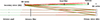 |
Fig. 1. HRIEUV optical design. The HRIEUV channel (Halain et al. 2015) is an off-axis Cassegrain telescope optimized in length and width. The entrance pupils are located at the front section of dedicated entrance baffles and have a diameter of 47.4 mm. |
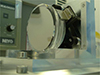 |
Fig. 2. Picture of the HRIEUV primary mirror flight model before integration in the EUI instrument. |
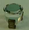 |
Fig. 3. Picture of the HRIEUV secondary mirror flight model before integration in the EUI instrument. |
HRIEUV main telescope and detector requirements.
The solar light enters the instrument through the Solar Orbiter heat shield feedthrough designed to prevent light reflection inside the entrance pupils and to limit the stray light while avoiding additional heat load (see Fig. 3 of Rochus et al. 2020). The reflective entrance baffle rejects more than 60% of the heat coming through the entrance pupil, which is located at the front section of the entrance baffle and has a diameter of 47.4 mm.
The HRIEUV entrance filter (Fig. 4) is located at the end of the front baffle and consists of a 150 nm aluminium thin-foil film supported by custom 20 lines per inch (lpi) nickel patterned mesh, and a rib structure that divides the filter area into sectors to improve thermal conductivity and mechanical resistance. The entrance filter mesh contributes a diffraction pattern to the PSF and the rib structure blocks the incident light by a geometrical factor of 10%. The entrance filter provides protection against excessive heat input on the mirror and efficient rejection of the visible light. An additional filter wheel (Fig. 5), comprising two EUV filters (nominal and redundant, similar to the entrance filter) and open positions, is located at the output pupil in front of the detector. These filters also have a minor effect on the spectral purity of the telescope spectral response, as is shown in Section 4. The entrance and rear EUV filters are of primary importance for the instrument to avoid contamination with visible light that can be 108 times more intense than the EUV flux.
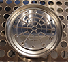 |
Fig. 4. HRIEUV entrance filter. |
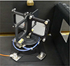 |
Fig. 5. HRIEUV focal plane SN07 and SN10 aluminium filters mounted on the filter wheel. On the right, the cold cup that limits the FoV in the image plane to 2340x2348 pixels. |
The EUV sensitivity of the HRIEUV detector is achieved with backside illumination. The sensor is made of two stitching blocks of 3072 × 1536 pixels of 10 micrometers each, containing a dual-gain pixel architecture (Table 1). The APS sensor and the front-end electronics are located behind a cold cup in front of the detector, which acts as a field stop and limits the light within 2348 × 2340 pixels in the detector plane. The front-end electronics acquire the detector signal with a 14-bit ADC that rounds the signal to 12 bits, separately for the low-gain (LG) and high-gain (HG) read-out. For high-dynamic-range applications, the HG and LG signal are combined on board before compression. Details of the detector can be found in Benmoussa et al. (2013).
A passive thermal control maintains the detector temperature below –50 °C with a stability of ± 2 °C. The camera contains one nominal heater to enable in-flight bake-out and annealing, and two calibration LEDs (Micropac 62162-101, emitting at 470nm) to monitor the detector performance in-flight.
3. Component characterization
The telescope effective response, Reff, in cm2.sr.DN.ph−1 is the product of the telescope throughput with its spectral response, R(λ), and is equal to
 (1)
(1)
where Ageom is the entrance aperture area, equal to ≈15.9 cm2, taking into account the 10% opacity of the rib structure, and δΩ is the pixel platescale, equal to 0.492 arcsec.pixel−1.
The telescope response, R(λ), can be further broken down as the multiplication of the optical efficiency, E(λ), with the detector electronic gain, g(x, y), and detector efficiency, D(x, y, λ):
 (2)
(2)
where x (respectively y) is the column (respectively row) pixel coordinate. The measurements of filters and mirrors that characterize the optical efficiency, E(λ), are discussed in Section 3.1. The measurements of the detector electronic gain, g, and detector efficiency, D, are discussion in Section 3.2. An overview of all component measurements is given in Table 2. Measurements were made on similar reference components rather than on the flight model as detailed in Auchère & team (2013).
Overview of HRIEUV components with their references.
3.1. Filters and mirrors
The overall optical efficiency, E(λ), is given by the formula
 (3)
(3)
where TEF(λ) is the entrance filter transmission, RM1(λ) (respectively RM2(λ)) is the primary (respectively secondary) mirror reflectance, and TFP(λ) is the focal plane filter.
The entrance filter spectral transmittance was measured at PTB/MLS (Berlin, Germany) in the grazing incidence beamline and at the SOLEIL synchrotron (Orsay, France) and is shown in Fig. 6.
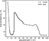 |
Fig. 6. Transmittance of the HRIEUV entrance filter. The dashed line corresponds to the transmittance measured during the characterization campaign. |
The focal filters are mounted on a filter wheel close to the focal plane and in front of the sensor. There are two similar aluminium filters in opposite positions (‘SN07’ and ‘SN10’) and two open positions (see Fig. 5). In the open position, nominal during ground calibration, TFP(λ) = 1. Fig. 16 shows the influence of the aluminium focal plane filters on the telescope response, in particular on the off-band rejection.
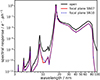 |
Fig. 16. Spectral response, R(λ), simulation using the semi-empirical model of the HRIEUV instrument in the 1 nm–100 nm wavelength range, in electron per incident photon unit. |
The mirror reflectance has been modelled and part of its spectral reflectivity was measured at SOLEIL Synchrotron. The reflectance of the M1 primary mirror (respectively M2) is shown in Fig. 7 (respectively Fig. 8).
 |
Fig. 7. Reflectance of the HRIEUV primary mirror, M1. The plain line part of the curve corresponds to the reflectance measured during the characterization campaign, while the dashed line is the modelled reflectance. |
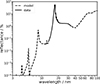 |
Fig. 8. Reflectance of the HRIEUV secondary mirror, M2. The plain line part of the curve corresponds to the reflectance measured during the characterization campaign, while the dashed line is the modelled reflectance. |
3.2. Detector dark current
The detector efficiency, D, expressed in electrons per photon, is defined as the ratio of the number of detected photoelectrons to the number of incident photons, Iph, following the definition of the detected pixel signal, Ie:
 (4)
(4)
where λ is the incident photon wavelength, IDS = Io + IDC Δt is the dark signal, Δt the integration time, Io the electronic offset, T the detector temperature, and ϵrn random readout signal.
During in-flight commissioning, the detector was cooled down to -50 °C. At this temperature, the dark signal was acquired and analysed to estimate the pixel dark current and its spatial variability also called dark-signal non-uniformity. The dark signal acquired at 2 second integration time is shown in Fig. 9, with best detector settings optimized in-flight and optimized 2K × 2K centring.
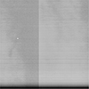 |
Fig. 9. Average dark signal image at 2-s integration time of the HG image acquired in-flight. The signal is dominated by a four-column repeating pattern due to the column gain multiplexing. The read noise is low due to averaging and the dark current is negligible at operating temperature (–50°C). The stitching line of the detector is visible here as a column with an off-point due to the optimized 2K × 2K centring. |
At operational temperature (–50 °C) a dark current inferior to 0.1 e−.s−1.pix−1 was measured (see Fig. 10). The negative values are due to the noise on the estimation of the average dark current values.
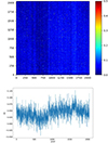 |
Fig. 10. Dark current estimation during in-flight calibration campaigns (March 25, 2021). Top: Dark current image showing the per-pixel dark current estimated using 50-frame on-board average of 10 second integration time images. The colour table indicates the dark current value expressed in electrons per second. Bottom: Per-column average dark current corresponding to detector rows. The dark current values are below 0.1 e−.s−1. The negative values are due to the noise on the estimation of the average dark current values. |
Similarly, the electronic gain, ge, is confirmed using the dark current at +20 °C. The measured signal in DN is the signal at the output of the ADC and equal to IDN(λ) = ge Ie(λ), where ge is the electronic gain and the signal was quantized by the ADC. The electronic gain was measured using the on-board visible LED and mean-variance relationship, similar to the photon transfer curve (PTC) method, and is equal to 0.64 DN.e−1 (spatial mean) in the HG channel.
3.3. Detector spectral response
Using the PTB synchrotron light source, we measured the spatially averaged EUV efficiency of the detector (in both HG and LG) by computing the ratio of detected DNs to incident photons measured by reference detectors at each scanned wavelength between 10 and 40 nm as in
 (5)
(5)
where ΦDN it the detected flux and Φref is the incident EUV photons signal provided by the reference detector.
In order to estimate the signal flux ΦDN, a series of ten images of the beam flux signal for each increasing integration time, Δt, was taken. For each integration time, we computed the temporal mean, μDN, and variance signals, σDN2.
The detected flux was obtained from the signal by fitting
 (6)
(6)
where ϵ is the residual value of the image offset, after removing a dark frame, IDS, at the same integration time, from IDN. Because of the non-uniformity of the beam, the flux was spatially averaged and divided by the indicent flux as measured by reference calibrated detectors. As is explained above, the in-flight measurements show a negligible dark current at typical integration times (≤1 DN/pix for exposures up to 10 s).
The temporal variance of the detected signal, σDN2, relates to the mean signal, μDN, through the ‘mean-variance’ law:
 (7)
(7)
where ge is the electronic gain (number of DN per electron) and g is the EUV effective gain (number of generated electrons per incoming photon), μDN, o is the mean offset, and σϵ2 the readout noise variance. The effective gain, g, also includes the variance in the number of electron-hole charge generation per interacting photon, also known as Fano noise. An average map of μDN, o is shown in Fig. 9.
The signal variance was measured during the detector characterization campaign at the same wavelengths as for the efficiency and the gain was estimated using the mean-variance relationship.
The detector spectral response was measured at PTB in January 2017. Each flight model detector spectral response was measured between 16 nm and 30.4 nm. At each wavelength, a total of ten images was acquired in order to estimate the detector efficiency and effective gain defined hereafter. In order to protect the sensor, the EUV beam was localized in the bottom right side of the image area.
Fig. 11 shows the value of the gain as a function of wavelength, measured and compared to our semi-empirical model-based simulated data. The measured effective gain is systematically lower than the theoretical value given by the quantum-yield-predicted value of a fully depleted detector, in which nearly all electrons can be assumed to be collected in the pixel photodiode.
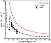 |
Fig. 11. Detector pixel photodiode EUV photon gain of the HRIEUV detector, with measured data overplotted on the simulated data using detector efficiency model. |
The mean signal-to-noise ratio (S/N) is given by
 (8)
(8)
where σDN is given by Eq. (7). The beginning-of-life rms (root-mean-square) readout noise is σϵ = 2.8 e = 1.8 DN, as is shown in Fig. 12. At 17.4 nm, the value of ge g is equal to ≈7 DN.ph−1.
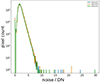 |
Fig. 12. Histogram of HRIEUV read noise. |
3.3.1. Non-linearity
The non-linearity close to pixel well saturation is assessed by acquiring a set of ten LED images at multiple increasing integration times, as is shown in Fig. 13. In the linear part, the signal flux is proportional to the light flux emitted by the LED, while the ‘saturation’ region corresponds to the pixel full well saturation. Because of the non-uniformity of the LED signal, and the limited telemetry, the non-linearity was assessed on re-binned images, and in a region of interest above and close to the stitching line (in the detector reference frame). The non-linearity is clearly reached before the ADC saturation (4095 DN) of the LG channel (see Fig. 14). Non-linearity is measured as a percentage of the linear part of the LG signal in DN, corresponding, respectively, to the 1%, 2%, 5%, and 10% deviation from linear behaviour (see Table 3).
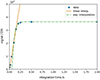 |
Fig. 13. Example of non-linearity estimation of a typical LG pixel exposed with blue 470 nm light (locally averaged using binning for statistical reasons). The LG signal is measured in DN, here shown as a function of integration time, and modelled by an exponential saturation and compared to the linear regression in the linear range of the sensor. |
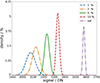 |
Fig. 14. Histogram of pixels for several non-linearity levels, expressed in pixel density in percentage, and measured with on-board LED illuminated LG images. Each curve corresponds to the distribution of pixels at a given non-linearity value, close to saturation, as is indicated by the legend colour. The full well saturation is reached at around 3558 DN, which corresponds to a saturation full well capacity of 131 ke−. |
Detector non-linearity values taken with on-board calibration LED.
The APS detector shows a negligible low-signal non-linearity, in particular at very low integration times. The detector linearity in the HG channel is nearly perfect, while in combined images, at high intensity, the signal becomes non-linear near saturation. The main cause for the detector full well saturation non-linearity resides in the saturation of the pixel LG sense node (or floating diffusion capacitance).
3.3.2. Spatial noise and flat field
Due to a HRIEUV flight detector change, the EUV flat field of the detector could not be measured using EUV light on-ground. We therefore used the nominal calibration LED to estimate the flat field, despite its disadvantages; namely, spatial non-uniformity and stabilization time. Note that since the photon attenuation depth is similar at the operation wavelength (17 nm) and the LED peak wavelength (470 nm), the flat field obtained using the calibration LEDs correlates very well with the EUV flat field. This was confirmed by measurements of EUI/FSI data, which have the same CMOS APS back-side illuminated technology. The flat field in Fig. 15 was thus derived from on-board calibration LED measurements that were averaged and processed on-ground.
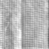 |
Fig. 15. Detector flat field derived from on-board calibration LEDs. The detector stitching line is visible as a column in the image, although it is aligned with the detector rows. This is due to the fact that from level L1, images are rotated by 90 degrees to orient solar north in the upward direction. The regular pattern is caused by the beam of the laser annealing used to activate the shallow p+ implant at detector backside. |
3.4. Telescope spectral response
The multiplication of component performance functions in Eq. (2) gives the simulated the instrument performance shown in Fig. 16.
4. End-to-end calibration
The end-to-end EUV calibration campaign was performed on April 25 2017 at the Metrology Light Source of PTB, Berlin (Germany) with EUI mounted on a dedicated support bracket fixed in a vacuum chamber that connected to the MLS U125 beamline, which had a beam divergence lower than 2 microrad (Gottwald et al. 2019).
After the vacuum pumping of the tank, stabilizing the detector temperature to –35 °C and centring the EUV beam (≈2 mm by 1 mm at the centre of the entrance filter) in the HRIEUV FOV, the first light image Fig. 17 was acquired. After that the beam flux was decreased from the initial 109 ph.s−1 to 106 ph.s−1. For the first part of the measurements, the filter wheel was set in an open position. This allowed us to scan the entrance aperture and confirm its diameter of 47.4 mm. Images were acquired in single-exposure mode, and using the flight model instrument electronics.
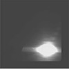 |
Fig. 17. HRIEUV first image acquired during ground calibration. In the bottom right, the occultation of the EUV beam in the detector plane is visible. |
4.1. End-to-end spectral response measurements
The end-to-end telescope response was measured by acquiring ten images of the EUV beam at each wavelength between 16 and 18.5 nm with a 0.1 nm sampling between 17 and 17.6 nm. The target PSF design objectives was to have 90 % of signal energy into one pixel, > 90% PSF energy in 1 pix, < 1 DN scattered light, and < 1 DN ghost images. The three main components of the stray-light signal are the optics PSF, the light reflected off mechanical parts, and the ghost images. During end-to-end calibration, the 17.4 nm high-flux beam was off-pointed at 0.5, 1, and 1.5 degree along the x axis to measure stray light. No significant stray light has been measured.
The HRIEUV high and low effective gains were measured by computing the per-pixel temporal mean and variance of a set of ten images per integration time (Fig. 18). The fitting of the variance as a function of the mean signal, after dark signal correction, for each wavelength, gives the spectral effective gain. Combining several previously discussed results, one arrives at the end-to-end telescope response as shown in Fig. 21 and Fig. 22.
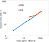 |
Fig. 18. Photon transfer curve (PTC) curves showing the matching of the HG and LG pixel values obtained with EUV light at 17.4 nm. The HG lowest detected signal has a signal sigma of 3 e− rms, which corresponds to its expected readout noise, at the detection limit. Due to the protection measure on the detector, the EUV flux was kept low so the saturation was not reached and no full well saturation is visible. |
Another method of estimating the spatial average of the EUV effective gain at a single wavelength is to take advantage of the EUV beam non-uniformity and fit the scatterplot of pixelwise variance versus signal. This is done for LG and HG in respectively Figs. 19 and 20. All these measurements confirmed a HG effective gain of ≈7 DN.ph−1 at 17.4 nm.
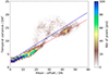 |
Fig. 19. Single integration time image PTC estimation of the LG with EUV beam light. The linear fit (red line) gives a photon to DN LG value of 0.279 DN.ph−1. Pixels located to the pattern above the linear regression blue line undergo the ‘ripple effect’. |
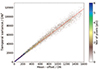 |
Fig. 20. Single integration time image PTC estimation of the high gain with EUV beam light. The robust red linear fit gives a photon to DN HG value of 7.29 DN.ph−1. This corresponds to a gain ratio (HG/LG) of ≈ 26. |
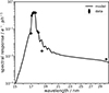 |
Fig. 21. Spectral response of the HRIEUV instrument measured during ground calibration, including the 30.4 nm wavelength measurement, with the filter wheel in open position. |
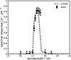 |
Fig. 22. Spectral response of the HRIEUV instrument measured during ground calibration. |
4.2. Expected count rates
With the focal plane filter in the aluminium filter position (SN-10), the expected response corresponding of the emission measure models of a coronal hole, quiet-Sun, an active region, and a flare are given in Table 6. For each region, the expected detected pixel flux, ϕDN, was computed from DEM values as in the following equation:
 (9)
(9)
 (10)
(10)
where the temperature response K(T) (Fig. 23) is the product of R(λ) defined in Eq. 2 and the contribution function G expressed in units ph.cm3.s−1.sr−1, while EM(Ti) is the emission measure at temperature Ti, obtained for an electronic density of Ne= 109 cm−3 using Chianti (Landi et al. 2012; Del Zanna et al. 2021). The median signal flux measured in first light images on May 12 2020 (12:50:14.704 UT) (average L2 signal) is ≈600 DN.s−1, corresponding to the expected quiet Sun signal and within confidence interval.
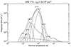 |
Fig. 23. Temperature response of the HRIEUV telescope. |
4.3. Detector artefacts
The HRIEUV detector has deficient pixels and artefacts. A ‘ripple’ effect visible in the LG pixels consists of a signal ‘bump’ and drop at a certain distance of a high signal with which it seems to correlate well. Since this was discovered after focal-plane assembly and just before end-to-end calibration, it could not be well characterized on-ground.
A small area of the detector contains deficient pixels (together know as ‘the jelly baby’) that are highly non-linear. At the edge of the detector (left band in the detector frame), the signal is clipped to zero. A few bad (hot) pixels were identified on-ground.
5. Discussion and conclusion
This paper reviews the initial radiometric calibration of the HRIEUV telescope, obtained from (1) the on-ground characterization of individual components (filters, mirrors, detector), (2) the on-ground end-to-end calibration, and (3) the in-flight commissioning data. The measurements from these three phases together constitute the initial reference for radiometric analysis and monitoring of the telescope in-flight degradation. It is to be noted, however, that, in particular for sensor related parameters, the measurement conditions over the three phases have not been identical.
Relative uncertainty budget of optical components for a coverage factor of k = 2 (2-s uncertainty).
For example, during on-ground measurements, the detector was cooled to the expected operational temperature of –30°C. Once in flight, the measured operational temperature was –50°C. The most impacted parameter is the sensor dark current. Since HRIEUV data users will only be concerned with the actual operational temperature, the quoted dark current in Table 5 is at –50°C. This value is compatible with expectations based on an extrapolation of the earlier values obtained on the ground of –30°C. Moreover the ground characterization at the component level of the EUI flight model detectors was done using the electrical ground support equipment provided by the sensor manufacturer, while the end-to-end calibration and commissioning of the detector used the purpose-built HRIEUV camera and instrument computer. This change can affect parameters such as the electronic gain, linearity, and read-noise. Again, the quoted numbers in Table 5 are the in-flight numbers, which, after straightforward conversions, are compatible with pre-flight expectations. Finally, the EUI sensor is driven by a registry of settings. On ground-measurements of the sensor used the manufacturer values for these settings. In flight we deviated from these settings, in particular settings that control the offset and clipping of the HG and LG read-out, to optimize the on-board reconstruction of HG and LG values into a combined gain range.
HRIEUV telescope measured performance summary.
Expected solar flux for different solar regions.
During the integration of the instrument, the selected flight detector was broken and replaced by the flight spare. Unfortunately no EUV flat field for the flight spare had been determined in the January 2017 campaign at IAS. As a fall-back option it was decided that the on-board ‘blue’ LED would be used, with a peak emission at 470 nm, in order to derive the flat field required by the ground calibration procedure.
Table 5 summarises the overall results obtained that are relevant for HRIEUV observers and data users, and that can serve as a reference for future in-flight monitoring. The pre-flight radiometric calibration of the HRIEUV has confirmed the very high BOL sensitivity of the telescope (> 1.6 electrons per EUV photon at peak wavelength) when compared to the low dark current at operating temperature (< –50 °C) and the low read-out noise (2.8 electrons rms) in the HG mode. The telescope spectral response semi-empirical model is validated by the pre-flight end-to-end ground calibration of the instrument with an uncertainty of 17% for the end-to-end optical efficiency. HRIEUV Level 2 images1 were calibrated using the euiprep2 Python routine that was built upon the calibration measurements presented in this paper. The euiprep repository also includes the numerical values for the spectral and thermal response functions.
The expected mission lifetime of Solar Orbiter, and thus of EUI and HRIEUV, is of the order of 10 years, and degradation of the telescope sensitivity over the long term can be expected (Sandford et al. 2025). A programme of continuous monitoring of the performance evolution has therefore been put in place: dark and LED images are taken on a monthly basis and their brightness and ratios are studied as a function of time (Dickson 2025). Upcoming analysis will incorporate the results of this program in the calibration software used to produce the EUI science data products.
Acknowledgments
Solar Orbiter is a space mission of international collaboration between ESA and NASA, operated by ESA. The EUI instrument was conceived by a multi-national consortium and proposed in 2008 under the scientific lead of Royal Observatory of Belgium (ROB) and the engineering lead of Centre Spatial de Liège (CSL) and built by CSL, IAS, MPS, MSSL/UCL, PMOD/WRC, ROB, LCF/IO with funding from the Belgian Federal Science Policy Office (BELSPO/PRODEX PEA C4000134088. DML is grateful to the Science Technology and Facilities Council for the award of an Ernest Rutherford Fellowship (ST/R003246/1).
References
- Auchère, F., & team, E. 2013, in EUI Science and Instrument Requirement Document SP-IAS-SOEUI-11092, Tech. rep., IAS [Google Scholar]
- Benmoussa, A., Giordanengo, B., Gissot, S., et al. 2013, IEEE J. Electron Dev., 60, 1701 [Google Scholar]
- BenMoussa, A., Gissot, S., Giordanengo, B., et al. 2013, IEEE Trans. Nucl. Sci., 60, 3907 [Google Scholar]
- Berghmans, D., Antolin, P., Auchère, F., et al. 2023, A&A, 675, A110 [NASA ADS] [CrossRef] [EDP Sciences] [Google Scholar]
- Boerner, P., Edwards, C., Lemen, J., et al. 2011, Sol. Phys., 275, 41 [Google Scholar]
- Del Zanna, G., Dere, K. P., Young, P. R., & Landi, E. 2021, ApJ, 909, 38 [NASA ADS] [CrossRef] [Google Scholar]
- Delaboudinière, J. P., Artzner, G. E., Brunaud, J., et al. 1995, Sol. Phys., 162, 291 [Google Scholar]
- Delmotte, F., Meltchakov, E., de Rossi, S., et al. 2013, SPIE, 8862, 88620A [Google Scholar]
- Dere, K., Moses, J., Delaboudinière, J. P., et al. 2000, Sol. Phys., 195, 13 [Google Scholar]
- Dickson, E. C. M. 2025, in EUI Sensor Monitoring Plots (Royal Observatory of Belgium (ROB)), https://www.sidc.be/EUI/data/calibration/ [Google Scholar]
- Gottwald, A., Kroth, U., Richter, M., Schöppe, H., & Ulm, G. 2010, Measurement. Sci. Technol., 21, 125101 [Google Scholar]
- Gottwald, A., Kaser, H., & Kolbe, M. 2019, J. Synchrotron Rad., 26, 535 [Google Scholar]
- Halain, J.-P., Berghmans, D., Seaton, D. B., et al. 2012, Sol. Phys., 286, 67 [Google Scholar]
- Halain, J.-P., Rochus, P., Renotte, E., et al. 2014, SPIE, 9144, 914408 [Google Scholar]
- Halain, J.-P., Mazzoli, A., Meining, S., et al. 2015, in SPIE Proceedings, eds. S. Fineschi, & J. Fennelly [Google Scholar]
- Handy, B., Acton, L., Kankelborg, C., et al. 1999, Sol. Phys., 187, 229 [Google Scholar]
- Kobayashi, K., Cirtain, J., Winebarger, A. R., et al. 2014, Sol. Phys., 289, 4393 [Google Scholar]
- Landi, E., Del Zanna, G., Young, P. R., Dere, K. P., & Mason, H. E. 2012, ApJ, 744, 99 [Google Scholar]
- Lemen, J. R., Title, A. M., Akin, D. J., et al. 2011, Sol. Phys., 275, 17 [Google Scholar]
- Rachmeler, L. A., Winebarger, A. R., Savage, S. L., et al. 2019, Sol. Phys., 294, 174 [Google Scholar]
- Rochus, P., Aucheère, F., Berghmans, D., et al. 2020, A&A, 642, A8 [NASA ADS] [CrossRef] [EDP Sciences] [Google Scholar]
- Sandford, E., Auchère, F., Mortier, A., Hayes, L. A., & Müller, D. 2025, A&A, 699, A353 [NASA ADS] [CrossRef] [EDP Sciences] [Google Scholar]
- Seaton, D. B., Berghmans, D., Nicula, B., et al. 2012, Sol. Phys., 286, 43 [Google Scholar]
- Wülser, J.-P., Lemen, J. R., & Nitta, N. 2007, SPIE Proc., 6689, 668905 [Google Scholar]
All Tables
Relative uncertainty budget of optical components for a coverage factor of k = 2 (2-s uncertainty).
All Figures
|
Fig. 1. HRIEUV optical design. The HRIEUV channel (Halain et al. 2015) is an off-axis Cassegrain telescope optimized in length and width. The entrance pupils are located at the front section of dedicated entrance baffles and have a diameter of 47.4 mm. |
| In the text | |
|
Fig. 2. Picture of the HRIEUV primary mirror flight model before integration in the EUI instrument. |
| In the text | |
|
Fig. 3. Picture of the HRIEUV secondary mirror flight model before integration in the EUI instrument. |
| In the text | |
|
Fig. 4. HRIEUV entrance filter. |
| In the text | |
|
Fig. 5. HRIEUV focal plane SN07 and SN10 aluminium filters mounted on the filter wheel. On the right, the cold cup that limits the FoV in the image plane to 2340x2348 pixels. |
| In the text | |
|
Fig. 6. Transmittance of the HRIEUV entrance filter. The dashed line corresponds to the transmittance measured during the characterization campaign. |
| In the text | |
|
Fig. 16. Spectral response, R(λ), simulation using the semi-empirical model of the HRIEUV instrument in the 1 nm–100 nm wavelength range, in electron per incident photon unit. |
| In the text | |
|
Fig. 7. Reflectance of the HRIEUV primary mirror, M1. The plain line part of the curve corresponds to the reflectance measured during the characterization campaign, while the dashed line is the modelled reflectance. |
| In the text | |
|
Fig. 8. Reflectance of the HRIEUV secondary mirror, M2. The plain line part of the curve corresponds to the reflectance measured during the characterization campaign, while the dashed line is the modelled reflectance. |
| In the text | |
|
Fig. 9. Average dark signal image at 2-s integration time of the HG image acquired in-flight. The signal is dominated by a four-column repeating pattern due to the column gain multiplexing. The read noise is low due to averaging and the dark current is negligible at operating temperature (–50°C). The stitching line of the detector is visible here as a column with an off-point due to the optimized 2K × 2K centring. |
| In the text | |
|
Fig. 10. Dark current estimation during in-flight calibration campaigns (March 25, 2021). Top: Dark current image showing the per-pixel dark current estimated using 50-frame on-board average of 10 second integration time images. The colour table indicates the dark current value expressed in electrons per second. Bottom: Per-column average dark current corresponding to detector rows. The dark current values are below 0.1 e−.s−1. The negative values are due to the noise on the estimation of the average dark current values. |
| In the text | |
|
Fig. 11. Detector pixel photodiode EUV photon gain of the HRIEUV detector, with measured data overplotted on the simulated data using detector efficiency model. |
| In the text | |
|
Fig. 12. Histogram of HRIEUV read noise. |
| In the text | |
|
Fig. 13. Example of non-linearity estimation of a typical LG pixel exposed with blue 470 nm light (locally averaged using binning for statistical reasons). The LG signal is measured in DN, here shown as a function of integration time, and modelled by an exponential saturation and compared to the linear regression in the linear range of the sensor. |
| In the text | |
|
Fig. 14. Histogram of pixels for several non-linearity levels, expressed in pixel density in percentage, and measured with on-board LED illuminated LG images. Each curve corresponds to the distribution of pixels at a given non-linearity value, close to saturation, as is indicated by the legend colour. The full well saturation is reached at around 3558 DN, which corresponds to a saturation full well capacity of 131 ke−. |
| In the text | |
|
Fig. 15. Detector flat field derived from on-board calibration LEDs. The detector stitching line is visible as a column in the image, although it is aligned with the detector rows. This is due to the fact that from level L1, images are rotated by 90 degrees to orient solar north in the upward direction. The regular pattern is caused by the beam of the laser annealing used to activate the shallow p+ implant at detector backside. |
| In the text | |
|
Fig. 17. HRIEUV first image acquired during ground calibration. In the bottom right, the occultation of the EUV beam in the detector plane is visible. |
| In the text | |
|
Fig. 18. Photon transfer curve (PTC) curves showing the matching of the HG and LG pixel values obtained with EUV light at 17.4 nm. The HG lowest detected signal has a signal sigma of 3 e− rms, which corresponds to its expected readout noise, at the detection limit. Due to the protection measure on the detector, the EUV flux was kept low so the saturation was not reached and no full well saturation is visible. |
| In the text | |
|
Fig. 19. Single integration time image PTC estimation of the LG with EUV beam light. The linear fit (red line) gives a photon to DN LG value of 0.279 DN.ph−1. Pixels located to the pattern above the linear regression blue line undergo the ‘ripple effect’. |
| In the text | |
|
Fig. 20. Single integration time image PTC estimation of the high gain with EUV beam light. The robust red linear fit gives a photon to DN HG value of 7.29 DN.ph−1. This corresponds to a gain ratio (HG/LG) of ≈ 26. |
| In the text | |
|
Fig. 21. Spectral response of the HRIEUV instrument measured during ground calibration, including the 30.4 nm wavelength measurement, with the filter wheel in open position. |
| In the text | |
|
Fig. 22. Spectral response of the HRIEUV instrument measured during ground calibration. |
| In the text | |
|
Fig. 23. Temperature response of the HRIEUV telescope. |
| In the text | |
Current usage metrics show cumulative count of Article Views (full-text article views including HTML views, PDF and ePub downloads, according to the available data) and Abstracts Views on Vision4Press platform.
Data correspond to usage on the plateform after 2015. The current usage metrics is available 48-96 hours after online publication and is updated daily on week days.
Initial download of the metrics may take a while.