| Issue |
A&A
Volume 706, February 2026
|
|
|---|---|---|
| Article Number | A229 | |
| Number of page(s) | 19 | |
| Section | Numerical methods and codes | |
| DOI | https://doi.org/10.1051/0004-6361/202452669 | |
| Published online | 19 February 2026 | |
Bayesian multiband imaging of SN1987A in the Large Magellanic Cloud with SRG/eROSITA
1
Max Planck Institute for Astrophysics,
Karl-Schwarzschild-Straße 1,
85748
Garching,
Germany
2
Ludwig-Maximilians-Universität München,
Geschwister-Scholl-Platz 1,
80539
Munich,
Germany
3
Kavli Institute for Particle Astrophysics & Cosmology, Stanford University,
Stanford,
CA
94305,
USA
4
Max Planck Institute for Extraterrestrial Physics,
Gießenbachstraße 1,
85748
Garching,
Germany
5
Excellence Cluster ORIGINS,
Boltzmannstraße 2,
85748
Garching,
Germany
★★ Corresponding authors: This email address is being protected from spambots. You need JavaScript enabled to view it.
; This email address is being protected from spambots. You need JavaScript enabled to view it.
; This email address is being protected from spambots. You need JavaScript enabled to view it.
Received:
18
October
2024
Accepted:
27
September
2025
Abstract
The eROSITA Early Data Release (EDR) and eROSITA All-Sky Survey (eRASS1) data have already revealed a remarkable number of undiscovered X-ray sources. Using Bayesian inference and generative modeling techniques for X-ray imaging, we aim to increase the sensitivity and scientific value of these observations by denoising, deconvolving, and decomposing the X-ray sky. Leveraging information field theory, we can exploit the spatial and spectral correlation structures of the different physical components of the sky with non-parametric priors to enhance the image reconstruction. By incorporating instrumental effects into the forward model, we developed a comprehensive Bayesian imaging algorithm for eROSITA pointing observations. Finally, we applied the developed algorithm to EDR data of the Large Magellanic Cloud (LMC) SN1987A, fusing datasets from observations made by five different telescope modules. The final result is a denoised, deconvolved, and decomposed view of the LMC, which enables the analysis of its fine-scale structures, the identification of point sources in this region, and enhanced calibration for future work.
Key words: methods: data analysis / techniques: image processing / ISM: general / X-rays: general
These authors contributed equally to this work.
© The Authors 2026
 Open Access article, published by EDP Sciences, under the terms of the Creative Commons Attribution License (https://creativecommons.org/licenses/by/4.0), which permits unrestricted use, distribution, and reproduction in any medium, provided the original work is properly cited.
This article is published in open access under the Subscribe to Open model.
Open Access funding provided by Max Planck Society.
1 Introduction
The eROSITA X-ray Telescope (Predehl et al. 2021) on Spectrum-Roentgen-Gamma (SRG) (Sunyaev, R. et al. 2021) was launched on July 13, 2019, from the Baikonour Cosmodrome. Since the full-sky survey of ROSAT (Truemper 1982) in 1990, eROSITA is the first X-ray observatory to perform a fullsky survey with higher resolution and a larger effective area. After a Calibration and Performance Verification (CalPV) phase of pointed and field-scan observations, the main phase of the mission has been devoted to multiple all-sky surveys of the celestial sphere, each lasting about 6 months. The amount of data collected by the X-ray observatory in its about 4.3 completed all-sky surveys has already had a huge scientific impact. In order to make use of its scientific data, nuisance effects of the instrument need to be understood and removed whenever possible. Amongst others, Poisson noise and the point spread function (PSF) of the optical system cause problems to source detection algorithms. Unfortunately, some of these effects are not analytically invertible and thus leave us with an ill-posed problem at hand. In this work, we make use of information field theory (IFT) (Enßlin et al. 2009) as a theoretical framework to tackle these problems. The use of prior knowledge and generative modeling enables us to remove instrumental effects, decompose the sky into astrophysical emission components, and potentially remove the high-energy particle background, leaving us with an approximation of the posterior distribution. This permits us to gain knowledge about any posterior measure of interest, such as the mean and the uncertainty of the measured physical quantities.
X-ray astronomy has developed rapidly since its beginnings in the 1960s, driven by major X-ray missions such as Einstein and ROSAT. This rapid progress has been fueled not only by advancements in instrumentation, with ever-improving telescopes such as Chandra (Garmire et al. 2003), XMM-Newton (Schartel & Dahlem 2000), and more recently eROSITA, but also by simultaneous developments in imaging techniques. These advancements have steadily increased the amount of information extracted from observations and enabled researchers to address various data-analysis challenges. For instance, tasks such as source detection and the coherent fusion of overlapping datasets – some of the most difficult tasks in astrophysical imaging – along with the denoising and deconvolution of X-ray data affected by Poisson noise, have become more manageable due to these innovations.
In Westerkamp et al. (2024), an overview of general source detection algorithms is given, such as the sliding cell algorithm (Calderwood et al. 2001), the wavelet detection algorithm (Freeman et al. 2002), and the Voronoi tessellation and percolation algorithm (Ebeling & Wiedenmann 1993), as well as an overview on data fusion techniques currently used and implemented for Chandra data. A summary of the data processing and imaging pipelines for the Chandra and XMM-Newton X- ray telescopes is available at Seward & Charles (2010). This section provides an overview of the state of the art in X-ray imaging techniques specifically for eROSITA. For eROSITA data analysis, there is the eROSITA Science Analysis Software System (eSASS) (Brunner et al. 2018; Merloni et al. 2024), which includes all the functionalities of the standard eROSITA processing pipeline, such as event processing, event file and image generation, background estimation and point source detection, and source-specific output such as light curve and spectrum generation. In Brunner et al. (2022), the standard eROSITA source detection pipeline using eSASS for the eROSITA Final Equatorial-Depth Survey (eFEDS) is elaborated step by step. First, the standard source detection requires a preliminary source list containing all possible source candidates, which is generated using the sliding cell algorithm. Based on the preliminary source catalog, the X-ray data are compared to a PSF model using maximum likelihood fitting. Finally, as noted in Merloni et al. (2024), circular regions of appropriate radius can be placed around point sources to exclude them, thereby obtaining point-source-subtracted images. All the necessary functionalities, including the sliding cell algorithm, are implemented in the corresponding eSASS package. To test the completeness and accuracy of this source detection pipeline, Liu et al. (2022) simulated eFEDS data, given a specific catalog and background, and applied the source detection algorithm to it. Seppi et al. (2022) also estimated the fraction of spurious sources for eROSITA All-Sky Survey (eRASS1) using the eSASS pipeline in different configurations.
Recently, Merloni et al. (2024) published a catalog of point sources and extended sources in the western Galactic hemisphere using the first of the all-sky scans of eRASS1. In this study, we focus on the imaging of the Large Magellanic Cloud (LMC) using eROSITA Early Data Release (EDR) data from the CalPV phase. As the nearest star-forming galaxy, the LMC has already been observed and analyzed in its various parts across the entire electromagnetic spectrum, as noted in Zangrandi et al. (2024); Zanardo et al. (2013). Among other things, the numerous supernova remnants (SNRs) present in it are of interest, as studied in Zangrandi et al. (2024) on data from eRASS:4, including all data from the eROSITA all-sky surveys eRASS1-4. To enhance the edges of the shocked gas in the SNRs, they used the Gaussian gradient magnitude (GGM) filter (Sanders et al. 2016), resulting in 78 SNRs and 45 candidates in the LMC. The most famous supernova (SN) in the LMC is SN1987A, as the only nearby core-collapse SN. SN1987A provides a perfect opportunity to study the evolution of young Type II SNe into the SNR stage. It has therefore been the subject of several publications and observed by several instruments, including ATCA (Zanardo et al. 2013), XMM-Newton (Haberl et al. 2006), Chandra (Burrows et al. 2000), and recently JWST (Matsuura et al. 2024).
In this study, we focus on Bayesian imaging methods for X-ray astronomy based on the algorithm D3PO (Selig & Enßlin 2015), which implements denoising, deconvolution, and decomposition of count data. Decomposition means that, in addition to the total photon flux, the composition of the flux at each pixel is reconstructed using assumptions about prior statistics. The algorithm has been extended by Pumpe et al. (2018) to reconstruct and decompose multi-domain knowledge. The developed algorithm has been applied to Fermi data to reconstruct the spatio-spectral gamma-ray sky in Scheel-Platz et al. (2023), and its capabilities have been shown on X-ray photon-count data for Chandra in Westerkamp et al. (2024). Here, we build a novel likelihood model for the eROSITA instrument and advance the prior model for the X-ray sky to reconstruct LMC features from EDR eROSITA data, as shown below. Moreover, we used variational inference (VI) to approximate the posterior instead of the maximum a posteriori (MAP) approach followed in Pumpe et al. (2018).
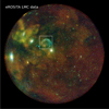 |
Fig. 1 Visualization of the exposure-corrected eROSITA EDR TM8 data of ObsID 700161 for three energy bins. Red: 0.2–1.0 keV, green: 1.0–2.0 keV, blue: 2.0–4.5 keV. The white box marks the region of 30 Doradus C further discussed in Sect. 3.2. The bright central point-like source underneath the bottom-right corner of the 30 Doradus C box is SN1987A. |
2 Observations
We employed observations from the EDR of the LMC SN1987A containing data from the CalPV phase of eROSITA. We used data of the LMC SN1987A from eROSITA in pointing mode with the observation ID 7001611. In total, this observation of the LMC includes all seven telescope modules (TMs) of eROSITA. However, we choose only to use data from five of these TMs, specifically TM1, TM2, TM3, TM4, and TM6 (together usually referred to as TM8), since TM5 and TM7, as noted in Merloni et al. (2024), do not have an on-chip optical blocking filter and suffer from an optical light leak (Predehl et al. 2021). The raw data were processed using the eSASS pipeline (Brunner et al. 2022) and binned into 1024 × 1024 spatial bins and three energy bins, 0.2–1.0 keV (red), 1.0–2.0 keV (green), and 2.0–4.5 keV (blue), according to the binning used by Haberl et al.2.
In particular, we used evtool to generate the cleaned event files and expmap to generate the corresponding exposure maps for each TM. The specific configurations for evtool and expmap can be found in the Appendix A. We created new detector maps that included the bad pixels in order to exclude those from the inference. Figure 1 shows the corresponding RGB image of the eROSITA LMC data, where one image pixel corresponds to four arc seconds. In the appendix in Fig. A.1, the data per energy bin and TM are shown. Figure A.2 shows the exposures summed over the TMs.
3 Methods
In this section, we present the methods used for X-ray imaging with eROSITA. In the end we want to reconstruct a signal s, in our case the X-ray photon flux density field in units of [1/(arcsec2 × s)]3. The signal is described by a physical field and is a function of spatial coordinates, x ∈ ℝ2, and a spectral coordinates, y = log(ℇ/ℇ0) ∈ ℝ, where ℇ is the energy and ℇ0 the reference energy. In the following, we describe the Bayesian inference of the signal field and its components, in other words the prior and the likelihood model.
3.1 Imaging with information field theory
X-ray imaging poses a series of different challenges. Astrophysical sources emit photons at a certain rate. This rate can be mathematically modeled by a scalar field that varies across the field of view (FOV), energy, and time. After being bent through the instrument’s optics, this radiation is then collected by the charge coupled devices (CCDs), which records individual photon counts as events. This way, the physical information contained in the sources’ flux spatio-spectro-temporal distribution is degraded into the observational data. The mathematical object of a field with an infinite number of degrees of freedom, which is well suited to describe the original flux-rate signal, is not suited to describe a finite collection of event counts. Recovering the infinite degrees of freedom of the signal field from finite data is a challenging problem that requires additional information. IFT (Enßlin et al. 2009; Enßlin 2019) provides a mathematical framework to introduce these additional components and solve the inverse problem of recovering fields from data. The additional information introduced characterizes typical source types found in astrophysical observations, such as point sources, which can be bright but are spatially sparse; diffuse emission, which is nearly ubiquitous across the FOV and spatially correlated; and extended sources, which are finite regions of diffuse emission with their own specific correlation structures. In the context of X-ray imaging, this allows accurate and robust reconstruction of the underlying photon flux field as the sum of all modeled emission fields. In essence, upon denoting the quantity of interest, in our case the X-ray flux, with s for signal, we can use prior information on the distribution of s, 𝒫(s), to obtain posterior information 𝒫;(s|d) on the signal constrained to the observed data d using Bayes’ theorem
 (1)
(1)
Here, 𝒫(d|s) is called the likelihood and incorporates information about the instrument’s response and noise statistics, while 𝒫(d) is called the evidence and ensures proper normalization of the posterior 𝒫(s|d). In the following, we discuss our choices for the prior distribution Sect. 3.2), describe how to build the likelihood model which takes into account eROSITA-specific instrumental effects Sect. 3.3), and explain how to combine our likelihood and prior models to numerically approximate the posterior distribution as this turns out to be analytically intractable Sect. 3.4). The corresponding models are built using the software package J-UBIK Eberle et al. 2024), the JAX- accelerated universal Bayesian imaging kit, which is based on NIFTy.re Edenhofer et al. 2024) as a JAX-accelerated version of NIFTy Selig et al. 2013; Arras et al. 2019). Although we focus on eROSITA imaging in this work, the presented algorithm is general and applicable to other photon-count observatories. For instance, in Westerkamp et al. 2024), a similar technique is applied to Chandra data. As instrument models are made publicly available through J-UBIK, with plans to expand the included instruments in the future, this framework enables accurate, high-resolution imaging and has the potential to support multi-messenger imaging.
3.2 Prior models
Prior models are an essential part of Bayesian inference, allowing us to infer a field with a virtually infinite number of degrees of freedom from a finite number of data points. Here we explain how we mathematically model different sky components, their underlying assumptions and justifications, and how these models are implemented in a generative way.
Our signal, s, is composed of a set of sky components, {si},
 (2)
that differ in their morphology. In this study, these are in particular the point source emission, sp, and the diffuse extended source emission, sd. Building individual prior models for each of these components allowed us to decompose the reconstructed, denoised and deconvolved sky into its various sources. The prior models for each of the sky components are implemented as generative models as introduced in Knollmüller & Enßlin (2020) using the reparametrization trick of Kingma et al. (2015). In other words, each of the prior models is described by a set of normal or log-normal models, leading to the final generative model defined via Gaussian processes via inverse transform sampling. In this study, we distinguish between spatially correlated sources, which describe diffuse emission, and spatially uncorrelated sources, which model point sources. For each of the components we have a correlated spectral direction.
(2)
that differ in their morphology. In this study, these are in particular the point source emission, sp, and the diffuse extended source emission, sd. Building individual prior models for each of these components allowed us to decompose the reconstructed, denoised and deconvolved sky into its various sources. The prior models for each of the sky components are implemented as generative models as introduced in Knollmüller & Enßlin (2020) using the reparametrization trick of Kingma et al. (2015). In other words, each of the prior models is described by a set of normal or log-normal models, leading to the final generative model defined via Gaussian processes via inverse transform sampling. In this study, we distinguish between spatially correlated sources, which describe diffuse emission, and spatially uncorrelated sources, which model point sources. For each of the components we have a correlated spectral direction.
There are several ways to implement the correlation in the spatial or spectral dimension. To model the two-dimensional spatial correlation in diffuse emission, we use the correlated field model introduced in Arras et al. (2022). In this particular case the two-dimensional field, which we call φln = eτ, is modelled by a log-normal process with τ being normal distributed, ;(τ|T) = 𝒩;(τ, T), with unknown covariance T,
 (3)
where we denote the Gaussian distribution for a random variable x with covariance X as
(3)
where we denote the Gaussian distribution for a random variable x with covariance X as
 (4)
(4)
Assuming a-priori statistical homogeneity and isotropy, the correlation structure encoded in T can be represented by its power spectrum according to the Wiener–Khinchin theorem. In order to learn the power spectrum and thus the correlation structure simultaneously with the diffuse sky realization, it is implemented by an integrated Wiener process whose parameters are themselves represented by log-normal and Gaussian processes and can thus be learned from the data. For more details on the correlated field model see Arras et al. (2022).
For the point sources, we want the two-dimensional spatial field, φig, to be pixel-wise uncorrelated, or in other words we want each pixel to be independent. Statistically this is described by a probability distribution, which factorizes in spatial direction. Moreover, we aim for a few bright point sources. As shown in Guglielmetti et al. (2009), an appropriate probability distribution is the inverse gamma distribution, i.e.,
 (5)
(5)
As we aim to perform a spatio-spectral reconstruction of the eROSITA X-ray sky, we add a spectral axis. In this study we consider a power-law behavior, described by the spectral index α in spectral direction. For the diffuse emission we assume that the spectral index, αd, is spatially correlated, while it is assumed to be spatially uncorrelated for the point source emission αp. This leads to the mathematical definition of the individual components, sp and sd;
 (6)
(6)
In Fig. 1 it can be seen that both the correlation structure and the spectral power law behavior in the region of 30 Doradus C are fundamentally different from the diffuse structures that are otherwise present in the data. For the diffuse structures in the LMC we expect long correlation structures and a steep powerlaw slope in the energy direction. 30 Doradus C, on the other hand, has a flat power-law and a shorter correlation length. To account for this, we add another prior component, sb, in the region of a box, b, around 30 Doradus C, which has a correspondingly flatter power law and allows for smaller structures, giving us a third component,
 (7)
(7)
The prior model does not take temporal variation into account and thus assumes time invariant flux. Fig. 2 shows one prior sample drawn from the here described prior model for three energy bins. In the Appendix C, we explain how to choose the latent parameters of this generative model in order to find a reasonable prior.
 |
Fig. 2 Visualization of one prior sample drawn from the prior model described in Sect. 3.2 for three energy bins in [1/(arcsec2 × s)]. |
3.3 The likelihood
The likelihood is the conditional probability of a data realization d given the underlying physical signal s. In the case of photoncount instruments like eROSITA, this conditional probability for a pixel i, takes the form of a Poisson distribution,
 (8)
with di being the photon counts and λi being the mean photon flux on the detector pixel i, caused by the signal s. For a CCD chip with n instrument pixels, the data is a vector of pixel photon counts, d = (di)i∈{1,…,n}. The total likelihood turns into the product of the individual likelihoods in the case of statistical independence of the pixel events,
(8)
with di being the photon counts and λi being the mean photon flux on the detector pixel i, caused by the signal s. For a CCD chip with n instrument pixels, the data is a vector of pixel photon counts, d = (di)i∈{1,…,n}. The total likelihood turns into the product of the individual likelihoods in the case of statistical independence of the pixel events,
 (9)
(9)
Often we refer to the negative logarithm of this probability as the information Hamiltonian of the likelihood,
 (10)
(10)
These equations can be generalized to multiple observations m of the same sky with different instruments or at different times. Then the data is a vector of vectors, d = (dj)j∈{1,…m} = (dji)j∈{1,…m}, i∈{1,…,n}, where dji is the data point from the pixel i in the observation j which turns Eq. (10) into
 (11)
(11)
The steps performed to bin the data before using it in this formula are explained in Sect. 2. In order to evaluate the Hamiltonian ℋ;(d|s) we need a digital representation of the measurement process, the relation between the physical signal s, and the expected number of counts λ. The derivation of these quantities is discussed in the following section (Sect. 3.3.1).
3.3.1 Instrument model
An accurate description of the measurement process is essential for the inference of the signal s. Therefore, we need the instrument response R, which represents the effects of the measurement process,
 (12)
to be as accurate as possible. However, since this function is called many times during the computation process, it also has to be efficient, and therefore we aim for a representation that is not only precise but also computationally affordable. In essence, we want to build a forward model that describes the linear effects of the measurement process. We tackle this by subdividing the response function R into its most relevant constituents. The photon flux s coming from the sky gets smeared out by the PSF of the mirror assembly (MA). This gets mathematically described by operator O. The PSF of each individual mirror module onground, on-axis and in-focus is of the order of 16.1 arcsec. However, the modules are mounted intra-focal to reduce the off- axis blurring for the price of an enlarged PSF in the on-axis region. Therefore, the in-flight on-axis PSF is approximately 18 arcsec, and the averaged angular resolution of the field of view is improved to approximately 26 arcsec (Predehl et al. 2021). The blurred flux gets then collected by the camera assembly (CA). We denote the mathematical operator representing the exposure with E. It encodes the observation time and detector sensitivity effects. The flagging of invalid detector pixels, also called the mask, is denoted with M. The instrument response is thus
(12)
to be as accurate as possible. However, since this function is called many times during the computation process, it also has to be efficient, and therefore we aim for a representation that is not only precise but also computationally affordable. In essence, we want to build a forward model that describes the linear effects of the measurement process. We tackle this by subdividing the response function R into its most relevant constituents. The photon flux s coming from the sky gets smeared out by the PSF of the mirror assembly (MA). This gets mathematically described by operator O. The PSF of each individual mirror module onground, on-axis and in-focus is of the order of 16.1 arcsec. However, the modules are mounted intra-focal to reduce the off- axis blurring for the price of an enlarged PSF in the on-axis region. Therefore, the in-flight on-axis PSF is approximately 18 arcsec, and the averaged angular resolution of the field of view is improved to approximately 26 arcsec (Predehl et al. 2021). The blurred flux gets then collected by the camera assembly (CA). We denote the mathematical operator representing the exposure with E. It encodes the observation time and detector sensitivity effects. The flagging of invalid detector pixels, also called the mask, is denoted with M. The instrument response is thus
 (13)
where ◦ denotes the composition of operators. Readout streaks are almost completely suppressed due to the fast shift from the imaging to the frame-store area of the CCDs and therefore, do not have to be modeled (Predehl et al. 2021). Other effects, like pile-up are neglected up to this moment, and deferred to future work. In the following sections, the parts of the instrument response are discussed individually.
(13)
where ◦ denotes the composition of operators. Readout streaks are almost completely suppressed due to the fast shift from the imaging to the frame-store area of the CCDs and therefore, do not have to be modeled (Predehl et al. 2021). Other effects, like pile-up are neglected up to this moment, and deferred to future work. In the following sections, the parts of the instrument response are discussed individually.
3.3.2 The point spread function
The PSF, here denoted as the mathematical operator O, describes the response of the instrument to a point-like source. An incoming photon from direction x ∈ ℝ2 is deflected to a different direction  . This blurs the original incident flux s to the blurred flux s′, which is notated in a continuous and discretized way,
 (14)
(14)
This operator  can be regarded as a probability density function
  , which is normalized by the integration over the space of all directions meaning, that the process of blurring conserves the photon flux,
 (15)
(15)
In the discretized form the operator O is a matrix and thus scales quadratically with the number of pixels n, resulting in a computational complexity of ;(n2). In most applications, a spatially invariant PSF is assumed, meaning that the PSF is the same for all points within the field of view. Thus the PSF is only a function of the deflection  , meaning
  . This fact turns Eq. (14) into a convolution,
 (16)
(16)
Convolutions on regular grids can be executed very efficiently, thanks to the convolution theorem and the fast Fourier transform (FFT) developed by Cooley & Tukey (1965). However, the assumption of spatial invariance of the PSF only holds, depending on the variability of the PSF, for smaller fields of view. To image large structures in the sky, the spatial variability of the PSF cannot be ignored without imprinting artifacts on the reconstructions.
Therefore, we need a representation of spatially variant PSFs that can be used in the forward model. Here, we use the algorithm of Nagy & O'Leary (1997). This algorithm, which we call linear patched convolution in the following, is a method to approximate spatially variant PSFs in a computationally efficient way. It scales sub-quadratically, meaning it is computationally afforable, but improves the accuracy, in comparison to a regular spatially in-variant convolution.
In linear patched convolution, the full spatially variant PSF, O, is approximated by a combination of operations,
 (17)
(17)
First, the image is cut into k overlapping patches by the slicing operator Ck. Next, these patches are weighted with a linear interpolation kernel W, such that the total flux s, despite the overlapping patches, is conserved. Then, each patch is convolved with the associated PSF corresponding to the center of the patch, denoted by Pk. Finally, the results of the weighted and convolved overlapping patches are summed up. This can be seen as an Overlap-Add convolution with linear interpolation and different PSFs for each patch (see Nagy & O'Leary 1997).
In order to perform this operation, we need information about the spatial variability of the PSF across the FOV, which we can retrieve from the calibration database (CALDB)4. Here, we find information about the PSF, gathered at the PANTER 130 meter long-beam X-ray experimental facility of the Max-Planck-Institute for Extraterrestrial Physics (Predehl et al. 2021)5. The CALDB files contain the measurements of the PSF for certain off-axis angles and energies, averaged over the azimuth angle.
For the linear patched convolution algorithm at use we need the PSF at the central positions in the patches. To obtain these, we rotated and linearly interpolated the PSFs from the CALDB, which allowed us to construct the PSFs at these central positions. We also remove some noticeable shot noise from the measured PSFs by clipping the normalized PSFs at 10−6. A visualization of the approximated PSF of eROSITA can be seen in Fig. 3. More detailed information on the eROSITA PSF can be found in Predehl et al. (2021).
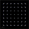 |
Fig. 3 Visualization of eROSITA PSF approximated by the linear patch convolution algorithm for three energy bins. The different colors represent the logarithmic intensities in the three energy bands. Red: 0.2–1.0 keV, green: 1.0–2.0 keV, blue: 2.0–4.5 keV. |
3.3.3 The exposure
The received flux λ on the camera is observed for a total exposure time Θ by the CA. The exposure operator E includes not only the exposure time Θ, but also the vignetting, ρ, of the TM, and its effective area μ. In the case of a time-invariant flux  , the integral over time corresponds to a multiplication with the total exposure time Θ, and thus
 (18)
(18)
In the case that s′(t) is not constant,  is the average value of s′(t) in the observed time interval. We calculate the total observation time of a pixel projected to the sky in a certain energy band, combined with the vignetting, with eSASS (eROSITA Science Analysis Software System)6 (Brunner et al. 2018; Predehl et al. 2021) through the command expmap. The parameters used for the expmap command can be found in Appendix A in Table A.2. The information about the effective area for each TM can be found in the CALDB7.
3.3.4 The mask
The information Hamiltonian of the likelihood, Eq. (11), derived from the Poisson distribution, is only defined for λ > 0, as it includes a logarithmic term in the count rate λ. Consequently, it is necessary to mask all sky positions with zero exposure time or defective detector pixels for a given TM, as these would result in λ = 0 and thus violate the assumptions of the likelihood model.
Removing these pixels from the calculation makes the algorithm more stable, prevents the appearance of NaNs, and ensures that only reliable data is used for the reconstruction. From the raw data, there seem to be corrupted data points in regions with very low exposure time and at the boundary of the FOV. Therefore, we decided to mask from the reconstruction all pixels and data points with an observation time of less than 500 seconds.
Since not all bad pixels were correctly flagged in the exposure files, we used information from the CALDB badpix files to update the detmap files. We then used these modified detmap files to build the new exposure maps and update the mask.
3.3.5 Forward model for multiple observations
In the case of an eROSITA pointing, all TMs that are online observe the same sky and capture the same physics. Although the instruments are very similar, they are not identical. Their slightly different pointing results in different positions of the focal point of the PSF. Also, they may have different good-time intervals, resulting in different exposure times and also different defective pixels for the CCDs. Instead of summing the counts from the different datasets, thereby assuming a “mean” instrument, we model each TM and its observation individually. That means, we formulate the signal response λj of one TMj as
 (19)
(19)
We display a visualization of the forward model’s computational graph in Fig. 4. By plugging in all λj into Eq. (11), we obtained a formulation of the full likelihood information Hamiltonian that allows us to remove the individual detector effects jointly.
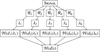 |
Fig. 4 Visualization of the computational graph of the forward model. |
3.4 Inference
In principle, given the prior and likelihood distributions, Eq. (1) allows one to fully determine the posterior distribution by computing the evidence
 (20)
where we have denoted with Ωs the Hilbert space in which s lives. In general, and specifically for the prior and likelihood models described above, the evidence cannot be explicitly evaluated, as it would require integrating over the potentially multi-million- or multi-billion-dimensional space, Ωs. To overcome this problem, we use VI. In VI, the evidence calculation problem is overcome by approximating the posterior distribution directly using a family of tractable distributions 𝒬;α(s|d), parametrized by some variational parameters α. To approximate the posterior, we minimized the Kullback-Leibler divergence,
(20)
where we have denoted with Ωs the Hilbert space in which s lives. In general, and specifically for the prior and likelihood models described above, the evidence cannot be explicitly evaluated, as it would require integrating over the potentially multi-million- or multi-billion-dimensional space, Ωs. To overcome this problem, we use VI. In VI, the evidence calculation problem is overcome by approximating the posterior distribution directly using a family of tractable distributions 𝒬;α(s|d), parametrized by some variational parameters α. To approximate the posterior, we minimized the Kullback-Leibler divergence,
 (21)
with respect to the variational parameters α. In this work, the family of approximating posterior distributions 𝒬;α(s|d) is built using geometric VI (geoVI, Frank et al. (2021)). In geoVI, the posterior is approximated with a Gaussian distribution in a space in which the posterior is approximately Gaussian. This is achieved by utilizing the Fisher information metric, which captures the curvature of the likelihood and the prior distributions. The Fisher metric provides a way to measure the local geometry of the posterior, guiding the creation of a local isometry – a transformation that maps the curved parameter space to a Euclidean space while preserving its geometric properties. In this transformed space, the posterior distribution approximates a Gaussian distribution more closely, allowing the Gaussian variational approximation to be more accurate. Consequently, geoVI can represent non-Gaussian posteriors with high fidelity, improving inference results. By leveraging the geometric properties of the posterior distribution, geoVI offers a powerful extension to traditional VI, enabling more precise and reliable approximations for complex Bayesian models, as the ones presented in this work.
(21)
with respect to the variational parameters α. In this work, the family of approximating posterior distributions 𝒬;α(s|d) is built using geometric VI (geoVI, Frank et al. (2021)). In geoVI, the posterior is approximated with a Gaussian distribution in a space in which the posterior is approximately Gaussian. This is achieved by utilizing the Fisher information metric, which captures the curvature of the likelihood and the prior distributions. The Fisher metric provides a way to measure the local geometry of the posterior, guiding the creation of a local isometry – a transformation that maps the curved parameter space to a Euclidean space while preserving its geometric properties. In this transformed space, the posterior distribution approximates a Gaussian distribution more closely, allowing the Gaussian variational approximation to be more accurate. Consequently, geoVI can represent non-Gaussian posteriors with high fidelity, improving inference results. By leveraging the geometric properties of the posterior distribution, geoVI offers a powerful extension to traditional VI, enabling more precise and reliable approximations for complex Bayesian models, as the ones presented in this work.
4 Results
In Figure 5, we present the reconstruction of the sky flux distribution based on the data shown in Figure 1. Our algorithm’s forward modeling of the X-ray sky enables the decomposition of the signal into point-like, diffuse, and extended-source emission components, providing a more detailed view of the small-scale features of the extended structure of the 30 Doradus C bubble. These reconstructed components are also displayed in Figure 5. From these reconstructions, it is clear that most of the point-like emission is well separated from the diffuse emission, resulting in the first denoised and deconvolved view of this region of the sky as observed by the eROSITA X-ray observatory. Additionally, in Fig. E.2, we show the reconstructed flux for each energy bin, offering a clearer understanding of the color scheme adopted in Fig. 5. All the final reconstructions have been obtained using the geoVI algorithm. For the spatial distribution, we choose a resolution of 1024 × 1024 pixels. For the spectral distribution, we have chosen 3 energy bins corresponding to the energy ranges between 0.2–0.1 keV, 1.0–2.0 keV, and 2.0–4.5 keV, respectively. The variational approximation to the posterior was estimated using eight samples, corresponding to four pairs of antithetic samples. We considered the posterior approximation converged when the posterior expectation values of the signals of interest, such as the reconstructed sky flux field, exhibited no significant changes between consecutive iterations of the VI algorithm. Specifically, we considered the algorithm converged after at least three consecutive geoVI iterations during which the mean squared weighted deviations remained below 1.05. The runtime for the reconstruction was approximately one day on a CPU for a single module, and around two days for all five analyzed telescope modules. By adopting a fully probabilistic approach, we leverage posterior samples to assess how well the model assumptions align with the observed data. In particular, in the presence of shot noise, we defined the posterior mean of the noise weighted residual (NWR) as
 (22)
where λ(s) is the expected number of counts predicted by the model, d is the observed data, and NS is the number of approximate posterior samples. Here, the posterior average over 𝒬;α is approximated by the sample average over the corresponding posterior samples
(22)
where λ(s) is the expected number of counts predicted by the model, d is the observed data, and NS is the number of approximate posterior samples. Here, the posterior average over 𝒬;α is approximated by the sample average over the corresponding posterior samples  . These residuals are particularly useful for identifying model inconsistencies, which may indicate areas for improving the instrument’s description as well as point to potential calibration improvements. We explore this possibility further in the following section (Sect. 5).
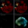 |
Fig. 5 Posterior mean of the SN1987A reconstruction. The top panels display on the left the reconstruction of the sky and on the right the separated diffuse emission. The bottom panels display the reconstruction of the point-like emission (left) and a zoom into the reconstruction of the diffuse emission from 30 Doradus C (right) as marked in Fig. 1. We convolve the point sources with an unnormalized Gaussian kernel with standard deviation σ = 0.5, in order to make them visible on printed paper. The different colors represent the logarithmic intensities in the three energy channels 0.2–0.1 keV, 1.0–2.0 keV, and 2.0–4.5 keV and are depicted in red, green, and blue, respectively. |
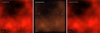 |
Fig. 6 Visualization of the validation of the imaging algorithm. Left: simulated X-ray sky. Center: simulated X-ray data generated as shown in Fig. 4. Right: reconstructed X-ray sky. |
5 Validation and discussion
The discussion is divided into two parts. First, in Sect. 5.1, we validate the general consistency of the presented algorithm using a simulated sky and simulated data, which also motivates the detection threshold for point sources. In the second part, Sect. 5.2, we discuss the results of the reconstruction presented in Sect. 4, along with corresponding diagnostics, such as the NWRs.
5.1 Validation
Generative modeling allows prior models of the sky to be generated, as described in Sect. 3.2. These prior models can be used to validate the consistency of the presented algorithm. In particular, we look at prior samples of the X-ray sky, composed of point sources and diffuse emission, with a FOV of 1024 arcsec. Using the same resolution as for the actual reconstruction, this leads to 256 ×256 pixels. We pass the prior samples through the forward model shown in Fig. 4, including all five TMs, which gives us simulated data. Figure 6 shows the considered prior sample of the X-ray sky as well as the corresponding simulated data passed through the eROSITA response and affected by Pois- sonian noise. The simulated data per TM and the underlying simulated sky per energy bin is shown in the Appendix D in Figs. D.1 and D.2. Using the simulated data  , our aim was to apply the algorithm presented above to estimate the posterior
  through VI posterior samples. We then evaluated how well the corresponding prior ;(s) is reconstructed and determined the corresponding uncertainty in that estimate. The right side of Fig. 6 shows the reconstructed prior sample. Component separation, deconvolution, and denoising techniques show strong performance when applied to simulated data. They effectively recover the underlying signal.
To validate the results shown in Fig. 6, we used a set of validation metrics that we have access to due to the probabilistic approach of the algorithm. These metrics are intended to provide further insight into the residuals between the simulated X-ray sky and its reconstruction, as well as the uncertainty of the algorithm at each pixel.
Accordingly, we show in the appendix the standard deviation of the posterior samples in Fig. D.4, which gives us a measure of the uncertainty of the algorithm. To examine the residuals, we defined the standardized error as the relative residual between the ground truth, Sgt, and the posterior mean, s,
 (23)
to check for differences between the ground truth and the reconstruction. This standardized error is shown for each energy bin in Appendix D in Fig. D.5. The image shows that point sources are not detected or are misplaced in some areas. This highlights the need for a detection threshold for point sources in the reconstruction to ensure the correctness as also indicated in the hyper parameter search in Appendix C. To validate the detection threshold further we use posterior samples,
(23)
to check for differences between the ground truth and the reconstruction. This standardized error is shown for each energy bin in Appendix D in Fig. D.5. The image shows that point sources are not detected or are misplaced in some areas. This highlights the need for a detection threshold for point sources in the reconstruction to ensure the correctness as also indicated in the hyper parameter search in Appendix C. To validate the detection threshold further we use posterior samples,  , of the approximated posterior, Q(s|d), for the point source component in order to get the absolute sample-averaged two-dimensional histogram of the standardized error only for point sources,
  , where,
 (24)
(24)
Figure 7 shows the sample-averaged histogram together with the detection threshold, θ, analytically set for this reconstruction in the Appendix C. The figure shows that, even above the threshold, the standardized error for many point sources remains close to 1. These sources are relevant but not identified in the reconstruction due to noise and instrumental effects. This is also evident in Figure 6, which compares the ground truth to the reconstructed signal. Importantly, this behavior is still acceptable: the purpose of the threshold is not to guarantee detection of all real sources, but rather to control false detections, i.e., the appearance of point sources where none exist. As the diagram indicates, such spurious detections may occur below the threshold. Point sources that are clearly identified are highlighted in the gray box in Figure 7. This interpretation is further supported by Figure D.5 in the appendix. In summary, below the detection threshold, the histogram shows two effects, undetected or misplaced point sources and possible noise overfitting, which are eliminated by cutting the point sources below the detection threshold to ensure the consistency of the reconstruction. We apply the same cuts to the reconstruction shown in Sect. 4. We note that the threshold on the reconstructed point source field is applied only a posteriori to isolate emission from reliably detected point sources. Consequently, unresolved point sources remain statistically distributed between the diffuse emission component and the underlying inverse-Gamma distributed field of faint, unresolved point sources. This statistical separation is further guided by the inferred spatial and spectral correlation kernel of the diffuse emission: since spatial correlations are learned during inference, flux from unresolved point sources is more likely to be correctly assigned to the true diffuse component. However, while this holds true for synthetic observations, additional extinction processes in real observational data render this separation even less constrained.
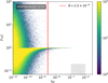 |
Fig. 7 Two-dimensional histogram of the standardized error (Eq. (24)) for the point sources. The histogram is plotted together with the lowest detection threshold, θ = 2.5 × 10⁻⁹, calculated for the region with the longest observation time in Appendix C. The colorbar shows the counts per bin in the two-dimensional histogram, i.e., higher values correspond to more frequent combinations of standardized error and ground truth flux. |
5.2 Discussion of results
The results of the algorithm described above, applied to the eROSITA LMC data, are shown in Sect. 4. Fig. 5 shows the LMC in a deconvolved, denoised and decomposed view. The full image of the LMC is shown, as well as the separated components of the point sources, the diffuse structures of the LMC, and the extended sources of 30 Doradus C. As a result of the inference, we get posterior samples of the approximated posterior probability Q(s|d). Given these posterior samples, we can calculate a measure of uncertainty of the reconstruction, which is in this case given by the standard deviation. The corresponding plots of the standard deviation per energy bin for the reconstruction shown in Fig. 5 is shown in Appendix E in Fig. E.3. As expected, we can see that the uncertainty is higher in regions with a high number of photon counts. This reflects the fact that in regions of higher flux the uncertainty is also higher.
Analyzing the component separation in Fig. 5, it can be seen that there is still a halo around the central SN1987A source, which can have two different causes. First, it could be due to a detection pile-up effect caused by the high fluxes from these sources (Davis 2001). Second, it could be due to a mismodeling of the instruments caused by calibration mismatches. In order to check for possible calibration issues, we performed single- TM reconstructions, which only took the data and the response functions for one of the TMs each into account. The results of the single-TM reconstructions per energy bin are shown in Appendix E in Fig. E.1. These images give us a great insight into possible calibration inconsistencies together with the corresponding NWRs (Eq. (22)) per TM and energy bin, which are shown in Figs. E.4 and E.5. The convolution of the NWRs with the FOV-averaged PSF visually emphasizes correlated errors and thus highlights problems with calibration, see E.6. In particular, the reconstruction for TM2 suggests both pile-up issues and mismatches in the calibration files, such as the PSF and dead pixels. Although we incorporated information about the dead pixels into the inference, the number of dead pixels accounted for seems to be insufficient. The reconstruction clearly indicates that there are likely additional dead pixels in this area.
Figure 8 shows a comparison of the diffuse structures around the Tarantula Nebula in the eROSITA data, zoomed in for both a single TM and all five TMs. We note that it is more difficult to separate point-like from diffuse emission using all the telescope modules. This is likely due to possible calibration inconsistencies in comparison with the single-TM reconstructions. We note that our derived point source component provides a foundation for future catalog creation, although a direct comparison with the existing SRG/eROSITA catalog by Merloni et al. (2024) is beyond the scope of this study. Such a comparison would require extensive calibration and validation, particularly given the calibration artifacts identified in our reconstructions and the fact that our analysis did not utilize the full available dataset across the entire field of view. Nevertheless, our methodology demonstrates the feasibility of automated point source extraction from Bayesian reconstructions, highlighting a promising direction for future systematic studies and catalog validation efforts. Since in this method we define a threshold for the reconstructed point source field, we quantify the flux discarded by the point source thresholding process and assess its relevance in Appendix E.
Figure 9 gives a view of Chandra data for the region of interest of the LMC, binned to 1024 × 1024 spatial and 3 spectral pixels. Specifically, we chose a 4 arcsec resolution to match the chosen eROSITA resolution. In Fig. 9, we plot the data using the same plotting routine and color-coding for Chandra and eROSITA. Compared to eROSITA data and reconstruction, Chandra provides finer detail due to its higher spatial resolution (0.5 arcsec). This enables us to confirm that the small-scale features in this eROSITA reconstruction – resolved through PSF deconvolution and shot noise removal – are real and not artifacts.
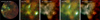 |
Fig. 8 Zoom-in of the reconstruction of diffuse emission from the Tarantula Nebula. From left to right the panels show the zoom area on the plot of the eROSITA LMC data, the zoomed LMC data for TM1, the corresponding single-TM diffuse emission reconstruction for TM1, the zoomed data for all five TMs, and the diffuse emission reconstruction by means of all five observations. |
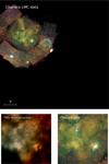 |
Fig. 9 Chandra LMC data. The top panel shows Chandra data, as specified in Table B.1, in the region of the LMC. The bottom panels show the corresponding zoom-ins of our eROSITA reconstruction of the diffuse emission based on the data of TM1 and the Chandra data on the fine-scale structures of the Tarantula Nebula, as shown in Fig. 8. |
6 Conclusion
In conclusion, this paper presents the first Bayesian reconstruction of the eROSITA EDR data, providing a denoised, deconvolved, and separated view of the diffuse and point-like sources in the LMC8. The presented algorithm enables the spatio-spectral reconstruction of the LMC, incorporating its observation by the five different TMs of TM8. Ultimately, the reconstruction shows distinct fine-scale structures in the diffuse emission of the LMC and deconvolved, sharp point sources, which are barely seen from the eROSITA data and verified via the comparison with higher resolved Chandra data. Thus, the presented results have the potential to assist in the further analysis of the diffuse X-ray emission as done by Sasaki et al. (2022) without any noise or point source contributions or effects from the PSF. It also allows the point source catalog to be refined by considering only the point source component. Due to the generative nature of the algorithm we are able to generate simulated data, on which we tested the consistency of the reconstruction. The underlying building blocks of the implementation are publicly available (Eberle et al. 2024) and can therefore be used to image other eROSITA observations as well.
The presented algorithm uses an additional component in the region of 30 Doradus C. Such additional components in certain regions allow to image such extended objects which overlap with the emission from the hot phase of the interstellar medium (ISM) and point sources and have a very different correlation structure. In this way, not only the general diffuse and point source emission can be decomposed, but also the diffuse emission from the hot phase of the ISM and from extended sources such as 30 Doradus C can be distinguished. In this work, the additional component for the extended source was set by hand. For future work, we aim to automate this and to find the extended sources for high excitations in the latent space.
There are also several areas for further investigation. The algorithm presented here can be useful to check the calibration using single TM reconstructions and diagnostics such as the NWRs, which are readily available due to the algorithm’s probabilistic nature. Future work could focus on improving the spectral resolution to allow further insight into the spectra of the different components. In addition, work is underway to extend the applicability to eROSITA field scans and all-sky surveys. Finally, the flexibility of the algorithm extends beyond eROSITA. Its general framework can be adapted to other photon-counting observatories, such as Chandra, XMM-Newton, and more, enabling high-resolution imaging across diverse instruments. By making the instrument models publicly available through J-UBIK, we aim to facilitate future developments and applications, including Bayesian multi-messenger imaging of specific celestial objects.
Acknowledgements
V. Eberle, M. Guardiani, and M. Westerkamp acknowledge financial support from the German Aerospace Center and Federal Ministry of Education and Research through the project Universal Bayesian Imaging Kit – Information Field Theory for Space Instrumentation (Förderkennzeichen 50OO2103). P. Frank acknowledges funding through the German Federal Ministry of Education and Research for the project ErUM-IFT: Informationsfeldtheorie für Experimente an Großforschungsanlagen (Förderkennzeichen: 05D23EO1). This work is based on data from eROSITA, the soft X-ray instrument aboard SRG, a joint Russian-German science mission supported by the Russian Space Agency (Roskosmos), in the interests of the Russian Academy of Sciences represented by its Space Research Institute (IKI), and the Deutsches Zentrum für Luft- und Raumfahrt (DLR). The SRG spacecraft was built by Lavochkin Association (NPOL) and its subcontractors, and is operated by NPOL with support from the Max Planck Institute for Extraterrestrial Physics (MPE). The development and construction of the eROSITA X-ray instrument was led by MPE, with contributions from the Dr. Karl Remeis Observatory Bamberg & ECAP (FAU Erlangen-Nuernberg), the University of Hamburg Observatory, the Leibniz Institute for Astrophysics Potsdam (AIP), and the Institute for Astronomy and Astrophysics of the University of Tübingen, with the support of DLR and the Max Planck Society. The Argelander Institute for Astronomy of the University of Bonn and the Ludwig Maximilians Universität Munich also participated in the science preparation for eROSITA. The eROSITA data shown here were processed using the eSASS software system developed by the German eROSITA consortium.
References
- Arras, P., Baltac, M., Enßlin, T. A., et al. 2019, Astrophysics Source Code Library [Google Scholar]
- Arras, P., Frank, P., Haim, P., et al. 2022, Nat. Astron., 6, 259 [NASA ADS] [CrossRef] [Google Scholar]
- Brunner, H., Boller, T., Coutinho, D., et al. 2018, SPIE Conf. Ser., 10699, 106995G [Google Scholar]
- Brunner, H., Liu, T., Lamer, G., et al. 2022, A&A, 661, A1 [NASA ADS] [CrossRef] [EDP Sciences] [Google Scholar]
- Burrows, D. N., Michael, E., Hwang, U., et al. 2000, ApJ, 543, L149 [Google Scholar]
- Calderwood, T., Dobrzycki, A., Jessop, H., & Harris, D. E. 2001, in Astronomical Society of the Pacific Conference Series, 238, Astronomical Data Analysis Software and Systems X, eds. J. Harnden, F. R., F. A. Primini, & H. E. Payne, 443 [Google Scholar]
- Cooley, J. W., & Tukey, J. W. 1965, Math. Computat., 19, 297 [Google Scholar]
- Davis, J. E. 2001, ApJ, 548, 1010 [Google Scholar]
- Ebeling, H., & Wiedenmann, G. 1993, Phys. Rev. E, 47, 704 [CrossRef] [Google Scholar]
- Eberle, V., Guardiani, M., Westerkamp, M., et al. 2024, J-UBIK: The JAX- accelerated Universal Bayesian Imaging Kit [Google Scholar]
- Edenhofer, G., Frank, P., Roth, J., et al. 2024, JOSS, 9, 6593 [Google Scholar]
- Enßlin, T. A. 2019, Ann. Phys., 531, 1800127 [Google Scholar]
- Enßlin, T. A., Frommert, M., & Kitaura, F. S. 2009, Phys. Rev. D, 80, 105005 [Google Scholar]
- Frank, P., Leike, R., & Enßlin, T. A. 2021, Entropy, 23, 853 [NASA ADS] [CrossRef] [Google Scholar]
- Freeman, P. E., Kashyap, V., Rosner, R., & Lamb, D. Q. 2002, ApJSuppl. Ser., 138, 185 [Google Scholar]
- Garmire, G. P., Bautz, M. W., Ford, P. G., Nousek, J. A., & Ricker, G. R. J. 2003, SPIE Conf. Ser., 4851, 28 [NASA ADS] [Google Scholar]
- Guglielmetti, F., Fischer, R., & Dose, V. 2009, MNRAS, 396, 165 [NASA ADS] [CrossRef] [Google Scholar]
- Haberl, F., Geppert, U., Aschenbach, B., & Hasinger, G. 2006, A&A, 460, 811 [NASA ADS] [CrossRef] [EDP Sciences] [Google Scholar]
- Kingma, D. P., Salimans, T., & Welling, M. 2015, Variational Dropout and the Local Reparameterization Trick [Google Scholar]
- Knollmüller, J., & Enßlin, T. A. 2020, Metric Gaussian Variational Inference [Google Scholar]
- Liu, T., Merloni, A., Comparat, J., et al. 2022, A&A, 661, A27 [NASA ADS] [CrossRef] [EDP Sciences] [Google Scholar]
- Matsuura, M., Boyer, M., Arendt, R. G., et al. 2024, MNRAS, 532, 3625 [Google Scholar]
- Merloni, A., Lamer, G., Liu, T., et al. 2024, A&A, 682, A34 [NASA ADS] [CrossRef] [EDP Sciences] [Google Scholar]
- Nagy, J. G., & O’Leary, D. P. 1997, in Advanced Signal Processing: Algorithms, Architectures, and Implementations VII, 3162, SPIE, 388 [Google Scholar]
- Predehl, P., Andritschke, R., Arefiev, V., et al. 2021, A&A, 647, A1 [EDP Sciences] [Google Scholar]
- Pumpe, D., Reinecke, M., & Enßlin, T. A. 2018, A&A, 619, A119 [NASA ADS] [CrossRef] [EDP Sciences] [Google Scholar]
- Sanders, J. S., Fabian, A. C., Russell, H. R., Walker, S. A., & Blundell, K. M. 2016, Mon. Not. R. Astron. Soc., 460, 1898 [Google Scholar]
- Sasaki, M., Knies, J., Haberl, F., et al. 2022, A&A, 661, A37 [NASA ADS] [CrossRef] [EDP Sciences] [Google Scholar]
- Schartel, N., & Dahlem, M. 2000, Phys. Blätter, 56, 37 [Google Scholar]
- Scheel-Platz, L. I., Knollmüller, J., Arras, P., et al. 2023, A&A, 680, A2 [NASA ADS] [CrossRef] [EDP Sciences] [Google Scholar]
- Selig, M., & Enßlin, T. A. 2015, A&A, 574, A74 [NASA ADS] [CrossRef] [EDP Sciences] [Google Scholar]
- Selig, M., Bell, M. R., Junklewitz, H., et al. 2013, A&A, 554, A26 [NASA ADS] [CrossRef] [EDP Sciences] [Google Scholar]
- Seppi, R., Comparat, J., Bulbul, E., et al. 2022, A&A, 665, A78 [NASA ADS] [CrossRef] [EDP Sciences] [Google Scholar]
- Seward, F. D., & Charles, P. A. 2010, Exploring the X-ray Universe, 2nd edn. (Cambridge University Press) [Google Scholar]
- Sunyaev, R., Arefiev, V., Babyshkin, V., et al. 2021, A&A, 656, A132 [NASA ADS] [CrossRef] [EDP Sciences] [Google Scholar]
- Truemper, J. 1982, Adv. Space Res., 2, 241 [Google Scholar]
- Westerkamp, M., Eberle, V., Guardiani, M., et al. 2024, A&A, 684, A155 [NASA ADS] [CrossRef] [EDP Sciences] [Google Scholar]
- Zanardo, G., Staveley-Smith, L., Ng, C.-Y., et al. 2013, ApJ, 767, 98 [NASA ADS] [CrossRef] [Google Scholar]
- Zangrandi, F., Jurk, K., Sasaki, M., et al. 2024, A&A, 692, A237 [NASA ADS] [CrossRef] [EDP Sciences] [Google Scholar]
The data used are publicly available at https://erosita.mpe.mpg.de/edr/eROSITAObservations/
The first light EDR image of LMC SN1987A by Haberl et al. is shown in https://www.dlr.de/de/aktuelles/nachrichten/2019/04/20191022_first-light-erosita
To convert the reported fluxes to units of [keV/(arcsec2 ×s)], multiply by 〈ℇ〉i, the average photon energy in keV for each sky reconstruction bin i. The resulting value corresponds then to the mean integrated flux in this energy bin.
Information about the CALDB: https://erosita.mpe.mpg.de/edr/DataAnalysis/esasscaldb.html
Details in Appendix A.
More information about the eSASS software developed by the eROSITA Team can be found here: https://erosita.mpe.mpg.de/edr/DataAnalysis/
Details in Appendix A.
The reconstructed fields can be found at https://doi.org/10.5281/zenodo.16918521
Further information on the eSASS pipeline can also be found at https://erosita.mpe.mpg.de/edr/dataanalysis/.
A further description of the flags can be found at https://erosita.mpe.mpg.de/edr/dataanalysis/evtool_doc.html.
Appendix A eROSITA observation of LMC SN1987A
The CalPV data centered on SN1987A in the LMC were preprocessed using the eSASS pipeline, which is described in detail by Brunner et al. (2018) and Predehl et al. (2021)9. In particular, the data was extracted and manipulated using the eSASS evtool command. We list the flag values we chose for the evtool command10 in Table A.1. We computed the exposure maps for the eROSITA event files using the eSASS expmap command and the corresponding flags in A.2. The data per energy bin and per TM is shown in Fig. A.1. The corresponding exp- soure maps summed over the 5 TMs are shown in Fig. A.2 The PSFs used for the PSF linear patched convolution representation can be found in tm[1-7]_2dpsf_190219v05.fits in the CALDB. The effective area for the individual CA can be found in tm[1-7]_arf_filter_000101v02.fits in the CALDB.
Flags and their corresponding data types for evtool where tmid, where tmid ∈ {1, 2, 3, 4,6} and (emin, emax) ∈ {(0.2, 1.0), (1.0, 2.0), (2.0, 4.5)}
Flags and their corresponding data types for expmap, where tmid ∈ {1, 2, 3, 4, 6} and (emin, emax) ∈ {(0.2, 1.0), (1.0, 2.0), (2.0, 4.5)}
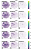 |
Fig. A.1 Visualization of eROSITA data per energy bin in number of counts from left to right, 0.2 - 0.1 keV, 1.0 - 2.0 keV, and 2.0 - 4.5 keV for TM1 to TM6 from top to bottom. |
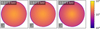 |
Fig. A.2 eROSITA exposure maps summed over all 5 TMs. |
Appendix B Chandra observations of the LMC
In Fig. 9 the Chandra data of certain regions of the LMC is shown. The according observations, which were taken into account, are specified in this section in table B.1.
Appendix C Hyperparameter search
The prior model described in Sect. 3.2 requires choosing a set of hyperparameters, which describe the mean and standard deviation of the Gaussian processes modeling the prior. The meaning of the specific hyperparameters of the correlated field is more precisely described in Arras et al. (2022). In particular, the offset mean of the correlated field parametrizes the mean of τ in Eq 3 and therefore the mean of the log-normal flux. Accordingly, we take the exposure-corrected data, de, shown in Fig. 1 and calculate its mean 〈de〉 and set both the offset mean of φln and φln,b to log 〈de〉 = −19.9.
We use the information on the detection threshold to set the hyperparameters for the inverse gamma distribution used for the point sources. In particular we set the mean m of the inverse gamma distribution as the sum of all fluxes from point sources which are higher than the detection threshold θ divided by the total number of pixels.
To determine the detection threshold θ, we set a minimum signal to noise ratio (S/N), γmin, that is required to reliably detect a source. Essentially, for a source to be detected, the S/N γ in each pixel must be higher than this set threshold, γmin. Specifically, for Poisson data, the S/N is given by  , where λ is the expected number of counts in a pixel. We set γmin based on the confidence level we want for detection. In this case, we aim for a 99% confidence level, meaning there is a 99% probability that any observed signal is not just a random fluctuation,
 (C.1)
which leads to λmin = 4.6 and, consequently,
(C.1)
which leads to λmin = 4.6 and, consequently,  . The pixel-wise detection threshold θi is then defined, via the smallest flux, which can be reliably detected in each pixel i, which is given via λmin and the exposure in the corresponding pixel, Ei
 (C.2)
(C.2)
These θi’s are used as a pixel wise criterion for the acceptance of a point source in the final plots. This line of thought can also be used in order to set priors for the inverse gamma component. Therefore, we want to find an overall detection threshold for the whole image, which is then defined via maximal exposure, Emax
 (C.3)
(C.3)
Eventually, this leads to a mean m = 2.08 × 10⁻⁹ of the inverse gamma distribution. The mode M of the inverse gamma distribution should be even further below the detection threshold. In particular, we thus assume that the S/N ratio for the mode is much lower, i.e. γmin = 0.1,
 (C.4)
(C.4)
Having the mean and the mode, we can use these in order to calculate the hyper-parameters α and q of the inverse gamma distribution via
 (C.5)
(C.5)
 (C.6)
(C.6)
A prior sample drawn from the prior given these hyperparameters can be seen in Fig. 2.
Appendix D Validation diagnostics
This section provides supplementary plots that offer further insights into the validation analysis discussed in Sect. 5.1. These plots show in particular the images of the simulated sky, the simulated data, and the corresponding reconstruction. These are shown as an RGB image in Fig. 6 as plots per energy, which serve to enhance the understanding of the color bar for the RGB image. In particular the data per energy bin and TM is presented in Fig. D.1, the underlying simulated sky per energy bin is shown in Fig. D.2 and the reconstructed sky per energy bin is illustrated in Fig. D.3. Furthermore, we display the uncertainty in the reconstruction by means of the standard deviation for each energy bin in Fig. D.4. Fig. D.5 shows the standardized error for each energy bin.
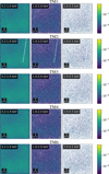 |
Fig. D.1 Visualization of the exposure corrected simulated data per energy bin from left to right, 0.2-1.0 keV, 1.0-2.0 keV, and 2.0-4.5 keV for TM1 to TM6 from top to bottom. |
Appendix E Results diagnostics
Here, we show additional plots corresponding to the reconstruction of SN1987A in the LMC as seen by SRG/eROSITA in the CalPV phase. First, we display the reconstruction shown in Fig. 5 per energy bin in Fig. E.2 to give a better understanding of the color bar used. We also show the corresponding uncertainty in the form of the standard deviation per energy bin in Fig. E.3. Finally, we also performed single TM reconstructions, the results of which are shown per TM in Fig. E.1. Important diagnostic measures to check for possible calibration inconsistencies in the single TM reconstructions are the NWRs (Eq. (22)), which are shown per TM and energy bin in Fig. E.4 and Fig. E.5. Additionally, in Fig. E.6 we display the convolved noise-weighted residuals (CNWRs), defined as
 (E.1)
where Ô denotes a Gaussian kernel with a standard deviation corresponding to the full width at half maximum (FWHM) of the average eROSITA PSF (26 arcsec, see Predehl et al. 2021). This convolution suppresses pixel-scale fluctuations and highlights mismatches on physically meaningful angular scales. As expected, the CNWR maps show minor residuals at the positions of a few bright point sources, already discussed in the text and attributed to calibration uncertainties. Finally, in Fig. E.7, we provide a quantitative assessment of the flux discarded when applying the point source detection threshold defined in Eq. (C.3), focusing on TM1. The left panel shows the expected count rate λt associated with point source emission below the detection threshold. We find that λt remains below unity across the field, indicating that no substantial flux is removed. This is further supported by the right panel, which shows the ratio of λt to the expected noise level,
(E.1)
where Ô denotes a Gaussian kernel with a standard deviation corresponding to the full width at half maximum (FWHM) of the average eROSITA PSF (26 arcsec, see Predehl et al. 2021). This convolution suppresses pixel-scale fluctuations and highlights mismatches on physically meaningful angular scales. As expected, the CNWR maps show minor residuals at the positions of a few bright point sources, already discussed in the text and attributed to calibration uncertainties. Finally, in Fig. E.7, we provide a quantitative assessment of the flux discarded when applying the point source detection threshold defined in Eq. (C.3), focusing on TM1. The left panel shows the expected count rate λt associated with point source emission below the detection threshold. We find that λt remains below unity across the field, indicating that no substantial flux is removed. This is further supported by the right panel, which shows the ratio of λt to the expected noise level,  , at each pixel. The thresholded flux never exceeds half the local noise level, confirming that the discarded flux is negligible and does not impact the overall reconstruction quality.
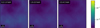 |
Fig. D.2 Visualization of the simulated sky per energy bin (left: 0.2-1.0 keV, center: 1.0-2.0 keV, right: 2.0-4.5 keV) in [1/(arcsec2 × s)]. |
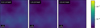 |
Fig. D.3 Visualization of the reconstruction per energy bin (left: 0.2-1.0 keV, center: 1.0-2.0 keV, right: 2.0-4.5 keV) in [1/(arcsec2 × s)]. |
 |
Fig. D.4 Visualization of the standard deviation of the validation reconstruction per energy bin (left: 0.2-1.0 keV, center: 1.0-2.0 keV, right: 2.0-4.5 keV) in [1/(arcsec2 × s)]. |
 |
Fig. D.5 Visualization of the standardized error of the validation reconstruction per energy bin (left: 0.2-1.0 keV, center: 1.0-2.0 keV, right: 2.0-4.5 keV). |
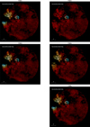 |
Fig. E.1 Results for single-TM reconstructions for TM1, TM2, TM3, TM4, TM6. The different colors represent the logarithmic intensities in the three energy channels 0.2 - 0.1 keV, 1.0 - 2.0 keV, and 2.0 - 4.5 keV and are depicted in red, green, and blue, respectively. |
 |
Fig. E.2 Posterior mean of the sky reconstruction in the different energy bins in [1/(arcsec2 × s)]. |
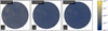 |
Fig. E.3 Standard deviation per energy bin for the reconstruction shown in Figs. 5+E.2 in [1/(arcsec2 × s)]. |
 |
Fig. E.5 Posterior mean of the NWRs for single-TM reconstructions. A value of 1 indicates that the observed data counts lie within one Poisson standard deviation of the reconstructed expected flux λ. |
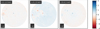 |
Fig. E.6 Posterior mean of the convolved noise-weighted residuals (CNWRs), see Eq. (E.1), obtained by smoothing the pixel-wise NWR with a Gaussian kernel matched to the average eROSITA PSF (FWHM ≃ 26″). The convolution suppresses pixel-scale variations and emphasizes coherent structures. |
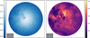 |
Fig. E.7 Thresholded expected point source count rate analysis for TM1. Left panel: Expected count-rate (λt) from point source emission below the detection threshold (Eq. (C.3)), illustrating that it is everywhere below unity, indicating negligible discarded flux. Right panel: Ratio between the thresholded expected point source count rate (λt) and the expected noise ( |

All Tables
Flags and their corresponding data types for evtool where tmid, where tmid ∈ {1, 2, 3, 4,6} and (emin, emax) ∈ {(0.2, 1.0), (1.0, 2.0), (2.0, 4.5)}
Flags and their corresponding data types for expmap, where tmid ∈ {1, 2, 3, 4, 6} and (emin, emax) ∈ {(0.2, 1.0), (1.0, 2.0), (2.0, 4.5)}
All Figures
|
Fig. 1 Visualization of the exposure-corrected eROSITA EDR TM8 data of ObsID 700161 for three energy bins. Red: 0.2–1.0 keV, green: 1.0–2.0 keV, blue: 2.0–4.5 keV. The white box marks the region of 30 Doradus C further discussed in Sect. 3.2. The bright central point-like source underneath the bottom-right corner of the 30 Doradus C box is SN1987A. |
| In the text | |
|
Fig. 2 Visualization of one prior sample drawn from the prior model described in Sect. 3.2 for three energy bins in [1/(arcsec2 × s)]. |
| In the text | |
|
Fig. 3 Visualization of eROSITA PSF approximated by the linear patch convolution algorithm for three energy bins. The different colors represent the logarithmic intensities in the three energy bands. Red: 0.2–1.0 keV, green: 1.0–2.0 keV, blue: 2.0–4.5 keV. |
| In the text | |
|
Fig. 4 Visualization of the computational graph of the forward model. |
| In the text | |
|
Fig. 5 Posterior mean of the SN1987A reconstruction. The top panels display on the left the reconstruction of the sky and on the right the separated diffuse emission. The bottom panels display the reconstruction of the point-like emission (left) and a zoom into the reconstruction of the diffuse emission from 30 Doradus C (right) as marked in Fig. 1. We convolve the point sources with an unnormalized Gaussian kernel with standard deviation σ = 0.5, in order to make them visible on printed paper. The different colors represent the logarithmic intensities in the three energy channels 0.2–0.1 keV, 1.0–2.0 keV, and 2.0–4.5 keV and are depicted in red, green, and blue, respectively. |
| In the text | |
|
Fig. 6 Visualization of the validation of the imaging algorithm. Left: simulated X-ray sky. Center: simulated X-ray data generated as shown in Fig. 4. Right: reconstructed X-ray sky. |
| In the text | |
|
Fig. 7 Two-dimensional histogram of the standardized error (Eq. (24)) for the point sources. The histogram is plotted together with the lowest detection threshold, θ = 2.5 × 10⁻⁹, calculated for the region with the longest observation time in Appendix C. The colorbar shows the counts per bin in the two-dimensional histogram, i.e., higher values correspond to more frequent combinations of standardized error and ground truth flux. |
| In the text | |
|
Fig. 8 Zoom-in of the reconstruction of diffuse emission from the Tarantula Nebula. From left to right the panels show the zoom area on the plot of the eROSITA LMC data, the zoomed LMC data for TM1, the corresponding single-TM diffuse emission reconstruction for TM1, the zoomed data for all five TMs, and the diffuse emission reconstruction by means of all five observations. |
| In the text | |
|
Fig. 9 Chandra LMC data. The top panel shows Chandra data, as specified in Table B.1, in the region of the LMC. The bottom panels show the corresponding zoom-ins of our eROSITA reconstruction of the diffuse emission based on the data of TM1 and the Chandra data on the fine-scale structures of the Tarantula Nebula, as shown in Fig. 8. |
| In the text | |
|
Fig. A.1 Visualization of eROSITA data per energy bin in number of counts from left to right, 0.2 - 0.1 keV, 1.0 - 2.0 keV, and 2.0 - 4.5 keV for TM1 to TM6 from top to bottom. |
| In the text | |
|
Fig. A.2 eROSITA exposure maps summed over all 5 TMs. |
| In the text | |
|
Fig. D.1 Visualization of the exposure corrected simulated data per energy bin from left to right, 0.2-1.0 keV, 1.0-2.0 keV, and 2.0-4.5 keV for TM1 to TM6 from top to bottom. |
| In the text | |
|
Fig. D.2 Visualization of the simulated sky per energy bin (left: 0.2-1.0 keV, center: 1.0-2.0 keV, right: 2.0-4.5 keV) in [1/(arcsec2 × s)]. |
| In the text | |
|
Fig. D.3 Visualization of the reconstruction per energy bin (left: 0.2-1.0 keV, center: 1.0-2.0 keV, right: 2.0-4.5 keV) in [1/(arcsec2 × s)]. |
| In the text | |
|
Fig. D.4 Visualization of the standard deviation of the validation reconstruction per energy bin (left: 0.2-1.0 keV, center: 1.0-2.0 keV, right: 2.0-4.5 keV) in [1/(arcsec2 × s)]. |
| In the text | |
|
Fig. D.5 Visualization of the standardized error of the validation reconstruction per energy bin (left: 0.2-1.0 keV, center: 1.0-2.0 keV, right: 2.0-4.5 keV). |
| In the text | |
|
Fig. E.1 Results for single-TM reconstructions for TM1, TM2, TM3, TM4, TM6. The different colors represent the logarithmic intensities in the three energy channels 0.2 - 0.1 keV, 1.0 - 2.0 keV, and 2.0 - 4.5 keV and are depicted in red, green, and blue, respectively. |
| In the text | |
|
Fig. E.2 Posterior mean of the sky reconstruction in the different energy bins in [1/(arcsec2 × s)]. |
| In the text | |
|
Fig. E.3 Standard deviation per energy bin for the reconstruction shown in Figs. 5+E.2 in [1/(arcsec2 × s)]. |
| In the text | |
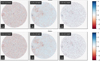 |
Fig. E.4 Continued in Fig. E.5. |
| In the text | |
|
Fig. E.5 Posterior mean of the NWRs for single-TM reconstructions. A value of 1 indicates that the observed data counts lie within one Poisson standard deviation of the reconstructed expected flux λ. |
| In the text | |
|
Fig. E.6 Posterior mean of the convolved noise-weighted residuals (CNWRs), see Eq. (E.1), obtained by smoothing the pixel-wise NWR with a Gaussian kernel matched to the average eROSITA PSF (FWHM ≃ 26″). The convolution suppresses pixel-scale variations and emphasizes coherent structures. |
| In the text | |
|
Fig. E.7 Thresholded expected point source count rate analysis for TM1. Left panel: Expected count-rate (λt) from point source emission below the detection threshold (Eq. (C.3)), illustrating that it is everywhere below unity, indicating negligible discarded flux. Right panel: Ratio between the thresholded expected point source count rate (λt) and the expected noise ( |
| In the text | |
Current usage metrics show cumulative count of Article Views (full-text article views including HTML views, PDF and ePub downloads, according to the available data) and Abstracts Views on Vision4Press platform.
Data correspond to usage on the plateform after 2015. The current usage metrics is available 48-96 hours after online publication and is updated daily on week days.
Initial download of the metrics may take a while.