© The Authors 2026

1. Introduction

Pulsar timing array (PTA) collaborations provide compelling evidence for the existence of a stochastic gravitational wave (GW) background by measuring both a common-spectrum stochastic process (Agazie et al. 2023c; Antoniadis et al. 2023a,b; Reardon et al. 2023a; Zic et al. 2023; Reardon et al. 2023b; Xu et al. 2023) and finding strong evidence for Hellings-Downs angular correlations (Hellings & Downs 1983). The most conservative explanation for the origin of the background is supermassive black hole (SMBH) binaries (Antoniadis et al. 2024; Agazie et al. 2023d; Ellis et al. 2024b; Bi et al. 2023; Ellis et al. 2024c; Raidal et al. 2024), although cosmological sources, such as cosmic superstrings, phase transitions, and domain walls, can also explain the data equally well (Antoniadis et al. 2024; Afzal et al. 2023; Figueroa et al. 2024; Ellis et al. 2024a). Unlike a GW background originating from SMBHs, cosmological sources, after accounting for intrinsic kinematic anisotropy (Cruz et al. 2024a), generate an isotropic background, making the detection of anisotropy within the GW background measurements a powerful indicator that SMBH binaries are the source.

Methods for measuring GW background anisotropies using PTAs have been well explored (Mingarelli et al. 2013; Cornish & van Haasteren 2014; Allen et al. 2024; Hotinli et al. 2019), and investigations into simulated circular SMBH binary populations have examined both the magnitude and frequency scaling of anisotropies in these models (Taylor & Gair 2013; Taylor et al. 2020; Gardiner et al. 2024; Sato-Polito & Kamionkowski 2024; Sah et al. 2024). With the most recent constraint on measured anisotropy placed at C_l > 0/C_l = 0 < 0.2 for the Bayesian 95% upper limit by NANOGrav (Agazie et al. 2023e), we can already derive information about SMBH binary populations based on the amount of anisotropy they produce in the GW signal. Current and future experiments will, within relatively short time frames Pol et al. (2022), Lemke et al. (2025), Depta et al. (2025), significantly improve the sensitivity to anisotropies, enabling further model discrimination. Different models of SMBH binary populations can also be distinguished by measuring the circular polarisation of gravitational waves (Cruz et al. 2024b).

The distribution of fluctuations in the GW spectrum is dominated by a relatively small number of loud SMBH binaries (Ellis et al. 2023, 2024b; Sato-Polito & Zaldarriaga 2025; Xue et al. 2025). Similarly, the loudest binaries generate significant anisotropy in the background. This article outlines the statistical properties of GW background anisotropies by deriving the distributions of the angular power spectrum coefficients. Although the mean of the coefficients C_l > 0/C_l = 0 is independent of l, their distributions differ. The distributions are highly non-Gaussian and can be quite wide. Thus, to make reliable inferences about SMBH populations based on GW anisotropy measurements, one cannot rely solely on the mean of C_l > 0/C_l = 0.

Processes that govern the orbital decay of SMBH binaries and lead to their eventual merger are poorly understood. To reproduce the spectral shape of the GW background, either environmental effects or high eccentricities are favoured (Antoniadis et al. 2024; Agazie et al. 2023d; Ellis et al. 2024b; Bi et al. 2023; Raidal et al. 2024; Chen et al. 2024). This does not imply that circular SMBH binaries are excluded by the data (Antoniadis et al. 2023b; Agazie et al. 2023b). These considerations can also be affected by potential systematic biases that arise during recovery of the GW signal from the data Valtolina et al. (2024).

Although the timescale for the evolution of a single binary is similar in both environmental and eccentric models, the physical process is very different. Binary evolution can be driven by its interactions with the surrounding matter before the GW emission dominates at very small separations. This process reduces the amplitude of the GW background at lower frequencies, which are emitted by wider binaries (Chen et al. 2017b,a; Taylor et al. 2017; Bonetti et al. 2018; Chen et al. 2020; Alonso-Álvarez et al. 2024). Highly eccentric binaries evolve faster at low orbital frequencies by emitting GWs at multiple harmonics, thereby contributing to the GW background at higher frequencies (Enoki & Nagashima 2007; Sesana 2013; Chen et al. 2017b; Fastidio et al. 2024). This results in a spectrum similar to that obtained with environmental energy loss. However, the GW background from eccentric binaries is significantly more isotropic because a larger number of binaries contribute within a given frequency range. Therefore, GW background anisotropy is an observable that can discriminate not only between cosmological and astrophysical sources but also between the models of SMBH binary evolution.

This paper is organised as follows. In Section 2, we review the SMBH models considered and the computation of the GW background for a given SMBH scenario. The GW background anisotropy and its statistical properties are derived in Section 3. Section 4 summarises the main results, and their implications are discussed in Section 5. We conclude in Section 6. Some technical results are presented in the appendices.

2. Modelling the SMBH population

Although SMBHs have been found at the centres of many galaxies, their formation mechanisms and evolution remain unclear. If the PTA signal is interpreted as originating from SMBH binaries, varying merger rates and evolutionary scenarios can be compared to observations. In this work, we study four models that describe the GW emission of SMBH binaries. The first two models consider circular binaries: one evolving purely through GW emission and the other through a combination of GW emission and environmental interactions (Ellis et al. 2024b). The remaining two models consider eccentric binaries, again evolving purely through GW emission or through both GW emission and environmental interactions (Raidal et al. 2024). Their GW-related characteristics are summarised in Fig. 1.

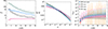Fig. 1. Gravitational wave (GW) characteristics of the SMBH binary population for four different SMBH models: purely GW driven inspirals (GW only), inspirals with environmental effects (GW+env), inspirals of eccentric SMBH binaries (GW+ecc), and inspirals of eccentric SMBH binaries with environmental effects (GW+ecc+env). Left panel: Median (solid line) and mean (dashed line) number of the strongest sources contributing half the signal at each PTA frequency band. Middle panel: Distributions of contributions from individual binaries at 1.98 nHz (solid lines) and 27.68 nHz (dashed lines). Right panel: Distributions of the GW spectra in the n × 1.98 nHz frequency bins compared to NANOGrav 15-year data (yellow violin plots).

The GW background of SMBHs is determined by their merger rate. The differential merger rate of black holes (BHs) in the observer reference frame is¹

$$\begin{array}{c}\hfill \mathrm{d}\lambda =\mathrm{d}\mathcal{M}\mathrm{d}\eta \mathrm{d}z\frac{1}{1+z}\frac{\mathrm{d}{V}_c}{\mathrm{d}z}\frac{\mathrm{d}{R}_{\mathrm{BH}}}{\mathrm{d}\mathcal{M}\mathrm{d}\eta },\end{array}$$(1)

where ℳ, η, and z are the chirp mass, the symmetric mass ratio, and the redshift of the binary. We denote the comoving volume by V_c and the comoving BH merger rate density by R_BH. The BH merger rate was estimated from the halo merger rate R_h given by the extended Press-Schechter formalism (Press & Schechter 1974; Bond et al. 1991; Lacey & Cole 1993):

$$\begin{array}{c}\hfill \begin{array}{cc}\hfill \frac{\mathrm{d}{R}_{\mathrm{BH}}}{\mathrm{d}{m}_1\mathrm{d}{m}_2}=p_{\mathrm{BH}}{\displaystyle \int }& \mathrm{d}{M}_{\mathrm{v},1}\mathrm{d}{M}_{\mathrm{v},2}\frac{\mathrm{d}{R}_h}{\mathrm{d}{M}_{\mathrm{v},1}\mathrm{d}{M}_{\mathrm{v},2}}\hfill \\ \hfill & \times {\displaystyle \prod _{j=1,2}}\frac{\mathrm{d}P(m_j|M_{\ast }(M_{\mathrm{v},j},z))}{\mathrm{d}{m}_j}.\hfill \end{array}\end{array}$$(2)

Here, m_j are the masses of the merging BHs, M_v, j are the virial masses of their host halos, and p_BH ≤ 1, treated as a free parameter, combines the SMBH occupation fraction in galaxies with the BH merger efficiency following host halo mergers. The BH masses were obtained using the observed halo mass-stellar mass relation, M_*(M_v, j, z), taken from Girelli et al. (2020) and the global fit stellar mass-BH mass relation Ellis et al. (2024c),

$$\begin{array}{c}\hfill \frac{\mathrm{d}P(m|M_{\ast })}{\mathrm{d}{log}_{10}m}=\mathcal{N}({log}_{10}\frac{m}{M_{\odot }}|a+b{log}_{10}\frac{M_{\ast }}{{10}^{11}{M}_{\odot }},\sigma ),\end{array}$$(3)

with a = 8.6, b = 0.8, and σ = 0.8. Here, $\mathcal{N}(x|\overline{x},\sigma )$ denotes the probability density of a Gaussian distribution with mean $\overline{x}$ and variance σ².

The mean of the GW background spectrum at a given frequency from a population of potentially eccentric SMBH binaries, in its most general form, is given by (Raidal et al. 2024; Ellis et al. 2024b)

$$\begin{array}{c}\hfill \begin{array}{cc}\hfill ⟨\mathrm{\Omega }(f)⟩=\frac{1}{{\rho }_c}{\displaystyle \int \mathrm{d}}\lambda & \mathrm{d}e\mathrm{d}{f}_{\mathrm{b}}\sum _{n=1}^{\infty }\delta (f_{\mathrm{b}}-\frac{f_{\mathrm{r}}}{n})\hfill \\ \hfill & \times P(e|f_{\mathrm{b}})\frac{1+z}{4\pi D_L^2}\frac{\mathrm{d}{E}_n}{\mathrm{d}ln{f}_{\mathrm{b}}},\hfill \end{array}\end{array}$$(4)

where ρ_c is the critical energy density, D_L is the source luminosity distance, P(e|f_b) is the binary eccentricity distribution at a given orbital frequency f_b. The delta function selects binaries whose n-th harmonic contributes to the observed frequency f = f_r/(1 + z). We modelled P(e|f_b) by a power law (see Raidal et al. (2024)) for the eccentric model and P(e|f_b) = δ(e) for the models with circular binaries. Expressing Eq. (4) in terms of binary parameters becomes

$$\begin{array}{c}\hfill \begin{array}{cc}\hfill ⟨\mathrm{\Omega }(f)⟩& ={\displaystyle \int \mathrm{d}}\lambda \mathrm{d}e{\displaystyle \sum _{n=1}^{\infty }}P(e|f_{\mathrm{b}})g_n(e){\mathrm{\Omega }}_c^{(1)}\frac{\mathrm{d}t}{\mathrm{d}ln{f}_{\mathrm{b}}}{|}_{f_{\mathrm{b}}=\frac{f_r}{n}},\hfill \end{array}\end{array}$$(5)

where g_n(e) is the GW power emitted into the n-th harmonic (Peters & Mathews 1963), dt/dlnf_b is the residence time, which is affected by the environment and the eccentricity of the binary (see Appendix A for details), and

$$\begin{array}{c}\hfill {\mathrm{\Omega }}_c^{(1)}\equiv \frac{1}{4\pi D_L^2{\rho }_c}\frac{\mathrm{d}{E}_c}{\mathrm{d}{t}_r}\end{array}$$(6)

represents the GW luminosity of a single circular binary.

It is well known that the mean (5) does not accurately capture the likely realisations of the GW spectrum, because the distributions of the spectral fluctuations are non-Gaussian and have heavy tails favouring large upward fluctuations (Ellis et al. 2023, 2024b; Sato-Polito & Zaldarriaga 2025; Xue et al. 2025). Therefore, it is important to consider statistical fluctuations in the signal at a given measured frequency. These statistical properties can be inferred from the distribution of contributions Ω from individual binaries at a given frequency f:

$$\begin{array}{c}\hfill \begin{array}{cc}\hfill P^{(1)}(\mathrm{\Omega }|f)=& {\left(\frac{\mathrm{d}N}{\mathrm{d}lnf}\right)}^{-1}{\displaystyle \int \mathrm{d}}e\mathrm{d}\lambda {\displaystyle \sum _{n=1}^{\infty }}P(e|f_{\mathrm{b}})\hfill \\ \hfill & \times \frac{\mathrm{d}t}{\mathrm{d}ln{f}_{\mathrm{b}}}\delta (\mathrm{\Omega }-{\mathrm{\Omega }}_c^{(1)}{g}_n(e)){|}_{f_{\mathrm{b}}=\frac{f_r}{n}},\hfill \end{array}\end{array}$$(7)

where

$$\begin{array}{c}\hfill \frac{\mathrm{d}N}{\mathrm{d}lnf}={\displaystyle \int \mathrm{d}}\lambda \frac{\mathrm{d}t}{\mathrm{d}ln{f}_{\mathrm{b}}}{|}_{f_{\mathrm{b}}=\frac{f_r}{2}}\end{array}$$(8)

is the number of binaries per logarithmic frequency interval.

Given a model of the SMBH binary population, the spectral distributions of the total GW abundance in each frequency bin, P(Ω|f_j), can be obtained by combining Monte Carlo (MC) sampling for louder binaries (i.e. exceeding a threshold Ω > Ω_thr) with analytic estimates for the remaining quieter binaries (for details, see Ellis et al. 2024b; Raidal et al. 2024). We chose the threshold so that each frequency bin contained N_S = 50 strong binaries. Ellis et al. (2024b) found that this number of strong sources is sufficient to accurately model the distribution of high-amplitude fluctuations in the GW spectrum whilst balancing the computational cost.

In our numerical analysis, we considered four models with qualitatively different SMBH binary dynamics:

1. GW only: circular binaries evolving solely by GW emission (p_BH = 0.06),

2. GW+env: circular binaries with energy loss from environmental interactions (p_BH = 0.37, f_ref = 30 nHz),

3. GW+ecc: eccentric binaries evolving by GW emission only (p_BH = 0.60, ⟨e⟩_2 nHz = 0.83),

4. GW+ecc+env: eccentric binaries with energy loss from environmental interactions (p_BH = 0.9, f_ref = 30, ⟨e⟩_2 nHz = 0.83).

For each model, we fixed the model parameters to the best-fit values from the NANOGrav 15-year data (NG15; Ellis et al. 2024c; Raidal et al. 2024). These values are shown in brackets in the above list (see Appendix A for the parametrisation of the eccentricity distribution and the environmental effects).

The left panel of Fig. 1 shows the number of the strongest contributions that make up half of the signal in each PTA frequency band. Eccentric binaries contribute to multiple frequency bins, causing a greater number of strong sources. The distribution of GW luminosities from individual binaries within a frequency range [f_i, f_i + 1] (the i-th frequency bin) is given by

$$\begin{array}{c}\hfill \frac{\mathrm{d}{N}_i}{\mathrm{d}\mathrm{\Omega }}={\displaystyle {\int }_{f_i}^{f_{i+1}}}\mathrm{d}lnf{P}^{(1)}(\mathrm{\Omega }|f)\frac{\mathrm{d}N(f)}{\mathrm{d}lnf}.\end{array}$$(9)

The middle panel of Fig. 1 shows the GW luminosity functions for the 1.98 nHz and 27.68 nHz bins. Compared to the GW-only model, incorporating environmental effects suppresses quiet sources more strongly (Kocsis & Sesana 2011) causing the GW background to be dominated by fewer strong sources, as illustrated in the left panel of Fig. 1. This occurs because the eccentricity decreases as the binaries shrink through GW emission. Since the parameters are chosen via best fits, the merger efficiency, p_BH, in the merger rate (2) also varies between these models. Consequently, the overall normalisation of the GW luminosity function does not arise purely from differences in orbital dynamics.

The right panel of Fig. 1 shows the resulting GW spectra for the four models. Since the spectra depend on the random realisation of the SMBH population in a given model, they are represented by violin plots characterising the distribution of spectral fluctuations, P(Ω|f), at each frequency bin. Compared to the model of purely GW-driven circular binaries, models including environmental effects and/or binary eccentricities reduce the residence time at low frequencies and suppress the GW signal, thereby improving the fit to the PTA data.

3. GW background anisotropy

The GW signal from a given direction $\widehat{x}$ at a given frequency bin is expressed as²

$$\begin{array}{c}\hfill \mathrm{\Omega }(\widehat{x})={\displaystyle \sum _i}{\mathrm{\Omega }}_i{\delta }^2(\widehat{x}-{\widehat{x}}_i),\end{array}$$(10)

where Ω_i and ${\widehat{x}}_i=(sin{\theta }_{i}cos{\varphi }_i,sin{\theta }_{i}sin{\varphi }_i,cos{\theta }_i)$ denote the signal strength and sky location of the strong sources, respectively. Expanding the signal in spherical harmonics,

$$\begin{array}{c}\hfill \mathrm{\Omega }(\widehat{x})={\displaystyle \sum _{l=0}^{\infty }\sum _{m=-l}^l}{c}_{\mathit{lm}}{Y}_{\mathit{lm}}(\theta ,\varphi ),\end{array}$$(11)

we obtain, for each realisation,

$$\begin{array}{c}\hfill \begin{array}{cc}\hfill c_{\mathit{lm}}& ={\displaystyle \int {\mathrm{d}}^2\widehat{x}\mathrm{\Omega }(\widehat{x})Y_{\mathit{lm}}^{\ast }}(\theta ,\varphi )={\displaystyle \sum _i}{\mathrm{\Omega }}_i{Y}_{\mathit{lm}}^{\ast }(\theta ,\varphi ).\hfill \end{array}\end{array}$$(12)

The anisotropy present in the spectrum is characterised by the power spectrum coefficients

$$\begin{array}{c}\hfill C_l=\frac{1}{2l+1}{\displaystyle \sum _{m=-l}^l}{|c_{\mathit{lm}}|}^2,\end{array}$$(13)

which represent the measure of fluctuations in the power spectrum on the angular scale θ ≈ 2π/l. For a single source, C_l = Ω_i²/(4π), while for a large number of equally strong sources distributed uniformly on the sky, C_l > 0 ≈ 0.

The first coefficient, C₀ = Ω_tot²/(4π), where Ω_tot ≡ ∑_iΩ_i, represents the isotropic contribution and provides the normalisation of the higher multipoles. To factor out its contribution, we consider the multipole ratio

$$\begin{array}{c}\hfill \frac{C_l}{C_0}={\displaystyle \sum _{i,j}}{r}_i{r}_j{P}_l({\widehat{x}}_i·{\widehat{x}}_j),\end{array}$$(14)

where r_i ≡ Ω_i/Ω_tot is the fractional energy density of each binary, P_l are Legendre polynomials, and we used the addition theorem for spherical harmonics to simplify the angular dependence. We note that 0 ≤ C_l ≥ 1/C₀ ≤ 1, since ∑_ir_i = 1 and |P_l|≤1.

To model the GW signal, we assumed that binary sky locations are statistically isotropic and independent of the signal strength. Deviations from statistical isotropy due to large-scale inhomogeneities of matter can be relevant, but only for very high multipoles (Semenzato et al. 2024), which we did not consider here. Fig. 2 shows example realisations of sky maps containing the strongest sources that constitute half of the signal in the 1.98 nHz band. Each realisation corresponds to one of the four SMBH models described in Sect. 2, with N_0.5 close to its median value as given in the left panel of Fig. 1.

Fig. 2. Typical realisation of the strongest binaries contributing 50% of the GW signal in the 1.98 nHz frequency bin for the GW+env (left), GW+ecc+env (middle-left), GW-only (middle-right), and GW+ecc (right) models. The colour and size of the binary markers indicate the relative magnitude of GW energy emitted by each binary.

We now consider the leading statistical momenta of the anisotropy coefficients. The angular average gives $⟨P_l({\widehat{x}}_i·{\widehat{x}}_j)⟩={\delta }_{\mathit{ij}}$, so that the mean multipole ratios are independent of l:

$$\begin{array}{c}\hfill \begin{array}{cc}\hfill \langle \frac{C_l}{C_0}\rangle & ={\displaystyle \sum _i}\langle r_i^2\rangle ,l\ge 1.\hfill \end{array}\end{array}$$(15)

Such l-independence, however, does not hold for higher moments. An analogous computation yields the variance (for the derivation, see Appendix B)

$$\begin{array}{c}\hfill {\sigma }_{C_l/C_0}^2={\displaystyle \sum _{i,j}}(⟨r_i^2{r}_j^2⟩-⟨r_i^2⟩⟨r_j^2⟩)+\frac{2}{2l+1}{\displaystyle \sum _{i\ne j}}⟨r_i^2{r}_j^2⟩.\end{array}$$(16)

Although the variance shows l-dependence at lower multipoles, the l-dependent terms are suppressed as l grows. As shown below, this is a general property of all expectation values. Deviations from this 1/(2l + 1) suppression indicate the presence of statistical anisotropy.

3.1. Large l limit

As demonstrated in Fig. 3, we find that for l ≫ 1, the fluctuations of the multipole ratios C_l/C₀ converge statistically to

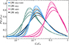Fig. 3. Probability distributions for the normalised anisotropy power spectrum coefficients. Solid curves show the distributions of the multipole ratios for l ∈ {1, 2, 3, 10, 20, 40}, where lighter colours indicate higher multipoles, across four models at the first PTA frequency band. The dashed curve represents the distribution of the sum of the fractional energy density squared of all GW-emitting sources, C∞/C0.

$$\begin{array}{c}\hfill {\displaystyle \underset{l\to \infty }{lim}}\frac{C_l}{C_0}={\displaystyle \sum _i}{r}_i^2\equiv \frac{C_{\infty }}{C_0}.\end{array}$$(17)

This can be shown by considering the fluctuations of their difference:

$$\begin{array}{c}\hfill \frac{C_l}{C_0}-\frac{C_{\infty }}{C_0}=2{\displaystyle \sum _{i>j}}{r}_i{r}_j{P}_l({\widehat{x}}_i·{\widehat{x}}_j).\end{array}$$(18)

The mean of this difference vanishes, ⟨C_l/C₀−C_∞/C₀⟩ = 0, and thus its variance is given by

$$\begin{array}{c}\hfill \langle {(\frac{C_l}{C_0}-\frac{C_{\infty }}{C_0})}^2\rangle =\frac{2}{2l+1}{\displaystyle \sum _{i\ne j}}\langle r_i^2{r}_j^2\rangle .\end{array}$$(19)

The quantities C_l/C₀ and C_∞/C₀ become equivalent when l → ∞ because the variance of their difference vanishes in this limit. Consequently, all higher statistical moments of C_l/C₀ must approach those of C_∞/C₀ when l ≫ 1. This convergence can be intuitively understood by noting that $P_l({\widehat{x}}_i·{\widehat{x}}_j)$ is a rapidly fluctuating function on the sphere when l ≫ 1, and therefore the contributions from different binaries in the second term tend to cancel each other out.

As observed in Fig. 3, the distributions for C_l ≤ 3/C₀ are noticeably broader than that of C_∞/C₀. This agrees with Eq. (16). A good agreement with the distribution of C_∞/C₀ is found at higher multipoles, when l ≥ 10.

3.2. Weak and strong source split

The tail of the distribution at high Ω (9) implies that a handful of strong sources typically dominate the signal even when the total number of sources can be several orders of magnitude larger. As shown in Fig. 1, half of the signal in any NG15 frequency bin originates from at most a few hundred contributions across all models considered here, while the total number of sources can reach around 10⁵. The strongest sources also dominate the anisotropy.

Following Ellis et al. (2024b), Raidal et al. (2024), we modelled the weak and strong sources separately. At a given frequency, we considered a source as strong if its GW signal exceeded a fixed threshold Ω ≥ Ω_thr, specified below. The total luminosity decomposes as

$$\begin{array}{c}\hfill \begin{array}{cc}\hfill \mathrm{\Omega }& ={\mathrm{\Omega }}_S+{\mathrm{\Omega }}_W.\hfill \end{array}\end{array}$$(20)

The strong and weak components, Ω_S and Ω_W, consist of the individual contributions from all strong and weak binaries³:

$$\begin{array}{c}\hfill {\mathrm{\Omega }}_S\equiv {\displaystyle \sum _{i\in I_W}}{\mathrm{\Omega }}_i,{\mathrm{\Omega }}_W\equiv {\displaystyle \sum _{i\in I_S}}{\mathrm{\Omega }}_i.\end{array}$$(21)

Here, I_W and I_S denote the index sets of weak and strong sources, respectively. The multipole ratio (14) then becomes

$$\begin{array}{c}\hfill \begin{array}{cc}\hfill \frac{C_l}{C_0}& ={\displaystyle \sum _{i,j\in I_W}}{r}_i{r}_j{P}_l({\widehat{x}}_i·{\widehat{x}}_i)\hfill \\ \hfill & +2{\displaystyle \sum _{i\in I_W,j\in I_S}}{r}_i{r}_j{P}_l({\widehat{x}}_i·{\widehat{x}}_j)\hfill \\ \hfill & +{\displaystyle \sum _{i,j\in I_S}}{r}_i{r}_j{P}_l({\widehat{x}}_i·{\widehat{x}}_j),\hfill \end{array}\end{array}$$(22)

Averaging over the strengths and sky locations of the weak sources and expanding in weak source luminosity variance gives (see Appendix B)

$$\begin{array}{c}\hfill \begin{array}{cc}\hfill \frac{C_l}{C_0}& \approx \frac{{\overline{\mathrm{\Omega }}}_W^2/N_W}{{({\mathrm{\Omega }}_S+{\overline{\mathrm{\Omega }}}_W)}^2}+{\displaystyle \sum _{i,j\in I_S}}{\overline{r}}_i{\overline{r}}_j{P}_l({\widehat{x}}_{i_S}·{\widehat{x}}_{j_S}),\hfill \end{array}\end{array}$$(23)

where ${\overline{\mathrm{\Omega }}}_W\equiv ⟨{\mathrm{\Omega }}_W⟩$, N_W is the number of weak sources, and we define the rescaled ratio as

$$\begin{array}{c}\hfill {\overline{r}}_i\equiv \frac{{\mathrm{\Omega }}_i}{{\mathrm{\Omega }}_S+{\overline{\mathrm{\Omega }}}_W}.\end{array}$$(24)

This approximation provides the leading contribution when expanding in σ_ΩW²/(Ω_S + Ω_W)², that is, it effectively ignores fluctuations in the luminosity of weak sources. We verified that including the σ_ΩW² correction changes our estimates by at most 1%. In Eq. (23), the individual luminosities of strong sources, and hence their total contribution Ω_S, are random and are modelled using an MC approach. As long as ${\mathrm{\Omega }}_S\gtrsim {\overline{\mathrm{\Omega }}}_W\sqrt{N_S/N_W}$, the dominant contribution arises from the last term in Eq. (23).

4. Results

We chose the threshold strength of a strong source, Ω_thr, such that the number of strong sources was N_S = 50⁴. We generated 10⁵ realisations of the population of strong sources at a given frequency and computed the distributions of the normalised power spectrum coefficients, as described in Sect. 2.

The resulting distributions are shown in Fig. 4. The mean value of the power spectrum coefficients remains constant for ℓ ≥ 1, with the value given by Eq. (15). However, differences in the coefficient distributions exist both between models and also between multipoles. As shown above, the distribution is broadest at the first multipole and, at higher multipoles, it quickly becomes almost independent of l.

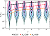Fig. 4. Ratio between the zeroth-order and higher-order coefficients of the GW anisotropy power spectrum. The distributions are obtained from 105 sky realisations at a GW frequency of 1.98 nHz. The medians and means of each distribution are indicated by squares and circles respectively. The dashed black curve represents the NG15 upper bound (Agazie et al. 2023e), while other dashed curves indicate future prospects assuming EPTA-like noise and a 15-year observation time (Depta et al. 2025). The colours of the violin plots correspond to the same models as in Fig. 1.

The magnitude of the anisotropy is partially explained by the number of sources contributing to the GW background for each model, as shown in the left panel of Fig. 1. Environmental effects directly reduce the number of sources in each PTA frequency band, resulting in the smallest number of sources and hence the largest anisotropy. Emission across a range of frequencies due to eccentric orbits result in each binary contributing to multiple frequency bins (including those with primary emission peaks outside the PTA range contributing to the signal). This results in the largest number of contributions and the weakest anisotropy. The combined model is affected by both effects and, consequently, has a number of contributions comparable to the GW-only model and a very similar anisotropy distribution.

The anisotropy of the GW background also depends on the frequency of the measured GWs. This is a combined effect of the change in the number of sources and the strength of GW emission. Sato-Polito & Kamionkowski (2024) shows that the mean anisotropy increases with frequency according to a simple power law at low frequencies, with a model-dependent flattening at higher frequencies. Additional environmental interactions modify the power law and can, for some parameter values, lead to a saddle-shaped curve (see Fig. 4 of Sato-Polito & Kamionkowski 2024). Our results broadly agree with this behaviour, as shown in Fig 5, which displays the intervals containing 68% of the realisations in each frequency band for the four models considered here. Moreover, Fig. 5 shows a distinct separation between the best-fit anisotropies at the lowest frequency bands for the environmental and eccentric models. Although the 68% bands of the eccentric and environmental models for the first multipole moment slightly overlap, they separate at higher multipoles due to the narrowing of their distributions. The GW+env+ecc model and the GW-only model overlap significantly at all frequencies and multipoles.

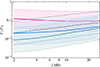Fig. 5. Frequency scaling of the median normalised power spectrum coefficient at l = 1 for each of the four models considered. The shaded areas indicate the 1σ confidence intervals around the median. The colours correspond to the same models as in Fig. 1. The GW-only model is shown with a dashed line for clarity.

5. Discussion

5.1. Prospects for future observations

As shown in Fig. 4, the current NG15 upper bounds on measured anisotropy are sufficiently strong to start constraining environmentally-driven SMBH models, with the mean value of the C₁/C₀ distribution being comparable to the current NG15 bound. However, as the distribution of C₁/C₀ is long-tailed, the most likely value of the distribution remains below the current upper bound. As PTAs add pulsars to their catalogues, these upper bounds on anisotropy will decrease. Possible future bounds for European Pulsar Timing Array (EPTA)-like noise curves and 15-year observational times derived in Depta et al. (2025) are also shown in Fig. 4 for different numbers of pulsars observed. For N_p = 200, the GW+env model of circular binaries can be almost fully excluded in the case of non-measurement. The anisotropy of circular GW emission only and eccentric SMBH binary models are likely to be probed only at much larger numbers of pulsars, N_p ≥ 500. However, the prospects improve with increases in the precision of the timing measurements. As shown in Depta et al. (2025), the prospective upper bounds for C_l/C₀ with Square Kilometre Array (SKA)-like noise for the same number of pulsars are almost an order of magnitude stronger than with EPTA-like noise.

5.2. Spectral fluctuations and resolvable sources

GW backgrounds dominated by a few sources tend to be more anisotropic than those dominated by many sources. This results in a positive correlation between anisotropy and spectral fluctuations. A naive quantitative estimate can be made by noting that, with N GW sources, the average over the sky locations satisfies ${⟨C_l/C_0⟩}_{\widehat{x}}=C_{\infty }/C_0\ge 1/N$, and that this inequality is saturated when all sources are equally loud, r_i = 1/N. Without the sky average, downward fluctuations are possible due to cancellations between the Legendre polynomials in (14). This inequality can be further refined to find the lower and upper bounds,

$$\begin{array}{c}\hfill r_{\max }\ge \frac{C_{\infty }}{C_0}\ge \frac{p^2}{N_p},\end{array}$$(25)

where N_p is the number of loudest sources contributing the fraction p to the signal and r_max is the fractional strength of the loudest signal. The upper bound follows from (17), noting that anisotropy is maximised if the signal consists of N = 1/r_max sources with maximal strength r_max. When considering only the strongest source, the lower bound reads C_∞/C₀ ≥ r_max² since N_p = 1 and p = r_max.

The lower bound quantifies the intuitio n that the anisotropy is large when the signal is dominated by a few strong sources. The upper bound indicates that a large anisotropy implies the presence of sources that contribute a significant fraction to the signal. Importantly, Fig. 3 shows a non-vanishing probability that C_∞/C₀ is practically one, in which case a single source must completely dominate the GW signal.

To account for the sky locations of the SMBH binaries in C_l/C₀ in specific realisations of the SMBH binary population, requires numerical methods. Figure 6 shows the relation between the energy content of the strongest individual GW source and the level of the dipole, C₁/C₀, obtained from 10⁴ realisations of the SMBH population, at both f = 1.98 nHz and f = 27.68 nHz. The darker and lighter shaded contours contain 68% and 95% of the realisations, respectively. There is a clear trend showing that SMBH populations with the loudest binaries tend to be more anisotropic. When Ω_max ≈ Ω_tot or r_max ≈ 1, we find C_l/C₀ ≈ (Ω_max/Ω_tot)² ≡ r_max², suggesting that the anisotropy is dominated by a single source in these realisations.

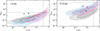Fig. 6. Gravitational wave (GW) contribution from the loudest binary versus the first multipole in frequency bins at f = 1.98 nHz (left) and f = 27.68 nHz (right). The darker and lighter shaded contours indicate regions containing 68% and 95% of the realisations, respectively. Colours correspond to the same models as in Fig. 1. The star marks the median of (Ωtot, C1/C0). The dashed grey vertical and horizontal lines denote the current NG15 upper bound on C1/C0 (Agazie et al. 2023e) and the individual SMBH binary detection (Agazie et al. 2023a), respectively.

The median realisations of the total GW signal and C₁/C₀ are shown by stars in Fig. 6 (corresponding to the squares in Fig. 4). Thus, Ω_max values comparable to or higher than the star likely correspond to realisations in which the strongest binary contributes a sizeable fraction of the GW signal and is responsible for an upward spectral fluctuation at that frequency. This is unlikely unless the stars are within the corresponding shaded areas, that is, at higher frequencies or for models involving environmental effects.

The dependence of these correlations on the GW frequency is non-trivial. However, the general characteristics of the correlations reflect the behaviour seen in Figs. 5 and 1: for the circular environmental model, the number of loudest binaries remains constant whilst it decreases for the other models. The total amplitude of the GW signal, whose median value is indicated by the star, increases with frequency for all models, although the growth is mild in the GW-only model. When the number of strong sources decreases, the loudest contribution, Ω_max, increases in magnitude and strength relative to the other sources for all models. This shifts the contours towards larger Ω_max and increases anisotropy, seen as a shift to higher values of C₁/C₀ in the contours.

The dashed lines in Fig. 6 indicate the NG15 constraints on C₁/C₀ (Agazie et al. 2023e) and on the individual detection of a SMBH binary (Agazie et al. 2023a). Currently, the non-observation of both quantities mostly excludes the high-amplitude end of spectral and anisotropy fluctuations.

5.3. Including cosmological backgrounds

The PTA GW background may not arise purely from SMBH mergers, but could also contain a cosmological component, Ω_CGWB(f), originating from the primordial Universe. Many cosmological models can fit the recent PTA data as well as, or slightly better than, SMBH models (Ellis et al. 2024a). In such cases, the GW spectrum is decomposed as

$$\begin{array}{c}\hfill \mathrm{\Omega }(f)={\mathrm{\Omega }}_{\mathrm{SMBH}}(f)+{\mathrm{\Omega }}_{\mathrm{CGWB}}(f).\end{array}$$(26)

In contrast to the GW background from SMBHs, Ω_SMBH(f), we expect Ω_SMBH(f) to be isotropic and smooth, that is, without notable spectral fluctuations.

To accommodate this background into the formalism above, the relative contribution from a single binary must be rescaled (as above, we drop the explicit frequency dependence), giving

$$\begin{array}{c}\hfill r_i=\frac{{\mathrm{\Omega }}_i}{{\mathrm{\Omega }}_{\mathrm{SMBH}}+{\mathrm{\Omega }}_{\mathrm{CGWB}}}\equiv r_{i,\mathrm{BH}}{r}_{\mathrm{SMBH}},\end{array}$$(27)

where r_i,BH ≡ Ω_i/Ω_SMBH is the relative strength from an individual binary compared to the GW signal from all binaries, and r_SMBH ≡ Ω_SMBH/(Ω_SMBH + Ω_CGWB) is the fraction of the total signal from binaries. The anisotropy for a particular realisation of the SMBH population can then be described by Eq. (14).

Homogeneous cosmological backgrounds with negligible statistical fluctuations can be easily included in the approach summarised by Eq. (23), in which binary sources are split into weak and strong subsets. To include the cosmological background, the shift

$$\begin{array}{c}\hfill {\overline{\mathrm{\Omega }}}_W\to {\overline{\mathrm{\Omega }}}_W+{\mathrm{\Omega }}_{\mathrm{CGWB}}\end{array}$$(28)

should be performed only in the denominator Eqs. (23) and (24). The numerator in Eq. (23) gives the contribution to the variance from weak binaries and is not affected by the cosmological background. Nevertheless, Eq. (23) demonstrates that there is a degeneracy between the strength of cosmological GW backgrounds, Ω_CGWB, and the leading characteristics of the weak SMBH binary populations, ${\overline{\mathrm{\Omega }}}_W$ and N_W.

A rough estimate of the contribution from a cosmological GW background can be obtained by replacing the last term in Eq. (27) by its average, r_i ≈ r_i,BH ⟨r_SMBH⟩. In that case, we find that compared to the SMBH-only case, the anisotropy is reduced by a factor of ⟨r_SMBH⟩², that is

$$\begin{array}{c}\hfill \frac{C_{l\ge 1}}{C_0}\approx {\frac{C_{l\ge 1}}{C_0}|}_{{\mathrm{\Omega }}_{\mathrm{CGWB}}=0}{⟨r_{\mathrm{SMBH}}⟩}^2.\end{array}$$(29)

Statistically, this approximation amounts to neglecting the correlations between r_i,BH and r_SMBH. However, as r_SMBH tends to have a heavy tail created mainly due to the loudest SMBH, that is, the largest r_i,BH, we expect that such correlations can have a sizeable 𝒪(1) effect on C_l/C₀. Thus, the approximate scaling in Eq. (29) can provide an order-of-magnitude estimate at best.

A mixed signal from SMBHs and cosmological sources would be harder to probe using anisotropies due to uncertainty in the proportion of the signal coming from SMBHs and difficulty in resolving lower values of the anisotropy power spectrum coefficients.

6. Conclusions

We studied the statistical properties of the anisotropy of GW backgrounds from SMBHs. We derived the distributions of the (normalised) anisotropy power spectrum coefficients, C_l/C₀, and characterised their dependence on multipole number and frequency. We show that these distributions are widest at l = 1, and, assuming statistical isotropy, tend towards an l-independent distribution that is fully characterised by the distribution of GW luminosities of the SMBH binaries.

We investigated the anisotropy distributions of four models of SMBH binary evolution in benchmark cases found to best fit the GW background spectrum inferred from the NANOGrav 15-year measurements. The magnitude of the predicted anisotropies largely depends on the number of strong sources contributing to the GW background at a given frequency. The smallest anisotropy is given by a model with eccentric binaries (which has the largest number of contributions to a given frequency bin) and the largest anisotropy by a model describing circular binaries affected by the environment (where the GW signal is typically dominated by less than ten sources).

We compared the predicted anisotropies with the current upper bounds, finding that the model incorporating only environmental effects is in a mild tension with the bounds. We also compared these to projected upper bounds for future measurements with expanded pulsar catalogues. A catalogue of N_p = 200 pulsars and a 15 year measurement time would be sufficient to nearly fully exclude the best fit of the pure environmental effect and would probe the anisotropies in models with circular binaries evolving only via GW emission and the model combining eccentric binaries and environmental effects. The sensitivity required to investigate the anisotropy generated by eccentric binaries without environmental effects will only be reached with experiments having N_p ≥ 500. These prospects hold under the assumption that the GW background originates purely from SMBH binaries. For signals of mixed cosmological and astrophysical origin, the anisotropy is reduced.

Large upward fluctuations in the GW amplitude are typically accompanied by heightened anisotropy. We quantified the relation between anisotropy and the GW luminosity of the strongest source. Because this relation varies from model to model, determining the correlation between spectral fluctuations and anisotropy opens new avenues for SMBH model discrimination.

Acknowledgments

This work was supported by the Estonian Research Council grants PRG803, PSG869, RVTT3 and RVTT7 and the Center of Excellence program TK202. The work of V.V. was partially funded by the European Union’s Horizon Europe research and innovation program under the Marie Skłodowska-Curie grant agreement No. 101065736.

References

Appendix A: Modelling eccentricity and environmental effects

A general eccentric binary emits GWs in several harmonic modes with the power emitted in the n-th harmonic being (Peters & Mathews 1963)

$$\begin{array}{c}\hfill \begin{array}{cc}\hfill \frac{\mathrm{d}{E}_n}{\mathrm{d}{t}_r}& =\frac{32}{5}{(2\pi \mathcal{M}{f}_{\mathrm{b}})}^{10/3}{g}_n(e)\equiv \frac{\mathrm{d}{E}_c}{\mathrm{d}{t}_r}{g}_n(e),\hfill \end{array}\end{array}$$(A.1)

where ℳ denotes the chirp mass, f_b the orbital frequency and z the redshift of the binary, and dE_c/dt_r is the power emitted by a circular binary with the above binary parameters. The observer frame time t is related to the time t_r in the rest frame of the binary by dt = (1 + z)dt_r. The relative power radiated in the n-th harmonic is

$$\begin{array}{c}\hfill \begin{array}{cc}& g_n(e)=\frac{n^4}{32}[\frac{4}{3n^2}{J}_n^2(ne)+(J_{n-2}(ne)-2e{J}_{n-1}(ne)\hfill \\ \hfill & +\frac{2}{n}{J}_n(ne)+2e{J}_{n+1}(ne)-J_{n+2}(ne){)}^2\hfill \\ \hfill & +(1-e^2)(J_{n-2}(ne)-2J_n(ne)+J_{n+2}(ne){)}^2],\hfill \end{array}\end{array}$$(A.2)

where J_n are the n-th Bessel functions of the first kind. Note that, for circular binaries, g_n(0) = δ_2, n.

The total power emitted by a binary across all frequencies is

$$\begin{array}{c}\hfill \frac{\mathrm{d}{E}_{\mathrm{GW}}}{\mathrm{d}{t}_r}=\frac{\mathrm{d}{E}_c}{\mathrm{d}{t}_r}\mathcal{F}(e),\end{array}$$(A.3)

where

$$\begin{array}{c}\hfill \mathcal{F}(e)={\displaystyle \sum _{n=1}^{\infty }}{g}_n(e)=\frac{1+73/24e^2+37/96e^4}{{(1-e^2)}^{7/2}}.\end{array}$$(A.4)

Note that ℱ(0) = 1.

The orbital dynamics of a black hole binary is given by the evolution of its orbital frequency and eccentricity (Peters & Mathews 1963)

$$\begin{array}{c}\hfill \begin{array}{cc}\hfill \frac{\mathrm{d}ln{f}_{\mathrm{b}}}{\mathrm{d}{t}_r}& =\frac{96}{5}{\mathcal{M}}^{5/3}{(2\pi f_{\mathrm{b}})}^{8/3}\mathcal{F}(e),\hfill \\ \hfill \frac{\mathrm{d}e}{\mathrm{d}{t}_r}& =-\frac{1}{15}{\mathcal{M}}^{5/3}{(2\pi f_{\mathrm{b}})}^{8/3}\mathcal{G}(e),\hfill \end{array}\end{array}$$(A.5)

where

$$\begin{array}{c}\hfill \mathcal{G}(e)=\frac{304e+121e^3}{{(1-e^2)}^{5/2}}.\end{array}$$(A.6)

From this, the observed residence time of a binary at orbital frequency f_b is

$$\begin{array}{c}\hfill \begin{array}{cc}\hfill \frac{\mathrm{d}t}{\mathrm{d}ln{f}_{\mathrm{b}}}& =\frac{5}{96}\frac{1+z}{{\mathcal{M}}^{5/3}}{(2\pi f_{\mathrm{b}})}^{-8/3}\frac{1}{\mathcal{F}(e)}\equiv \frac{2}{3}{t}_{\mathrm{GW}}\hfill \end{array}\end{array}$$(A.7)

where t_GW ≡ |E|/Ė_GW is the characteristic timescale of energy loss through GW emission. The factor 1 + z arises when converting the binary rest frame time t_r to the time t in the observer frame.

Following Raidal et al. (2024), we model the binary eccentricities by fixing the distribution of e at the lowest NG15 frequency bin. We consider a power-law distribution P(e) = (γ + 1)e^γ and trade γ for the mean initial eccentricity, ⟨e⟩_2 nHz = (1 + γ)/(2 + γ), which is the only free parameter of our eccentricity model.

The residence time can be further modified due to interactions between the SMBH binary and its environment. Their exact impact is unknown and, for the sake of simplicity and generality, we introduce them via the environmental timescale t_env ≡ |E|/Ė_env of energy loss, for which will adapt the power-law ansatz (Ellis et al. 2024b),

$$\begin{array}{c}\hfill t_{\mathrm{env}}=t_{\mathrm{GW}}{\left(\frac{2f_b}{f_{\mathrm{GW}}}\right)}^{\alpha },f_{\mathrm{GW}}=f_{\mathrm{ref}}{\left(\frac{\mathcal{M}}{{10}^9{M}_{\odot }}\right)}^{\beta },\end{array}$$(A.8)

and fix α = 8/3 and β = 5/8 so that f_ref is the only free parameter of the model. These values correspond to gas infall driven binary evolution (Begelman et al. 1980). Note that since t_GW ∝ f^−8/3, the chosen value of α implies that t_env is frequency independent. Environmental interactions lead to the shortening of the residence time of a binary as given by

$$\begin{array}{c}\hfill \begin{array}{cc}\hfill \frac{\mathrm{d}t}{\mathrm{d}ln{f}_{\mathrm{b}}}& =\frac{2}{3}{t}_{\mathrm{GW}}{[1+\frac{t_{\mathrm{GW}}}{t_{\mathrm{env}}}]}^{-1}\hfill \end{array}\end{array}$$(A.9)

The orbital frequency evolution of the binary eccentricity is affected in a similar manner (Raidal et al. 2024),

$$\begin{array}{c}\hfill \frac{\mathrm{d}e}{\mathrm{d}ln{f}_{\mathrm{b}}}=-\frac{1}{288}\frac{\mathcal{G}(e)}{\mathcal{F}(e)}{[1+\frac{t_{\mathrm{GW}}}{t_{\mathrm{env}}}]}^{-1}.\end{array}$$(A.10)

Appendix B: Statistics of C_l/C₀

Here we list some of the identities used in the derivation of the results in the main text.

The angular averages involve only the Legendre polynomials. Most of the results stem from the identity

$$\begin{array}{c}\hfill {\displaystyle \int \frac{\mathrm{d}{\mathrm{\Omega }}_i}{4\pi }}{P}_l({\widehat{x}}_m·{\widehat{x}}_i)P_{l^{\prime }}({\widehat{x}}_i·{\widehat{x}}_n)=\frac{{\delta }_{l{l}^{\prime }}}{2l+1}{P}_l({\widehat{x}}_m·{\widehat{x}}_m)\end{array}$$(B.1)

For l > 0 we have that

$$\begin{array}{c}\hfill \begin{array}{cc}\hfill {⟨P_l({\widehat{x}}_i·{\widehat{x}}_j)⟩}_{{\widehat{x}}_i}& =0,\hfill \\ \hfill ⟨P_l({\widehat{x}}_i·{\widehat{x}}_j)P_l({\widehat{x}}_i·{\widehat{x}}_m)⟩& ={\delta }_{\mathit{ij}}{\delta }_{\mathit{mn}}\hfill \\ \hfill & +\frac{{\delta }_{\mathit{im}}{\delta }_{\mathit{jn}}+{\delta }_{\mathit{in}}{\delta }_{\mathit{jm}}-2{\delta }_{\mathit{ij}}{\delta }_{\mathit{mn}}}{2l+1},,\hfill \end{array}\end{array}$$

where the first average is taken only over ${\widehat{x}}_i$.

To compute higher moments, we will split C_l/C₀ into two pieces

$$\begin{array}{c}\hfill \frac{C_l}{C_0}={\displaystyle \sum _i}{r}_i^2+{\displaystyle \sum _{i\ne j}}{r}_i{r}_j{P}_l({\widehat{x}}_i·{\widehat{x}}_j)\equiv \frac{C_{\infty }}{C_0}+{\mathrm{\Delta }}_l\end{array}$$(B.2)

which can be used to study specific statistical properties of C_l/C₀. Importantly, C_∞/C₀ does not depend on the spatial distribution. It is fully determined by the distribution of the signal’s relative loudness. The following expectation values can be estimated

$$\begin{array}{c}\hfill \begin{array}{cc}\hfill ⟨{\mathrm{\Delta }}_l⟩& =\langle {\mathrm{\Delta }}_l\frac{C_{\infty }}{C_0}\rangle =0,\hfill \\ \hfill ⟨{\mathrm{\Delta }}_l^2⟩& ={\displaystyle \sum _{i\ne j,m\ne n}}⟨r_i{r}_j{r}_m{r}_n⟩⟨P_l({\widehat{x}}_i·{\widehat{x}}_j)P_l({\widehat{x}}_m·{\widehat{x}}_n)⟩,\hfill \\ \hfill & =\frac{2}{2l+1}{\displaystyle \sum _{i\ne j}}⟨r_i^2{r}_j^2⟩,\hfill \\ \hfill \langle \frac{C_{\infty }}{C_0}\rangle & ={\displaystyle \sum _i}\langle r_i^2\rangle ,\hfill \\ \hfill \langle {\left(\frac{C_{\infty }}{C_0}\right)}^2\rangle & ={\displaystyle \sum _i}\langle r_i^4\rangle +{\displaystyle \sum _{i\ne j}}\langle r_i^2{r}_j^2\rangle ,\hfill \end{array}\end{array}$$(B.3)

and thus

$$\begin{array}{c}\hfill \begin{array}{cc}\hfill \langle C_l/C_0\rangle & =\langle C_{\infty }/C_0\rangle ,\hfill \\ \hfill {\sigma }_{C_l/C_0}^2& ={\sigma }_{C_{\infty }/C_0}^2+{\sigma }_{{\mathrm{\Delta }}_l}^2\hfill \end{array}\end{array}$$(B.4)

confirming the expressions in Sec. 3.

Since all r_i are statistically identical but not independent, then it’s sufficient to the expectation values related to a single or a few sources, such as, ⟨r₁^m⟩ , ⟨r₁^mr₂ⁿ⟩ , …,  using which we can eliminate the sums in Eq. (B.3):

$$\begin{array}{c}\hfill \begin{array}{cc}\hfill ⟨{\mathrm{\Delta }}_l^2⟩& =\frac{2N_{\mathrm{b}}(N_{\mathrm{b}}-1)}{2l+1}⟨r_1^2{r}_2^2⟩,\hfill \\ \hfill \langle \frac{C_{\infty }}{C_0}\rangle & =N_{\mathrm{b}}\langle r_1^2\rangle ,\hfill \\ \hfill \langle {\left(\frac{C_{\infty }}{C_0}\right)}^2\rangle & =N_{\mathrm{b}}\langle r_1^4\rangle +N_{\mathrm{b}}(N_{\mathrm{b}}-1)\langle r_1^2{r}_2^2\rangle .\hfill \end{array}\end{array}$$(B.5)

Let us now consider the average over the weak sources of Eq. (22), which we express here as

$$\begin{array}{c}\hfill C_l/C_0=I_W+I_{\mathit{WS}}+I_S,\end{array}$$

where

$$\begin{array}{c}\hfill \begin{array}{cc}\hfill {\mathcal{I}}_W& \equiv {\displaystyle \sum _{i,j\in I_W}}{r}_i{r}_j{P}_l({\widehat{x}}_i·{\widehat{x}}_i)\hfill \\ \hfill {\mathcal{I}}_{\mathit{WS}}& \equiv 2{\displaystyle \sum _{i\in I_W,j\in I_S}}{r}_i{r}_j{P}_l({\widehat{x}}_i·{\widehat{x}}_j)\hfill \\ \hfill {\mathcal{I}}_S& \equiv {\displaystyle \sum _{i,j\in I_S}}{r}_i{r}_j{P}_l({\widehat{x}}_i·{\widehat{x}}_j)\hfill \end{array}\end{array}$$(B.6)

The mean of the central term vanishes, ⟨ℐ_WS⟩_W = 0 because the positions of the weak sources are not correlated with the strong ones (the subindex W denotes averaging over weak sources only).

The only relevant terms are thus ℐ_S and ℐ_W which we’ll compute up to the order σ_ΩW². To simplify the derivation, we’ll denote

$$\begin{array}{c}\hfill \begin{array}{cc}\hfill \delta {\mathrm{\Omega }}_i& \equiv {\mathrm{\Omega }}_i-{\overline{\mathrm{\Omega }}}_1,{\mathrm{\Omega }}_{W,i}\equiv {\mathrm{\Omega }}_W-\delta {\mathrm{\Omega }}_i,\hfill \end{array}\end{array}$$(B.7)

where ${\overline{\mathrm{\Omega }}}_1\equiv {⟨{\mathrm{\Omega }}_i⟩}_W$ is the average of a single source. Ω_W, i is the total strength of weak sources with the i-th source replaced by its average. Since Ω_i are independent, then so are Ω_W, i and δΩ_i. We will consider an expansion in δΩ_i as it is expected to be small compared to both Ω_S and Ω_W.

Moreover, ℐ_W is simplified because ${⟨P_l({\widehat{x}}_i·{\widehat{x}}_j)⟩}_W={\delta }_{\mathit{ij}}$ so that

$$\begin{array}{c}\hfill \begin{array}{cc}\hfill {\langle {\mathcal{I}}_W\rangle }_W& ={\displaystyle \sum _{i\in I_W}}{\langle r_i^2\rangle }_W={\displaystyle \sum _{i\in I_W}}{\langle \frac{{\mathrm{\Omega }}_i^2}{{({\mathrm{\Omega }}_S+{\mathrm{\Omega }}_W)}^2}\rangle }_W={\displaystyle \sum _{i\in I_W}}{\langle \frac{{({\overline{\mathrm{\Omega }}}_1+\delta {\mathrm{\Omega }}_i)}^2}{{({\mathrm{\Omega }}_S+{\mathrm{\Omega }}_{W,i}+\delta {\mathrm{\Omega }}_i)}^2}\rangle }_W\hfill \\ \hfill & ={\displaystyle \sum _{i\in I_W}}{\langle \frac{{\overline{\mathrm{\Omega }}}_1^2+⟨\delta {\mathrm{\Omega }}_i^2⟩}{{({\mathrm{\Omega }}_S+{\mathrm{\Omega }}_{W,i})}^2}-\frac{4{\overline{\mathrm{\Omega }}}_1⟨\delta {\mathrm{\Omega }}_i^2⟩}{{({\mathrm{\Omega }}_S+{\mathrm{\Omega }}_{W,i})}^3}+\frac{3{\overline{\mathrm{\Omega }}}_1^2⟨\delta {\mathrm{\Omega }}_i^2⟩}{{({\mathrm{\Omega }}_S+{\mathrm{\Omega }}_{W,i})}^4}+\mathcal{O}(\delta {\mathrm{\Omega }}_i^3)\rangle }_W\hfill \\ \hfill & =\frac{{\overline{\mathrm{\Omega }}}_W^2{N}_W^{-1}}{{({\mathrm{\Omega }}_S+{\overline{\mathrm{\Omega }}}_W)}^2}+\frac{{\sigma }_{{\mathrm{\Omega }}_W}^2}{{({\mathrm{\Omega }}_S+{\overline{\mathrm{\Omega }}}_W)}^2}[1-\frac{4{\overline{\mathrm{\Omega }}}_W{N}_W^{-1}}{{\mathrm{\Omega }}_S+{\overline{\mathrm{\Omega }}}_W}+\frac{3{\overline{\mathrm{\Omega }}}_W^2{N}_W^{-1}}{{({\mathrm{\Omega }}_S+{\overline{\mathrm{\Omega }}}_W)}^2}]+\mathcal{O}({\sigma }_{{\mathrm{\Omega }}_W}^3),\hfill \end{array}\end{array}$$(B.8)

where we dropped terms linear in δΩ_i as their averages vanish. We also use ${\overline{\mathrm{\Omega }}}_1={\overline{\mathrm{\Omega }}}_W/N$ and ⟨δΩ_i²⟩=σ_ΩW²/N_W, where N_W is the number of weak sources. In the last step, we estimated the average of the denominator

$$\begin{array}{c}\hfill {\langle \frac{1}{{({\mathrm{\Omega }}_S+{\mathrm{\Omega }}_W)}^n}\rangle }_W=\frac{1}{{({\mathrm{\Omega }}_S+{\overline{\mathrm{\Omega }}}_W)}^n}+\frac{n(n+1)}{2}\frac{{\sigma }_{{\mathrm{\Omega }}_W}^2}{{({\mathrm{\Omega }}_S+{\overline{\mathrm{\Omega }}}_W)}^{n+2}}+\mathcal{O}({\sigma }_{{\mathrm{\Omega }}_W}^4)\end{array}$$(B.9)

by expanding in $\delta {\mathrm{\Omega }}_W\equiv {\mathrm{\Omega }}_W-{\overline{\mathrm{\Omega }}}_W$. Note that $⟨{\mathrm{\Omega }}_{W,i}⟩=⟨{\mathrm{\Omega }}_W⟩\equiv {\overline{\mathrm{\Omega }}}_W$ and σ_ΩW, i² = (1 − N_W⁻¹)σ_ΩW⁴.

A similar procedure gives

$$\begin{array}{c}\hfill \begin{array}{cc}\hfill {\langle {\mathcal{I}}_S\rangle }_W& ={\langle \frac{1}{{({\mathrm{\Omega }}_S+{\mathrm{\Omega }}_W)}^2}\rangle }_W{\displaystyle \sum _{i,j\in I_S}}{\mathrm{\Omega }}_i{\mathrm{\Omega }}_j{P}_l({\widehat{x}}_i·{\widehat{x}}_j)\hfill \end{array}\end{array}$$(B.10)

where average is given by (B.9).

The approximation given in Eq. (22) for the weak-strong split is obtained by dropping the 𝒪(σ_ΩW²) terms. Including the 𝒪(σ_ΩW²) correction affects the results by less than 1% with N_S = 50 strong sources. The corrections would be further suppressed when Ω_W ≪ Ω_S, which we do not require.

We also note that we have estimated the corrections when averaging over weak sources due to spectral fluctuations caused by weak sources. However, the averaging procedure itself is an approximation and we expect that the corrections to the width of the distribution of C_l/C₀ are of the order σ_ΩW². The heavy non-Gaussian tail of the Ω distribution guarantees that such corrections are negligible, that is, the tail can be fully modelled by the strong sources.

All Figures

Fig. 1. Gravitational wave (GW) characteristics of the SMBH binary population for four different SMBH models: purely GW driven inspirals (GW only), inspirals with environmental effects (GW+env), inspirals of eccentric SMBH binaries (GW+ecc), and inspirals of eccentric SMBH binaries with environmental effects (GW+ecc+env). Left panel: Median (solid line) and mean (dashed line) number of the strongest sources contributing half the signal at each PTA frequency band. Middle panel: Distributions of contributions from individual binaries at 1.98 nHz (solid lines) and 27.68 nHz (dashed lines). Right panel: Distributions of the GW spectra in the n × 1.98 nHz frequency bins compared to NANOGrav 15-year data (yellow violin plots).

In the text

	Fig. 2. Typical realisation of the strongest binaries contributing 50% of the GW signal in the 1.98 nHz frequency bin for the GW+env (left), GW+ecc+env (middle-left), GW-only (middle-right), and GW+ecc (right) models. The colour and size of the binary markers indicate the relative magnitude of GW energy emitted by each binary.
In the text

Fig. 3. Probability distributions for the normalised anisotropy power spectrum coefficients. Solid curves show the distributions of the multipole ratios for l ∈ {1, 2, 3, 10, 20, 40}, where lighter colours indicate higher multipoles, across four models at the first PTA frequency band. The dashed curve represents the distribution of the sum of the fractional energy density squared of all GW-emitting sources, C∞/C0.

In the text

Fig. 4. Ratio between the zeroth-order and higher-order coefficients of the GW anisotropy power spectrum. The distributions are obtained from 105 sky realisations at a GW frequency of 1.98 nHz. The medians and means of each distribution are indicated by squares and circles respectively. The dashed black curve represents the NG15 upper bound (Agazie et al. 2023e), while other dashed curves indicate future prospects assuming EPTA-like noise and a 15-year observation time (Depta et al. 2025). The colours of the violin plots correspond to the same models as in Fig. 1.

In the text

	Fig. 5. Frequency scaling of the median normalised power spectrum coefficient at l = 1 for each of the four models considered. The shaded areas indicate the 1σ confidence intervals around the median. The colours correspond to the same models as in Fig. 1. The GW-only model is shown with a dashed line for clarity.
In the text

Fig. 6. Gravitational wave (GW) contribution from the loudest binary versus the first multipole in frequency bins at f = 1.98 nHz (left) and f = 27.68 nHz (right). The darker and lighter shaded contours indicate regions containing 68% and 95% of the realisations, respectively. Colours correspond to the same models as in Fig. 1. The star marks the median of (Ωtot, C1/C0). The dashed grey vertical and horizontal lines denote the current NG15 upper bound on C1/C0 (Agazie et al. 2023e) and the individual SMBH binary detection (Agazie et al. 2023a), respectively.

In the text

References

- Afzal, A., Agazie, G., Anumarlapudi, A., et al. 2023, ApJ, 951, L11 [NASA ADS] [CrossRef] [Google Scholar]
- Agazie, G., Anumarlapudi, A., Archibald, A. M., et al. 2023a, ApJ, 951, L50 [NASA ADS] [CrossRef] [Google Scholar]
- Agazie, G., Anumarlapudi, A., Archibald, A. M., et al. 2023b, ApJ, 952, L37 [NASA ADS] [CrossRef] [Google Scholar]
- Agazie, G., Anumarlapudi, A., Archibald, A. M., et al. 2023c, ApJ, 951, L8 [NASA ADS] [CrossRef] [Google Scholar]
- Agazie, G., Alam, M. F., Anumarlapudi, A., et al. 2023d, ApJ, 951, L9 [CrossRef] [Google Scholar]
- Agazie, G., Anumarlapudi, A., Archibald, A. M., et al. 2023e, ApJ, 956, L3 [Google Scholar]
- Allen, B., Agarwal, D., Romano, J. D., & Valtolina, S. 2024, PRD, 110, 123507 [Google Scholar]
- Alonso-Álvarez, G., Cline, J. M., & Dewar, C. 2024, PRL, 133, 021401 [Google Scholar]
- Antoniadis, J., Arumugam, P., Arumugam, S., et al. 2023a, A&A, 678, A48 [NASA ADS] [CrossRef] [EDP Sciences] [Google Scholar]
- Antoniadis, J., Arumugam, P., Arumugam, S., et al. 2023b, A&A, 678, A50 [CrossRef] [EDP Sciences] [Google Scholar]
- Antoniadis, J., Arumugam, P., Arumugam, S., et al. 2024, A&A, 685, A94 [NASA ADS] [CrossRef] [EDP Sciences] [Google Scholar]
- Begelman, M. C., Blandford, R. D., & Rees, M. J. 1980, Nature, 287, 307 [Google Scholar]
- Bi, Y.-C., Wu, Y.-M., Chen, Z.-C., & Huang, Q.-G. 2023, Sci. China Phys. Mech. Astron., 66, 120402 [NASA ADS] [CrossRef] [Google Scholar]
- Bond, J. R., Cole, S., Efstathiou, G., & Kaiser, N. 1991, ApJ, 379, 440 [NASA ADS] [CrossRef] [Google Scholar]
- Bonetti, M., Sesana, A., Barausse, E., & Haardt, F. 2018, MNRAS, 477, 2599 [NASA ADS] [CrossRef] [Google Scholar]
- Chen, S., Middleton, H., Sesana, A., Del Pozzo, W., & Vecchio, A. 2017a, MNRAS, 468, 404 [NASA ADS] [CrossRef] [Google Scholar]
- Chen, S., Sesana, A., & Del Pozzo, W. 2017b, MNRAS, 470, 1738 [CrossRef] [Google Scholar]
- Chen, Y., Yu, Q., & Lu, Y. 2020, ApJ, 897, 86 [Google Scholar]
- Chen, Y., Daniel, M., D’Orazio, D. J., et al. 2024, ArXiv e-prints [arXiv:2411.05906] [Google Scholar]
- Cornish, N. J., & van Haasteren, R. 2014, ArXiv e-prints [arXiv:1406.4511] [Google Scholar]
- Cruz, N. M. J., Malhotra, A., Tasinato, G., & Zavala, I. 2024a, PRD, 110, 063526 [Google Scholar]
- Cruz, N. M. J., Malhotra, A., Tasinato, G., & Zavala, I. 2024b, PRD, 110, 103505 [Google Scholar]
- Depta, P. F., Domcke, V., Franciolini, G., & Pieroni, M. 2025, PRD, 111, 083039 [Google Scholar]
- Ellis, J., Fairbairn, M., Hütsi, G., et al. 2023, A&A, 676, A38 [NASA ADS] [CrossRef] [EDP Sciences] [Google Scholar]
- Ellis, J., Fairbairn, M., Franciolini, G., et al. 2024a, PRD, 109, 023522 [Google Scholar]
- Ellis, J., Fairbairn, M., Hütsi, G., et al. 2024b, PRD, 109, L021302 [Google Scholar]
- Ellis, J., Fairbairn, M., Hütsi, G., et al. 2024c, A&A, 691, A270 [NASA ADS] [CrossRef] [EDP Sciences] [Google Scholar]
- Enoki, M., & Nagashima, M. 2007, PTP, 117, 241 [Google Scholar]
- Fastidio, F., Gualandris, A., Sesana, A., Bortolas, E., & Dehnen, W. 2024, MNRAS, 532, 295 [NASA ADS] [CrossRef] [Google Scholar]
- Figueroa, D. G., Pieroni, M., Ricciardone, A., & Simakachorn, P. 2024, PRL, 132, 171002 [Google Scholar]
- Gardiner, E. C., Kelley, L. Z., Lemke, A.-M., & Mitridate, A. 2024, ApJ, 965, 164 [NASA ADS] [CrossRef] [Google Scholar]
- Girelli, G., Pozzetti, L., Bolzonella, M., et al. 2020, A&A, 634, A135 [NASA ADS] [CrossRef] [EDP Sciences] [Google Scholar]
- Hellings, R.w., & Downs, G. S. 1983, ApJ, 265, L39 [NASA ADS] [CrossRef] [Google Scholar]
- Hotinli, S. C., Kamionkowski, M., & Jaffe, A. H. 2019, OJAp, 2, 8 [Google Scholar]
- Kocsis, B., & Sesana, A. 2011, MNRAS, 411, 1467 [NASA ADS] [CrossRef] [Google Scholar]
- Lacey, C., & Cole, S. 1993, MNRAS, 262, 627 [NASA ADS] [CrossRef] [Google Scholar]
- Lemke, A.-M., Mitridate, A., & Gersbach, K. A. 2025, PRD, 111, 063068 [Google Scholar]
- Mingarelli, C. M. F., Sidery, T., Mandel, I., & Vecchio, A. 2013, PRD, 88, 062005 [Google Scholar]
- Peters, P. C., & Mathews, J. 1963, Phys. Rev., 131, 435 [Google Scholar]
- Pol, N., Taylor, S. R., & Romano, J. D. 2022, ApJ, 940, 173 [NASA ADS] [CrossRef] [Google Scholar]
- Press, W. H., & Schechter, P. 1974, ApJ, 187, 425 [Google Scholar]
- Raidal, J., Urrutia, J., Vaskonen, V., & Veermäe, H. 2024, A&A, 691, A212 [NASA ADS] [CrossRef] [EDP Sciences] [Google Scholar]
- Reardon, D. J., Zic, A., Shannon, R. M., et al. 2023a, ApJ, 951, L6 [NASA ADS] [CrossRef] [Google Scholar]
- Reardon, D. J., Zic, A., Shannon, R. M., et al. 2023b, ApJ, 951, L7 [NASA ADS] [CrossRef] [Google Scholar]
- Sah, M. R., Mukherjee, S., Saeedzadeh, V., et al. 2024, MNRAS, 533, 1568 [NASA ADS] [CrossRef] [Google Scholar]
- Sato-Polito, G., & Kamionkowski, M. 2024, PRD, 109, 123544 [Google Scholar]
- Sato-Polito, G., & Zaldarriaga, M. 2025, Phys. Rev. D, 111, 023043 [Google Scholar]
- Semenzato, F., Casey-Clyde, J. A., Mingarelli, C. M. F., et al. 2024, ArXiv e-prints [arXiv:2411.00532] [Google Scholar]
- Sesana, A. 2013, Class. Quant. Grav., 30, 224014 [NASA ADS] [CrossRef] [Google Scholar]
- Taylor, S. R., & Gair, J. R. 2013, PRD, 88, 084001 [Google Scholar]
- Taylor, S. R., Simon, J., & Sampson, L. 2017, PRL, 118, 181102 [Google Scholar]
- Taylor, S. R., van Haasteren, R., & Sesana, A. 2020, PRD, 102, 084039 [Google Scholar]
- Valtolina, S., Shaifullah, G., Samajdar, A., & Sesana, A. 2024, A&A, 683, A201 [NASA ADS] [CrossRef] [EDP Sciences] [Google Scholar]
- Xu, H., Chen, S., Guo, Y., et al. 2023, Res. A&A, 23, 075024 [Google Scholar]
- Xue, X., Pan, Z., & Dai, L. 2025, PRD, 111, 043022 [Google Scholar]
- Zic, A., Reardon, D. J., Kapur, A., et al. 2023, PASA, 40, e049 [NASA ADS] [CrossRef] [Google Scholar]
Geometric units c = G = 1 are used throughout the paper.
On the sphere, the Dirac delta function is defined as  in terms of the inclination and azimuth.
We note that Ωi differs from Ω in P(1)(Ω|f) by a factor of ln(fi + 1/fi), i.e. the logarithmic width of the bin (Ellis et al. 2024b).
Although N0.5 > 50 for the eccentric model at low frequencies, the source population is very isotropic and the number of strongest sources which contribute most to the anisotropy, is still small.