| Issue |
A&A
Volume 706, February 2026
|
|
|---|---|---|
| Article Number | A119 | |
| Number of page(s) | 8 | |
| Section | Cosmology (including clusters of galaxies) | |
| DOI | https://doi.org/10.1051/0004-6361/202553675 | |
| Published online | 04 February 2026 | |
Extending the cosmic distance ladder two orders of magnitude with strongly lensed Cepheids, carbon AGB stars, and RGB stars
1
Instituto de Física de Cantabria (CSIC-UC) Avda. Los Castros s/n 39005 Santander, Spain
2
Center for Astrophysics | Harvard & Smithsonian 60 Garden St. Cambridge MA 02138, USA
3
School of Earth and Space Exploration, Arizona State University Tempe AZ 85287-6004, USA
★ Corresponding author: This email address is being protected from spambots. You need JavaScript enabled to view it.
Received:
3
January
2025
Accepted:
16
November
2025
Abstract
Gravitational lensing by galaxy clusters can create extreme magnification (μ > 1000) near the cluster caustics, thereby enabling detections of individual luminous stars in high-redshift background galaxies. These stars can include nonexplosive standard candles such as Cepheid variables, carbon stars in the asymptotic giant branch (AGB), and stars at the tip of the red giant branch (TRGB) out to z ≲ 1. A large number of such detections, combined with modeling of the magnification affecting these stars (including microlensing), opens the door to extending the distance range of these standard candles by two orders of magnitude, thereby providing a check on the distances derived from supernovae. Practical measurement of a distance modulus depends on measuring the apparent magnitude of a “knee feature” in the lensed luminosity function. The feature comes from the great abundance of red giant branch stars just below the luminosity of the TRGB. This feature is still present even when microlenses smooth out the sharp jump in the luminosity function at the TRGB. The apparent magnitude at which the knee is observed depends on the value of the Hubble constant, H0, and the surface mass density of microlenses, Σ* (with a weak dependence on the macromodel magnification). Therefore, a precise measurement of Σ* is needed in order to use the TRGB knee as a distance indicator. As a bonus, strongly lensed stars detected in deep exposures also provide a robust method of mapping small dark matter substructures, detections of which will cluster around the critical curves of small-scale dark matter halos. The sensitivity of the TRGB knee to Σ* also allows novel avenues to constrain the abundance of compact dark matter such as primordial black holes. Cepheids will also be detectable, but because microlenses modify their apparent luminosity by unknown magnification factors, the main value of Cepheids will be improving cluster lens models.
Key words: gravitational lensing: strong / stars: AGB and post-AGB / stars: carbon / supergiants / stars: variables: Cepheids / cosmological parameters
© The Authors 2026
 Open Access article, published by EDP Sciences, under the terms of the Creative Commons Attribution License (https://creativecommons.org/licenses/by/4.0), which permits unrestricted use, distribution, and reproduction in any medium, provided the original work is properly cited.
This article is published in open access under the Subscribe to Open model. This email address is being protected from spambots. You need JavaScript enabled to view it. to support open access publication.
1. Introduction
A puzzling tension in cosmology is the apparent discrepancy in the observed expansion rate of the Universe, as measured by the Hubble constant H0, when this rate is measured through different observations. Fluctuations in the cosmic microwave background combined with the spatial correlation between galaxies when the Universe was half its present age prefer a relatively slow rate of expansion, H0 ≈ 68 km s−1 Mpc−1 (Planck Collaboration VI 2020). On the other hand, measurements of distances to distant supernovae (SNe), anchored by distance measurements to nearby standard candles (SCs) such as Cepheid stars, prefer a faster rate of expansion, H0 ≈ 74 km s−1 Mpc−1 (Riess et al. 2019). Considering the uncertainty in both measurements, the tension between the two currently stands at ≳4σ.
Multiple efforts to make more precise measurements of H0 using alternative methods are underway, often involving SCs other than SNe. Other SCs include Cepheids, asymptotic giant branch (AGB) carbon stars, and the tip of the red giant branch (TRGB). These are used to estimate distances to nearby galaxies and thus calibrate the SN distance ladder (Riess et al. 2019; Freedman et al. 2025). Here we refer to these SCs as “nonexplosive SCs or NESCs” to differentiate them from SNe. The range of distances over which NESCs have been applied is only a few tens of megaparsecs, limited by their luminosity, which is orders of magnitude below that of type Ia SNe.
In spite of NESCs’ low luminosities, in specific circumstances NESCs can be observed at cosmological distances comparable to those where most SNe are found. Thanks to extreme magnification (μ > 1000) near the critical curves (CCs) of galaxy clusters, luminous stars can be detected even at high redshift. The first high-z star discovered this way was Icarus at z = 1.49 (Kelly et al. 2018), which was quickly followed by many more examples (Chen et al. 2019; Kaurov et al. 2019; Diego et al. 2022, 2023a; Meena et al. 2023a,b; Furtak et al. 2024) extending the range of redshifts of extremely magnified stars up to z ≈ 6 with Earendel (Welch et al. 2022). These stars have lensing-corrected luminosities 104 L⊙ ≲ L ≲ 105 L⊙, comparable to NESC luminosities, but so far no high-z NESC has been recognized. One reason is that the observations have special requirements. Finding pulsating stars such as Cepheids requires light curves with multiple epochs, and identifying subgroups in color–magnitude diagrams (CMDs) requires detection of many stars in the same galaxy. A second reason is that so far few observations have reached the needed depth: Most NESCs are expected to be very faint, even for JWST, despite the large magnification factors present near the CCs of galaxy clusters.
Despite the difficulties, recent observations by JWST are starting to show large numbers of luminous stars in individual z > 0.5 galaxies. The most spectacular example so far is the Dragon arc, a z = 0.725 galaxy amplified by the z = 0.375 galaxy cluster A370. Fudamoto et al. (2025) identified approximately 45 transients in difference images of two epochs with a 5σ detection limit of ≈28.75 AB in F200W (observed wavelength 2.0 μm) difference images. Most of these Dragon transients are believed to be microlensing events of very luminous stars (MJ < −6.5). (For a star in the Dragon, observed 2.0 μm corresponds to rest 1.16 μm or approximately the J-band). Detecting these stars is possible only because a sizable portion of the Dragon galaxy is being magnified by extreme values. Macromodel magnification, μm > 100, covers an area ≳190 kpc2 in the lens plane overlapping the Dragon. This area is large enough to make microlensing events common (Diego et al. 2024). During a microlensing event, the magnification can exceed a few thousand for a few days, making the brightest stars in the Dragon detectable during that period. In the source plane, and accounting for the multiplicity of the lensed images, the area with μm > 100 is ≈0.5 kpc2. As a comparison, the Large Magellanic Cloud (LMC) contains approximately 200 bright AGB stars per kiloparsec squared (Cioni et al. 2006). The near-infrared stellar population of AGB stars forms a series of branches (Weinberg & Nikolaev 2001, their Fig. 1), which contain some of the most popular SCs. Bright stars in the 0.5 kpc2 of high magnification in the Dragon have a high probability of experiencing microlensing events by ordinary stars in the intracluster medium (ICM) of A370, and these will appear as transient events in multi-epoch observations. Among the brightest stars (MJ < −4) in the Dragon, deep observations will reveal a wealth of NESCs, including long-period Cepheids, carbon AGB stars, and TRGB stars. TRGBs constitute the faintest group in this sample at an estimated magnitude ( (Newman et al. 2024; Anand et al. 2024). The TRGB shows up in a galaxy’s CMD as a sharp jump in the luminosity function. This jump feature has been identified in multiple galaxies and appears to be a universal property of galaxy CMDs (Lee et al. 1993; Madore & Freedman 1995; Freedman et al. 2019). The TRGB is believed to represent a particular moment in the life of red giant stars (the beginning of helium burning in the star core, or He flash, at T ≈ 108 K), with a modest dependence on metallicity (Mager et al. 2008).
The AGB stars in the J-region (or JAGB stars) are expected to be ≈1 mag brighter than stars in the TRGB (Madore & Freedman 2020; Ripoche et al. 2020; Freedman et al. 2025). Finally, long-period Cepheids can be a few magnitudes brighter still. Their absolute magnitude in the J-band relates to their period as: MJ = −3.18[log10(P)−1.0]−5.22, where P is expressed in days (Storm et al. 2011). The longest-period Cepheids have P > 50 days and can have MJ < −7.4. Cepheids with a period of approximately 5 days are comparable in luminosity to TRGB stars. Cepheids have been studied in detail in nearby galaxies; the LMC, for instance, contains 1333 known Cepheids (Udalski et al. 1999). Among the brightest, Persson et al. (2004) reported 13 Cepheids with Vega mJ < 11.5, corresponding to AB MJ < −6.1. These stars are bright enough to be observed in the Dragon provided the magnification factor μ ≳ 1000. During a microlensing event, the magnification can exceed 5000, making a TRGB star at z = 0.725 with an absolute magnitude MJ = −4.1 acquire an apparent magnitude approximately 30 in JWST’s F200W filter, detectable in exposures of about 5 hours. Carbon AGB stars and long-period Cepheids can also be detected in such deep observations of the Dragon, opening the door to an independent estimate of the distance to the Dragon based on NESCs. All of these stars can momentarily be microlensed and detected as transients in deep JWST multi-epoch observations. Some of these stars, such as the Cepheids, can be detected as transients even in the absence of microlensing because of their intrinsic varying nature.
This paper investigates the feasibility of detecting NESC stars in galaxies at z > 0.5 and in particular in the Dragon arc. We pay special attention to the dilution of the markers used in local measurements (as in the JAGB and TRGB methods) due to the wide range of magnification factors affecting the observed lensed luminosity function (LF) and CMDs. The paper is organized as follows. Sect. 2 presents the sample of stars used to study the effects of magnification at high redshift. The probability of magnification is briefly discussed in Sect. 3. Section 4 shows the resulting CMD of a population of bright stars at z = 0.725 that is being magnified by the galaxy cluster and microlensed by stars in the ICM. Section 5 presents the expected luminosity function of the lensed stars in the Dragon arc. In Section 6 we discuss some implications, and Sect. 7 gives a summary. A flat cosmological model was adopted with ΩM = 0.3 but with two values for the Hubble constant, H0 = 68 km s−1 Mpc−1 (or h = 0.68) and H0 = 74 km s−1 Mpc−1 (or h = 0.74), in order to test how the results depend on H0. For these cosmological models, the distance moduli for a galaxy at z = 0.725 are 43.30 and 43.12, respectively (not including the bandwidth correction). The macromodel magnification, μm, is the magnification due to the galaxy cluster without accounting for the distortion in the magnification due to microlenses. These microlenses produce very narrow regions of divergent magnification in the source plane known as microcaustics.
2. Bright stars in the LMC from 2MASS
To simulate a population of bright stars at z = 0.725, we considered real observations of stars in the LMC observed with 2MASS (Ripoche et al. 2020). At z = 0.725, the J band redshifts into JWST’s F200W filter while the H band redshifts into the F277W filter. These two filters are the most sensitive to cool stars at this redshift. We transformed the 2MASS Vega magnitudes to AB magnitudes following (Maíz Apellániz 2007, their Table 4) and to z = 0.725 by correcting for the distance modulus and bandwidth. The resulting CMD is shown in Figure 1. The different branches identified in the J and K bands Weinberg & Nikolaev (2001) are also clearly detected in the J and H bands because the H − K color has a relatively small range. In particular, the carbon AGB stars form a well-defined compact group. At z = 0.725, the TRGB appears at  for h = 0.74 and 0.18 magnitudes fainter for h = 0.68. At a similar apparent magnitude we expect to see classic Cepheids with periods of P ≈ 5 days. Longer-period Cepheids with P = 50 days are expected to appear approximately three magnitudes brighter. Brighter Cepheids with even longer periods exist but are exceedingly rare and unlikely to be found in the area of large magnification. After being magnified by the cluster and microlenses, the magnitudes of all stars spread upwards, but their colors remain unchanged, as described in more detail in Sect. 4.
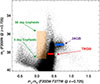 |
Fig. 1. Expected CMD of a z = 0.725 stellar population. The apparent magnitudes and colors are based on stars in a small portion of the LMC as observed by 2MASS in the J and H bands. The magnitudes have been corrected by distance while assuming the stars are at z = 0.725 (h = 0.74) but not magnified. Popular SCs are marked: the JAGB in blue, the TRGB in red, and Cepheids in the orange rectangle. The TRGB appears at mJ ≈ 38.25. There are N* ≈ 120 000 stars with mJ < 40. |
3. Probability of magnification
The magnification experienced by luminous stars in the Dragon is a combination of the macromodel magnification and magnification by microlenses in the A370 cluster’s ICM. For microlensing to take place, a microlens’ distortion in the magnification pattern must intersect the line of sight to a star in the Dragon. The probability that this will happen can be thought of as an optical depth, where “optically thick” means the probability is high. The transition to optically thick takes place when the effective surface mass density of microlenses is close to the critical surface mass density, Σeff ≡ μtΣ* ≈ Σcrit (Diego et al. 2018; Palencia et al. 2024a), where μt is the tangential component of the macromodel magnification defined as the product of radial and tangential magnifications, μm = μtμr, and Σ* is the microlens surface mass density. At the position of the Dragon, Σ∗ ≈ 30 M⊙ pc−2 (Li et al. 2024), and for the redshifts of A370 and the Dragon Σcrit = 3640 M⊙ pc−2 (Diego et al. 2024). This means the optically thick regime corresponds to μm ≳ 120. The macromodel magnification varies along the Dragon arc, weakly along the CC but with strong dependence on d, the separation from the CC. Typical values of the macromodel magnification, μm, range from a few tens when d is a few arcseconds to μm ≫ 100 when d is a fraction of an arcsecond. The exact location of the CC is unknown, and different models predict different locations, but in smooth macromodels, and near the CC, the magnification scales as μm = A/d, where A is a parameter that varies along the CC but typically takes values 30″ ≲ A ≲ 100″ (Diego et al. 2025, their Fig. 7).
Depending on the value of μm, which mostly depends on the separation d from the cluster CC, the probability distribution function (PDF) of magnification and the role of microlenses varies. At d > 2″, in the optically thin regime, μm < 100, and the PDF of the magnification has a relatively narrow peak near μm and a long tail scaling as μ−3 for magnifications ≫μm. Very close to the CC, when μm ≫ 100 in the optically thick regime, the microlenses play a very important role in shaping the magnification PDF. In this regime, microlenses introduce constant small-scale perturbations in the deflection field and increase its curvature. Because the magnification is inversely proportional to the curvature of the deflection field, the most likely value for the magnification drops below μm, and the PDF of the magnification becomes a lognormal. Between these two extremes, the PDF transitions between the two limiting shapes as shown in Figure 2. The curves in Figure 2 were obtained from inverse ray tracing of large simulations (Palencia et al. 2024a)1 with a pixel size equivalent to ≈300 R⊙, the size of a large star. Smaller stars can attain magnifications ≳10 000 when they cross a microcaustic, but that is not reproduced by the curves in Figure 2. Such enormous magnification factors can typically be maintained for only hours to a few days, depending on the star’s radius and its velocity relative to the microcaustic.
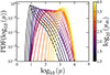 |
Fig. 2. Probability distribution of total magnification, P(μ), after accounting for macromodel and microlenses. Each curve is for a fixed macromagnification μm as indicated by the curve’s color and the color bar on the right. As explained in the text, μm mainly depends on separation from the cluster CC. The curves were derived with the code M_SMiLe (Palencia et al. 2024b), which computes the PDF of magnification for any combination of redshifts, μm, and Σ*. |
The PDFs of the magnification have an important property that decreases the uncertainty in the magnification. When Σeff ≫ Σcrit, the PDF becomes a well-determined lognormal similar to the rightmost curve (yellow) in Figure 2 regardless of the value of μm. The magnification at the CC (distorted by microlenses) reaches a maximal distribution (yellow curve in Figure 2) that we refer to as “the wall of magnification”, or simply “the wall” because no higher magnification is possible. The wall is expected to appear in all lens models and depends mostly on the value of Σ* (Palencia et al. 2024a). For a given Σ*, transient objects detected sufficiently close to the CC are affected by the same PDF (the wall), and the shape of the wall can be estimated from the value of Σ* obtained from the data via SED fitting of the intracluster light and the redshift of the lensed galaxy. The peak of the distribution is primarily determined by Σ*. Lower values of Σ* shift slightly the peak toward higher values, increasing the chance of seeing lensed stars near the CC. However, this often requires pushing the CC outwards (i.e., reducing Σ*) by increasing the redshift of the source. However this also increases the luminosity distance which makes the relatively small gain in magnification worthless (in terms of increasing the probability of detecting a lensed star). This enables robust forward modeling of the lensed stars (including features such as the sharp jump in the luminosity function due to the TRGB) through the known magnification PDF, to give a direct confrontation with observations.
4. The CMD of magnified bright stars
To simulate deep JWST observations of stars in an LMC-like galaxy at z = 0.725 crossing the cluster caustic of A370, we combined the stellar population shown in Figure 1 with the magnification PDF shown in Figure 2. We assigned each star a random macromodel magnification in the range 50 < μm < 5000 following the canonical PDF of macromodel magnification,  (Schneider et al. 1992). The lower limit μm = 50 corresponds to the lowest macromodel magnification expected in portions of the Dragon galaxy where individual stars can still be detected through microlensing, (e.g., Meena et al. 2023a). The upper limit μm = 5000 corresponds to the highest peak in the microlensed lognormal pdf shown in Figure 2 expected near the cluster CC. This peak is lower than the macromodel magnification near the CC owing to the effect of microlenses (Diego et al. 2018; Palencia et al. 2024a). Next, for each μm we computed P(μmicro) according to the value of μm. Each P(μmicro) resembles a curve in Figure 2. Finally, we randomly assigned μmicro from the generated P(μmicro) and computed the apparent magnitude after lensing amplification according to
 (1)
(1)
where MLMC is the observed AB magnitude in J or H (Ripoche et al. 2020), while 18.5 and 43.12 are the distance moduli to the LMC and z = 0.725, respectively (for h = 0.74), and −0.59 = −2.5log10(1 + z) is the bandwidth correction. This ignores the K correction by making the simplifying assumption that at z = 0.725, the rest J-band redshifts into F200W and that the filter responses are similar. The resulting apparent magnitudes are shown in Figure 3. For h = 0.68, all stars would be ≈0.18 fainter, but even in that case many NESCs from the three groups, Cepheids, JAGB, and TRGB should be above the detection limit (shown as a horizontal line in the figure for the case of deep JWST observations).
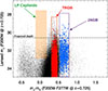 |
Fig. 3. Color–magnitude diagram of the stars in Figure 1 at z = 0.725 after being magnified by A370 and microlenses (Equation 1). The red points correspond to stars in the narrow TRGB magnitude range marked in red in Figure 1, and the blue dots correspond to stars in the blue JAGB region. The random magnifications spread the stars’ magnitudes over the ranges shown, but the magnification is wavelength-independent. A depth of 30.6 mag in F200W, shown by the horizontal dashed line, is needed to measure the TRGB knee feature. This detection limit is achievable with JWST in exposures of 16.7 hours, and there are ≈1100 stars brighter than this limit. |
As discussed in Sect. 3, the magnifications adopted in this calculation assume large stars with R* = 300 R⊙. Smaller stars, such as those in the TRGB with maximum radius R* ≈ 100 R⊙, can have maximum magnifications a factor (300/R*)0.5 larger (that is, 0.75 mag brighter for stars with R* = 75 R⊙) during a microcaustic crossing. This will promote a few more NESCs – ones very close to a microcaustic when observed – above the detection limit and slightly increase the numbers shown in Figure 3.
The calculation described above is nearly independent of the particular macrolens model because we are considering an arbitrary area containing a fixed number of stars and adopting the canonical PDF for the macromodel values (which most valid lens models should follow). In a realistic scenario, one should consider a particular lens model, or even better a range of models where discrepancies in the magnification at a given position of a factor ≈2 are expected near the critical curve (Meneghetti et al. 2020). Also, within a particular model, the strength of the CC (i.e., the parameter A in the magnification law μ = A/d) can vary along the critical curve, as recently shown for the particular case of the Dragon (Diego et al. 2025). Here we are not interested in predicting the exact number of NESC microlensing events in the Dragon but rather in showing how an LMC analog would appear at the redshift of the Dragon provided a macromodel caustic crosses the entire galaxy (as it does for the Dragon).
5. Lensed luminosity function
The transient events identified by Fudamoto et al. (2025) provided a first indication of the LF of the Dragon’s stars. Figure 4 compares the result to Sect. 4’s predictions. The drop in observed events at F200W ≈ 28 comes from the limiting magnitude of the observations. The two LFs were computed independently with normalization by the LMC’s stellar surface density. The agreement in normalization is an interesting coincidence, but the agreement in slope is consistent with the luminous LMC population being a good representation of the luminous Dragon population. Different values of h would move the predicted LF horizontally in the plot. For h = 0.68, stars at z = 0.725 would be 8.8% farther away (in luminosity distance) and 0.18 mag fainter. For a power-law LF, such a shift could not be distinguished from a different stellar surface density (a vertical shift), but in fact the LMC LF has a “knee” at the TRGB jump, below which the number of stars dramatically increases. The sharp TRGB jump (Figure 1) gets smoothed out by the probability of magnification (Figure 2), but the only TRGB stars that can be seen are those with the highest magnification close to the CC. That means the magnifications of the observed TRGB stars follow the magnification wall and form a “knee” in the LF as shown in the Figure 4 inset. The knee occurs at mJ ≈ 38.25 before magnification and mJ ≈ 30 as observed. The observed magnitude of this knee depends on the value of h as shown in the Figure 4 inset, with a change of ≈0.2 mag for the two values of h considered (vertical lines in the inset). The exact position of the knee is determined by the shape of the magnification wall, which depends mostly on the surface density Σ* of stars from the intracluster medium at the Dragon position. This dependence can be modeled (Palencia et al. 2024a) once Σ* is measured from photometry of the intracluster light. A change of 0.2 magnitudes in the position of the knee corresponds to a change in the peak of the magnification of the wall of ≈20%. As shown by Palencia et al. (2024a), at high effective surface mass density (Σeff > 50 × Σcrit) near the CC, the magnification wall approaches a lognormal peaking at magnification μp ≈ 0.35μm × (50Σcrit/Σeff) = 17.5μrΣcrit/Σ*, i.e., independent of μm but inversely proportional to Σ*. This scaling is derived from the top-right panel of Fig. 21 in Palencia et al. (2024a) in the regime Σeff/Σcrit ≫ 1 (power law with triangles, which is the dominant mode in this regime, as shown by the amplitude in the top-left panel). This type of scaling is an approximation (yet a good one), since this extreme regime has not been properly explored with high resolution and very large simulations. From Fig. 21 in Palencia et al. (2024a) we see that for Σeff/Σcrit ≫ 1 the PDF becomes a lognormal with approximately constant amplitude and width (σ), but peaking at a position inversely proportional to Σeff = μtΣ*. Hence, as we approach the CC (increase μt with μr ≈ cte), the dependency on μt cancels out, leaving only a dependence on Σ*, which determines the peak position of the magnification wall (yellow curve in Fig. 2). The radial magnification μr varies slowly near CCs and is typically close to 1. Therefore the dependence of the knee’s apparent magnitude on the macromodel is weak. A different macromodel may increase or reduce the region (area around the CC) of validity of the PDF describing the wall of magnification. This will impact the number of detections of TRGB stars (or amplitude of the LF in Figure 4) but not the apparent magnitude of the knee, which is mostly determined by the values of Σ* and H0. The above expression use μm = μtμr, where μt and μr are the tangential and radial components of the magnification respectively, and Σeff = μtΣ* Palencia et al. (2024a). For the Dragon, Σcrit = 3640 M⊙ pc−2, μt ≈ 1.5, and Σ∗ ≈ 30 M⊙ pc−2, and the magnification wall should peak at log10(μp)≈3.5, in good agreement with the yellow curve in Fig. 2. Measuring Σ* to the 20% precision needed to distinguish between h = 0.68 and h = 0.74 represents a challenge, but that can be mitigated by modeling the spatial distribution of microlensing events around the CC, which also depends on Σ*. A higher value of Σ* increases the probability of magnification far from the cluster CC and increases the detection rate in those distant regions. Conversely, a larger value of Σ* decreases the magnification where the PDF of the wall of magnification peaks, thus increasing the apparent magnitude of the knee feature and requiring deeper observations to observe the knee. If measuring Σ* to the precision needed to use the knee feature as a distance indicator proves too difficult, the equation can be turned around, and the knee feature can be used to measure Σ* for a given h. This is of special interest for constraining the microlensing, including the number of primordial black holes, a popular dark matter (DM) candidate.
In summary, deep observations will detect a large number of TRGB stars in the Dragon, thus measuring the LF down to AB ≈30.6. The sharp TRGB knee feature should be observed at F200W ≈ 30 mag as shown in the inset of Fig. 4. After modeling the PDF of the magnification wall with the value of Σ*, also measured from the deep observations, one can forward model the knee feature and distinguish between the two values of h by measuring the magnitude of the knee in the LF. Alternatively, one can use the knee feature’s magnitude together with h known from other observations to constrain the number of microlenses (Σ*), including DM candidates. In combination with photometric measurements of the intracluster light, it may even be possible to constrain the mass function of microlenses and distinguish between IMF models, such as Salpeter or Chabrier because the latter has a much smaller contribution to Σ* from low-mass stars, which are expected to be well represented in the older population of the intracluster medium.
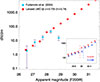 |
Fig. 4. Luminosity function (LF) of observed transients in the Dragon galaxy (Fudamoto et al. 2025) compared with the expected LF (red dots). Error bars on the blue points are from Poisson statistics, and the drop in observed events at F200W ≈ 28 is from the limiting magnitude of the observations. The red points correspond to a randomly selected subsample of 180 000 luminous stars from the LMC. The expected LF is that of an LMC-like galaxy at z = 0.725 in a cosmology with h = 0.74 (Figure 3). The inset shows a zoomed-in portion of the lensed LF around the knee of the lensed TRGB with dark blue dots showing the LF for h = 0.68. The two vertical dashed lines mark the position of the knee for each cosmology. |
6. Discussion
6.1. Dark matter and the spatial distribution of transients
An interesting point to consider is the spatial distribution of detected stars. Naturally the faintest stars require the largest magnification factors to be detected, while intrinsically brighter stars can be detected at more modest magnifications. The total magnification correlates with the macromodel magnification, so we expect the faintest stars to concentrate around the cluster CC as illustrated in Figure 5. The TRGB stars will be detected only near the cluster CC, whereas stars in the JAGB region are intrinsically brighter and can be detected farther from the CC. The most luminous Cepheid stars will hardly concentrate near the CC at all. Overall, the highest density of transients will be found at the CC, as expected for a relatively steep LF (Diego et al. 2024). Given the similarity of the LMC LF to the observed one (Figure 4), stars detected in observations of the Dragon reaching magnitude 30.6 should trace the cluster CC with precision similar to that shown in Figure 5. More importantly, the faintest detections will also trace the smaller CCs of DM substructures away from the main cluster CC. This will effectively map DM to very small scales (Diego et al. 2024).
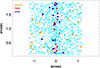 |
Fig. 5. Simulated spatial distribution of lensed events. The dashed vertical line represents the cluster CC. The points represent all 1122 stars above 30.6 mag in Figures 3 and 4. Red and dark blue dots represent detected stars in the TRGB and JAGB regions respectively. Orange dots represent the most luminous stars in the LMC (MJ < 34 before lensing and MJ < 30.6 after lensing). Cyan points represent other stars, mostly highly microlensed red giants intrinsically fainter than the TRGB. The x location of each star was derived from a simple model where μm scales with d as μm = 60″/d. This gives μm = 50 at the maximum d illustrated. The y coordinate shown is a random value between |


A complication for mapping DM substructures is that clusters of luminous stars in the Dragon may also produce a cluster of microlensing events. These could be mistakenly interpreted as the effect of a DM substructure, but the two scenarios can be distinguished by using the other counterimages of the arc. In the DM substructure scenario, each counterimage’s microlensing is affected by its own DM, and there will be no correlation in the locations of high densities of transients. In the clustering of Dragon stars scenario, individual transients will not correlate, but concentrations of transients should be seen at the same locations in all counterimages of the same star cluster because the star clusters offer a localized high density of sources to be lensed. Finally, as mentioned earlier, the magnification of the peak of the wall, and hence the position of the knee feature from the TRGB stars, anticorrelates with Σ*, opening another avenue to constrain models of DM, such as primordial black holes, by studying the distribution of events in luminosity.
6.2. Lensed Cepheids and magnification
The most luminous variable stars in the Dragon can appear as transients even without microlensing, i.e., even if they are far from the CC where Σeff < Σcrit. Such luminous stars include the rare Cepheids with P > 50 days. Detecting these Cepheids in the Dragon offers a potentially new avenue to constrain H0 in a redshift range never tested before with this type of standard candle. However, the macromodel magnification, μm, can be uncertain by ∼50% near the CC (Meneghetti et al. 2020), creating a challenging degeneracy between the distance modulus and the magnification. In addition, microlenses will alter the Cepheid light curves. We discuss microlensing in more detail in Section 6.4.
The degeneracy between distance modulus and magnification can be turned around, and Cepheids can be used to constrain the magnification at their positions, which in turn improves the precision of the lens model and thus the forward modeling of the TRGB or JAGB. This may prove to be the most practical use for Cepheids.
6.3. Cepheid detection limit
If JWST can detect Cepheids in the Dragon, a natural question is how much farther away can JWST detect them. The Spock arc, a z = 1.0054 galaxy that is highly magnified by the galaxy cluster MACS0416, offers a case in point. Spock’s luminosity distance is ≈50% larger than the Dragon’s, and the increase in distance modulus minus bandwidth correction is ≈0.7 mag. To focus on the small region of the Spock galaxy that is strongly magnified, we adopted the brightest Cepheids in the central region of the LMC, specifically the Riess et al. (2019) sample containing 70 luminous Cepheids. From the I and H measurements (Riess et al. 2019), we estimated rest J-band magnitudes by a simple average and transformed them to AB. These stars were then placed at z = 1.0054 and magnified by the same probabilities as in Figure 2. The sample was simulated ten times with sufficient separation in time (years) to make the magnitudes uncorrelated. The resulting apparent magnitudes are shown in Figure 6. From this figure, highly magnified long-period Cepheids in Spock would be accessible with approximately 2 hour JWST exposures reaching F200W ≈ 29.5 or even deeper with F150W2. Magnifications larger than the few thousand shown in this figure are still possible, so in principle Cepheids could be observed in Spock during a microlensing event with even shorter exposures. These events are often short-lived, with large magnification factors lasting a few weeks, but in some scenarios, large magnification factors can be maintained during several years. For example, a DM substructure or one of the many thousands of globular clusters in the ICM can produce long-term high magnifications relatively far from the CC. This type of rare scenario is suspected to be responsible for the long-lasting high magnification of stars such as Godzilla (Diego et al. 2022) and Mothra (Diego et al. 2023b). The high magnification factors in these two cases (μ > 2000) would make a bright Cepheid detectable for several years, potentially allowing measurement of its period.
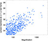 |
Fig. 6. Lensed Cepheids in the Spock arc at z = 1.0054. The plot shows ten magnification realizations of the 70 luminous Cepheid stars in the LMC (Riess et al. 2019) but placed at the redshift of the Spock arc and magnified by the galaxy cluster plus microlenses. The J-band redshifts to 2.5 μm, i.e., between JWST’s F200W and F277W bands. One Cepheid from this sample is expected to be observed in observations reaching depth F200W ∼ 29.5 AB amg. |
Although very challenging, the possibility of detecting Cepheids up to z = 1 is exciting. Several transients in the Spock arc have been identified first with HST (Rodney et al. 2018; Kelly et al. 2022) and more recently with JWST (Yan et al. 2023). Additional transients have been found behind the same cluster in a different (and much larger) spiral galaxy, Warhol at z = 0.9396 (Chen et al. 2019; Kaurov et al. 2019; Yan et al. 2023), where the Cepheids would be ≈0.2 mag brighter than in Figure 6. Some of the observed transients may have been due to Cepheid variability, and long-term monitoring of these arcs could determine that. Cepheids should reappear at regular times, although microlensing distortions to the magnification will contaminate the light curves.
6.4. Cepheids in the Dragon and the role of microlenses
The above discussion about Cepheids has included the role of microlenses only at a statistical level, that is, accounting only for the broadening of the probability of magnification (Figure 2). However, microlensing perturbs the stars’ light curves and thus complicates the determination of the periods and even the recognition of periodicity. To explore the effect of microlenses, we simulated the light curve of a long-period Cepheid near the critical curve in the Dragon arc. We chose the Dragon instead of Spock or Warhol because of its lower redshift (z = 0.725) and larger intersection of the background galaxy with the cluster caustic. Both factors are expected to greatly increase the rate of microlensing events, as demonstrated already with the detection of more than 40 events (Fudamoto et al. 2025).
The specific model is a P = 50 days Cepheid in a region where μm = 100 × 1.61 = 161 and on the side of the critical curve with negative parity. From Appendix A in Diego et al. (2024), we estimate 0.58 kpc2 in the Dragon (in the source plane) have macromodel magnification above this value. This represents ≈3% the area of the LMC. Extrapolating the number of detectable luminous Cepheids (13) in Persson et al. (2004), there is ≈40% chance we would have one of these Cepheids in the region with macromodel magnification μ > 161. During microlensing events, magnification is stronger in images with negative parity, thus maximizing the possibility of their detection. Cepheids with P ≥ 50 days are rare but more likely to be observed because they require less magnification. The Cepheid’s absolute J magnitude (Vega system) comes from Storm et al. (2011): MJ = −3.18[log10(P/days)−1]−5.22. We simulate the periodic variation of the Cepheid as a simple sinusoid with amplitude 0.5 mag between maximum and minimum. This is a typical variation for many classic Cepheids (e.g., Ulaczyk et al. 2012). The sinusoidal shape (fundamental mode) is also a reasonable approximation although many Cepheids exhibit more complicated patterns. At the redshift of the Dragon, J redshifts to ∼2.2 μm (near JWST F200W). We transform Vega to AB magnitudes following Maíz Apellániz (2007), and applied the bandwidth correction 2.5log10(1 + z) and the distance modulus, 43.12 (for z = 0.7251 and H0 = 74 km s−1 Mpc−1). For the microlenses, we assume a surface mass density Σ* = 30 M⊙/pc2, consistent with the estimate of Li et al. (2024). The combination of Σ* and μm gives an effective surface mass density Σeff = 6440 M⊙/pc2 = 1.77 × Σcrit. The range Σcrit < Σeff < 2 × Σcrit is where we expect microlensing events to be most common (Diego et al. 2018; Palencia et al. 2024a). We assume a relative velocity vrel = 1000 km s−1 between the Cepheid and the web of microcaustics, a typical velocity for the redshifts of A370 and the Dragon (Windhorst et al. 2018). For this illustration, we choose a trajectory at an angle of 45° from the macromodel deflection field. For the chosen relative velocity, the Cepheid crosses one microcaustic approximately every year and the whole simulated source plane in ≈50 years. (The crossing time would be ≈30 years for a trajectory at 90°). The simulation’s resolution is 2 nanoarcsec/pixel, and the light curves are sampled at ≈3 day intervals.
The sinusoidal light curve (in apparent magnitudes) is corrected for macro+microlensing magnification by subtracting the term 2.5log10(μmicro), where μmicro is the net magnification from the macromodel plus microlensing. Figure 7 shows a ≈11 year portion of the resulting light curve. The effect of the underlying magnification from the macromodel plus micromodel is shown as a blue curve, while the net effect including the sinusoidal periodic variation of the Cepheid is shown as a black curve. The simulation shows that most of the time, the Cepheid is too faint to observe. Observations reaching F200W = 30.6 mag could follow the Cepheid for about a year (7−8 in Figure 7), detect its periodicity, and measure a period. In the Figure 7) example, the 50-day period Cepheid is detectable ≈14% of the time. However, this fraction depends on the macromodel μ and the microlensing Σ*. Closer to the CC, or for the same macromodel magnification μ but with a higher value of Σ*, the fraction of time a Cepheid can be detected increases. Conversely, farther away from the CC and with smaller values of Σ* the fraction of time the same Cepheid is brighter than 30.6 mag in F200W decreases. Also, the situation presented in Figure 7 represents an optimistic scenario since it focuses around a region with a local overdensity of microcaustics. Exploring a larger area in the source plane with 5x longer light curves we find this ratio decreases to ≈8% (fraction of time the Cepheid is brighter than 30.6 mag in JWST’s F200W). Reducing the depth of the observations reduces also the fraction of time a Cepheid can be detected. For instance for 30 mag in F200W we find the Cepheid is observed ≈3% of the time, while for shallower observations (29 mag in F200W) observing a Cepheid at this redshift becomes very challenging with only ≈0.4% being detectable. Conversely, at fainter magnitudes we expect a higher ratio of success. For instance, with exposure times of 7.8 hours in the ultrawide filter F150W2, a 6000 K Cepheid star with apparent magnitude 31 is detected at 5σ in this filter. This would increase the fraction of time above this magnitude back to our optimistic ≈14% discussed earlier.
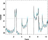 |
Fig. 7. Portion of the light curve of a P = 50 day Cepheid in the Dragon at macromodel magnification μm = 161 and under the influence of microlenses (Σ* = 30 M⊙/pc2). The effect of the underlying magnification from the macromodel plus micromodel is shown as a blue curve, while the net effect including the sinusoidal periodic variation of the Cepheid is shown as a black curve. The dotted line marks the detection limit of 30.6 mag in JWST’s F200W. |
Because the duration of a microcaustic crossing is much shorter than the Cepheid’s period, if the observations are carried only at depths F200W ∼ 29 mag, this will not provide sufficient data to recognize the star as a Cepheid. Deeper observations reaching F200W ≈ 30.6 mag are needed in order to see the periodic oscillations and measure the period. In the example shown in the figure, the ≈0.5 year period in year 2 offers the best chance to detect the Cepheid and measure its period. Approximately three full cycles of the Cepheid are contained between the peaks of the microlensing event. One would need ∼10 deep and regularly spaced observations in order to measure the period with enough precision, with more observations resulting in better precision. The same Cepheid can be observed again in future microlensing events which should help improve the measurement of its period.
In summary, microlenses boost the overall magnification and allow Cepheids to be detected, but the resulting fluctuations in the magnification make it more difficult to recognize the Cepheid’s periodic nature. The microlensing event at 7−8 years is a good example. Perhaps more damaging is that the magnification during a microlensing valley (that is, between the two peaks that bracket each microlensing event) can vary significantly from microlens to microlens. Also, for a given microlens, the valley magnification varies with the (unknown) distance to the cusp of the microcaustic. This introduces a stochastic element into the magnification which impedes the use of Cepheids as a standard candle. Despite that, Cepheids could be used to constrain the microlens magnification and thus the microlens’ mass.
7. Conclusions
We have simulated how the brightest stars in the LMC would appear if they are placed in the Dragon galaxy at redshift z = 0.725 and amplified by the galaxy cluster A370 and microlenses in the cluster’s ICM. The large magnification factors near the cluster CC combined with microlensing amplify the flux enough to make ≳1100 stars detectable in observations reaching 30.6 mag in F200W. This depth is within JWST’s reach and should be within the reach of future adaptive-optics-equipped extremely large telescopes on the ground. Dragon stars would be detected as transients (microlensing events) in difference images taken ≈1 year apart, an interval sufficient for the microlensing magnification to change. The large number of stars will allow accurate tracing of the cluster’s CC. More importantly, the faintest stars, such as the RGBs, will concentrate around the position of invisible DM substructures, which create their own small CC. This will allow mapping of the DM distribution down to scales of 104 M⊙.
Even accounting for the random effects of lensing, the observed LF of Dragon stars is expected to change slope at ≈30 mag. This knee feature is due to the large number of RGB stars that start to be detected at this magnitude, and the observed magnitude of the slope change will differ by 0.18 mag for H0 = 68 versus 74. Galaxies at lower redshifts would show the slope change at brighter magnitudes, for instance 0.4 mag brighter at z = 0.6. The observed magnitude of the knee feature is nearly independent of the lensing macromodel because the magnification PDF forms a universal lognormal shape–the wall of magnification–that depends mostly on Σ*. In order to differentiate between the two values of H0 (68 and 74 km s−1 Mpc−1), Σ* needs to be measured with better than 20% precision from photometric data, which might represent a challenge. Conversely, one could assume a fiducial value for H0 and use the observed magnitude of the knee to infer the value of Σ*, exploiting this as a novel method to constrain the abundance of compact DM.
Cepheids should also be detectable in the Dragon in observations reaching ≈30 mag and to z ≈ 1 in observations 0.7 mag deeper. Regular observations of the Dragon (or similar strongly lensed arcs) will allow construction of Cepheid light curves, although the derivation of their periods will be a challenging task because of the magnitude perturbations introduced by microlenses.
Galaxies such as Warhol and Spock at z ≈ 1 already show a wealth of transients. Most of these are likely red or blue supergiant stars undergoing microlensing, but some of them could be the first Cepheids at this redshift.
Acknowledgments
J.M.D. acknowledges support from projects PID2022-138896NB-C51 (MCIU/AEI/MINECO/FEDER, UE) Ministerio de Ciencia, Investigación y Universidades and SA101P24 (Junta de Castilla y Leon). RAW acknowledges support from NASA JWST Interdisciplinary Scientist grants NAG5-12460, NNX14AN10G and 80NSSC18K0200 from GSFC. We thank the anonymous referee for a constructive and insightful feedback.
References
- Anand, G. S., Riess, A. G., Yuan, W., et al. 2024, ApJ, 966, 89 [NASA ADS] [CrossRef] [Google Scholar]
- Chen, W., Kelly, P. L., Diego, J. M., et al. 2019, ApJ, 881, 8 [NASA ADS] [CrossRef] [Google Scholar]
- Cioni, M. R. L., Girardi, L., Marigo, P., & Habing, H. J. 2006, A&A, 448, 77 [NASA ADS] [CrossRef] [EDP Sciences] [Google Scholar]
- Diego, J. M., Kaiser, N., Broadhurst, T., et al. 2018, ApJ, 857, 25 [NASA ADS] [CrossRef] [Google Scholar]
- Diego, J. M., Pascale, M., Kavanagh, B. J., et al. 2022, A&A, 665, A134 [NASA ADS] [CrossRef] [EDP Sciences] [Google Scholar]
- Diego, J. M., Meena, A. K., Adams, N. J., et al. 2023a, A&A, 672, A3 [NASA ADS] [CrossRef] [EDP Sciences] [Google Scholar]
- Diego, J. M., Sun, B., Yan, H., et al. 2023b, A&A, 679, A31 [NASA ADS] [CrossRef] [EDP Sciences] [Google Scholar]
- Diego, J. M., Li, S. K., Amruth, A., et al. 2024, A&A, 689, A167 [NASA ADS] [CrossRef] [EDP Sciences] [Google Scholar]
- Diego, J. M., Sun, F., Palencia, J. M., et al. 2025, A&A, 703, A207 [NASA ADS] [CrossRef] [EDP Sciences] [Google Scholar]
- Freedman, W. L., Madore, B. F., Hatt, D., et al. 2019, ApJ, 882, 34 [Google Scholar]
- Freedman, W. L., Madore, B. F., Hoyt, T. J., et al. 2025, ApJ, 985, 203 [Google Scholar]
- Fudamoto, Y., Sun, F., Diego, J. M., et al. 2025, Nat. Astron., 9, 428 [Google Scholar]
- Furtak, L. J., Meena, A. K., Zackrisson, E., et al. 2024, MNRAS, 527, L7 [NASA ADS] [Google Scholar]
- Kaurov, A. A., Dai, L., Venumadhav, T., Miralda-Escudé, J., & Frye, B. 2019, ApJ, 880, 58 [NASA ADS] [CrossRef] [Google Scholar]
- Kelly, P. L., Diego, J. M., Rodney, S., et al. 2018, Nat. Astron., 2, 334 [NASA ADS] [CrossRef] [Google Scholar]
- Kelly, P. L., Chen, W., Alfred, A., et al. 2022, ArXiv e-prints [arXiv:2211.02670] [Google Scholar]
- Lee, M. G., Freedman, W. L., & Madore, B. F. 1993, ApJ, 417, 553 [Google Scholar]
- Li, S. K., Kelly, P. L., Diego, J. M., et al. 2024, ArXiv e-prints [arXiv:2404.08571] [Google Scholar]
- Madore, B. F., & Freedman, W. L. 1995, AJ, 109, 1645 [NASA ADS] [CrossRef] [Google Scholar]
- Madore, B. F., & Freedman, W. L. 2020, ApJ, 899, 66 [NASA ADS] [CrossRef] [Google Scholar]
- Mager, V. A., Madore, B. F., & Freedman, W. L. 2008, ApJ, 689, 721 [Google Scholar]
- Maíz Apellániz, J. 2007, ASP Conf. Ser., 364, 227 [Google Scholar]
- Meena, A. K., Chen, W., Zitrin, A., et al. 2023a, MNRAS, 521, 5224 [NASA ADS] [CrossRef] [Google Scholar]
- Meena, A. K., Zitrin, A., Jiménez-Teja, Y., et al. 2023b, ApJ, 944, L6 [NASA ADS] [CrossRef] [Google Scholar]
- Meneghetti, M., Davoli, G., Bergamini, P., et al. 2020, Science, 369, 1347 [Google Scholar]
- Newman, M. J. B., McQuinn, K. B. W., Skillman, E. D., et al. 2024, ApJ, 975, 195 [Google Scholar]
- Palencia, J. M., Diego, J. M., Kavanagh, B. J., & Martínez-Arrizabalaga, J. 2024a, A&A, 687, A81 [Google Scholar]
- Palencia, J. M., Diego, J. M., Kavanagh, B. J., & Martínez-Arrizabalaga, J. 2024b, Astrophysics Source Code Library [record ascl:2408.011] [Google Scholar]
- Persson, S. E., Madore, B. F., Krzemiński, W., et al. 2004, AJ, 128, 2239 [NASA ADS] [CrossRef] [Google Scholar]
- Planck Collaboration VI. 2020, A&A, 641, A6 [NASA ADS] [CrossRef] [EDP Sciences] [Google Scholar]
- Riess, A. G., Casertano, S., Yuan, W., Macri, L. M., & Scolnic, D. 2019, ApJ, 876, 85 [Google Scholar]
- Ripoche, P., Heyl, J., Parada, J., & Richer, H. 2020, MNRAS, 495, 2858 [NASA ADS] [CrossRef] [Google Scholar]
- Rodney, S. A., Balestra, I., Bradac, M., et al. 2018, Nat. Astron., 2, 324 [Google Scholar]
- Schneider, P., Ehlers, J., & Falco, E. E. 1992, Gravitational Lenses, XIV (New York: Springer-Verlag) [Google Scholar]
- Storm, J., Gieren, W., Fouqué, P., et al. 2011, A&A, 534, A94 [CrossRef] [EDP Sciences] [Google Scholar]
- Udalski, A., Soszynski, I., Szymanski, M., et al. 1999, Acta Astron., 49, 223 [Google Scholar]
- Ulaczyk, K., Szymański, M. K., Udalski, A., et al. 2012, Acta Astron., 62, 247 [NASA ADS] [Google Scholar]
- Weinberg, M. D., & Nikolaev, S. 2001, ApJ, 548, 712 [Google Scholar]
- Welch, B., Coe, D., Diego, J. M., et al. 2022, Nature, 603, 815 [NASA ADS] [CrossRef] [Google Scholar]
- Windhorst, R. A., Timmes, F. X., Wyithe, J. S. B., et al. 2018, ApJS, 234, 41 [NASA ADS] [CrossRef] [Google Scholar]
- Yan, H., Ma, Z., Sun, B., et al. 2023, ApJS, 269, 43 [NASA ADS] [CrossRef] [Google Scholar]
The M_SMiLe (Palencia et al. 2024a) code is at https://github.com/ChemaPalencia/M_SMiLe
All Figures
|
Fig. 1. Expected CMD of a z = 0.725 stellar population. The apparent magnitudes and colors are based on stars in a small portion of the LMC as observed by 2MASS in the J and H bands. The magnitudes have been corrected by distance while assuming the stars are at z = 0.725 (h = 0.74) but not magnified. Popular SCs are marked: the JAGB in blue, the TRGB in red, and Cepheids in the orange rectangle. The TRGB appears at mJ ≈ 38.25. There are N* ≈ 120 000 stars with mJ < 40. |
| In the text | |
|
Fig. 2. Probability distribution of total magnification, P(μ), after accounting for macromodel and microlenses. Each curve is for a fixed macromagnification μm as indicated by the curve’s color and the color bar on the right. As explained in the text, μm mainly depends on separation from the cluster CC. The curves were derived with the code M_SMiLe (Palencia et al. 2024b), which computes the PDF of magnification for any combination of redshifts, μm, and Σ*. |
| In the text | |
|
Fig. 3. Color–magnitude diagram of the stars in Figure 1 at z = 0.725 after being magnified by A370 and microlenses (Equation 1). The red points correspond to stars in the narrow TRGB magnitude range marked in red in Figure 1, and the blue dots correspond to stars in the blue JAGB region. The random magnifications spread the stars’ magnitudes over the ranges shown, but the magnification is wavelength-independent. A depth of 30.6 mag in F200W, shown by the horizontal dashed line, is needed to measure the TRGB knee feature. This detection limit is achievable with JWST in exposures of 16.7 hours, and there are ≈1100 stars brighter than this limit. |
| In the text | |
|
Fig. 4. Luminosity function (LF) of observed transients in the Dragon galaxy (Fudamoto et al. 2025) compared with the expected LF (red dots). Error bars on the blue points are from Poisson statistics, and the drop in observed events at F200W ≈ 28 is from the limiting magnitude of the observations. The red points correspond to a randomly selected subsample of 180 000 luminous stars from the LMC. The expected LF is that of an LMC-like galaxy at z = 0.725 in a cosmology with h = 0.74 (Figure 3). The inset shows a zoomed-in portion of the lensed LF around the knee of the lensed TRGB with dark blue dots showing the LF for h = 0.68. The two vertical dashed lines mark the position of the knee for each cosmology. |
| In the text | |
|
Fig. 5. Simulated spatial distribution of lensed events. The dashed vertical line represents the cluster CC. The points represent all 1122 stars above 30.6 mag in Figures 3 and 4. Red and dark blue dots represent detected stars in the TRGB and JAGB regions respectively. Orange dots represent the most luminous stars in the LMC (MJ < 34 before lensing and MJ < 30.6 after lensing). Cyan points represent other stars, mostly highly microlensed red giants intrinsically fainter than the TRGB. The x location of each star was derived from a simple model where μm scales with d as μm = 60″/d. This gives μm = 50 at the maximum d illustrated. The y coordinate shown is a random value between |
| In the text | |
|
Fig. 6. Lensed Cepheids in the Spock arc at z = 1.0054. The plot shows ten magnification realizations of the 70 luminous Cepheid stars in the LMC (Riess et al. 2019) but placed at the redshift of the Spock arc and magnified by the galaxy cluster plus microlenses. The J-band redshifts to 2.5 μm, i.e., between JWST’s F200W and F277W bands. One Cepheid from this sample is expected to be observed in observations reaching depth F200W ∼ 29.5 AB amg. |
| In the text | |
|
Fig. 7. Portion of the light curve of a P = 50 day Cepheid in the Dragon at macromodel magnification μm = 161 and under the influence of microlenses (Σ* = 30 M⊙/pc2). The effect of the underlying magnification from the macromodel plus micromodel is shown as a blue curve, while the net effect including the sinusoidal periodic variation of the Cepheid is shown as a black curve. The dotted line marks the detection limit of 30.6 mag in JWST’s F200W. |
| In the text | |
Current usage metrics show cumulative count of Article Views (full-text article views including HTML views, PDF and ePub downloads, according to the available data) and Abstracts Views on Vision4Press platform.
Data correspond to usage on the plateform after 2015. The current usage metrics is available 48-96 hours after online publication and is updated daily on week days.
Initial download of the metrics may take a while.