| Issue |
A&A
Volume 706, February 2026
|
|
|---|---|---|
| Article Number | A155 | |
| Number of page(s) | 14 | |
| Section | The Sun and the Heliosphere | |
| DOI | https://doi.org/10.1051/0004-6361/202554166 | |
| Published online | 06 February 2026 | |
First ionization potential bias evolution in an emerging active region as observed in SPICE synoptic observations
1
Southwest Research Institute Boulder CO 80302, USA
2
Smead Aerospace Engineering Sciences Department, University of Colorado Boulder Boulder CO, USA
3
University College London, Mullard Space Science Laboratory Holmbury St. Mary Dorking Surrey RH5 6NT, UK
4
Space Science Division, Naval Research Laboratory Code 7684 Washington DC 20375, USA
5
ETH-Zurich, Hönggerberg Campus HIT Building Zürich, Switzerland
6
PMOD/WRC Dorfstrasse 33 7260 Davos Dorf, Switzerland
★ Corresponding author: This email address is being protected from spambots. You need JavaScript enabled to view it.
Received:
17
February
2025
Accepted:
3
December
2025
Abstract
Aims. We investigate the time evolution of relative elemental abundances in the context of the first ionization potential effect focusing on an active region (AR). Our aim is to characterize this evolution in different types of AR structures as well as in different atmospheric layers. We wish to assess how the measured changes relate to different magnetic topologies by computing abundance enhancement in different conditions using the ponderomotive force model.
Methods. Leveraging SPICE (Spectral Imaging of the Coronal Environment) spectroscopic observations of extreme ultraviolet lines from ions formed across a broad temperature range – from the upper chromosphere to the low corona –, we performed relative abundance ratios following differential emission measure analysis. This methodology yields abundance maps from low, intermediate, and high first ionization potential elements.
Results. We obtained the temporal evolution of a number of abundance ratios for different structures on the Sun. We compared these results with the outcomes of the ponderomotive force model. We find good correlation between the model and our results, suggesting an Alfvén-wave driven fractionation of the plasma. Fan loops, loop footpoints and AR boundaries exhibit coronal abundances, while the AR core shows more photospheric-like composition. A slow and steady increase in the Mg/Ne first ionization potential bias values is observed, starting around 1.5 and increasing by about 50% after two days. The S/O evolution coupled with the model provides evidence of resonant waves fractionating the plasma in transition region structures.
Key words: Sun: abundances / Sun: corona / Sun: transition region / Sun: UV radiation
© The Authors 2026
 Open Access article, published by EDP Sciences, under the terms of the Creative Commons Attribution License (https://creativecommons.org/licenses/by/4.0), which permits unrestricted use, distribution, and reproduction in any medium, provided the original work is properly cited.
This article is published in open access under the Subscribe to Open model. This email address is being protected from spambots. You need JavaScript enabled to view it. to support open access publication.
1. Introduction
The growing number of solar science missions in the last two decades has enabled solar physicists to address a great number of unresolved questions regarding plasma dynamics and mechanisms in the solar atmosphere. Solar Orbiter (SolO), the joint ESA and NASA solar and heliospheric mission, was launched in February 2020 (Müller et al. 2020).
Using the onboard SPICE (Spectral Imaging of the Coronal Environment) instrument, we focus on the first ionization potential (FIP) as one of the discriminating factors when it comes to elemental abundance variations. One way to characterize these compositional variations is through the “FIP effect” (Meyer 1985, 1991), whereby elements with a low FIP are enhanced in abundance within certain coronal structures relative to high-FIP elements.
This “FIP effect” is characterized as the ratio between an element’s coronal and photospheric abundances (for element X, noted AbXcoronal and AbXphotospheric):
 (1)
(1)
Because it is challenging to determine the absolute abundance of elements relative to hydrogen in the upper solar atmosphere, we instead rely on relative abundances. We compare the ratios of radiances between spectral lines of different elements to study their composition. Several studies have investigated the dependency of this ratio, the “FIP bias”, on the type of solar region, magnetic flux, and solar cycle, and increasing interest has focused on its temporal evolution (see Section 1.2). However, few studies have examined how the FIP bias evolves over time specifically within the transition region or across multiple atmospheric layers – a focus that distinguishes the present work (Widing & Feldman 2001; Baker et al. 2015). Sheeley (1995), Widing (1997), Young & Mason (1997), and Widing & Feldman (2001) found photospheric plasma composition in newly emerged loops, indicating that flux emergence provides a potential reservoir of low-FIP bias plasma to mix with high-FIP bias plasma contained within active region (AR) coronal loops. Understanding the mechanisms by which this material enters AR coronal loops and the timescales over which plasma mixing occurs, and therefore the evolution of the FIP bias, is crucial to investigating the link between the underlying magnetic field and the coronal plasma (Baker et al. 2015).
Earlier investigations of the FIP effect have mainly focused on the corona (Baker et al. 2018; Mihailescu et al. 2022; Baker et al. 2022; Mihailescu et al. 2023). In contrast, studies treating the Sun as an unresolved source found little to no evidence of FIP fractionation at transition region temperatures (Laming et al. 1995), and spatially resolved measurements at those temperatures revealed FIP-related signatures only in select structures (Sheeley 1995; Widing & Feldman 2001). With Solar Orbiter’s improved spatial resolution and its closer approach to the Sun, exploring FIP fractionation in the transition region is now particularly compelling.
As mentioned in Baker et al. (2015) and references therein, current thinking suggests that emerging closed loops begin with a photospheric composition, which then transitions to a coronal one in the following days. However, the timescales and exact mechanisms for this transformation are not fully understood. Widing & Feldman (2001) used the Skylab spectroheliograph to investigate the Mg VI/Ne VI ratio. Their work concluded that the FIP bias increased shortly after AR emergence (Δt < 1 day) to reach coronal values after a few days (Δt > 2/3 days), and a correlation between the sunspot growth and increasing in FIP bias has also been established. It is thought that emerging loops of photospheric composition reconnect with older structures (i.e., preexisting loops, formed before the flux emergence and exhibiting higher FIP bias) and lead to fractionated plasma being brought up to the corona, most likely through interchange reconnection. The timescale and mechanisms of this mixing is thought to be on the order of days (Baker et al. 2015; Widing & Feldman 2001).
The aim of this project is to investigate the variability of FIP bias during the emergence phase of an AR, leveraging the unique opportunity provided by the SPROUTS (Synoptic PRogram of Out of RemoTe Sensing observations) to continuously monitor the Sun. We focus on the FIP bias evolution over time, across different structural features, and through various layers of the solar atmosphere specifically within the temperature range of  –6.0. These changes in elemental abundances are then compared with predictions made by the ponderomotive force model.
The ponderomotive force (see Laming 2015; Laming et al. 2019) is the most widely accepted explanation for the FIP effect and the inverse FIP effect (an enhancement in the abundance of high FIP elements). It posits that Alfvén waves generated either in the corona or arising from the photosphere travel to chromospheric heights where they encounter strong density gradients and thus are refracted and reflected. That change in direction leads to the “ponderomotive force”. This force separates the ions from the neutrals – the ions traveling toward areas of high wave electric energy density, leading to the observed FIP effect. The newly fractionated plasma is then brought upward by thermal and diffusion processes. For closed loops, the best match with observations comes with waves that are resonant. Alfvén waves propagate along magnetic field lines and can undergo resonance in the chromosphere, where their frequencies match natural oscillation modes of magnetic flux tubes. At resonance, the wave energy is efficiently converted into localized ponderomotive forces acting on the plasma. The wave travel time from one loop footpoint to the other is an integral number of wave half periods, which suggests a coronal origin for the waves. For open fields with no resonance, coronal or photospheric origins cannot be distinguished.
Réville et al. (2021) implement such ideas with substantially more realistic waves and/or turbulence in open- and closed-field regions and find good agreement with observations. Using a shell turbulence model, they demonstrate that wave dynamics – starting from coronal heating considerations – lead to FIP fractionation due to the ponderomotive force.
The footpoints and core of ARs are usually the areas that present the strongest FIP bias in Si/S or Fe/S ratios (Baker et al. 2013; Zambrana Prado & Buchlin 2019; Mihailescu et al. 2022). However, some unusual low fractionation signatures have been observed at polarity inversion lines, where flux rope formation is thought to occur (Brooks et al. 2022; Mihailescu et al. 2022). First ionization potential bias values closer to 1 have also been observed in cases of failed eruptions (Baker et al. 2015).
Previously observed coronal FIP fractionation is believed to be the result of waves generated within the corona (Mihailescu et al. 2022). The behavior of sulfur – which remains unfractionated – is consistent with the resonant wave activity confined to coronal loops, supporting a coronal origin. Whether a similar mechanism underlies FIP fractionation in the transition region remains an open question. Investigating this could provide valuable information on the origins, evolution, and heating of these structures. Sulfur therefore plays a central diagnostic role in this context.
Widing & Feldman (2001) found that the Mg/Ne FIP bias increases in a linear fashion with the age of the AR. However, they measured the FIP bias solely using intensity ratios, making the results highly sensitive to temperature and density variations, and thus less reliable – leading to outstandingly high FIP bias values. The observed evolution of fractionation appears to occur on a timescale consistent with diffusion (on the order of a few days); however, the fractionation process within the chromosphere itself likely proceeds on much shorter timescales. The diffusion timescale primarily reflects the delay in transmitting the chromospheric fractionation signature to the overlying coronal structure. It is also plausible that this behavior varies across different solar structures, particularly if processes such as evaporation or other mass flows are involved. In agreement with Sheeley (1995), Young & Mason (1997) and Widing (1997), emerging loops exhibited photospheric composition, and coronal values of abundances were reached after two or three days. Widing & Feldman (2001) found abundance enhancements up to a factor of 7 after three days. In the ponderomotive force model for fractionation, Laming (2015) suggests a timescale of about 103 s for the local abundance anomaly, and several days for observing a global change of composition including the necessary processes of diffusion and thermal transport.
More recently, Baker et al. (2015) studied a mature AR in its early decay phase, and found that the FIP bias peaks when the AR reaches middle and late decay phases, based on precise monitoring for several subregions. In the same fashion, Ko et al. (2016) found decreasing FIP bias in decaying ARs. Baker et al. (2015) and Ko et al. (2016) emphasize that magnetic field evolution, especially small-scale flux emergence, is an important factor in compositional changes during AR evolution They note that density and temperature also affect abundances at an earlier stage. The high FIP bias is found to be conserved or amplified only in localized areas of high magnetic flux density (i.e., in the AR core). In all other areas of the AR, the FIP bias decreases. In younger, smaller ARs, Baker et al. (2013) found FIP bias values around 2–3. These weaker values might be correlated with the young age of the AR, and with eventual reconnection occurring with an adjacent coronal hole.
Baker et al. (2018) studied emerging flux regions (EFRs), which can be thought of as the coronal counterparts of photospheric magnetic dipoles. Five of the seven regions studied presented a fractionated (FIP bias > 1.5) in less than a day after emergence. They followed up with data from Skylab, which showed an increase in the FIP bias at a rate of [0.9–2.4] per day for 5–7 days for four different ARs in their emergence phase.
To et al. (2021) studied long-lived, stable structures and found that over one day, the Ca/Ar ratio depicted a drastic increase while the Si/S ratio remained constant. It is also worth noting that cases of inverse-FIP effect (Laming 2021) have been observed on the Sun in isolated flare regions (Doschek et al. 2015), where Ar emission was strongly enhanced relative to Ca.
More recently, Testa et al. (2023) combined Hinode/EIS (Culhane et al. 2007) and IRIS (De Pontieu et al. 2014) observations to study the evolution of the FIP bias within a quiet, slowly decaying AR over 10 days. They observed a modest and stable FIP bias of ∼1.5–2 in the AR core. In contrast, persistently high FIP bias values (∼2.5–3.5) were detected in the outflow regions at the AR boundaries and in the fan loops. They found only limited temporal variability on average but more dramatic changes over timescales of hours.
Intermediate-FIP (≈10 eV) elements, particularly C and S, are important for SPICE abundance determination, and their FIP effect behavior varies with coronal context. Their abundances are highly dependent on the solar atmosphere’s wave energy and magnetic topology. For example, S has been observed to behave as a high-FIP element in closed-field areas (Lanzafame et al. 2002; Kuroda & Laming 2020) and coronal holes with fractionation values ranging from 1.1 to 1.6 (Laming et al. 2019). In contrast, in open magnetic field areas, and associated with strong enough magnetic field, S exhibits a low-FIP element behavior (Giammanco et al. 2007; Schmelz et al. 2012; Reames 2018; Laming et al. 2019; Kuroda & Laming 2020). Carbon’s abundance in coronal holes and closed loops exhibits only a mild enhancement, such as S. In open field regions with lower energy fluxes, C behaves more as a low-FIP element with significant fractionation values (2 and above). Laming et al. (2019) postulate that in open magnetic fields the lack of resonance means that wave energy can leak out of the corona and develop significant ponderomotive acceleration in the lower chromospheric regions, where the background gas is neutral. In such conditions, S/O and C/O can fractionate. The effect is enhanced with torsional waves due to their lower associated slow mode wave amplitudes. At higher altitudes where the background chromospheric gas is ionized, only the “true” low FIP elements are sufficiently highly ionized to fractionate significantly.
SPICE is the spectrometer with the best coverage of the transition region, where most previous instruments focused on higher temperature, coronal emission lines. With those synoptic observations, we hope to make progress in understanding the relationship between plasma composition and the coronal heating process.
This study investigates the following questions: (1) whether the FIP bias exhibits significant evolution during the emergence of an active region; (2) whether the fractionation process is driven by waves; and (3) whether there is evidence that plasma fractionation occurs below the corona.
In Section 2, an extensive description of the dataset is provided. Section 3 presents the methods used for the diagnostics, and we present the results in Section 4. The comparison with the ponderomotive force model is conducted in Section 5. We discuss the implications of the results along with potential issues in Section 6. Finally, we conclude in Section 7.
2. Observations
The SPROUTS consists of a set of synoptic observations outside the normal Solar Orbiter remote sensing windows and are not associated with Solar Orbiter Observing Plans (SOOPs). The observations presented here are from December 20–22, 2022 during SolO’s fourth remote-sensing window (RSW4). During this time period, Solar Orbiter was at 0.92 AU and had an angular separation of 19 degrees from Earth with respect to the Sun.
Two rasters were recorded per day. The observations were taken with the 4″ slit and an exposure time of 60 seconds, for a total raster recording time of a little more than three hours. The data is available on the SPICE data release webpage1. The newest data reprocessing includes recalibration – addressing the radiance value issues raised in Varesano et al. (2024) – as well as corrections for burn-in and dark subtraction.
Each raster contains eight windows: O III 703/Mg IX 706, O II 718, S IV 750/Mg IX, Ne VIII 770, S V 786/O IV 787, Ly-gamma-CIII, N III 991, and O VI 1032. These windows and their average spectra for each raster are plotted in Figure A.1, and the contribution functions for some lines of interest are plotted in Figure 1. These contribution functions were computed at three different densities using version 11 (Dufresne et al. 2024) of the atomic database CHIANTI and the corresponding IDL routines in SolarSoftware.
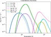 |
Fig. 1. Contribution functions for SPICE lines of interest computed using the CHIANTI database, version 11 (Dufresne et al. 2024). The solid lines represent calculations with a density of ne = 1 × 108 cm−3, the dotted lines correspond to ne = 1 × 109 cm−3, and the dashed lines to ne = 1 × 1010 cm−3. |
Two ARs were captured in the dataset from December 2022: NOAA 13171 and NOAA 13169. Both are registered as β-class ARs. Their characteristics are summarized in Table 1.
Technical description of observed ARs.
NOAA 13169 remained in SPICE’s field of view (FOV) the longest and is therefore the main focus of our analysis. The AR was first observed on December 17, 2022, already exhibiting a bipolarity in its sunspot structure. During SPICE observations, the AR was in its late, slow-emerging phase (see Figure 2). Its magnetic configuration was complex enough that opposite-polarity spots could not be clearly distinguished. Figure 3 shows the evolution of the AR seen in the SDO/AIA (Lemen et al. 2012) 171 Å band, along with the corresponding magnetograms from HMI (Scherrer et al. 2012). The latter are plotted within the range of ±200 G. The leading positive-polarity sunspot group remains consistent throughout the observations, bordered on its west side by a negative, more dispersed field.
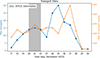 |
Fig. 2. Evolution of AR 13169 in terms of sunspot number (blue curve) and sunspot area (orange curve). Data are the courtesy of https://www.spaceweatherlive.com. During this period, three M-class flares and 61 C-class flares were recorded. Observation times studied here are highlighted in gray. |
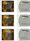 |
Fig. 3. Evolution of AR 13169 (top left in the first raster) from December 20–22, 2022. Left: SPICE Ne VIII 770 Å rasters overlaid on SDO/AIA 171 Å. Right: Corresponding SDO/HMI magnetograms with C III 977 Å rasters. On the magnetograms, green/(yellow) areas represent positive/(negative) polarity. Note: The dark horizontal lines (“dumbbells”) are square alignment apertures, located at each end of the slits. |
Two main outflows are seen in the Extreme Ultra-Violet (EUV) FOV. On December 22, a full loop can be observed within SPICE’s raster (see Figure 3, bottom panel). This loop seems to be newly formed, linking the strong positive magnetic field area to the negative area. Further confirmation of high magnetic activity is provided by the flares associated with the AR (on December 20, one M1.1-class flare at 13:59 UT and eight C-class flares were associated with AR13169).
To investigate plasma composition and dynamics within the observed AR, we now turn to the spectroscopic diagnostics and data processing methods used in this study.
3. Methods
Figure A.2 shows C III 977 Å, O VI 1032 Å and Ne VIII 770 Å radiance maps. All radiance maps were obtained by fitting the spectral lines with a Gaussian model, using sub-windows and multiple Gaussian curves (up to three) if several emission peaks were present in a single window (see Table 2). The average radiance values are presented in Table 3.
Lines extracted from the SPROUTS dataset.
Radiance values in milliwatts per square meter per steradian.
Note that the O II 718 Å and O VI 1032 Å are the only windows containing a single emission peak, while S IV 750 Å/Mg IX 749 Å, Ne VIII 770 Å and Ly-gamma-CIII windows contain two distinct emission peaks. The last three windows, O III 703 Å/Mg IX 706 Å, S V 786 Å/O IV 787 Å and N III 991 Å exhibit three emission lines.
To compute the relative FIP bias (the ratio of FIP bias of element X over element Y rather than H), we used three different line ratios covering different ranges of temperatures and thus different regions in the solar atmosphere: S V 786 Å(low-FIP proxy, 10.4 eV, log(T) = 5.2 K) and O IV 787 Å(high-FIP, 13.6 eV, log(T) = 5.2 K), covering the lower transition region; and Mg VIII 772 Å (low-FIP, 7.6 eV, log(T) = 5.85 K) and Ne VIII 770 Å (very-high FIP, 21.6 eV, log(T) = 5.8 K) as well as Mg IX 706 Å (low-FIP, 7.6 eV, log(T) = 5.9 K) and Ne VIII 770 Å, covering the lower corona. Even though sulfur is considered to be an intermediate-FIP, we still used it in our diagnostics to investigate the behavior of this ambiguous element, noting that it exhibits different behaviors based on magnetic configuration.
To account for differences in contribution function, as well as temperature and density effects, we included a differential emission measure (DEM) factor in our FIP bias computation. The DEM provides a measure of the amount of the emitting plasma along the line of sight as a function of temperature. We later derived DEMs from SPICE; however, DEM variance is too large for a reference DEM to be acceptable. Therefore, real computed DEMs should be used instead. The FIP bias is numerically computed as
 (2)
(2)
where LF and HF respectively denote low-FIP and high-FIP elements, and ⟨a ⋅ b⟩ designates the scalar product between a and b.
Determining the DEM from observed radiances in multiple spectroscopic lines is a challenging task due to the limitations of integral inversion methods, such as data insufficiency and the ill-conditioned nature of the problem, particularly in the density dimension (Craig & Brown 1976; Judge et al. 1997). Most DEM determination techniques require prior density measurements, and inversion methods often struggle to accurately resolve the general shape and finer details of the DEM, especially for multi-thermal plasmas, where solutions are biased to specific temperature ranges (Testa et al. 2012; Guennou et al. 2012). However, here we use Plowman & Caspi (2020)’s method, which enables a realistic estimation of the DEM directly from the same data used to compute the radiance, allowing for a consistent determination of the FIP bias as well. We checked that variations in the density chosen (here, ne = 109 cm−3) did not significantly affect the contribution function. Once the DEM estimates are computed, they are used in Equation (2).
Figure 4 presents the emission measure (EM) loci and the DEM results for the right footpoint of AR 13196 on December 21, 2022 at 03:34 UT. The EM loci intersect at logT = 5.8 K, confirmed by the DEM showing that most of the contribution originates from material around logT = 5.8 K, even though contributions from other temperatures are non-negligible. Neither the DEM nor the contribution functions show strong density dependency for the lines used. A detailed explanation on how the uncertainties (green- and orange- shaded areas) are computed for this study is presented in Appendix B.
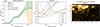 |
Fig. 4. DEM estimation (left panel), EM loci (middle panel; providing an upper-limit estimate of the DEM) and corresponding zone on the Ne VIII 770 Å map. The DEM estimation indicates a rather multi-thermal emission. The dotted gray lines indicate the range of temperature where the DEM estimation is reliable, and the different line styles represent different densities. Note: The scale for the DEM is linear. |
Now that we have established the methods used, these diagnostics are applied to derive and investigate the spatial and temporal changes in the FIP bias.
4. Results
Different diagnostics, involving a wide range of temperatures and ionization energies, have been computed. The ratios corresponding the to different solar atmospheric layers were computed using the methods described in Section 3.
AR 13169 was tracked by using several macropixels, designated as the color boxes in Figure 5. Since the rasters were recorded over several hours, the boxes follow the rotation of the Sun rather than the specific features of the AR at a given time.
The five distinctly colored boxes (regions) have the following properties for the three-day time series: 1) All remain within the raster bounds with sufficient signal-to-noise ratios to illustrate FIP bias behaviors. 2) Each similarly colored box (region) represents a targeted evolving feature within the AR. Region 1 (blue) is targets the AR footpoint; region 2 (orange) represents the core of the AR; regions 3, 4 and 5 (green, red and purple, respectively) represent fan loops, at varying distances from the core. In the right column of Fig. 5, the marker colors correspond to the tracked regions. According to fractionation models, the footpoints lie where most of the fractionation occurs; fan loops are more likely subject to interchange reconnection, and the AR core has the most dynamic, unpredictable environment. While the FIP bias maps were calculated on a pixel-by-pixel basis, we used the average spectrum over the selected region to reduce the uncertainties in the right-most panel, which exhibits a more quantitative FIP bias estimate.
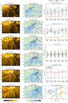 |
Fig. 5. Evolution of AR 13169 with time progressing downward. Left column: SPICE radiance maps seen in the Ne VIII 770 line |
Tracking results are shown in Figure 5. We begin by discussing the middle panels (i.e., the Mg VIII/Ne VIII maps), followed right-column panels, and finally an analysis of potential mechanisms at play.
The FIP bias maps seen in the Mg VIII/Ne VIII ratio show the spatial distribution of the FIP bias within the AR well. Whereas the core is mainly photospheric, the footpoints, fan loops, and boundaries (especially the right-hand one) exhibit strong fractionation. Over the course of two days, the FIP bias seems to increase and intensify at the AR footpoint, between regions 1 and 3. These maps allow us to differentiate between regions where we can observe an enhancement of the different abundance ratios. They inform our selection of regions to study quantitatively. This is illustrated in the plots on the right-hand panel:
Mg VIII/Ne VIII: Region 2 (orange curve) exhibits photospheric-like abundances at the start of the observations, showing a slow increase over time. The values from the AR core are close to the quiet-Sun reference, then shift toward coronal abundances. The macropixels targeting the AR boundary and fan loops, however, exhibit coronal-like abundances, especially those close to the bright core, with a global increasing trend from around 2.5 to above 3.5 after two days, except for region 5, which is the furthest from the core.
Mg IX/Ne VIII: All regions show similar behavior to Mg VIII/Ne VIII, but with greater variation in values, discussed below.
S V/O IV: This diagnostic is particularly interesting because both lines are close in wavelength and temperature yet exhibit a substantial FIP gap and good signal-to-noise ratio. All regions show highly correlated trends and similar values, starting near photospheric figures and showing a slight increase over the observation period.
Overall, the ratios show either a consistent, slow increase in the FIP bias over time or stay constant at coronal values. The slow increase in FIP bias matches AR 13169’s slow-emerging phase, during which waves are trapped and resonate within the loop. The results suggest that the resonant frequency of the loop does not change dramatically; therefore, the waves have a chance to remain in resonance. The structure-dependent evolution of the FIP bias in most ratios aligns with the findings of Warren et al. (2016) that intense heating events exhibit near-photospheric composition, while more stable structures such as coronal “fans” show typical coronal composition.
An important caveat, as shown in the bottom-right plot of Figure 5, is the dependence of the inferred FIP bias on the ratio of contribution functions. For the Mg/Ne and S/O pairs, the ratio of contribution functions varies noticeably with temperature. While it remains relatively constant over the range considered for S/O and Mg VIII/Ne VIII, Mg IX/Ne VIII exhibits stronger temperature dependence. This sensitivity partly reflects an instrumental limitation of SPICE, as the relevant lines peak at different temperatures and the DEM becomes poorly constrained above  when only high-FIP lines are available. Consequently, some of the apparent variations in the Mg/Ne ratios may be partly thermal in origin rather than purely compositional. The impact of this temperature dependence on the derived FIP bias is mitigated through the use of the DEM in the computation, rather than relying solely on the direct ratio of the contribution functions.
The boundaries and fan loops of the AR exhibit on average much higher fractionation. The most likely explanation is interchange reconnection between open field lines, with photospheric abundance reconnecting with coronal-abundance loops, thereby enriching the coronal composition at the boundaries. Another phenomenon we may be observing is the dynamic AR core, where emerging loops fill quickly with photospheric abundances (chromospheric plasma) and become fractionated over time. The high values at the fan loops and footpoints could be the signature of fractionated plasma that remains at the top of the loops for a few hours, before cooling and draining back down along the loop charged with coronal abundances.
The enhancement of sulfur compared to O denotes a low-FIP behavior from S. This trend is specifically notable at the footpoints of loops. Kuroda & Laming (2020) suggested that the enhancement of intermediate-FIP elements took place in the lower chromosphere, where H is not ionized. This phenomenon is even more pronounced in areas where non-resonant waves are present, a characteristic of open-field regions.
5. Modeling
Following the model developed in Laming (2017), Laming et al. (2019), FIP fractionation was estimated for the AR observed. This model describes the observed fractionation of elemental abundances in the solar atmosphere at a low time resolution, i.e. ignoring the potential bursts of fractionation caused by nanoflares for long-lived structures such as coronal loops, ARs, and solar wind outflow regions. Within these static scenarios, fractionation in closed loops is thought to take place in the upper chromosphere.
The ponderomotive force acts primarily on the low-FIP elements, which have a significantly higher ionization fraction than the high-FIP elements (see the middle and right panels at the top of Figure 6). This force preferentially lifts them toward the top of the transition region. Upon reaching this region, two key changes occur: the temperature rises enough to fully ionize both low- and high-FIP elements, eliminating the distinction between ions and neutrals, and the density gradient decreases, causing the effects of the ponderomotive force to vanish. As a result, the fractionation process ceases at the transition region’s upper boundary, locking in the established fractionation pattern. Other mechanisms then are thought to transport the fractionated plasma into the corona.
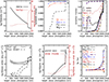 |
Fig. 6. Top panels, from left to right: Chromospheric density and temperature structures, low FIP ionization fractions and high FIP ionization fractions. Bottom panels, from left to right: Wave energy fluxes, ponderomotive acceleration, slow mode wave amplitudes, and fractionations with height in the chromosphere. While the Fe/O ratio increases, the S/O does not. This behavior is typical of resonant waves on closed loops. |
The parameters consist of an 80 000 kilometer-long loop with a 100 G magnetic field. These values are rough estimates inferred from AIA images. Waves have angular frequencies of 0.332 rad/s and 0.665 rad/s (fundamental and first harmonic), with amplitudes chosen to give FIP fractionations around 4 with respect to oxygen.
The modeled FIP fractionation values are represented in Figure 6. The key feature is in the right panel, where low-FIP elements start to behave significantly differently with respect to the high-FIP elements in the upper chromosphere. The intermediate element sulfur, which presumably behaves as a high-FIP element in closed magnetic structures (see Baker et al. 2024 and references therein), remains at a constant ionization rate. However, it is interesting to note that in the ponderomotive force model, S behaves qualitatively as a low-FIP element relative to O, being enhanced rather than depleted at a chromospheric altitude of 220 km, albeit not by very much (see Figure 6).
Overall, the data matches the model, similarly to Mihailescu et al. (2023)’s work, where they also compared the ponderomotive force model to Hinode/EIS observations. Comparing the model to Figure 5, the modeled (final) FIP bias for Mg/Ne is 3.20, and S/O shows a modest value of 1.26. The S/O observations and model show the best agreement, while the Mg/Ne ratios are consistent mostly with regions 1,3 and 4 (AR boundary).
Despite the discrepancies remaining between the models and observations of abundance changes, both have converged more closely in recent years. These first SPICE SPROUTS raster results suggest that fractionation occurs at chromospheric levels and that the fractionated plasma is brought at the top of the transition region after a time delay of about 24 hours. Understanding the differences between FIP bias diagnostics and the fractionation mechanisms for S will be crucial for linking in situ plasma observations to their solar surface origin, as S is frequently observed in both remote sensing and in situ FIP bias diagnostics.
6. Discussion
Investigating the FIP effect and its evolution with respect to different variables is essential for understanding the fractionation mechanisms of photospheric plasma. From SPICE’s observations and our diagnostics, we can conclude that waves are highly likely to cause fractionation. The Mg/Ne increases is expected if the waves causing the fractionation resonate with the coronal loop, which almost certainly means they are generated in the coronal part of the loop – subject to the boundary conditions at the loop footpoints – analogous to an optical resonating cavity. Plasma mixing, interchange reconnection, flux emergence and cancellation are important factors in the observed values of FIP bias (Koukras et al. 2025; Testa et al. 2023).
We base our conclusions solely on Mg VIII/Ne VIII and S V/O IV. The differences between the two Mg/Ne ratios may stem from a slight temperature mismatch: Mg VIII and Ne VIII are formed at similar temperatures and have similar wavelengths, whereas Mg IX forms at a higher temperature, near the upper limit of SPICE’s sensitivity. To better constrain the higher-temperature lines, coordinated observations with Hinode/EIS and SPICE are ideal (Brooks et al. 2022, 2024).
During the emergence phase (early in the study), the spectra could be affected by absorption from intervening H I, whereas later spectra are not, presumably because enough of the loop has emerged to sufficiently higher altitudes. This mainly affect the C III 977 and N III 991 lines, which lie shortward of the H I edge at 912 Å and can be absorbed (Orrall & Schmahl 1976). Mg VIII/Ne VIII and S V/O IV are likely unaffected by this phenomenon, because these lines are close in wavelength, causing H I absorption to affect them equally with no impact on the FIP bias computation. The Mg IX 706/Ne VIII 770 ratio has H I absorption cross sections of 3.2 and 4.0 Mb respectively; thus selective absorption of Ne VIII 770 over Mg IX 706 in a neutral hydrogen column density of 1.25 × 1018 cm−2 could give rise to an “apparent FIP effect”. However, there is no evidence for such an H column in any of the images, and uncertainties in the DEM reconstruction (see Figure 4, left panel) are a more likely source of uncertainty.
Observing different behaviors for different magnesium lines could be explained by the differences in temperature and therefore contribution functions, which are a crucial part of estimating DEMs and computing the FIP bias. Further observations and analysis would help assess which ratio is the most reliable, noting that Mg IX usually has a better signal-to-noise ratio, but Mg VIII has a temperature and wavelength closer to those of Ne VIII.
In their study, Widing & Feldman (2001) postulated that coronal loops emerge with photospheric abundances – and only become coronal-abundant when at least a part of the loop reaches the corona. With this postulate and recent results, including the observations made in this work, the FIP effect observed in this scenario is likely caused by a cascade of events originating in the corona.
The slow temporal evolution over timescales of tens-of-hours to days suggests steady heating; nevertheless, more chaotic evolution within smaller timescales is likely to occur. Outflow regions maintain consistently high FIP bias throughout the observation period as observed by Testa et al. (2023). They found a moderate correlation (Pearson’s correlation of 0.35 for their dataset) between the chromospheric turbulence inferred from IRIS and the high FIP bias values at the boundary of the AR, similar to what we observe with the lower temperature lines from SPICE. However, in contrast to the coronal-like values reported by Testa et al. (2023), our diagnostics predominantly yield photospheric abundance values in the AR core, even though both studies reveal a similarly stable temporal trend.
In Figure 5 AR 13169 is slowly emerges. We infer that the waves in the magnetic field are trapped within the structure and resonate, as in an optical resonant cavity, giving the FIP bias time to develop and increase. Looking at the evolution of the magnetic structure over the time period studied, we observe numerous flux cancellation events around the right footpoint of AR 13169. These phenomena could lead to the emergence of new photospheric flux, explaining the lower values observed in Figure 5. Combining SPICE observations with models, it appears that the FIP bias also depends on height in the chromosphere and lower transition region. However, once the plasma reaches the transition region, most of the fractionation has occurred, and subsequent evolution is very slow. The S V/O IV ratio indicates the presence of resonant waves on the transition region temperature structures, and these waves must be generated in the corona.
Limitations of the method The interpretation of the SPICE- derived FIP bias values involves several sources of uncertainty. Uncertainties exist in the data itself, which must be propagated through line fitting and DEM estimation. Contribution functions also carry their own uncertainties. Although the data suggest a slow temporal evolution of the FIP bias, this trend cannot be confirmed with certainty due to limited cadence and possible height-dependent effects in the chromosphere and transition region. A detailed explanation of how we address these uncertainties and quantify them can be found in Appendix B. Temperature and shape mismatch in the contribution functions may also contribute to differences in the inferred FIP bias, especially for Mg IX which forms at higher temperatures near the upper sensitivity limit of SPICE. During the emergence phase (early in the study) spectra may have been affected by H I absorption for lines shortward of 912 Å. However, no clear evidence of large neutral hydrogen columns is found; moreover, once the loops are established, this effect should be minimized.
It is beyond the scope of this paper to quantitatively relate the rate of temperature increase to the product of wave energy and damping rate. Indeed, there is currently no consensus on the dominant wave damping mechanisms or their efficiencies. Coronal loops can be heated by episodic events such as nanoflares (Dahlburg et al. 2016), which can in turn excite Alfvén waves. This modulation of the Alfvén wave spectrum likely influences the ponderomotive force responsible for FIP fractionation. While individual nanoflares occur on timescales of minutes, the resulting changes in the wave environment and ion–neutral coupling in the chromosphere could act cumulatively, producing observable compositional evolution on much longer timescales (tens of hours to days).
Finally, the derived FIP bias values depend on assumptions about plasma homogeneity, ionization equilibrium, and accurate line formation modeling, with uncertainties propagating from data reduction through DEM estimation. Despite these limitations, the observed trends remain meaningful and provide valuable insights when considered alongside models and complementary observations.
7. Conclusion
These SPICE SPROUTS observations provide needed insight into the evolution of the FIP bias, specifically as we look deeper in the atmosphere to investigate the chromospheric origin of plasma fractionation. The high number of spectral lines recorded and the recurrent recordings enable us to follow the fractionation of elements from the chromosphere to the corona over time.
We investigated the variability in FIP bias during the emergence phase of AR 13169. We found clear evidence of resonant waves generated in the corona at the boundaries and footpoints of the AR, as well as in in the transition region lines. From this study, we conclude that resonant waves are the principal driver of FIP fractionation at the transition region. We also observe a gradual evolution over time and across AR structures.
A broader motivation for this work arises from the fundamental question of wave origin within the context of the ponderomotive force model of FIP fractionation. Given this model, the next key step is to determine where the responsible waves originate. The distinction between resonant and nonresonant waves, as inferred from sulfur behavior, appears to favor resonant waves and thus supports a coronal origin. A more direct line of reasoning, however, comes from the observations of Widing & Feldman (2001), who found that FIP fractionation begins to develop only after coronal loops have extended into the corona. If the source of the relevant waves were located lower in the atmosphere, such as the photosphere, loops would be expected to emerge already exhibiting FIP fractionation. The Widing & Feldman (2001) study remains limited in scope, however, and warrants further investigation and replication.
We suggest that future SPICE SPROUTS investigations prioritize the Mg/Ne and S V/O IV ratios as key diagnostics, even though we draw attention to the potential strong temperature effects on the FIP bias, especially for the magnesium lines.
Coupling SPICE’s observations with high-resolution EUV imaging from Solar Orbiter’s EUI (Rochus et al. 2022) – unfortunately unavailable at the time of these observations – could provide insightful material to discriminate regimes of FIP fractionation, i.e., whether the observed plasma fractionates low or high in the chromosphere and its associated mechanisms. The SWA/HIS instrument (Owen et al. 2020), part of SolO’s in situ suite, could also offer connectivity and further confirmation of solar wind streams emerging from the regions studied.
This study focuses on a specific subset of SPROUTS observations to establish a robust methodological framework for these novel observations. Future studies will build upon this foundation and incorporate data from other solar observatories. In future work, we plan to extend our analysis to include a broader range of data sources pertaining to this AR and the slow solar wind possibly emanating from its eastern boundary.
Further investigation into the evolution of this AR can be achieved by utilizing observations from other missions. The Extreme-Ultraviolet Imaging Spectrometer (Culhane et al. 2007) on board the Hinode (Kosugi et al. 2007) mission observed the AR in the days following the SPICE observations. Measurements of Doppler velocities, densities, and other abundance diagnostics could provide additional context as well as insights into the AR’s continued evolution. Using the Polarimetric and Helioseismic Imager (PHI) (Solanki et al. 2020) and advanced modeling, we can extrapolate the coronal magnetic field. This would allow us to better visualize the magnetic structure of the AR itself and understand its interrelationship with the structures observed in the EUV images, as the Sun’s magnetic field drives the dynamics and structure of the solar corona. Magnetic field extrapolations also help determine where the plasma reaching Solar Orbiter originates. Combining these model predictions with the analysis of in situ data would give us a clearer idea if the plasma from this AR would eventually reach the spacecraft through reconnection at the boundary with the coronal hole to the south. Notably, SWA-HIS (Owen et al. 2020), which measures heavy ion abundances in the solar wind, recorded data in the days following these spectroscopic observations and the data are now available. In addition to these efforts, other datasets of SPROUTS observations will allow us to further explore temporal changes in a wider variety of solar structures.
Acknowledgments
The authors would like to thank the referee for their very insightful comments and suggestions. These efforts at SwRI for Solar Orbiter SPICE are supported by NASA under GSFC subcontract #80GSFC20C0053 to Southwest Research Institute. The development of the SPICE instrument has been funded by ESA member states and ESA (contract no. SOL.S.ASTR.CON. 00070). J.M.L. was funded by basic research funds of the Office of Naval Research. N.Z.P. is supported by STFC Consolidated Grant ST/W001004/1. Solar Orbiter is a space mission of international collaboration between ESA and NASA, operated by ESA. The development of SPICE has been funded by ESA member states and ESA. It was built and is operated by a multi-national consortium of research institutes supported by their respective funding agencies: STFC RAL (UKSA, hardware lead), IAS (CNES, operations lead), GSFC (NASA), MPS (DLR), PMOD/WRC (Swiss Space Office), SwRI (NASA), UiO (Norwegian Space Agency). This research used the open source sospice (https://github.com/solo-spice/sospice) Python package, Fiasco (Barnes et al. 2024), the CHIANTI database version 11 (Dufresne et al. 2024), Astropy and Sunpy.
References
- Baker, D., Brooks, D. H., Démoulin, P., et al. 2013, ApJ, 778, 69 [NASA ADS] [CrossRef] [Google Scholar]
- Baker, D., Brooks, D. H., Démoulin, P., et al. 2015, ApJ, 802, 104 [NASA ADS] [CrossRef] [Google Scholar]
- Baker, D., Brooks, D. H., van Driel-Gesztelyi, L., et al. 2018, ApJ, 856, 71 [Google Scholar]
- Baker, D., Green, L. M., Brooks, D. H., et al. 2022, ApJ, 924, 17 [NASA ADS] [CrossRef] [Google Scholar]
- Baker, D., van Driel-Gesztelyi, L., James, A. W., et al. 2024, ApJ, 970, 39 [NASA ADS] [CrossRef] [Google Scholar]
- Barnes, W., Stansby, D., Murphy, N., et al. 2024, https://doi.org/10.5281/zenodo.10612118 [Google Scholar]
- Brooks, D. H., Janvier, M., Baker, D., et al. 2022, ApJ, 940, 66 [NASA ADS] [CrossRef] [Google Scholar]
- Brooks, D. H., Warren, H. P., Baker, D., Matthews, S. A., & Yardley, S. L. 2024, ApJ, 976, 188 [Google Scholar]
- Craig, I. J. D., & Brown, J. C. 1976, A&A, 49, 239 [NASA ADS] [Google Scholar]
- Culhane, J. L., Harra, L. K., James, A. M., et al. 2007, Sol. Phys., 243, 19 [Google Scholar]
- Dahlburg, R. B., Laming, J. M., Taylor, B. D., & Obenschain, K. 2016, ApJ, 831, 160 [CrossRef] [Google Scholar]
- De Pontieu, B., Title, A. M., Lemen, J. R., et al. 2014, Sol. Phys., 289, 2733 [Google Scholar]
- Doschek, G., Warren, H., & Feldman, U. 2015, ApJ, 808, L7 [NASA ADS] [CrossRef] [Google Scholar]
- Dufresne, R. P., Del Zanna, G., Young, P. R., et al. 2024, ApJ, 974, 71 [Google Scholar]
- Giammanco, C., Wurz, P., Opitz, A., Ipavich, F. M., & Paquette, J. A. 2007, AJ, 134, 2451 [Google Scholar]
- Guennou, C., Auchère, F., Soubrié, E., et al. 2012, ApJS, 203, 25 [NASA ADS] [CrossRef] [Google Scholar]
- Judge, P. G., Hubeny, V., & Brown, J. C. 1997, ApJ, 475, 275 [NASA ADS] [CrossRef] [Google Scholar]
- Ko, Y.-K., Young, P. R., Muglach, K., Warren, H. P., & Ugarte-Urra, I. 2016, ApJ, 826, 126 [Google Scholar]
- Kosugi, T., Matsuzaki, K., Sakao, T., et al. 2007, Sol. Phys., 243, 3 [Google Scholar]
- Koukras, A., Savin, D. W., & Hahn, M. 2025, ApJ, 982, 173 [Google Scholar]
- Kuroda, N., & Laming, J. M. 2020, ApJ, 895, 36 [Google Scholar]
- Laming, J. M. 2015, Liv. Rev. Sol. Phys., 12, 2 [Google Scholar]
- Laming, J. M. 2017, ApJ, 844, 153 [Google Scholar]
- Laming, J. M. 2021, ApJ, 909, 17 [NASA ADS] [CrossRef] [Google Scholar]
- Laming, J. M., Drake, J. J., & Widing, K. G. 1995, ApJ, 443, 416 [Google Scholar]
- Laming, J. M., Vourlidas, A., Korendyke, C., et al. 2019, ApJ, 879, 124 [Google Scholar]
- Lanzafame, A. C., Brooks, D. H., Lang, J., et al. 2002, A&A, 384, 242 [NASA ADS] [CrossRef] [EDP Sciences] [Google Scholar]
- Lemen, J. R., Title, A. M., Akin, D. J., et al. 2012, Sol. Phys., 275, 17 [Google Scholar]
- Meyer, J. P. 1985, ApJS, 57, 173 [CrossRef] [Google Scholar]
- Meyer, J.-P. 1991, Adv. Space Res., 11, 269 [Google Scholar]
- Mihailescu, T., Baker, D., Green, L. M., et al. 2022, ApJ, 933, 245 [NASA ADS] [CrossRef] [Google Scholar]
- Mihailescu, T., Brooks, D. H., Laming, J. M., et al. 2023, ApJ, 959, 72 [Google Scholar]
- Müller, D., St. Cyr, O. C., Zouganelis, I., et al. 2020, A&A, 642, A1 [Google Scholar]
- Orrall, F. Q., & Schmahl, E. J. 1976, Sol. Phys., 50, 365 [Google Scholar]
- Owen, C. J., Bruno, R., Livi, S., et al. 2020, A&A, 642, A16 [EDP Sciences] [Google Scholar]
- Plowman, J., & Caspi, A. 2020, ApJ, 905, 17 [NASA ADS] [CrossRef] [Google Scholar]
- Plowman, J., Barnes, W. T., Caspi, A., & Cheung, M. 2020, https://doi.org/10.5281/zenodo.6604713 [Google Scholar]
- Reames, D. V. 2018, Sol. Phys., 293, 47 [Google Scholar]
- Réville, V., Rouillard, A. P., Velli, M., et al. 2021, Front. Astron. Space Sci., 8, 2 [Google Scholar]
- Rochus, P., Auchère, F., Berghmans, D., et al. 2022, A&A, 665, C1 [NASA ADS] [CrossRef] [EDP Sciences] [Google Scholar]
- Scherrer, P. H., Schou, J., Bush, R. I., et al. 2012, Sol. Phys., 275, 207 [Google Scholar]
- Schmelz, J. T., Reames, D. V., von Steiger, R., & Basu, S. 2012, ApJ, 755, 33 [NASA ADS] [CrossRef] [Google Scholar]
- Sheeley, N. R., Jr. 1995, ApJ, 440, 884 [NASA ADS] [CrossRef] [Google Scholar]
- Solanki, S. K., del Toro Iniesta, J. C., Woch, J., et al. 2020, A&A, 642, A11 [NASA ADS] [CrossRef] [EDP Sciences] [Google Scholar]
- Testa, P., De Pontieu, B., Martínez-Sykora, J., Hansteen, V., & Carlsson, M. 2012, ApJ, 758, 54 [NASA ADS] [CrossRef] [Google Scholar]
- Testa, P., Martínez-Sykora, J., & De Pontieu, B. 2023, ApJ, 944, 117 [Google Scholar]
- To, A. S., Long, D. M., Baker, D., et al. 2021, ApJ, 911, 86 [NASA ADS] [CrossRef] [Google Scholar]
- Varesano, T., Hassler, D. M., Zambrana Prado, N., et al. 2024, A&A, 685, A146 [NASA ADS] [CrossRef] [EDP Sciences] [Google Scholar]
- Warren, H. P., Brooks, D. H., Doschek, G. A., & Feldman, U. 2016, ApJ, 824, 56 [NASA ADS] [CrossRef] [Google Scholar]
- Widing, K. G. 1997, ApJ, 480, 400 [NASA ADS] [CrossRef] [Google Scholar]
- Widing, K. G., & Feldman, U. 2001, ApJ, 555, 426 [Google Scholar]
- Young, P. R., & Mason, H. E. 1997, Sol. Phys., 175, 523 [Google Scholar]
- Zambrana Prado, N., & Buchlin, É. 2019, A&A, 632, A20 [NASA ADS] [CrossRef] [EDP Sciences] [Google Scholar]
Appendix A: Spectra and radiance maps
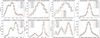 |
Fig. A.1. Average spectra over the footpoint of AR 13169, computed over an area of 15x30 pixels. Each color represents a different observation time. |
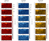 |
Fig. A.2. Radiance map closeups seen in the C III 977 Å, O VI 1032 Åand Ne VIII 770 Ålines from December 20-22 2022. The field of view is focused on AR 13169 (upper parts of the panels). Time progresses as shown in Figure 5. |
Appendix B: Uncertainty computation
B.1. Radiance uncertainty
We focus here on the lines that were used for the FIP bias computation, but the method applies for every lines. For the O III 703 Å/ Mg IX 706 Å, S V 786 Å/ O IV 787 Åand N III 991 Åwindow, we used triple Gaussian fitting with a uniform background. All centroids, amplitudes, and widths of the lines were free parameters with bounds, as well as the uniform background, since this set of three blended lines typically has enough signal-to-noise ratio for the lines to be easily identified and separated. The Ne VIII 770 Å/ Mg VIII 772 Åand C III 977 Åwindow have been fitted with two gaussians, on the same methodology as the three-gaussian window.
We compute the radiances by passing initial guesses to a bounded nonlinear least squares fitting routine (curve_fit). From the best-fit parameters, the integrated radiance is calculated using the formula for the area under a Gaussian curve:
where A is the fitted amplitude and σ the standard deviation. This approach ensures a consistent and robust estimate of the total emission in each spectral feature, which is critical for the subsequent derivation of temperature diagnostics and FIP bias.
The uncertainties associated with radiances are estimated by propagating the errors from the spectral line fitting through each step of the calculation. Instrument-related errors from the sospice2 package are embedded in the line fitting routine with the sigma parameter of the curve_fit routine. The radiance uncertainty for each fitted spectral line is then derived from the covariance matrix output. Specifically, the uncertainty on the integrated line intensity is computed using the formula for error propagation of a Gaussian:
![Mathematical equation: $$ \delta I = \sqrt{2\pi } \left[ (\sigma \cdot \delta A) + (A \cdot \delta \sigma ) \right] $$](/articles/aa/full_html/2026/02/aa54166-25/aa54166-25-eq7.gif)
where A is the line amplitude, σ is the Gaussian width, and covA, σ is their covariance.
B.2. DEM uncertainty
The DEM forward problem is the same as in Plowman & Caspi (2020). Di are the data and σi their associated uncertainties. Ri are the contribution functions. Mi is the model fit to the data, and cj are the unknown coefficients of the DEM solution. Here we discuss the DEM uncertainty estimation method used in this paper which was first made public in the EMToolKit Github (Plowman et al. 2020).
To estimate the level of uncertainty in the DEM estimation, we need to evaluate the following: given a solution that satisfies Mi = Di, how much can the coefficients cj vary – resulting in a perturbed model M′i = ∑jRij(cj + Δcj) – before the modified solution reaches a given threshold χ′2, which is typically the number of data points (‘reduced’ χ′2 = 1).
This question can have multiple interpretations, each yielding a different estimate of uncertainty. One may ask how much a single coefficient cj can change, or how much all coefficients can vary collectively. The parameters could change coherently (e.g., all increasing or decreasing together), incoherently (e.g., in random directions), or in ways that compensate for each other. These scenarios produce very different results: fully compensating changes may yield formally infinite or undefined uncertainties, while coherent variation produces relatively small uncertainties. Incoherent or random variation lies in between and generally scales with the square root of the number of parameters.
For a more conservative estimation, a "one-parameter-at-a-time" approach is adopted: each cj is varied individually while holding others fixed. This yields the most straightforward and robust uncertainty estimate without requiring detailed knowledge of the solution.
Let Δcj be the only source of deviation from agreement (meaning that the other c in the coefficient vector stay constant) then χ′2 = ndata implies that
We can then estimate the errors as
Considering original contribution functions, Rij = ∫Ri(T)Bj(T) dT For the uncertainty estimate, we take the basis functions to be top hats of width Δlog10T = 0.1 K at temperature Tj (this is distinct from the width of the basis functions used for estimating the DEM, and should generally be taken to be of order the temperature resolution of the instrument). Thus Rij = Ri(Tj)Δlog10T and the uncertainty in a DEM component with that characteristic width is:
σEj is the uncertainty estimate we use in this paper. Correlated fluctuations in unresolved temperature elements can of course be higher, as is also the case in (for example) imaging observations.
B.3. FIP bias uncertainty
The FIP bias uncertainty is estimated by propagating the uncertainties in the intensities and contribution functions through the FIP bias equation (see Eq. 2). Since the FIP bias is computed on the average spectrum over a given zone, the radiance and DEM uncertainties are normalized by the size of the zone. The propagated error δFIP on the relative FIP bias is computed as:
with
 (B.1)
(B.1)
The error margin on the contribution functions (δCHF/LFi) has been taken as 15% of their value.
This approach incorporates the uncertainties in radiance measurements, DEMs and contribution functions into the final FIP bias uncertainty.
All Tables
All Figures
|
Fig. 1. Contribution functions for SPICE lines of interest computed using the CHIANTI database, version 11 (Dufresne et al. 2024). The solid lines represent calculations with a density of ne = 1 × 108 cm−3, the dotted lines correspond to ne = 1 × 109 cm−3, and the dashed lines to ne = 1 × 1010 cm−3. |
| In the text | |
|
Fig. 2. Evolution of AR 13169 in terms of sunspot number (blue curve) and sunspot area (orange curve). Data are the courtesy of https://www.spaceweatherlive.com. During this period, three M-class flares and 61 C-class flares were recorded. Observation times studied here are highlighted in gray. |
| In the text | |
|
Fig. 3. Evolution of AR 13169 (top left in the first raster) from December 20–22, 2022. Left: SPICE Ne VIII 770 Å rasters overlaid on SDO/AIA 171 Å. Right: Corresponding SDO/HMI magnetograms with C III 977 Å rasters. On the magnetograms, green/(yellow) areas represent positive/(negative) polarity. Note: The dark horizontal lines (“dumbbells”) are square alignment apertures, located at each end of the slits. |
| In the text | |
|
Fig. 4. DEM estimation (left panel), EM loci (middle panel; providing an upper-limit estimate of the DEM) and corresponding zone on the Ne VIII 770 Å map. The DEM estimation indicates a rather multi-thermal emission. The dotted gray lines indicate the range of temperature where the DEM estimation is reliable, and the different line styles represent different densities. Note: The scale for the DEM is linear. |
| In the text | |
|
Fig. 5. Evolution of AR 13169 with time progressing downward. Left column: SPICE radiance maps seen in the Ne VIII 770 line |
| In the text | |
|
Fig. 6. Top panels, from left to right: Chromospheric density and temperature structures, low FIP ionization fractions and high FIP ionization fractions. Bottom panels, from left to right: Wave energy fluxes, ponderomotive acceleration, slow mode wave amplitudes, and fractionations with height in the chromosphere. While the Fe/O ratio increases, the S/O does not. This behavior is typical of resonant waves on closed loops. |
| In the text | |
|
Fig. A.1. Average spectra over the footpoint of AR 13169, computed over an area of 15x30 pixels. Each color represents a different observation time. |
| In the text | |
|
Fig. A.2. Radiance map closeups seen in the C III 977 Å, O VI 1032 Åand Ne VIII 770 Ålines from December 20-22 2022. The field of view is focused on AR 13169 (upper parts of the panels). Time progresses as shown in Figure 5. |
| In the text | |
Current usage metrics show cumulative count of Article Views (full-text article views including HTML views, PDF and ePub downloads, according to the available data) and Abstracts Views on Vision4Press platform.
Data correspond to usage on the plateform after 2015. The current usage metrics is available 48-96 hours after online publication and is updated daily on week days.
Initial download of the metrics may take a while.