| Issue |
A&A
Volume 706, February 2026
|
|
|---|---|---|
| Article Number | A157 | |
| Number of page(s) | 27 | |
| Section | Planets, planetary systems, and small bodies | |
| DOI | https://doi.org/10.1051/0004-6361/202555631 | |
| Published online | 11 February 2026 | |
Accelerating exoplanet climate modelling
A machine learning approach to complement 3D general circulation model grid simulations
1
Space Research Institute, Austrian Academy of Sciences,
Schmiedlstrasse 6,
8042
Graz,
Austria
2
Institute for Theoretical Physics and Computational Physics, Graz University of Technology,
Petersgasse 16,
8010
Graz,
Austria
3
Institute of Physics, University of Graz,
Universitätsplatz 3,
8010
Graz,
Austria
★ Corresponding author: This email address is being protected from spambots. You need JavaScript enabled to view it.
Received:
22
May
2025
Accepted:
3
August
2025
Abstract
Context. With the development of ever-improving telescopes capable of observing exoplanet atmospheres in greater detail and number, there is a growing demand for enhanced three-dimensional climate models to support and help interpret observational data from space missions such as CHEOPS, TESS, JWST, PLATO, and Ariel. However, the computationally intensive and time-consuming nature of general circulation models (GCMs) poses significant challenges in simulating a wide range of exoplanetary atmospheres.
Aims. The aim of this study is to determine whether machine learning (ML) algorithms can be used to predict the three-dimensional temperature and wind structure of arbitrary tidally locked gaseous exoplanets in a range of planetary parameters.
Methods. We introduced a new three-dimensional GCM grid comprising 60 inflated hot Jupiters orbiting A, F, G, K, and M-type host stars, which we modelled using ExoRad. We defined four climate characteristics to characterise these planets: the dayside–nightside temperature difference, the evening–morning temperature difference, the maximum zonal wind speed, and the wind jet width. We trained a dense neural network (DNN) and an extreme gradient boosting algorithm (XGBoost) on this grid to predict local gas temperatures, as well as horizontal and vertical wind fields. To assess the reliability and quality of the ML models’ predictions, we selected WASP-121 b, HATS-42 b, NGTS-17 b, WASP-23 b, and NGTS-1 b–like planets, all of which are targets for PLATO observations, and modelled them using ExoRad and the two ML methods. For these test cases, we calculated the equilibrium gas-phase composition and transmission spectra to evaluate whether differences in local gas temperature between the general circulation model and ML approaches significantly affected the predicted chemical composition and transmission spectra.
Results. With the multi-layer neural network, that is DNN, predictions for the gas temperatures are to such a degree that the calculated spectra agree within 32 ppm for all but one planet, for which only one single HCN feature reaches a 100 ppm difference. The XGBoost predictions are somewhat worse but never exceed 380 ppm differences. Generally, the resulting deviations are too small to be detectable with the observational capabilities of modern space telescopes, including JWST. For the DNN, only the WASP-121 b-like planet, which is the hottest investigated planet, shows a general offset that is smaller than 16 ppm. Horizontal wind predictions are less accurate but can capture the most general trends. As with temperature, the DNN also outperforms XGBoost in this respect. Predicting vertical wind remains challenging for all ML methods that we explored in this study.
Conclusions. The developed ML emulators can, within one second, reliably predict the complete three-dimensional temperature field of an inflated warm to ultra-hot tidally locked Jupiter around A to M-type host stars. They therefore provide a fast and computationally inexpensive tool to complement and extend traditional GCM grids for exoplanet ensemble studies. The quality of the predictions is such that no, or only minimal, effects on the gas-phase chemistry and, consequently, on cloud formation and transmission spectra are expected.
Key words: astrochemistry / methods: data analysis / methods: numerical / planets and satellites: atmospheres / planets and satellites: gaseous planets
© The Authors 2026
 Open Access article, published by EDP Sciences, under the terms of the Creative Commons Attribution License (https://creativecommons.org/licenses/by/4.0), which permits unrestricted use, distribution, and reproduction in any medium, provided the original work is properly cited.
This article is published in open access under the Subscribe to Open model. This email address is being protected from spambots. You need JavaScript enabled to view it. to support open access publication.
1 Introduction
Exoplanet research is driven by a combination of discovering exoplanets to study their properties and evolution (e.g., Lissauer et al. 2023; Rauer et al. 2025; Reza et al. 2025) and by a detailed investigation of individual extrasolar planets. The aim is to understand, for example, their atmosphere chemistry and physics (e.g. Carone et al. 2025; Bell et al. 2024; Deline et al. 2025; Coulombe et al. 2023; Demangeon et al. 2024) or to prove the presence of an atmosphere (e.g. Rathcke et al. 2025). The gas giant extrasolar planets WASP-39 b (Espinoza et al. 2024, WASP-43 b (Hammond et al. 2024), HD 189733 b (Zhang et al. 2024), and WASP-107 b (Murphy et al. 2024) are among the first planets observed with JWST. JWST demonstrated that such gas giants exhibit day-night differences that may be traced by observing terminator asymmetries, as suggested by early models in Showman et al. (2020); Lee et al. (2015); Helling et al. (2016); von Paris et al. (2016); Line & Parmentier (2016), for example. The logical follow-up to this finding would be to utilise the exquisite data quality from JWST’s instruments to conduct comparative studies of an ensemble of gas giant exoplanets. The interpretation of the steadily increasing number of exoplanets to be characterised by JWST in combination with smaller telescopes, such as TESS and CHEOPS (e.g. Scandariato et al. 2024), requires simulations that model the relevant chemical and physical processes (gas dynamics, radiative transfer, gas phase chemistry, cloud formation). So far, a fully consistent 3D model atmosphere solution including clouds has been presented for only two gas giants: HD 189733b (Lee et al. 2016) and HD 209458 b (Lines et al. 2018.
One-dimensional atmosphere simulations allow for a wider variety of global parameters and hence a larger ensemble of objects, but they average out all horizontal atmosphere characteristics (e.g., Goyal et al. 2020; Morley et al. 2024; Jørgensen et al. 2024; Campos Estrada et al. 2025). The study of three-dimensional atmospheric and chemical structures was confined to the use of either cloud parametrisation (Parmentier et al. 2016; Komacek et al. 2022) or a hierarchical approach (Helling et al. 2023). Notably, both methods have a pre-defined set of model planets with set global parameters (planetary global temperature, host star, orbital distances, mass, element abundances).
The diversity of known exoplanets, even within the class of gas giants, is substantial, ranging from warm to ultra-hot. Classical grid studies are useful in revealing the underlying general principles of chemistry and climate dynamics, as in Carone et al. (2015); Kataria et al. (2016); Parmentier et al. (2016); Showman et al. (2020); Helling et al. (2023); Kennedy et al. (2025). By necessity, these studies only cover a small subset of global parameters, such as planetary and stellar radii and stellar effective temperatures, which makes them difficult to apply for detailed atmosphere characterisation of specific planets. In order to answer fundamental questions about the formation and evolution of exoplanet atmospheres in different galactic environments, the number of targets that undergo characterisation must increase (TESS: ca. 500, PLATO: ca. 200 (from Rauer et al. 2025)). Yield studies for the PLATO mission Matuszewski et al. 2023 suggest that a minimum of 800 new gas giants will be discovered with unprecedented precision in planetary radii (3%), which then require characterisation. The LOPS2 (long-pointing field southern hemisphere) field that will be first observed by PLATO contains a fair number of planets with vastly diverse properties (Sect. 3.4.1. in Nascimbeni et al. 2025).
Interpolating model atmosphere grids is a long-standing challenge for observers who wish to use these modelling data to help physically interpret their observational data (e.g., Sect. 4.1. in Petrus et al. 2024; Patience et al. 2012; Schmidt et al. 2016). An alternative is to apply highly parametrised model atmospheres and tune the parameters until observations fit (e.g., Schleich et al. 2024) or to train neural networks on spectral grids derived from forward models for fast data interpretation (e.g., Yip et al. 2024). Lueber et al. (2023) presents a study on one-dimensional profiles of brown dwarfs, consistently comparing calculated model atmospheres (though with parametrised clouds) with those derived from simplifying parametrisations used in their retrieval approach to validate what information can be deduced from such a rapid parametrisation that reproduces an observed spectrum.
In this present paper, we acknowledge the limits inherent to classical grid studies in general and in particular for three-dimensional atmosphere simulations, which may hamper rapid data interpretation for ensemble studies as well as for in-depth studies of specific planets since a pre-calculated atmosphere grid seldom contains the observed planet specifically (e.g., Patience et al. 2012; Petrus et al. 2024). Fig. 1 shows the planets that are current targets for the PLATO (green) and CHEOPS (dark red) missions, planets that JWST observed (gold), and a list of ideally suitable targets for exoplanet atmosphere studies collected by (Baxter et al. 2020) (grey). The coverage of the global planetary (Tglobal = 400 … 2600 K) and stellar effective temperature (Teff [K] for A, F, G, K and M host stars) of our new 3D AFGKM ExoRad (blue; introduced in Sect. 2) is shown for comparison. It covers well the overall global parameter range of the observational ensemble of gas giant planets, but not necessarily specific planets. For example, PLATO targets WASP-121 b, HATS-42 b, NGTS-17 b, WASP-23 b, or NGTS-1 b. These planets are explicitly highlighted with different colours, as they are used to test our machine learning (ML) predictions.
The study presented here is therefore dedicated to exploring the potential of ML as a reliable and time-efficient alternative to complex 3D GCM models for completing existing model grids (filling the gaps) and interpreting observational data. ML models are designed to predict the thermodynamic and hydrodynamic properties of exoplanetary atmospheres, which are critical to determining the chemical composition and, eventually, the observable transmission spectrum. This led us to explore the following research questions.
Can ML models predict the three-dimensional temperature and wind structure of un-modelled (unknown) exoplanet atmospheres?
Which ML models can efficiently fill the gaps in the grid? Do different ML models and methods provide consistent results? Can computational costs be reduced by using ML methods?
Do ML-predicted atmospheric structures differ from those obtained with traditional 3D GCM modelling (ExoRad)? How do these potential differences affect the chemical composition of the atmospheric gas as the necessary precursor for cloud formation? Would these differences be observable in a transmission spectrum?
We applied several ML models to the ExoRad 3D GCM model data to address the research questions posed in this study. We used a newly simulated ExoRad grid, introduced in Sect. 2, as the training data, as it represents the diversity of exoplanet atmospheres. We introduced four parameters to characterise the climate states of gas giants: the dayside–nightside temperature difference, the evening–morning terminator temperature difference, the wind jet speed, and the wind jet width (Fig. 5), to complement the global system parameters Teff, Tglobal, the orbital period (Porb), and the metallicity ([M/H]=0)). In Sect. 3, we outline our methodology, including the training and testing strategy that we applied to assess the ML model’s performance. In Sect. 4, we describe the ML models (e.g., DNN, XGBoost) employed in this work in detail. We present the results in Sect. 5, where we compare predictions from the ML models for unseen planets with ExoRad simulation results. This section further presents case studies of specific PLATO target gas giant exoplanets, demonstrating that ML models provide an efficient solution for filling gaps in 3D GCM atmosphere grids, making them a viable addition to integrate into data interpretation pipelines. In Sect. 5.2, we investigate how prediction errors from ML models propagate into the chemical equilibrium composition and transmission spectra. In Sect. 6, we discuss and compare the computational cost of ML models and ExoRad simulations. Finally, Sect. 7 presents our conclusions, including the result that a light-weight multi-layer neural network predicts local gas temperatures for unseen gas giant planets with a precision that is indistinguishable from that of the forward 3D GCM solution for the current observational facilities. The predictions are substantially more accurate than the differences between different GCM frameworks.
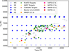 |
Fig. 1 3D ExoRad GCM grid of 60 simulated planets (blue) for different host stars from M to A (Teff [K], see Table A.1) and global planetary temperatures Tglobal [K]. Observation targets for JWST (yellow), PLATO (green), and CHEOPS (red) are overlaid. The hot Jupiters WASP-121 b, HATS-42 b, NGTS-17 b, WASP-23 b, and NGTS-1 b, highlighted in distinct colours, serve as test cases to evaluate the prediction accuracy of the ML models developed in this work. Grey points indicate objects from (Baxter et al. 2020). |
2 3D GCM grid ExoRad for gas giants orbiting M, G, K, F, and A stars
Three-dimensional (3D) climate grid studies have been extremely useful to explore the impact of diverse physical and chemical processes (e.g., kinetic chemistry (Komacek et al. 2019; Baeyens et al. 2021), photochemistry (Baeyens et al. 2022), and cloud distribution and ionisation states (Helling 2021)) for the warm to hot Jupiter population. Baeyens et al. (2021, 2022); Helling (2021) used the ExoRad 3D climate framework for hot Jupiters (Carone et al. 2020) with the dynamical core of MITgcm, employing Newtonian cooling to describe the irradiation of the tidally locked planets. In recent years, ExoRad was updated with expeRT/MITgcm to include complete radiative transfer and equilibrium gas phase chemistry (Schneider et al. 2022b,a). This new grid of 3D climate models provides the training data for the ML frameworks presented in this work.
2.1 Computational setup for 3D GCM grid
Star and planet setup: For comparability with previous work, the new grid assumes a moderately inflated Jupiter sized planet with RP = 1 RJup and g = 10 m/s2 similar to Baeyens et al. (2021, 2022); Helling et al. (2023), which yields a mass of 0.39 MJup. For the host stars, stellar parameters for M5V, KV5, GV5, F5V and A5V stars are adopted according to Pecaut & Mamajek (2013) (see Table A.1). We thus extend the grid towards planets around higher mass host stars. The setup is such that the tidally locked planets are placed at a semi major axis so that the global temperatures, Tglobal [K], averaged over the planet1 assumes values between 400 K and 2600 K in 200 K steps. The interior temperature, Tint [K], is determined via the parametric fit of Thorngren et al. (2019). For the planetary parameters (Tglobal [K], Tint [K], semi major axis a [au], and orbital period Porb [d]), please see Tables A.2–A.6.
Radiative transfer and chemistry set up: The gas opacities are implemented by correlated-k tabulated opacities combined in 11 spectral bins, corresponding to the S1 resolution in Schneider et al. (2022b) for the following species: H2O (from ExoMol2 – Tennyson et al. 2016, 2020), Na (Allard et al. 2019), K (Allard et al. 2019)3, CO2, CH4, NH3, CO, H2S, HCN, SiO, PH3 and FeH, as well as H− scattering suitable for an ionised atmosphere as listed in Schneider et al. (2022b, Table 1) excluding TiO and VO. Including them would create an upper atmosphere inversion for a subset of planets (Tglobal ≥ 1800 K). The grid is setup such to represent the impact of advection and irradiation with a similar chemical make-up, including major heating sources across a large range of global temperatures 400–2600 K. Collision-induced absorption for H2–H2 (Borysow et al. 2001; Borysow 2002; Richard et al. 2012) and H2–He (Borysow et al. 1988; Borysow & Frommhold 1989; Borysow et al. 1989), Rayleigh scattering for H2 (Dalgarno & Williams 1962), He (Chan & Dalgarno 1965), and H− free-free and bound-free opacities (Gray 2008) are included. Solar metallicity ([M/H] = 0) and a solar C/O ratio of 0.55 according to Asplund et al. (2009) are adopted for the planetary atmosphere chemistry calculated in LTE.
2.2 The 3D AFGKM ExoRad GCM grid
The 3D AFGKM ExoRad grid consists of 60 3D GCM models for gas giant exoplanets orbiting A, F, G, K, and M-type host stars (blue symbols in Fig. 1). The grid spans global planetary temperatures Tglobal = 400 … 2600 K. To introduce the new grid, we explored the selected one-dimensional gas pressure-temperature profiles for all these 60 grid planets (Fig. 2). The two-dimensional equatorial gas temperature maps for planets orbiting selected host stars (A, G, M; Fig. 3) demonstrate the change in local gas temperatures and atmospheric asymmetries that emerge from our 3D GCM simulations. The zonal wind speeds (Fig. 4), as drivers of the atmospheric asymmetries, are shown for the same set of host stars and planets. Lastly, in order to be able to characterise the climate state of the 60 3D AFGKM ExoRad GCM grid planets, we introduced four properties: day–night gas temperature difference, morning-evening gas temperature difference, maximum zonal wind speed and width of the wind jet4 (Fig. 5). These further allow for a comparison within the ensemble of gas giant planet climate states.
Atmospheric gas temperature–pressure: The global temperature asymmetries result from the interplay between advection (fluid dynamics) and host star irradiation, where the planet is subject to a strongly asymmetric irradiation field due to tidal locking, as it always faces its host star with the same side. The local gas temperature structure can also be strongly impacted by differences in planetary rotation. A planet with a given global temperature orbiting an M dwarf star is on a shorter orbital period with a faster tidally locked rotation rate compared to a planet with the same global temperature orbiting an A star (see Appendix A for the complete set of 3D GCM simulations).
Equatorial wind jets in gas giant exoplanets: Tidally locked warm and hot gas giant exoplanets develop a strong equatorial wind jet that efficiently transports warm dayside gases to the cold nightside. The changing gas temperature can cause observable asymmetries in the terminator. The equatorial jet changes depending on global system parameters (host star, orbital period; Fig. 4), resulting in the changing of local gas temperature distributions as shown in Fig. 3. The structure of the equatorial wind jet is diagnosed by displaying the maximum equatorial wind speed (bottom left) and the half-width of the equatorial jet (bottom right), that is, the latitudinal location at which the wind speed decreases to half of the maximum wind speed of the equatorial jet (Fig. 5). Day and night side temperature differences (top left, Fig. 5) further elucidate the efficiency of horizontal heat transport. Morning and evening terminator differences (top right, Fig. 5) are indicators for potential terminator asymmetries which will eventually be amplified by cloud formation (Helling et al. 2023; Helling 2021).
Climate state characteristics: The climate of each of the 60 AFGKM ExoRad grid 3D GCM models is characterised using four properties, as shown in Fig. 5: the day–night gas temperature difference (top left), the morning–evening gas temperature difference (top right), the maximum zonal wind speed (bottom left), and the wind jet width (bottom right). These four properties indicate that tidally locked gas giant planets around M dwarfs exhibit the least efficient wind flow among all other grid planets. The main reasons for this effect are the comparatively fast rotation of the M dwarf grid planets. The equatorial wind jet tends to narrow down and is accompanied by at least one pair of additional strong wind jets for orbital periods shorter than 1.5 days (e.g. Carone et al. 2020). Such short orbital periods are reached with Tglobal ≥ 600 K for M dwarf gas giant planets.
The fast-rotating M dwarf gas giant planets thus never develop wind speeds higher than 5000 m/s that cover more than ±20 degrees latitude of the planet, whereas all other planets generally exhibit a steady increase in wind speed with global planetary temperature. As a consequence, day-to-night side heat transport is very inefficient for M dwarf planets, as evidenced by the day-to-night side temperature differences that steadily increase with higher global temperatures. Conversely, the day-to-night side temperature differences barely increase with global planetary temperature for the slowly rotating A dwarf planets and never exceed 400 K due to the highly efficient, broad wind jets.
The morning and evening temperature differences show the clearest picture of the wind jet structure. Generally, the contrast between the hotter evening terminator and the cooler morning terminator tends to increase for higher global temperatures in the presence of a dominant equatorial wind jet of at least ±25 degrees latitudinal extent. In addition, as long as an efficient enough broad wind jet is maintained, planets with faster rotations for a given global temperature tend to have larger terminator contrasts.
The condition for an efficient equatorial wind jet, that is, orbital periods larger than 1.5 days, is no longer fulfilled with global temperatures Tglobal ≥ 1400 K for K, Tglobal ≥ 1800 K for G, Tglobal ≥ 2400 K for F and never reached for A star planets. This is also evident from the wind jet width (bottom right), which narrows down to less than 25 degrees at these global average temperatures. Thus, F and K dwarf planets show the strongest contrast between the hotter evening terminator and the cooler morning terminator for global temperatures Tglobal = 2000 … 2600 K. These planets still maintain an efficient equatorial wind jet with a latitudinal extent of at least 30 degrees, despite such high temperatures. Once the equatorial wind jet is no longer the dominant wind jet structure, the terminator contrast decreases with increasing global temperature, as evidenced by the M, K, and G grid host stars. Thus, the observation of terminator temperature asymmetries is better suited to diagnose the complexity of wind jet structures on tidally locked gas giants than the canonical day-to-night side temperature differences (Cowan & Agol 2011).
The zonal wind speed cross-section for selected grid planets further confirms the differences in wind jet structure across the grid (Fig. 4). The M dwarf planets are clearly an outlier in the ExoRad grid, due to the very inefficient equatorial wind jet accompanied by additional latitudinal jets. The G grid planets generally display an efficient equatorial wind jet that narrows down to less than 25 degrees for very high global temperatures (Tglobal = 2400 K). Conversely, the A grid planets display a strong and broad equatorial wind jet for intermediate to hot global temperatures. For colder temperatures (Tglobal ≤ 800 K) no efficient equatorial wind jet can form on a grid planet, because the equatorial Rossby wave number becomes larger than the planetary radius for slower rotations, that is, Porb ≳ 20 days (Baeyens et al. 2021, Fig. 2). In this case, no standing Rossby wave can form, which is a necessary condition for the formation of a super-rotating equatorial wind jet (Carone et al. 2020; Showman & Polvani 2011; Showman et al. 2015). Thus, for slow-rotating A star planets, an equatorial wind jet with wind speeds larger than 1000 m/s only develops for relatively large global temperatures (Tglobal ≥ 1200 K).
Summary: The AFGKM ExoRad grid describes the 3D atmosphere structures of 60 gas giant exoplanets on a regularly spaced grid in Tglobal. Fig. 1 demonstrates that the ensemble of known planets is reasonably well covered by these 60 models, and that known extrasolar planets seldom fall onto the grid points. Hence, in order to support data interpretation using our models as in (Carone et al. 2025; Demangeon et al. 2024; Deline et al. 2025), new 3D atmosphere simulations were required. This classical target-focused simulation approach has been successful for individual planets but will reach its limit if ensemble studies need to be conducted, for example, as part of a data interpretation pipeline or a retrieval approach.
The AFGKM ExoRad grid covers a rich variety of atmosphere dynamics that shape the 3D temperature structure of gas giant planets, which will be diagnosed in the coming years through multi-messenger observations from PLATO, CHEOPS, HST, JWST, ARIEL, ELT, NewAthena across different wavelengths and with various techniques. It displays diverse equatorial wind jet dynamics with very different shapes and strengths, including cases where a super-rotating jet has either not developed or is exceptionally narrow, thus providing inefficient horizontal heat transport. Capturing the diversity of these climates and their impact on the 3D temperature structure is an ambitious task that, for now, requires time-consuming GCM simulations. The grid simulations thus provide by focusing on the two major forces that shape 3D hot Jupiters, advection and irradiation around different host stars, a large diversity in 3D temperatures and wind structure. In this work, we therefore investigate whether ML techniques are up to the task of capturing the resulting thermodynamic diversity, aiding with ensemble studies. Based on the results of this work, future ML studies for capturing additional complexity can be informed, such as kinetic chemistry that impacts colder planets (<1000 K), TiO/VO that would result for ultra-hot Jupiters in upper atmosphere thermal inversions (>1500 K), clouds.
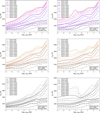 |
Fig. 2 A (top), G (middle), and M (bottom) host star results for the 3D AFGKM ExoRad GCM grid for gas giant exoplanets. We show one-dimensional (Tgas, pgas) profiles extracted from the 3D GCM models for the anti-stellar point (nightside, left) and the substellar point (dayside, right). |
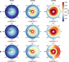 |
Fig. 3 Radial gas temperature maps of planets from the 3D AFGKM ExoRad with a global temperature, Tglobal of 800 K (left), 1600 K (center), and 2400 K (right) that orbit different host stars (top to bottom: A, G, M). The (Tgas, pgas)-maps gas are shown as equatorial slice plots. |
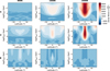 |
Fig. 4 Zonal wind speeds, U [cm/s], of planets from the 3D AFGKM ExoRad with a global average temperature of 800 K (left), 1600 K (center), and 2400 K (right) around different host stars (top to bottom: A, G, M). The values in these latitude-pressure maps are taken at the fixed longitude of the substellar point. Fig. 3 shows the equatorial (Tgas, pgas)-maps for the same models. |
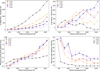 |
Fig. 5 Basic climate state diagnostics across the 3D AFGKM ExoRad for the A, F, G, K, and M host stars. Top left: differences between the day and night side averaged temperatures at pgas = 10−3 bar. Top right: differences between the morning and evening terminator temperatures, averaged over all latitudes and covering ±7.5◦ along the morning (−90◦) and evening terminator (+90◦) longitudes at pgas = 10−3 bar. Bottom left: maximum zonal mean of the zonal wind speed. Bottom right: Equatorial wind jet width in degrees latitude. |
3 Approach to accelerate exoplanet climate modelling
The approach to accelerate exoplanet climate modelling is to develop, train, and test suitable ML frameworks, and compare the ML results to ground truths in the form of deterministic GCM results, equilibrium chemistry, and transmission spectra (Fig. 6). The entire ML process starts with a dedicated study of the data representation, which utilises simulation data from the AFGKM ExoRad grid introduced in Sect. 2. We explore supervised learning techniques, including decision trees and multi-layer neural networks, to capture the underlying structure of the 3D GCM data. The practical learning of ML models is highly dependent on the volume and quality of the training data. Hence, we start by describing our data representation and necessary pre-processing details before integrating it with the ML models.
3.1 Data structure
A comprehensive study of data representation is an essential prerequisite for enhancing both training and predictive performance of ML models. The 3D AFGKM ExoRad GCM grid is used for training and testing the ML models. The grid consists of 12 planets orbiting different host stars, each with different global average temperatures Tglobal = 400 … 2600 K. These planets orbit 5 stars with different stellar types (Table A.1). Each planetary atmosphere simulation output has 42 pressure layers (pgas = 650 … 1.16 × 10⁻⁴ bar), 45 equally spaced points in latitude (θ), and 72 equally spaced points of longitude (ϕ). This data set-up defines a five-dimensional parameter space, and encompasses a total of 8 164 800 = (5 × 12 × 42 × 45 × 72) data points. For each data point, we use the information of the following quantities:
Local gas temperature: Tgas [K].
Zonal wind speed: U (east–west) [cm/s].
Meridional wind speed: V (north–south) [cm/s].
Vertical wind speed: W (up–down) [Pa/s].
For clarity in our notation, the grid refers explicitly to the 3D AFGKM ExoRad GCM grid, which encompasses the entire ensemble of 60 3D GCMs. A data point, on the other hand, is a singular point identified by five input parameters (Teff, Tglobal, pgas, θ, ϕ), each containing detailed information on four corresponding output quantities (Tgas, U, V, W). For easy identification, we refer to a specific grid planet by stellar type and global average temperature. For example, the planet orbiting the F5V star with a global average temperature of 2200 K will be referred to as F2200.
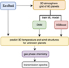 |
Fig. 6 Flowchart to derive ML-accelerated three-dimensional atmosphere models. The ML models (DNN, XGBoost) were trained to predict the gas temperature and wind structure of exoplanetary atmospheres. Step 1: a grid of pre-calculated three-dimensional planetary atmospheres (ExoRad) is used to train ML models. Step 2: the performance of the ML models is evaluated on unseen planets. Their predicted one-dimensional (Tgas, pgas)-profiles are compared to reference ground truth (Tgas, pgas)-profiles (ExoRad). Step 3: to assess how prediction errors propagate, equilibrium gas phase chemistry calculations (GGchem), performed on selected one-dimensional (Tgas, pgas)-profiles, and simulated transmission spectra (petitRADTRANS) are compared. |
3.2 Choice of machine learning models
The aim is to develop an ML model ℳη that captures a nonlinear mapping from five-dimensional input data points x ∈ ℝ5 (x = {Teff, Tglobal, pgas, θ, ϕ}) to four atmospheric output variables y ∈ ℝ4 (y = {Tgas, U, V, W}). During training, the ML model ℳη learns this mapping by minimising the error between the predicted outputs and the reference data, where η represents the trainable parameters of a model. Once trained, the model can be queried with any new data point x(q), producing a prediction ŷ(q) = ℳη(x(q)). We consider two such models: a dense neural network (DNN) denoted by  (see Fig. 8) and an Extreme Gradient Boosting (XGBoost) model denoted by
  . A key advantage of this mapping is its adaptability because all five input parameters x ∈ ℝ5 are treated as free variables, allowing ML models to predict any arbitrary combination of inputs. That implies predicting the atmospheric gas temperature profile at a specific location or extracting a particular latitudinal slice without predicting every point on a planet is possible. Furthermore, this mapping maximises the use of available data to train the ML models, allowing the models to learn something from each data point. However, a challenge arises because the number of required queries for full-planet predictions scales with the resolution of data points. For example, a complete planetary atmosphere output would require 42 × 45 × 72 = 136 080 predictions (see Sect. 3.1). ML models are inherently designed to handle such complexity by performing batch inference over large input sets. That means that increasing the number of queries has a negligible impact on computational performance, thus maintaining the practicality of the approach. In fact, for our study
  and
and  generate predictions for all atmospheric output variables across one entire planet in under two seconds on standard CPU hardware (see Sect. 6 for details).
Our ML application strategy is to systematically study and compare different ML models to find the best model for our 3D GCM dataset. We take into account the strengths and limitations of each model, such as overfitting, underfitting, training efficiency, scalability, and generalisation performance. Importantly, we evaluate these factors across a diverse range of planetary conditions, ensuring the broad applicability of the chosen model.
In addition, we explored an alternative strategy that involves four separate ML models, each dedicated to predicting a single atmospheric variable. We also investigated long short-term memory (LSTM) networks (Hochreiter & Schmidhuber 1997) as an alternative to dense architecture. However, neither the variable-specific models nor the LSTM approach yielded satisfactory performance. Therefore, this study presents results based on XGBoost and DNN trained to simultaneously predict the four atmospheric variables (Tgas, U, V, W).
3.3 Performance evaluation
Training and testing strategies: We followed a standard strategy for model development by dividing the data into 80% training and 20% validation sets. Once we achieve good prediction accuracy with the trained models, we evaluate model performance on five unseen, real planetary-like test planets (e.g., WASP-121 b*), which were not used during training or validation. Additionally, we conduct a sanity check to estimate model performance on grid-aligned test points. For this, we excluded a pair of planets (e.g., [F1800, K800]) from the training set and treated them solely for testing. While the sanity check is not strictly required, it serves as a helpful baseline to verify the predictive ability of the ML models under ideal conditions, i.e., the test data lie within the same structured parameter space as the training data.
Error analysis: We choose the root mean squared error (RMSE) and coefficient of determination (R2) (Ozer 1985; Nagelkerke et al. 1991; Di Bucchianico 2008; Chicco et al. 2021) as primary statistical metrics to evaluate the prediction accuracy of our ML models for this regression problem. Both these measures assess the differences between actual and predicted values, in our case, for all atmospheric variables corresponding to the 3D GCM data of a planet. The RMSE metric is a good indicator for comparing different models, while R2 reflects how well the prediction fits the ground truth. Mathematically R2 is defined as:  , where yi, ŷi represent the actual (observed) value of the target variable and the predicted value of the target variable obtained from the ML model, respectively.
  defines the mean of the actual target values for all data points, and n is the total number of data points. The R2 score ranges from (−∞, 1], where values closer to one reflect high prediction accuracy, which means high ML model performance, while values near zero imply that the model has limited explanatory power, leading to high prediction error. A negative R2 suggests that the ML model performs worse than a mean prediction.
We initially calculated RMSE and R2 for training and testing atmospheric variables in normalised space to assess the performance of the ML model. A high R2 value for the normalised values implies that the ML model’s prediction accuracy is good and it effectively captures most of the variance in the data. However, to capture the correct prediction accuracy, we need to transform the prediction values back from normalised to the original physical scale. It is notable that even with small prediction errors in the normalised scale, they can translate into significant deviations in the original scale, leading to higher RMSE and lower R2 values. Hence, we choose to report RMSE and R2 on the original scales to provide a more realistic measure of prediction error.
3.4 Testing unknown planets
Selection of unknown test planets: The key question in working with ML models is how useful the resulting ML predictions are in supporting the interpretation of data from current and upcoming space telescopes. Beyond validating the numerical performance of the ML models, we are particularly interested in the physical implications, specifically, whether the atmospheric chemistry derived from the ML predictions matches that of the original 3D AFGKM ExoRad GCM (Sect. 2). To explore this, five representative planets are selected from the AFGKM ExoRad GCM grid that reflect the properties of many exoplanets expected to be characterised in the coming years (Fig. 1). We explore ML models’ predictions and ExoRad differences for the PLATO target planets WASP-121 b, HATS-42 b, NGTS-17 b, WASP-23 b, and NGTS-1 b (see Sect. 5.2). We note that at least a subset of planets located in the PLATO’s LOPS2 field either have been or will be observed with other current and future telescopes to yield complementary data (Eschen et al. 2024). Among the selected planets, WASP-121 b is the best characterised so far (Davenport et al. 2025; Prinoth et al. 2025; Changeat et al. 2024, e.g.). NGTS-1 b represents the rare example of a gas giant orbiting an M dwarf star, the atmosphere of which is ideally observable with JWST. Characterising the atmospheres of such planets is an emerging research topic aimed at illuminating the planet formation process around low-mass stars (Kiefer et al. 2024; Cañas et al. 2025). The planets in the context of the grid can be seen in Fig. 7. It is important to note that it is expected that planets that lie closer to a grid planet (e.g., WASP-121 b) will perform better than planets that are further away (e.g., WASP-23 b) due to the grid structure of the training data.
Modifications: We list the planets and their respective properties selected for this study in Table 1. All grid planets have a fixed mass (0.39 Mj), a fixed radius (1 Rj) and therefore a surface gravity of 10 ms−2. The actual planets have different surface gravities: WASP-121 b (8.827 ms−2), HATS-42 b (23.82 ms−2), NGTS-17 b (12.82 ms−2), WASP-23 b (20.89 ms−2), NGTS-1 b (11.9 ms−2). For consistency with the grid simulations, we therefore assigned the same surface gravity of 10 ms−2 to all five target planets. Furthermore, as explained in Sect. 2, the calculated values for Tglobal are obtained by fixing the semi-major axis in the ExoRad simulation. Upon examining the available values, we observed minor inconsistencies between the semi-major axis and the resulting global temperatures reported in the literature. For example, for NGTS-17 b, we chose Tglobal = 1515 qK as our model input. To indicate that these planets represent modified versions of the observed systems, we denote them with an asterisk (*), for example, WASP-121 b*, throughout this study.
Prediction assessment: To evaluate ML model performance, we directly compare predictions of gas temperature and wind patterns against the corresponding outputs from the reference ExoRad GCM results. This comparison is further facilitated by analysing one-dimensional (Tgas–pgas) profiles, generating two-dimensional wind maps, and quantifying the level of agreement using R2 as our error metric.
Gas-phase chemistry: To understand the impact of the temperature deviations, we first calculate the equilibrium chemistry abundances of essential gas-phase species at the morning and evening terminators using the GGCHEM (Woitke et al. 2018) software package. We show the abundances of the following atoms and ions: H2O, CO, CO2, H, H+, CH4, NH3, HCN, SiO, TiO, MgO, FeO, SiO2, and TiO2 in Figs. 15 and 20. Substantial differences in molecules such as TiO, MgO, and SiO2 may affect cloud formation, and deviations in major gas-phase opacity sources, including CO, H2O, and TiO, may impact the observable spectrum.
Transmission spectra: To understand how strongly differences in chemical abundances could affect observations, we used petitRADTRANS (Mollière et al. 2019) to generate synthetic spectra based on both ExoRad and ML-predicted atmospheric states. We then compared the resulting spectral differences with the expected observational precision of JWST (Batalha et al. 2017), Hubble (Changeat et al. 2024), and PLATO (Grenfell et al. 2020). This allows us to evaluate whether the discrepancies may be detectable or not. We calculated the transmission spectra at the morning and evening terminators and then averaged them over each limb, as shown in Figs. 16, 21, C.5, C.4, and C.2. We have adopted the Hubble resolution from (Changeat et al. 2024), which also observed WASP-121b in this spectral range. We estimated the error for PLATO based on Grenfell et al. (2020), which discussed the feasibility of the blue and red filters. We calculated the JWST MIRI LRS and NIRSpec PRISM spectral accuracy by performing Pandexo (Batalha et al. 2017) simulations for two transits, assuming 20 pixels per bin. As with the ExoRad runs, we set the planetary mass and radius to 0.39 Mj and 1 Rj, respectively.
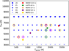 |
Fig. 7 Three-dimensional AFGKM ExoRad GCM grid of all grid planets (blue). All the randomly selected pairs of test planets removed from the training set during the sanity check (i.e., test) of ML models are highlighted with differently coloured circles for each pair, and the five target planets are put in the context of the grid. |
Test cases – selected target planets and their parameters.
4 Machine learning models
This section introduces the ML models to accelerate 3D exo-planet climate modelling and the corresponding training strategies. Our approach involves training, testing, and evaluating several ML models to determine which one is most effective with our 3D GCM data, namely, representing the 3D GCM thermodynamic structure.
4.1 Decision trees
Decision trees (DTs) are well-known ML models commonly used for classification and prediction tasks, in which training data is iteratively divided into substructures based on features to create a tree-like structure (Rokach & Maimon 2005; Kingsford & Salzberg 2008; De Ville 2013). Each tree consists of a node, a branch, and a leaf, where a node represents a decision based on a feature, a branch represents an outcome of that decision, and a leaf node represents a final prediction. The aim is to partition the data to maximise the similarity of the target variable within each subset based on criteria such as the mean squared error for the regression task. This work explores a special kind of DT model, named eXtreme Gradient Boosting (XGBoost), which is primarily based on the foundation of ensemble learning (Chen et al. 2015; Chen & Guestrin 2016). It consists of multiple shallow decision trees (called weak learners) combined sequentially to obtain a strong predictive model. The learning process in XGBoost is recursive, as a new decision tree constructed in the current state fits the residual error obtained from the tree of the previous state. That means that the current decision tree effectively corrects the prediction mistakes of the earlier trees, engaging the model in the learning process. Although XGBoost is fast to train and can provide good prediction accuracy for low-dimensional data points, it is prone to overfitting and may not generalise well to unknown test data. Therefore, this work thoroughly investigates the performance of a multi-layer neural network model as an alternative. Furthermore, we compare the performance of XGBoost and the neural network model on both training and testing datasets.
Hyperparameter optimisation: The performance of the XGBoost algorithm depends on several model parameters, such as the number of estimators, the depth of the tree structure, and others. Instead of fixing these parameters to arbitrary values to train a model, finding the best combination of parameters to obtain the model corresponding to the best choice is more effective. Finding the best set of parameters is known as hyperparameter optimisation. For our datasets, during training, we also performed hyperparameter optimisation using the ‘Random Search’ scheme to optimise the hyperparameters for the XGBoost model. For the extensive search of parameters, we define certain boundaries for each parameter (see Table 2), and the search algorithm provides the best combination of parameters by exploring this parameter space. We performed the search by fitting five folds for each of the 50 candidates, resulting in a total of 250 fits. It is essential to note that the optimal parameter sets may differ depending on the prior choice of boundaries.
Parameter space explored in XGBoost model fine-tuning.
4.2 Multi-layer neural network
To predict gas temperature and wind speeds at arbitrary query points, that is, locations not included in the training data, we employed a fully connected multi-layer dense neural network (DNN) model to encapsulate the relationship between the input parameters and atmospheric variables. We formulated the learning task as a regression problem and trained the neural network accordingly. The choice of the fully connected architecture is guided by the fact that such models are well-suited for nonlinear function approximation (i.e., as a predictor) and can capture complex nonlinear relationships with relatively low-dimensional data points (Bishop & Nasrabadi 2006; Bartlett et al. 2021). Furthermore, we aim to minimise architecture complexity by limiting the number of neurons per layer and the total number of trainable parameters. The benefit of using such architectures, defined as ‘lightweight,’ is that they reduce training time and facilitate rapid predictions, nearly in real-time. A DNN, a fundamental type of neural network architecture, comprises mainly dense layers (i.e., fully connected). The fully connected layers connect neurons from one layer to the adjacent layers, ensuring immediate and efficient information flow. A standard DNN architecture connects the input and output layers through one or more of these intermediate hidden layers (see Fig. 8). The input layer receives input parameters, which are then transformed by the hidden layers through a sequence of linear and nonlinear functions, known as forward propagation. Linear transformations are performed using weights and biases, while nonlinear transformations are defined through activation functions (Narayan 1997; Sibi et al. 2013; Sharma et al. 2017; Ramachandran et al. 2017). The activation function represents a nonlinear transformation and can take various functional forms, for example Sigmoid, rectified linear unit (ReLU), exponential linear unit (ELU), or Tanh. The output layer is necessary to predict the target variables (in our case, four atmospheric variables: local gas temperature, zonal, meridional, and vertical wind); hence, the number of neurons equals the number of output variables. We choose the mean squared error between the ground truth and predicted values as the loss function. The loss function is used to guide the correctness of the predictions by updating the weights and biases obtained through forward propagation. During the training of a neural network, the loss is initially expected to be high and will gradually decrease as the weights are fine-tuned. The learning of the neural network involves the iterative readjustment of the weights and biases of each layer through backpropagation. The updates are generally calculated using the gradient descent method via minimisation of the loss function. Although composed only of fully connected layers, such a simple yet powerful network can learn complex, nonlinear relationships, making it highly effective for regression tasks (Hornik et al. 1989; Bartlett et al. 2021).
ML model design and training strategy: Building on the objective of designing a lightweight DNN architecture, our study focuses on systematically identifying an ML model that balances predictive performance with computational efficiency in both training and inference. Initially, we start with a simple ML model (e.g. with two fully connected layers), gradually increase complexity in terms of the number of layers (up to ten) and neurons (up to 512), and obtain prediction accuracy on the test dataset for each ML model. The training of the ML models has been carried out for a maximum of 1000 training iterations (epochs), with a learning rate of 10−4, a batch size of 128, the RMSProp optimiser, and using the mean squared error as the loss function. Early stopping has been introduced and is set with a maximum of 1000 epochs, with the constraint that the training process stops if the validation loss does not improve over 25 consecutive epochs. During training, 20% of the ExoRad GCM data has been used as the validation set. Incorporating early stopping into the training of ML models helps to prevent overfitting and reduces overall training time. Among all the variations, we found that a DNN model with six fully connected (linear) layers, followed by five tanh activation (nonlinear) layers, each having 256 neurons, provides the best predictive performance while maintaining a reasonable model size, aligning with our goal of creating a lightweight yet accurate model.
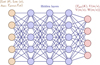 |
Fig. 8 Schematic diagram of a dense neural network that maps the five input parameters (Teff, Tglobal, pgas, Lat(θ), Lon(ϕ)) to the four output parameters (Tgas, U, V, and W) with fully connected hidden layers in between. Finally, we opted for six layers and 256 neurons each in this work. |
5 ML modelling results for an accelerated exoplanet climate modelling
This section presents the results obtained from optimised ML models (DNN, XGBoost) to predict the 3D exoplanet atmosphere gas temperature and wind structure. We adopt two complementary test approaches to thoroughly evaluate the performance of ML models. First, we remove pairs of planets from the training dataset and use them as test data. This allows us to examine the ability of the ML model to generalise unseen but on-grid planetary conditions, as presented in Sect. 5.1. Second, we evaluate the ML models using five exoplanets chosen as representatives of the LOPS2 PLATO target field in Sect. 5.2. Since these planets lie between the training grid points, this approach uniquely probes the models’ interpolation capabilities and their relevance to realistic observational scenarios. Finally, we conclude this section with an analysis of the ML-induced differences in the resulting chemical equilibrium gas compositions and transmission spectra.
5.1 Sanity check: On-grid test
We examined ML models’ prediction accuracy by removing a pair of planets (e.g., F1800 and K800) from the training set, as outlined in Sect. 3. We treated this pair as an unseen test sample and compared the ML predictions with the corresponding ExoRad outputs. We prepared five pairs of planets (F1800, K800), (G1800, K1800), (F2000, G2200), (G2000, K600), and (F400, F1600) as shown in Fig. 7 and evaluated the statistical error using RMSE and R2 metrics between the predicted and original values of atmospheric variables. We listed the resulting errors of the local gas temperature for all five planets in Table 3. We found that for DNN and XGBoost, R2 values are nearly one, indicating relatively consistent model performance across the grid. Fig. 9 displays the one-dimensional (Tgas, pgas) profiles of the pair of planets F400 and F1600 at four key locations, that is, the substellar point, the antistellar point, and the two terminators. The close agreement between the ML-predicted and actual profiles from ExoRad confirms that planet-wide high R2 value translates into equally accurate individual predicted one-dimensional profiles. The same comparison for the other planet pairs exhibits similar qualitative behaviour (see Figs. B.5–B.8), which underscores the robustness of ML predictions presented in this work.
Error metric for five pairs of randomly selected planets.
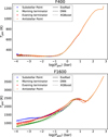 |
Fig. 9 One-dimensional (Tgas, pgas)-profiles of the two planets chosen for testing (F400, F1600). The figure shows the substellar point (blue), the antistellar point (orange), the morning terminator (green), and the evening terminator (red). The solid line shows the ExoRad simulated values, the dashed line the DNN prediction, and the dotted line the XGBoost prediction. |
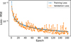 |
Fig. 10 Training and validation losses of the DNN used for predicting the test data (i.e., five target exoplanets). |
5.2 Application to PLATO exoplanet targets
In this section, we aim to demonstrate that suitably developed ML models (here: DNN, XGBoost) can reliably enrich the number of classically calculated 3D exoplanet atmosphere structures. ML-accelerated 3D model atmosphere would then enable us to conduct ensemble studies as envisioned for the PLATO targets. Therefore, we selected five inflated exoplanets that are located in PLATO’s first long pointing field, LOPS2 (Nascimbeni et al. 2025; Rauer et al. 2025). They are spread between the grid of synthetic planets used for training (Fig. 7). We evaluate the quality of the ML predictions across the training grid by comparing them to additional ExoRad models generated specifically for these planets. Sect. 5.2.2 explores whether the differences between the ML results and the ground truth (ExoRad simulations) matter in terms of chemical equilibrium abundances and observability in transmission spectra for those planets.
5.2.1 ML performance for the selected planets
As outlined earlier, it is essential to quantify the prediction accuracy of ML models. Fig. 10 shows the training and validation loss profiles during the training process of the neural network. The loss is statistically measured as the mean squared error at the end of each epoch. We calculated the loss using 80% of the training data and 20% of the validation data based on a normalised scale. To monitor the loss, we used an early stopping criterion, which was triggered after 163 epochs, with the lowest validation loss of 1.9 × 10⁻⁵ occurring at epoch 138. The training and validation loss profiles are closely aligned after 25 epochs. This indicates that the model learned effectively and generalised well, with no significant signs of overfitting. The model with minimal validation loss is saved and subsequently used to make predictions on the test data (i.e., the five target exoplanets). For the XGBoost model, hyperparameter optimisation indicated that the best performance was achieved with a subsample ratio of 1. Although we also tested the model with other values, such as 0.4, 0.6, and 0.8 (Table 2), we observed that using the full dataset (i.e., a subsample ratio of 1) in each boosting round yielded the most accurate results.
We compared the prediction accuracy of the DNN and XGBoost for the five PLATO target planets. The prediction accuracy is presented in Table 4. As expected, the DNN model consistently achieved high accuracy in temperature prediction. For all test cases, R2 scores exceeded 0.99. On the other hand, overall prediction accuracy for the horizontal wind yielded lower R2 scores. As we observed in earlier tests, the vertical wind remains the most challenging variable to predict accurately and reliably. With test planets WASP-121b* and WASP-23b*, zonal and meridional wind prediction maintained a good performance, with R2 values above 0.9. However, for the test planets NGTS-17b* and NGTS-1b*, accuracy fell significantly below this threshold. Particularly for NGTS-1b*, where the meridional wind prediction drops to 0.41. HATS-42 b* showed comparatively better results, achieving R2 values of 0.95 for zonal wind and 0.81 for meridional wind, respectively.
While XGBoost exhibited similar overall trends, a key difference from the results in Sect. 5.1 is that it was consistently outperformed by the DNN. This outcome was expected as XGBoost generally tends to excel along structured lines of the grid, whereas the DNN seems better equipped to learn the underlying physical patterns across the grid. The most striking exception occurs in the temperature prediction for NGTS-1 b*, where XGBoost achieved only R2 values of 0.7, compared to 0.99 for the DNN.
Error estimation using coefficient of determination (R2) values for PLATO target test planets.
5.2.2 Significance of the differences
We have already shown that the gas temperature predictions across all planets agree quite well numerically. Next, we examine whether and how these differences affect the numerically best and worst performing planets (Table 4). These correspond to the hottest and coolest selected planets: WASP-121 b* and NGTS-1 b*, respectively. The results for these planets are therefore representative of the whole set of selection PLATO target test planets (see also Appendix C).
WASP-121 b*: For WASP-121 b*, the DNN temperature predictions closely match the reference 3D GCM simulation, with only slight deviations appearing in the uppermost regions of the atmosphere (Fig. 11). This close agreement is also reflected in the equilibrium chemistry results (Fig. 15). The prediction from XGBoost displays a more noticeable, nearly constant offset in the one-dimensional gas temperature profiles. The constant offset and even the larger temperature difference between 101 … 102 bar do not significantly affect the chemical composition. The main difference in the gas phase composition is found for the pgas = 100 … 10−4 bar, and the effects are more prominent at the evening terminator (Fig. 15). Figs. 13 and 14 show that the exact values for zonal and meridional wind might differ in certain areas, but the trends are well captured, especially for the DNN. This visual comparison agrees with the numerical findings in the Table 4.
To ensure that the selected profiles of the substellar point, the anti-stellar point, and the two terminators are not biased selections, the absolute gas temperature difference for each point on the planet is shown in Fig. 12. Although XGBoost shows different accuracy across the range of temperatures at different pressure layers, the DNN performs more consistently throughout the atmosphere. Fig. 16 presents the transmission spectra computed with petitRADTRANS, a testament to the precision of the prediction from ML models. These transmission spectra are calculated based on equilibrium chemistry data obtained from GGchem. The second row in Fig. 16 provides a detailed comparison between the ExoRad and the ML calculated transmission spectra from the row above, with the spectral resolutions of PLATO, Hubble, JWST MIRI LRS, and JWST NIRSpec PRISM. Both predicted spectra align closely with the general shape, and all the absorption features are accurately reproduced. The DNN predictions show a slight offset on the edge of detectability between λ = 1 … 3 µm, but the deviation never exceeds 16 ppm. It is worth noting that at about 1 µm, we observe a shift from overestimation to underestimation of the features.
This trend is more pronounced in the XGBoost prediction, which exhibits the same trend but with a higher offset. In the wavelength range λ > 1 µm, the offset remains nearly constant at around 50 ppm. On the other hand, the error increases to as much as 90 ppm for λ < 1µm, with distinct differences in spectral features. When we compare the differences in chemistry in Fig. 15, it becomes evident that the almost continuous offset in the spectra is not primarily due to the difference in chemical composition. The key contributing factor is the local gas temperature difference, a significant variable that leads to differences in the atmospheric scale height ( ). This also explains the larger offset of the XGBoost prediction. As WASP-121 b is an ultra-hot Jupiter, its atmospheric scale height is so large that even relatively small temperature differences substantially impact the resulting spectrum. The increased column of absorbing material leads to an increase in the line of sight, and therefore, to this type of continuous offset.
NGTS-1 b*: After comparing the ML predicted local gas temperature for all five test planets WASP-121 b*, HAST-42b, NGTS-17 b*, WASP-23 b*, and NGTS-1 b*, against ExoRad, we can conclude that the prediction error is highest for NGTS-1 b*. While the DNN prediction shows minor differences in the atmosphere regions pgas < 10−1 bar (Figs. 22, 18 19), the XGBoost shows substantial discrepancies throughout the atmosphere.
In contrast to WASP-121 b* (see Figs. 11, 15), where the temperature offset had a limited impact on equilibrium chemistry, a persistent temperature offset leads to a significant deviation in equilibrium chemistry in the case of NGTS-1 b* (Fig. 20). The inaccurate gas temperature predictions from XGBoost cause various chemical species to differ by multiple orders of magnitude from those derived based on the ExoRad results, which are considered the ground truth in ML terms (solid vs. dotted lines). The DNN, however, maintains strong predictive performance in most of the atmosphere of NGTS-1 b*. The most noticeable differences between the DNN and the ExoRad results (solid vs dashed lines in Fig. 20 appear in the low-pressure regions (pgas < 10−1 bar), high up in the atmosphere. The problematic constituents are CO, CO2, TiO, HCN, and H. The carbon-bearing species: CO, CO2 and HCN have the largest deviation at the pgas = 10−2 bar for the DNN results. For pgas < 10−1 bar, the DNN fits almost perfectly with the ExoRad result, even for this difficult planet. The strong gas opacity sources H2O and CH4 appear to be only marginally affected. Potentially interesting species as cloud formation precursors TiO, Fe, and FeO start to differ in the regions pgas < 10−2 bar. They are very low in concentration and show an approximately constant offset. SiO and SiO2 appear not to be affected. In agreement with our earlier results in Table 4, NGTS-1 b* shows the strongest differences observed between our ML-accelerated GCM and our ExoRad GCM results. The general shape of the resulting transmission spectra in Fig. 21 is well reproduced. However, deviations of up to 100 ppm are seen in the DNN predictions, and up to 400 ppm in those from XGBoost. In the DNN predicted spectrum, all key chemical features are present, though the CO2 band at 4.5 µm and the HCN band at 15 µm are underestimated. This aligns with the reduced concentrations of CO2 and HCN compared to the ExoRad results. However, none of those differences is large enough to be observationally significant. The XGBoost prediction shows detectable errors throughout the whole spectral range. As seen in the case of WASP-121 b*, we can observe an almost constant offset due to the temperature difference. This explains why the predictions are outside the acceptable spectral accuracy for most wavelengths. Despite the substantial discrepancies shown in equilibrium chemistry (see Fig. 20), where most of the abundances differ by several orders of magnitude, the only feature missing is the CO2 at 4.5 µm. The Na and K lines have also almost completely disappeared in the XGBoost prediction. The temperature predicted by XGBoost at the morning terminator falls to ∼500 K, significantly below the expected 600–800 K for pressures pgas < 10−1 bar as shown in Fig. 22. This is the temperature regime where Na and K start to condense out of the gas phase. On the evening terminator side, temperatures hover around ∼600 K, which explains why we still get a feature at all.
A direct comparison of the spectral accuracy of WASP-121 b* and NGTS-1 b* for JWST cameras in Figs. 16 and 21 express significantly higher accuracy for the hotter planet orbiting the brighter star. This also explains why the spectra of WASP-121 b* exhibit detectable offsets despite having much smaller absolute errors than those of NGTS-1 b*. The remaining three planets exhibit similar trends, as shown in their spectra in Figs. C.5, C.4, and C.2. In contrast to the numerical results in Table 4, HATS-42 b* and NGTS-17 b* show such strong agreement across all spectral predictions that no detectable differences arise with any of the selected cameras for both ML methods. Local chemical equilibrium is a valid assumption for ultra-hot Jupiters, such as WASP-121b, and is challenging to disentangle from the effects of cloud formation (Molaverdikhani et al. 2020). Kinetic chemistry that particular effects CH4 becomes important for planets such as NGTS-1b (Bangera et al. 2025; Baeyens et al. 2021, 2022). Horizontal advection may also lead to deviations from local chemical equilibrium (Drummond et al. 2020; Baeyens et al. 2021). However, local chemical equilibrium is the ‘ground state’ even for kinetic chemistry processes. Furthermore, although the wind prediction results are less accurate, the main effects are still present, particularly the strong zonal wind jet, which is fairly reproduced.
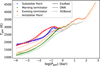 |
Fig. 11 WASP-121 b* 1D (Tgas, pgas)- profiles for the substellar (blue) and antistellar points (orange) as well as the morning (green) and evening terminators (red). The solid line is the ExoRad simulated values, the dashed line the DNN prediction, and the dotted line the XGBoost prediction. |
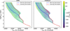 |
Fig. 12 WASP-121 b* scatter plot of the absolute gas temperature difference at each point on the planet. Overplotted are the morning (blue) and evening (red) terminator profiles as reference. |
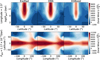 |
Fig. 13 WASP-121 b* zonal wind comparison through the atmosphere. The top row shows a latitude–pressure map at a fixed longitude of 2.5◦, which is the closest grid point to the substellar point. The bottom row shows a latitude–longitude map at the pgas = 1.17 × 10⁻³ bar. |
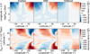 |
Fig. 14 WASP-121 b* meridional wind comparison through the atmosphere. The setup is the same as in Fig. 13. |
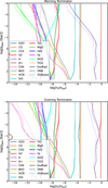 |
Fig. 15 WASP-121 b* morning (top) and evening (bottom) terminator gas phase chemistry for selected species. The solid line shows the ExoRad simulated values, the dashed line shows the DNN prediction, and the dotted line indicates the XGBoost prediction. |
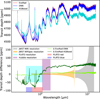 |
Fig. 16 WASP-121 b* combined morning and evening terminator transmission spectra. The first row panel shows the ExoRad, DNN, and XGBoost results. The second row shows the difference of the ML spectra to ExoRad in comparison to the spectral accuracy of JWST MIRI LRS, JWST NIRSpec PRISM, Hubble, and PLATO. |
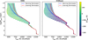 |
Fig. 17 NGTS-1 b* scatter plot of the absolute temperature difference at each point on the planet. Overplotted are the morning (blue) and evening (red) terminators as reference. |
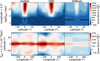 |
Fig. 18 NGTS-1 b* zonal wind comparison through the atmosphere. The top row shows a latitude-pressure map at a fixed longitude of 2.5◦, which corresponds to the closest grid point to the substellar point. The bottom row shows a latitude–longitude map at a fixed pressure level of 1.17 × 10⁻³ bar. |
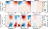 |
Fig. 19 NGTS-1 b* meridional wind comparison through the atmosphere. The setup is the same as in Fig. 18. |
6 Computational complexity
Simulating planetary atmospheres using the 3D ExoRad GCM is computationally intensive (Schneider et al. 2024). Both ExoRad and the ML models were run on the same computer system to benchmark performance. The runtime of ExoRad varies with the average global temperature Tglobal. For hot planets, Tglobal = 1400 … 2600 K, simulations take approximately 40 hours; for intermediate temperatures (1200 … 1000 K), around 60 hours; and for colder planets (800 … 400 K), runtimes can reach up to 240 hours for a 1000-planet-days simulation. These simulations utilise 64 CPU cores on a system with a AMD EPYC 7742 processor running at a base clock of 2.25 GHz. While a single GCM simulation can take anywhere from 40 to 240 hours, depending on the temperature regime, ML models significantly reduce computational time. Training the DNN with early stopping takes us approximately 25–28 hours. The XGBoost model trains even faster, taking only 15–20 minutes. For comparison, in each case, even the more time-intensive DNN training is faster than a single GCM run, while XGBoost training is orders of magnitude quicker.
Once trained, both models can generate predictions for an entire unknown planet in just a few seconds, resulting in a dramatic reduction in runtime compared to GCM simulations. For instance, a 40-hour (144 000 seconds) simulation for hot planets can be replaced with ML inference, yielding a speed-up of approximately (105). For colder planets, where GCM runtimes can reach up to 240 hours (864 000 seconds), the computational gain can reach five to nearly six orders of magnitude.
When evaluating runtime efficiency, it is crucial to distinguish between the training and inference (or testing) phases. While training, particularly for the DNN, can be time-consuming, it is also a one-time cost. This cost may increase with denser training grids, but it does not affect the prediction time for new planets. However, inference time is the correct relevant metric for practical applications, as it determines the cost of predictions for unknown planetary atmospheres. Due to their nearly real-time inference capabilities, ML models are highly effective for the rapid and scalable analysis of exoplanet atmospheres.
Instead of running computationally expensive GCM simulations for each new or unknown planet, ML models provide fast and reasonably accurate predictions, enabling efficient exploration of large parameter spaces.
XGBoost significantly reduces training time compared to a multi-layer neural network. However, this comes at a significant trade-off in prediction accuracy. We observed that increasing the density of the training grid (see Appendix B.3) improves XGBoost’s predictive performance, narrowing the accuracy gap between XGBoost and neural network models for equilibrium chemistry calculation. In such cases, XGBoost becomes a more favourable option, particularly when minimising training time is a priority without compromising too much on accuracy.
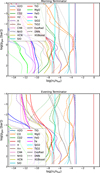 |
Fig. 20 NGTS-1 b* morning (top) and evening (bottom) terminator gas phase chemistry for selected species. The solid line shows the ExoRad simulated values, the dashed line the DNN prediction, and the dotted line the XGBoost prediction. The differences between these two terminators demonstrate how temperature asymmetries of the terminators affect the chemical gas phase composition. |
7 Summary and conclusion
We have introduced and analysed the 3D AFGKM ExoRad grid for gas giant atmospheres to study the systematic climate characteristics. We focused on solar metallicity ([Fe/H]=0) and the solar C/O ratio (0.55), which is valid as a first assumption for Jupiter mass planets (Sun et al. 2024). Higher metallicities are expected from planetary accretion models, typically for planets of Saturn mass or less (Schneider & Bitsch 2021), which are not considered in this study. Based on the analysis of four characteristic properties (day-night and morning-evening temperature differences, maximum zonal wind velocity, and wind jet width), climate states can be identified. It can be concluded that the observation of terminator temperature asymmetries is better suited to diagnose the complexity of wind jet structures on tidally locked gas giants than the canonical day-to-night side temperature differences.
This work demonstrates that, among the ML methods we tested, a lightweight DNN is the most effective at interpolating a grid of exoplanet atmospheres by predicting the local gas temperature and horizontal winds. The local gas temperature prediction is so accurate that chemical equilibrium modelling reproduces the abundances of most of the key molecules (H2O, CO, CO2, NH3, HCN) within much less than one order of magnitude compared to the ExoRad ’ground truth’. CO and CO2 are the most sensitive to temperature deviations. However, even differences in CO abundances are at most one order of magnitude, with the largest difference in the upper atmosphere (pgas < 10−1) of the coldest (NGTS-1 b*, Tglobal = 800 K) planet.
The resulting spectra show all of the main absorption features. The differences in spectra are small enough not to be detectable by PLATO, Hubble, or JWST in the three planets NGTS-1 b*, HATS-42 b*, and NGTS-17 b*. WASP-23 b* (Tglobal = 1115 K) shows single detectable features that are still smaller than 32ppm. WASP-121 b*, the hottest investigated planet, is the only one that shows a general offset of 16 ppm between 1–3 µm that could, in principle, be detectable. However, constant offsets in JWST transmission spectra of more than 100 ppm can already be generated by instrumental effects alone (Carter et al. 2024). Therefore, it is generally assumed that the transmission spectra are insensitive to uniform shifts (Rackham & de Wit 2024). Thus, even this deviation between the spectra generated with the preferred ML method (such as a lightweight multi-layer NN) and the GCM is inconsequential. We also note that different GCMs can exhibit differences in the local gas temperature of up to 200 K for the same planet (Bell et al. 2024; Coulombe et al. 2023; Noti et al. 2023). Although the horizontal wind predictions capture the global trends, the predicted values can differ in specific regions and should therefore not be interpreted as accurate at individual locations. In many cases, the wind speed deviations are smaller than 20% , and in some instances, they are smaller than the differences in wind speed obtained from other GCMs. In this work, we found deviations of up to 50% in the maximum wind velocity and, in some cases, differences in the basic wind jet structure arising from variations in numerical setups and the choice of the Navier–Stokes equations (Heng et al. 2011; Mayne et al. 2019; Noti et al. 2023). Overall, the vast majority of GCMs, including the one used in this study, exhibit qualitative agreement in their predicted wind structures for tidally locked, irradiated gas giants. The GCM we used also exhibits little time variability (by a few tens of kelvins in temperature and less than 10% in wind speed) during longer run times, once the simulations have converged, when accounting for numerical sources of instabilities (e.g. Komacek 2025; Carone et al. 2020; Schneider et al. 2022a). The stability of the GCM is also elucidated in Fig. 5 (top right), for example, where the efficacy of super-rotation shaping the evening and morning terminator temperatures can be clearly linked to orbital periods and global temperatures. In this context, the ML predictions are very well within the variations given by the underlying model framework, both for the local gas temperature and the horizontal wind velocities.
This work presents the first proof-of-concept study in which ML models are explored to directly predict the three major atmospheric variables (Tgas, U, and V). The developed neural network model is lightweight, thereby reducing memory usage during training and inference. As a result, they can predict the complete three-dimensional solution of an unknown planet within the grid space in nearly real-time. In conclusion, ML models offer a computationally efficient alternative and can serve as fast and efficient climate emulators after they are trained on a traditional GCM grid.
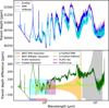 |
Fig. 21 NGTS-1 b* combined morning and evening terminator spectra. The setup is the same as in Fig. 16. |
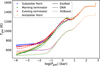 |
Fig. 22 NGTS-1 b* 1D (Tgas, pgas)-profiles for the substellar (blue) and antistellar points (orange), the morning (green) and evening terminators (red). The solid line is the ExoRad simulated values, the dashed line the DNN prediction, and the dotted line the XGBoost prediction. |
Acknowledgements
Vienna Science Cluster (VSC) HPC facility CPU time project 3D GCMs for Exoplanets (72245).
References
- Allard, N. F., Spiegelman, F., Leininger, T., & Molliere, P. 2019, A&A, 628, A120 [NASA ADS] [CrossRef] [EDP Sciences] [Google Scholar]
- Asplund, M., Grevesse, N., Sauval, A. J., & Scott, P. 2009, ARA&A, 47, 481 [CrossRef] [Google Scholar]
- Baeyens, R., Decin, L., Carone, L., et al. 2021, MNRAS, 505, 5603 [NASA ADS] [CrossRef] [Google Scholar]
- Baeyens, R., Konings, T., Venot, O., Carone, L., & Decin, L. 2022, MNRAS, 512, 4877 [NASA ADS] [CrossRef] [Google Scholar]
- Bangera, N., Helling, C., Guilluy, G., et al. 2025, ApJ, 980, 147 [Google Scholar]
- Bartlett, P. L., Montanari, A., & Rakhlin, A. 2021, Acta Numer., 30, 87 [Google Scholar]
- Batalha, N. E., Mandell, A., Pontoppidan, K., et al. 2017, Publ. Astron. Soc. Pac., 129, 064501 [Google Scholar]
- Baxter, C., Désert, J.-M., Parmentier, V., et al. 2020, A&A, 639, A36 [EDP Sciences] [Google Scholar]
- Bell, T. J., Crouzet, N., Cubillos, P. E., et al. 2024, Nat. Astron., 8, 879 [Google Scholar]
- Bishop, C. M., & Nasrabadi, N. M. 2006, Springer, 4 [Google Scholar]
- Borysow, A. 2002, A&A, 390, 779 [NASA ADS] [CrossRef] [EDP Sciences] [Google Scholar]
- Borysow, A., & Frommhold, L. 1989, ApJ, 341, 549 [NASA ADS] [CrossRef] [Google Scholar]
- Borysow, J., Frommhold, L., & Birnbaum, G. 1988, ApJ, 326, 509 [NASA ADS] [CrossRef] [Google Scholar]
- Borysow, A., Frommhold, L., & Moraldi, M. 1989, ApJ, 336, 495 [NASA ADS] [CrossRef] [Google Scholar]
- Borysow, A., Jorgensen, U. G., & Fu, Y. 2001, J. Quant. Spec. Radiat. Transf., 68, 235 [NASA ADS] [CrossRef] [Google Scholar]
- Cañas, C. I., Lustig-Yaeger, J., Tsai, S.-M., et al. 2025, arXiv e-prints [arXiv:2502.06966] [Google Scholar]
- Campos Estrada, B., Lewis, D. A., Helling, C., et al. 2025, A&A, 694, A275 [NASA ADS] [CrossRef] [EDP Sciences] [Google Scholar]
- Carone, L., Keppens, R., & Decin, L. 2015, MNRAS, 453, 2412 [Google Scholar]
- Carone, L., Baeyens, R., Mollière, P., et al. 2020, MNRAS, 496, 3582 [NASA ADS] [CrossRef] [Google Scholar]
- Carone, L., Helling, C., Gernjak, S., Leitner, H., & Janz, T. 2025, A&A, accepted [arXiv:2511.01548] [Google Scholar]
- Carter, A. L., May, E. M., Espinoza, N., et al. 2024, Nat. Astron., 8, 1008 [Google Scholar]
- Chan, Y. M., & Dalgarno, A. 1965, Proc. Phys. Soc., 85, 227 [NASA ADS] [CrossRef] [Google Scholar]
- Changeat, Q., Skinner, J. W., Cho, J. Y., et al. 2024, ApJSS, 270, 34 [Google Scholar]
- Chen, T., & Guestrin, C. 2016, in Proceedings of the 22nd ACM SIGKDD International Conference on Knowledge Discovery and Data Mining, 785 [Google Scholar]
- Chen, T., He, T., Benesty, M., et al. 2015, R package version 0.4–2, 1, 1 [Google Scholar]
- Chicco, D., Warrens, M. J., & Jurman, G. 2021, PeerJ Comput. Sci., 7, e623 [CrossRef] [Google Scholar]
- Coulombe, L.-P., Benneke, B., Challener, R., et al. 2023, Nature, 620, 292 [NASA ADS] [CrossRef] [Google Scholar]
- Cowan, N. B., & Agol, E. 2011, ApJ, 729, 54 [Google Scholar]
- Dalgarno, A., & Williams, D. A. 1962, ApJ, 136, 690 [NASA ADS] [CrossRef] [Google Scholar]
- Davenport, B., Kennedy, T., May, E., et al. 2025, AJ, 169, 260 [Google Scholar]
- De Ville, B. 2013, Wiley Interdiscip. Rev. Comput. Stat., 5, 448 [Google Scholar]
- Deline, A., Cubillos, P., Carone, L., et al. 2025, A&A, 699, A150 [NASA ADS] [CrossRef] [EDP Sciences] [Google Scholar]
- Demangeon, O. D. S., Cubillos, P. E., Singh, V., et al. 2024, A&A, 684, A27 [NASA ADS] [CrossRef] [EDP Sciences] [Google Scholar]
- Di Bucchianico, A. 2008, ESQR [Google Scholar]
- Drummond, B., Hébrard, E., Mayne, N. J., et al. 2020, A&A, 636, A68 [NASA ADS] [CrossRef] [EDP Sciences] [Google Scholar]
- Eschen, Y. N. E., Bayliss, D., Wilson, T. G., et al. 2024, MNRAS, 535, 1778 [NASA ADS] [CrossRef] [Google Scholar]
- Espinoza, N., Steinrueck, M. E., Kirk, J., et al. 2024, Nature, 632, 1017 [CrossRef] [Google Scholar]
- Goyal, J. M., Mayne, N., Drummond, B., et al. 2020, MNRAS, 498, 4680 [NASA ADS] [CrossRef] [Google Scholar]
- Gray, D. F. 2008, The Observation and Analysis of Stellar Photospheres (Cambridge, UK: Cambridge University Press) [Google Scholar]
- Grenfell, J. L., Godolt, M., Cabrera, J., et al. 2020, Exp. Astron., 50, 1 [NASA ADS] [CrossRef] [Google Scholar]
- Hammond, M., Bell, T. J., Challener, R. C., et al. 2024, AJ, 168, 4 [Google Scholar]
- Helling, C. 2021, ExoFrontiers (IOP Publishing Ltd) [Google Scholar]
- Helling, C., Lee, E., Dobbs-Dixon, I., et al. 2016, MNRAS, 460, 855 [NASA ADS] [CrossRef] [Google Scholar]
- Helling, C., Samra, D., Lewis, D., et al. 2023, A&A, 671, A122 [NASA ADS] [CrossRef] [EDP Sciences] [Google Scholar]
- Heng, K., Menou, K., & Phillipps, P. J. 2011, MNRAS, 413, 2380 [NASA ADS] [CrossRef] [Google Scholar]
- Hochreiter, S., & Schmidhuber, J. 1997, Neural Comput., 9, 1735 [CrossRef] [Google Scholar]
- Hornik, K., Stinchcombe, M., & White, H. 1989, Neural Netw., 2, 359 [NASA ADS] [CrossRef] [Google Scholar]
- Jørgensen, U. G., Amadio, F., Campos Estrada, B., et al. 2024, A&A, 690, A127 [NASA ADS] [CrossRef] [EDP Sciences] [Google Scholar]
- Kataria, T., Sing, D. K., Lewis, N. K., et al. 2016, ApJ, 821, 9 [NASA ADS] [CrossRef] [Google Scholar]
- Kennedy, T. D., Rauscher, E., Malsky, I., Roman, M. T., & Beltz, H. 2025, ApJ, 978, 82 [Google Scholar]
- Kiefer, S., Bach-Møller, N., Samra, D., et al. 2024, A&A, 692, A222 [NASA ADS] [CrossRef] [EDP Sciences] [Google Scholar]
- Kingsford, C., & Salzberg, S. L. 2008, Nat. Biotechnol., 26, 1011 [Google Scholar]
- Komacek, T. D. 2025, ApJ, 983, 7 [Google Scholar]
- Komacek, T. D., Showman, A. P., & Parmentier, V. 2019, ApJ, 881, 152 [Google Scholar]
- Komacek, T. D., Tan, X., Gao, P., & Lee, E. K. H. 2022, ApJ, 934, 79 [NASA ADS] [CrossRef] [Google Scholar]
- Lee, E., Helling, C., Dobbs-Dixon, I., & Juncher, D. 2015, A&A, 580, A12 [NASA ADS] [CrossRef] [EDP Sciences] [Google Scholar]
- Lee, E., Dobbs-Dixon, I., Helling, C., Bognar, K., & Woitke, P. 2016, A&A, 594, A48 [NASA ADS] [CrossRef] [EDP Sciences] [Google Scholar]
- Line, M. R., & Parmentier, V. 2016, ApJ, 820, 78 [Google Scholar]
- Lines, S., Mayne, N., Boutle, I. A., et al. 2018, A&A, 615, A97 [NASA ADS] [CrossRef] [EDP Sciences] [Google Scholar]
- Lissauer, J. J., Batalha, N. M., & Borucki, W. J. 2023, in Astronomical Society of the Pacific Conference Series, 534, Protostars and Planets VII, eds. S. Inutsuka, Y. Aikawa, T. Muto, K. Tomida, & M. Tamura, 839 [Google Scholar]
- Lueber, A., Kitzmann, D., Fisher, C. E., et al. 2023, ApJ, 954, 22 [NASA ADS] [CrossRef] [Google Scholar]
- Martin, P.-Y. 2019, Encyclopaedia of exoplanetary systems [Google Scholar]
- Matuszewski, F., Nettelmann, N., Cabrera, J., Börner, A., & Rauer, H. 2023, A&A, 677, A133 [NASA ADS] [CrossRef] [EDP Sciences] [Google Scholar]
- Mayne, N. J., Drummond, B., Debras, F., et al. 2019, ApJ, 871, 56 [Google Scholar]
- Molaverdikhani, K., Helling, C., Lew, B. W. P., et al. 2020, A&A, 635, A31 [NASA ADS] [CrossRef] [EDP Sciences] [Google Scholar]
- Mollière, P., Wardenier, J., Van Boekel, R., et al. 2019, A&A, 627, A67 [NASA ADS] [CrossRef] [EDP Sciences] [Google Scholar]
- Morley, C. V., Mukherjee, S., Marley, M. S., et al. 2024, ApJ, 975, 59 [NASA ADS] [CrossRef] [Google Scholar]
- Murphy, M. M., Beatty, T. G., Schlawin, E., et al. 2024, Nat. Astron., 8, 1562 [NASA ADS] [CrossRef] [Google Scholar]
- Nagelkerke, N. J. et al. 1991, Biometrika, 78, 691 [CrossRef] [Google Scholar]
- Narayan, S. 1997, Inform. Sci., 99, 69 [Google Scholar]
- Nascimbeni, V., Piotto, G., Cabrera, J., et al. 2025, A&A, 694, A313 [NASA ADS] [CrossRef] [EDP Sciences] [Google Scholar]
- Noti, P. A., Lee, E. K. H., Deitrick, R., & Hammond, M. 2023, MNRAS, 524, 3396 [NASA ADS] [CrossRef] [Google Scholar]
- Ozer, D. J. 1985, Psychol. Bull., 97, 307 [Google Scholar]
- Parmentier, V., Fortney, J. J., Showman, A. P., Morley, C., & Marley, M. S. 2016, ApJ, 828, 22 [Google Scholar]
- Patience, J., King, R. R., De Rosa, R. J., et al. 2012, A&A, 540, A85 [NASA ADS] [CrossRef] [EDP Sciences] [Google Scholar]
- Pecaut, M. J., & Mamajek, E. E. 2013, ApJS, 208, 9 [Google Scholar]
- Petrus, S., Whiteford, N., Patapis, P., et al. 2024, ApJ, 966, L11 [NASA ADS] [CrossRef] [Google Scholar]
- Prinoth, B., Seidel, J. V., Hoeijmakers, H. J., et al. 2025, A&A, 694, A284 [NASA ADS] [CrossRef] [EDP Sciences] [Google Scholar]
- Rackham, B. V., & de Wit, J. 2024, AJ, 168, 82 [Google Scholar]
- Ramachandran, P., Zoph, B., & Le, Q. V. 2017 [arXiv:1710.05941] [Google Scholar]
- Rathcke, A. D., Buchhave, L. A., de Wit, J., et al. 2025, ApJ, 979, L19 [Google Scholar]
- Rauer, H., Aerts, C., Cabrera, J., et al. 2025, Exp. Astron., 59, 26 [Google Scholar]
- Reza, A., Kubyshkina, D., Fossati, L., & Helling, C. 2025, A&A, 694, A88 [NASA ADS] [CrossRef] [EDP Sciences] [Google Scholar]
- Richard, C., Gordon, I. E., Rothman, L. S., et al. 2012, J. Quant. Spec. Radiat. Transf., 113, 1276 [NASA ADS] [CrossRef] [Google Scholar]
- Rokach, L., & Maimon, O. 2005, Data Mining and Knowledge Discovery Handbook, 165 [Google Scholar]
- Scandariato, G., Carone, L., Cubillos, P., et al. 2024, A&A, 692, A129 [NASA ADS] [CrossRef] [EDP Sciences] [Google Scholar]
- Schleich, S., Boro Saikia, S., Changeat, Q., et al. 2024, A&A, 690, A336 [NASA ADS] [CrossRef] [EDP Sciences] [Google Scholar]
- Schmidt, T. O. B., Neuhäuser, R., Briceño, C., et al. 2016, A&A, 593, A75 [NASA ADS] [CrossRef] [EDP Sciences] [Google Scholar]
- Schneider, A. D., & Bitsch, B. 2021, A&A, 654, A71 [Google Scholar]
- Schneider, A. D., Carone, L., Decin, L., Jørgensen, U. G., & Helling, C. 2022a, A&A, 666, L11 [NASA ADS] [CrossRef] [EDP Sciences] [Google Scholar]
- Schneider, A. D., Carone, L., Decin, L., et al. 2022b, A&A, 664, A56 [NASA ADS] [CrossRef] [EDP Sciences] [Google Scholar]
- Schneider, A. D., Mollière, P., Louppe, G., et al. 2024, A&A, 682, A79 [NASA ADS] [CrossRef] [EDP Sciences] [Google Scholar]
- Sharma, S., Sharma, S., & Athaiya, A. 2017, Towards Data Sci., 6, 310 [Google Scholar]
- Showman, A. P., & Polvani, L. M. 2011, ApJ, 738, 71 [Google Scholar]
- Showman, A. P., Lewis, N. K., & Fortney, J. J. 2015, ApJ, 801, 95 [NASA ADS] [CrossRef] [Google Scholar]
- Showman, A. P., Tan, X., & Parmentier, V. 2020, Space Sci. Rev., 216, 139 [Google Scholar]
- Sibi, P., Jones, S. A., & Siddarth, P. 2013, JATIT, 47, 1264 [Google Scholar]
- Sun, Q., Wang, S. X., Welbanks, L., Teske, J., & Buchner, J. 2024, AJ, 167, 167 [CrossRef] [Google Scholar]
- Tennyson, J., Yurchenko, S. N., Al-Refaie, A. F., et al. 2016, J. Mol. Spectrosc., 327, 73 [Google Scholar]
- Tennyson, J., Yurchenko, S. N., Al-Refaie, A. F., et al. 2020, J. Quant. Spec. Radiat. Transf., 255, 107228 [NASA ADS] [CrossRef] [Google Scholar]
- Thorngren, D., Gao, P., & Fortney, J. J. 2019, ApJ, 884, L6 [Google Scholar]
- von Paris, P., Gratier, P., Bordé, P., Leconte, J., & Selsis, F. 2016, A&A, 589, A52 [NASA ADS] [CrossRef] [EDP Sciences] [Google Scholar]
- Woitke, P., Helling, C., Hunter, G., et al. 2018, A&A, 614, A1 [NASA ADS] [CrossRef] [EDP Sciences] [Google Scholar]
- Yip, K. H., Changeat, Q., Al-Refaie, A., & Waldmann, I. P. 2024, ApJ, 961, 30 [Google Scholar]
- Zhang, M., Paragas, K., Bean, J. L., et al. 2024, AJ, 169, 38 [Google Scholar]
 , where
  .
.
We note that the Na and K opacities also include pressure broadening.
We note that for slow rotations, that is in particular for hotter host stars, wind jets can be broad with little horizontal wind jet gradient (Fig. 4). Thus, 10% variations in local wind speed can result in a change of the estimate of the wind jet width by ±10 degrees in latitude.
Appendix A The complete 3D AFGKM ExoRad model grid
The gas temperature maps for the complete set of sixty-three-dimensional ExoRad GCM models are provided for all host stars (AFGKM) included in this gas giant atmosphere grid. The host star parameters are shown in Table A.1. Tables A.2–A.6 summarises the planetary global parameters Tglobal [K], Tint [K], the semi-major axis a [au], and the orbital period Porb [d]. Figs. A.1 and A.2 provide the equatorial gas temperature maps. The one-dimensional stellar and anti-stellar profiles are shown in Sec. 2.2 for all planets around A, G, and M-type stars.
Stellar parameters for the 3D ExoRad GCM grid.
Planetary parameters for A-type main-sequence host stars.
Planetary parameters for F-type main-sequence host stars.
Planetary parameters for G-type main-sequence host stars.
Planetary parameters for K-type main-sequence host stars.
Planetary parameters for M-type main-sequence host stars.
21
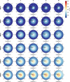 |
Fig. A.1 Radial gas temperature maps of planets from the 3D AFGKM ExoRad with global temperatures, Tglobal of 400K - 1400K (top to bottom) that orbit different host stars (left to right: A, F, G, K, M). The (Tgas, pgas)-maps gas are shown as equatorial slice plots. |
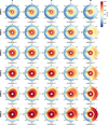 |
Fig. A.2 Radial gas temperature maps of planets from the 3D AFGKM ExoRad with global temperatures, Tglobal of 1600K - 2600K (top to bottom) that orbit different host stars (left to right: A, F, G, K, M). The (Tgas, pgas)-maps gas are shown as equatorial slice plots. |
Appendix B Supplementary results from ML testing
This section presents additional results to support the performance of ML models. Sect. B.1 provides a study of the training accuracy of our ML models. Sect. B.2 presents results from the sanity check discussed in Sect. 5.1 related to other four pairs of planets: (F1800, K800), (G1800, K1800), (F2000, G2200) and (G2000, K600). Sect. B.3 delves into enhancing the prediction quality of the XGBoost model by increasing the density of data points.
B.1 Learning efficiency of ML models
Investigating the learning capacity and efficiency of ML models is a key part of the training phase. A simple and effective way to understand learning capacity is to estimate the quality of predictions in the training data itself. The prediction error indicates whether the model is overfitting or underfitting, and this form of verification can support the selection of an appropriate model architecture. It also helps to assess the quality of training data, revealing potential issues such as sparsity (i.e., regions with low data density). Figs. B.1 and B.3 illustrate the reconstruction of the temperature using the DNN and XGBoost models, respectively, based on training data presented in Fig. 3. That means that Figs. B.1 and B.3 are the reconstructed versions of Fig. 3. Similarly, Figs. B.2 and B.4 present the reconstruction results for zonal wind slices corresponding to the input data in Fig. 4.
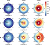 |
Fig. B.1 Re-created equatorial slice plots as in Fig. 3. The DNN has been trained on this data and is subsequently used to reproduce the same slices. |
B.2 One-dimensional profiles for pairs of test planets
This section extends the results presented in Sect. 5.1, which focused on a specific pair of planets (F400, F1600). Here, we present the prediction quality of the ML models for all sets of test planet pairs: (F1800, K800), (G1800, K1800), (F2000, G2200), and (G2000, K600). Figs. B.5 - B.8 show the predicted one-dimensional (Tgas, pgas) profiles at the substellar point, the morning terminator, the evening terminator, and the antistellar point for each of these pairs of planets.
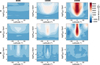 |
Fig. B.2 Zonal wind speeds from Fig. 4 reproduced by the DNN, which was trained and evaluated using the same data. |
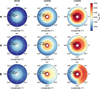 |
Fig. B.3 Re-created equatorial slice plots as in Fig. 3. The XGBoost has been trained on this data and is subsequently used to reproduce the same slices. |
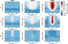 |
Fig. B.4 Zonal wind speeds from Fig. 4 reproduced by XGBoost, which was trained and evaluated using the same data. |
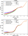 |
Fig. B.5 One-dimensional (Tgas, pgas)-profiles of the two planets chosen for test (F1800, K800). The setup is the same as in Fig. 9. |
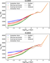 |
Fig. B.6 One-dimensional (Tgas, pgas)-profiles of the two planets chosen for test (G1800, K1800). The setup is the same as in Fig. 9. |
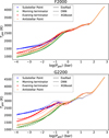 |
Fig. B.7 One-dimensional (Tgas, pgas)-profiles of the two planets chosen for test (F2000, G2200). The setup is as in Fig. 9. |
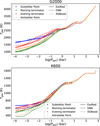 |
Fig. B.8 One-dimensional (Tgas, pgas)-profiles of the two planets chosen for test (G2000, K600). The setup is as in Fig. 9. |
B.3 Testing data density effects on XGBoost
We hypothesised that ML models, particularly XGBoost, require more data points (i.e. {Teff, Tglobal, pgas, θ, ϕ}) for improved performance. Ideally, this hypothesis should be validated using additional data points generated from the ExoRad 3D GCM model. However, producing such a dense set of points is computationally expensive, making a direct validation infeasible. To address this, we conducted a sub-optimal yet informative test by using DNN predictions as a proxy ground truth. While this approach does not provide a direct measure of accuracy against physical simulations, it effectively evaluates the sensitivity of XGBoost to increased training data point density.
We used the DNN model to predict atmospheric variables (i.e. {Tgas, U, V, W}) on sixty additional randomly selected planets within the parameter space (see green points in Fig. B.9). These new points were combined with the original training set, resulting in a denser dataset comprising 120 samples. Both the XGBoost and DNN models were retrained using this expanded dataset. Upon retraining, we observed a significant improvement in the equilibrium chemistry predictions from XGBoost (Fig. B.10). As expected, the DNN’s performance remained unchanged, as it had been retrained on data derived from its own earlier predictions, thus failing to access new features that would improve its performance. It is important to reiterate that the sole goal of this experiment is to explicitly validate the hypothesis that XGBoost could benefit from a denser sampling of the training data points, even when the additional data is obtained from another ML model rather than a physical simulation.
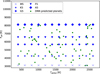 |
Fig. B.9 Scatter plot highlights the 60 randomly selected planets, shown in green. These data points and their corresponding prediction of four atmospheric variables by the DNN were integrated into the original training set. This expanded data set (120 planets in total) is utilised to evaluate the impact of increased data density on the prediction quality of the XGBoost model. |
Appendix C Supplementary results for the WASP-23, NGTS-17, and HATS-42 spectra
In Sect. 5.2.2, we show and discuss the transmission spectra for the hottest and coldest investigated test planets. The other three planets lie between those two extremes, and their simulated transmission spectra are shown in Figs. C.2, C.4 and C.5. One noticeable outlier is the spectrum for WASP-23 b*, which we discuss further here.
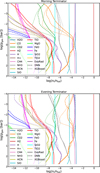 |
Fig. B.10 NGTS-1 b* morning (top) and evening (bottom) terminator gas-phase chemistry for selected species. The solid line shows the ExoRad simulated values, the dashed line the DNN prediction, and the dotted line the XGBoost prediction. The ML models are trained with 120 planets as shown in Fig. B.9. With denser data points, the prediction accuracy of the XGBoost model has improved drastically (See Fig. 20) compared to that previously trained on 60 planets. |
Transition in carbon chemistry: The global temperature of WASP-23 b* was assumed to be 1115 K. The local gas temperature thus crosses the CO - CH4 chemical conversion threshold. For hotter planets, CO is more abundant than CH4, whereas for cooler planets, CH4 is more abundant than CO, assuming equilibrium chemistry. The tendency of the XGBoost prediction to underestimate the local gas temperature (Fig. C.1) results in a situation where more CH4, and H2O, and less CO and CO2, are produced compared to ExoRad and the DNN prediction. This effect is visible in Fig. C.3. Examining the differences between the hot evening and the cold morning terminator reveals how these temperature variations impact carbon chemistry. Thus, we identified in this work two cases where the comparatively large temperature deviations of the XGBoost prediction can result in different spectral features due to critical chemical regimes. For WASP-23 b*, it is the carbon chemistry transition. For NGTS-1 b* (Fig. 21), it is the condensation that suppresses the amplitude of N and K spectral features in the XGBoost prediction.
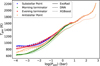 |
Fig. C.1 One-dimensional (Tgas, pgas)-profiles for the substellar (blue) and antistellar points (orange), the morning (green) and evening terminators (red) of the planet WASP-23 b*. The solid line is the ExoRad simulated values, the dashed line the DNN prediction, and the dotted line the XGBoost prediction. |
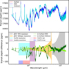 |
Fig. C.2 Combined morning and evening terminator spectra of WASP-23 b*. The setup is the same in Fig. 16. |
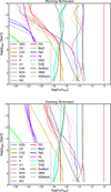 |
Fig. C.3 WASP-23 b* morning (top) and evening (bottom) terminator gas-phase chemistry for selected species. The solid line shows the ExoRad simulated values, the dashed line the DNN prediction, and the dotted line the XGBoost prediction. The differences between these two terminators demonstrate how temperature asymmetries of the terminators affect the chemical gas phase composition. |
All Tables
Error estimation using coefficient of determination (R2) values for PLATO target test planets.
All Figures
|
Fig. 1 3D ExoRad GCM grid of 60 simulated planets (blue) for different host stars from M to A (Teff [K], see Table A.1) and global planetary temperatures Tglobal [K]. Observation targets for JWST (yellow), PLATO (green), and CHEOPS (red) are overlaid. The hot Jupiters WASP-121 b, HATS-42 b, NGTS-17 b, WASP-23 b, and NGTS-1 b, highlighted in distinct colours, serve as test cases to evaluate the prediction accuracy of the ML models developed in this work. Grey points indicate objects from (Baxter et al. 2020). |
| In the text | |
|
Fig. 2 A (top), G (middle), and M (bottom) host star results for the 3D AFGKM ExoRad GCM grid for gas giant exoplanets. We show one-dimensional (Tgas, pgas) profiles extracted from the 3D GCM models for the anti-stellar point (nightside, left) and the substellar point (dayside, right). |
| In the text | |
|
Fig. 3 Radial gas temperature maps of planets from the 3D AFGKM ExoRad with a global temperature, Tglobal of 800 K (left), 1600 K (center), and 2400 K (right) that orbit different host stars (top to bottom: A, G, M). The (Tgas, pgas)-maps gas are shown as equatorial slice plots. |
| In the text | |
|
Fig. 4 Zonal wind speeds, U [cm/s], of planets from the 3D AFGKM ExoRad with a global average temperature of 800 K (left), 1600 K (center), and 2400 K (right) around different host stars (top to bottom: A, G, M). The values in these latitude-pressure maps are taken at the fixed longitude of the substellar point. Fig. 3 shows the equatorial (Tgas, pgas)-maps for the same models. |
| In the text | |
|
Fig. 5 Basic climate state diagnostics across the 3D AFGKM ExoRad for the A, F, G, K, and M host stars. Top left: differences between the day and night side averaged temperatures at pgas = 10−3 bar. Top right: differences between the morning and evening terminator temperatures, averaged over all latitudes and covering ±7.5◦ along the morning (−90◦) and evening terminator (+90◦) longitudes at pgas = 10−3 bar. Bottom left: maximum zonal mean of the zonal wind speed. Bottom right: Equatorial wind jet width in degrees latitude. |
| In the text | |
|
Fig. 6 Flowchart to derive ML-accelerated three-dimensional atmosphere models. The ML models (DNN, XGBoost) were trained to predict the gas temperature and wind structure of exoplanetary atmospheres. Step 1: a grid of pre-calculated three-dimensional planetary atmospheres (ExoRad) is used to train ML models. Step 2: the performance of the ML models is evaluated on unseen planets. Their predicted one-dimensional (Tgas, pgas)-profiles are compared to reference ground truth (Tgas, pgas)-profiles (ExoRad). Step 3: to assess how prediction errors propagate, equilibrium gas phase chemistry calculations (GGchem), performed on selected one-dimensional (Tgas, pgas)-profiles, and simulated transmission spectra (petitRADTRANS) are compared. |
| In the text | |
|
Fig. 7 Three-dimensional AFGKM ExoRad GCM grid of all grid planets (blue). All the randomly selected pairs of test planets removed from the training set during the sanity check (i.e., test) of ML models are highlighted with differently coloured circles for each pair, and the five target planets are put in the context of the grid. |
| In the text | |
|
Fig. 8 Schematic diagram of a dense neural network that maps the five input parameters (Teff, Tglobal, pgas, Lat(θ), Lon(ϕ)) to the four output parameters (Tgas, U, V, and W) with fully connected hidden layers in between. Finally, we opted for six layers and 256 neurons each in this work. |
| In the text | |
|
Fig. 9 One-dimensional (Tgas, pgas)-profiles of the two planets chosen for testing (F400, F1600). The figure shows the substellar point (blue), the antistellar point (orange), the morning terminator (green), and the evening terminator (red). The solid line shows the ExoRad simulated values, the dashed line the DNN prediction, and the dotted line the XGBoost prediction. |
| In the text | |
|
Fig. 10 Training and validation losses of the DNN used for predicting the test data (i.e., five target exoplanets). |
| In the text | |
|
Fig. 11 WASP-121 b* 1D (Tgas, pgas)- profiles for the substellar (blue) and antistellar points (orange) as well as the morning (green) and evening terminators (red). The solid line is the ExoRad simulated values, the dashed line the DNN prediction, and the dotted line the XGBoost prediction. |
| In the text | |
|
Fig. 12 WASP-121 b* scatter plot of the absolute gas temperature difference at each point on the planet. Overplotted are the morning (blue) and evening (red) terminator profiles as reference. |
| In the text | |
|
Fig. 13 WASP-121 b* zonal wind comparison through the atmosphere. The top row shows a latitude–pressure map at a fixed longitude of 2.5◦, which is the closest grid point to the substellar point. The bottom row shows a latitude–longitude map at the pgas = 1.17 × 10⁻³ bar. |
| In the text | |
|
Fig. 14 WASP-121 b* meridional wind comparison through the atmosphere. The setup is the same as in Fig. 13. |
| In the text | |
|
Fig. 15 WASP-121 b* morning (top) and evening (bottom) terminator gas phase chemistry for selected species. The solid line shows the ExoRad simulated values, the dashed line shows the DNN prediction, and the dotted line indicates the XGBoost prediction. |
| In the text | |
|
Fig. 16 WASP-121 b* combined morning and evening terminator transmission spectra. The first row panel shows the ExoRad, DNN, and XGBoost results. The second row shows the difference of the ML spectra to ExoRad in comparison to the spectral accuracy of JWST MIRI LRS, JWST NIRSpec PRISM, Hubble, and PLATO. |
| In the text | |
|
Fig. 17 NGTS-1 b* scatter plot of the absolute temperature difference at each point on the planet. Overplotted are the morning (blue) and evening (red) terminators as reference. |
| In the text | |
|
Fig. 18 NGTS-1 b* zonal wind comparison through the atmosphere. The top row shows a latitude-pressure map at a fixed longitude of 2.5◦, which corresponds to the closest grid point to the substellar point. The bottom row shows a latitude–longitude map at a fixed pressure level of 1.17 × 10⁻³ bar. |
| In the text | |
|
Fig. 19 NGTS-1 b* meridional wind comparison through the atmosphere. The setup is the same as in Fig. 18. |
| In the text | |
|
Fig. 20 NGTS-1 b* morning (top) and evening (bottom) terminator gas phase chemistry for selected species. The solid line shows the ExoRad simulated values, the dashed line the DNN prediction, and the dotted line the XGBoost prediction. The differences between these two terminators demonstrate how temperature asymmetries of the terminators affect the chemical gas phase composition. |
| In the text | |
|
Fig. 21 NGTS-1 b* combined morning and evening terminator spectra. The setup is the same as in Fig. 16. |
| In the text | |
|
Fig. 22 NGTS-1 b* 1D (Tgas, pgas)-profiles for the substellar (blue) and antistellar points (orange), the morning (green) and evening terminators (red). The solid line is the ExoRad simulated values, the dashed line the DNN prediction, and the dotted line the XGBoost prediction. |
| In the text | |
|
Fig. A.1 Radial gas temperature maps of planets from the 3D AFGKM ExoRad with global temperatures, Tglobal of 400K - 1400K (top to bottom) that orbit different host stars (left to right: A, F, G, K, M). The (Tgas, pgas)-maps gas are shown as equatorial slice plots. |
| In the text | |
|
Fig. A.2 Radial gas temperature maps of planets from the 3D AFGKM ExoRad with global temperatures, Tglobal of 1600K - 2600K (top to bottom) that orbit different host stars (left to right: A, F, G, K, M). The (Tgas, pgas)-maps gas are shown as equatorial slice plots. |
| In the text | |
|
Fig. B.1 Re-created equatorial slice plots as in Fig. 3. The DNN has been trained on this data and is subsequently used to reproduce the same slices. |
| In the text | |
|
Fig. B.2 Zonal wind speeds from Fig. 4 reproduced by the DNN, which was trained and evaluated using the same data. |
| In the text | |
|
Fig. B.3 Re-created equatorial slice plots as in Fig. 3. The XGBoost has been trained on this data and is subsequently used to reproduce the same slices. |
| In the text | |
|
Fig. B.4 Zonal wind speeds from Fig. 4 reproduced by XGBoost, which was trained and evaluated using the same data. |
| In the text | |
|
Fig. B.5 One-dimensional (Tgas, pgas)-profiles of the two planets chosen for test (F1800, K800). The setup is the same as in Fig. 9. |
| In the text | |
|
Fig. B.6 One-dimensional (Tgas, pgas)-profiles of the two planets chosen for test (G1800, K1800). The setup is the same as in Fig. 9. |
| In the text | |
|
Fig. B.7 One-dimensional (Tgas, pgas)-profiles of the two planets chosen for test (F2000, G2200). The setup is as in Fig. 9. |
| In the text | |
|
Fig. B.8 One-dimensional (Tgas, pgas)-profiles of the two planets chosen for test (G2000, K600). The setup is as in Fig. 9. |
| In the text | |
|
Fig. B.9 Scatter plot highlights the 60 randomly selected planets, shown in green. These data points and their corresponding prediction of four atmospheric variables by the DNN were integrated into the original training set. This expanded data set (120 planets in total) is utilised to evaluate the impact of increased data density on the prediction quality of the XGBoost model. |
| In the text | |
|
Fig. B.10 NGTS-1 b* morning (top) and evening (bottom) terminator gas-phase chemistry for selected species. The solid line shows the ExoRad simulated values, the dashed line the DNN prediction, and the dotted line the XGBoost prediction. The ML models are trained with 120 planets as shown in Fig. B.9. With denser data points, the prediction accuracy of the XGBoost model has improved drastically (See Fig. 20) compared to that previously trained on 60 planets. |
| In the text | |
|
Fig. C.1 One-dimensional (Tgas, pgas)-profiles for the substellar (blue) and antistellar points (orange), the morning (green) and evening terminators (red) of the planet WASP-23 b*. The solid line is the ExoRad simulated values, the dashed line the DNN prediction, and the dotted line the XGBoost prediction. |
| In the text | |
|
Fig. C.2 Combined morning and evening terminator spectra of WASP-23 b*. The setup is the same in Fig. 16. |
| In the text | |
|
Fig. C.3 WASP-23 b* morning (top) and evening (bottom) terminator gas-phase chemistry for selected species. The solid line shows the ExoRad simulated values, the dashed line the DNN prediction, and the dotted line the XGBoost prediction. The differences between these two terminators demonstrate how temperature asymmetries of the terminators affect the chemical gas phase composition. |
| In the text | |
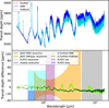 |
Fig. C.4 Combined morning and evening terminator spectra of NGTS-17 b*. The setup is as in Fig. 16. |
| In the text | |
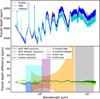 |
Fig. C.5 Combined morning and evening terminator spectra of HATS-42 b*. The setup is as in Fig. 16. |
| In the text | |
Current usage metrics show cumulative count of Article Views (full-text article views including HTML views, PDF and ePub downloads, according to the available data) and Abstracts Views on Vision4Press platform.
Data correspond to usage on the plateform after 2015. The current usage metrics is available 48-96 hours after online publication and is updated daily on week days.
Initial download of the metrics may take a while.