| Issue |
A&A
Volume 706, February 2026
|
|
|---|---|---|
| Article Number | A190 | |
| Number of page(s) | 13 | |
| Section | The Sun and the Heliosphere | |
| DOI | https://doi.org/10.1051/0004-6361/202555677 | |
| Published online | 09 February 2026 | |
Chromospheric evaporation as the driver of helium enrichment in active region solar wind: A case study
1
Shandong Key Laboratory of Optical Astronomy and Solar-Terrestrial Environment, Institute of Space Sciences, 180 Wenhua Xilu Weihai 264209 Shandong, China
2
Korea Astronomy and Space Science Institute 34055 Daejeon, Republic of Korea
3
Max Planck Institute for Solar system Research Justus-von-Liebig-Weg 3 D-37077 Gottingen, Germany
4
Space Research and Technology Institute, Bulgarian Academy of Sciences, Acad. G. Bonchev Str. Bl. 1 1113 Sofia, Bulgaria
★ Corresponding author: This email address is being protected from spambots. You need JavaScript enabled to view it.
Received:
27
May
2025
Accepted:
19
December
2025
Abstract
Context. The physical mechanisms of helium abundance (AHe) depletion in the corona and solar wind are closely linked to coronal heating, solar wind origin, and acceleration processes. The relationships between the AHe in the solar wind and the properties and activity of the source regions are crucial for understanding the depletion of AHe.
Aims. We aim to investigate the impact of active region (AR) activity and properties on the AHe in the solar wind.
Methods. First, we established the link between carefully selected ARs and the solar wind. Then, the AR chromospheric activity was quantitatively investigated using observations from the Atmospheric Imaging Assembly and Helioseismic Magnetic Imager on board the Solar Dynamics Observatory. The AR temperatures were derived with the differential emission measure method. We also statistically analyzed the AHe in the solar wind with higher and lower charge states during solar cycles 23 and 24. The parameters of solar wind were measured by the instruments on board ACE and Wind.
Results. We find that an AR with greater chromospheric activity has higher AHe in its associated solar wind. The statistical analysis shows that the median AHe in solar wind with higher charge states is higher than AHe in solar wind with lower charge states.
Conclusions. We conclude that chromospheric activity, primarily chromospheric evaporation processes, is possibly the main heating and transportation mechanism leading to a higher AHe in the corona and solar wind. This could also reasonably explain the variation in AHe in AR solar wind during different solar activity phases and the higher AHe in AR solar wind compared to quiet Sun solar wind.
Key words: Sun: abundances / Sun: activity / Sun: chromosphere / solar wind
© The Authors 2026
 Open Access article, published by EDP Sciences, under the terms of the Creative Commons Attribution License (https://creativecommons.org/licenses/by/4.0), which permits unrestricted use, distribution, and reproduction in any medium, provided the original work is properly cited.
This article is published in open access under the Subscribe to Open model. This email address is being protected from spambots. You need JavaScript enabled to view it. to support open access publication.
1. Introduction
The depletion of the helium abundance (AHe) in the corona and solar wind is closely linked to coronal heating, solar wind origin, and acceleration processes. Previous studies show that AHe in the photosphere is about 8.5% (Grevesse & Sauval 1998; Asplund et al. 2009). In both the corona and solar wind, AHe decreases relative to its value in the photosphere (Feldman 1992; von Steiger & Schwadron 2000). However, the physical mechanisms of AHe depletion in the solar wind remain unclear.
Significant differences exist in the solar wind AHe from various sources and at different speeds. AHe in the solar wind is typically below 5%, and it varies with solar activity cycles (Ogilvie & Hirshberg 1974; Feldman et al. 1978). In fast solar wind, the AHe is higher, at approximately 4%–6%, with a narrower distribution range and hardly any variance with solar cycles. In contrast, the slow solar wind has lower AHe, at approximately 1%–5%, with a broader distribution range and a stronger correlation with the solar cycles (Aellig et al. 2001; Kasper et al. 2007, 2012; Alterman & Kasper 2019; Alterman et al. 2021, 2025b). AHe in the slow solar wind is more strongly positively correlated with solar sunspot numbers than in the fast solar wind (Kasper et al. 2007, 2012; McIntosh et al. 2011). Fu et al. (2018) analyzed the statistical characteristics of AHe in solar wind from coronal holes (CHs), active regions (ARs), and quiet Sun (QS) regions. They found that CH wind has a higher AHe with a narrower distribution range, while AR and QS wind have a lower AHe with a wider distribution. Shi et al. (2024) conducted a statistical analysis of solar wind properties from CH, AR, and QS throughout solar cycles 23 and 24. Their findings showed that AHe in all three types of solar wind decreases as solar activity weakens. These studies suggest that AHe in the solar wind may be influenced by the properties and activity of the source regions.
The depletion of AHe in the corona and solar wind should be connected to the properties and activities of the chromosphere. It is generally believed that the depletion of AHe and enrichment of low first ionization potential (FIP) elements results from a more efficient process of transporting charged ions as plasma moves from the lower to the upper atmosphere and solar wind (Basu & Antia 2008). Low-FIP elements, such as Fe, Mg, and Si, ionize at lower altitudes and temperatures. That is the reason for the enrichment of low-FIP elements in the corona and solar wind (Feldman & Widing 2003). In contrast, helium is the last element to be ionized in the upper chromosphere (Del Zanna et al. 2020). Therefore, to study the causes of AHe variations in the corona and solar wind, we should investigate chromospheric activity and the properties of phenomena occurring at chromospheric heights.
Chromospheric activity, which encompasses various scales (spatial, temporal, and energetic), is a key driver of energetic coronal activity in the solar atmosphere. Microflares (Battaglia et al. 2024) and flares (Fletcher et al. 2011) are the source of the most intense such activity. The same physical processes drive both large flares and microflares (Saqri et al. 2024), albeit at different scales. Microflares are events releasing energies on the order of around 1027 erg, about six orders of magnitude less than the largest solar flares, 1033 erg (Hannah et al. 2011). The occurrence frequency of microflares is significantly higher than that of large flares. Microflares are often observed in plages (Li & Wang 1998) or within sunspots (Battaglia et al. 2024). Small-scale dynamic energetic events often occur repeatedly in ARs. These events are known as explosive events (EEs) and jet-like events. EEs are characterized by non-Gaussian spectral line profiles, which result from high-energy deposition. Similarly, jet-like events correspond to collimated plasma flows in the chromosphere and transition region. Both types of events are associated with microflares (Huang et al. 2014; Gupta & Tripathi 2015; Madjarska et al. 2022). They produce imprints in the form of intense small-scale brightenings in the chromosphere of ARs. These brightenings are the observational signature of microflare ribbons (Shibata et al. 2007; Dumin & Somov 2020). Chromospheric brightenings associated with EEs are generally located in regions with weak and mixed magnetic polarities (Chae et al. 1998). They are related to magnetic flux cancellation (Huang et al. 2014) and are believed to result from magnetic reconnection (Dere 1994; Madjarska et al. 2022). Jet-like events are related to magnetic flux convergence and cancellation, or the interaction between emerging and pre-existing flux, and are also driven by magnetic reconnection in the upper atmosphere (Raouafi et al. 2016; Shen 2021). The frequency and intensity of chromospheric activity are influenced by variations in the magnetic network. The magnetic network is a magnetic structure in the lower atmosphere driven by the convection of supergranulation, and is a concentrated distribution region of small-scale magnetic fields in the photosphere. This magnetic field can drive chromospheric jets and eruptions through shearing, reconnection, and other activities, and provide energy for these events. McIntosh et al. (2011) suggested that the state of the magnetic network is closely related to the generation of the solar wind and affects its composition and dynamical properties. During solar minimum, the weakening of magnetic activity reduces the emissivity associated with the magnetic network. The reduction of AHe during solar minima is primarily driven by changes in the heating flux from the corona to the transition region as solar activity evolves, i.e., changes in the amount of energy available to the plasma at transition-region heights. This process is closely coupled to the local magnetic network. This leads to a decrease in the intensity and frequency of chromospheric activity, resulting in insufficient heating of the fast solar wind. Spicules are continuous, small-scale, high-frequency activities in the chromosphere rooted in the magnetic network. McIntosh (2012) suggested that chromospheric spicules and their coronal counterparts contribute to the heating and acceleration of the fast solar wind.
Flares produce large areas of chromosphere brightenings known as flare ribbons (Masson et al. 2009; Fletcher et al. 2011; Tian et al. 2015). Flare ribbons are bright in Hα and UV (for example 1600 Å) emission features. They occur in the upper chromosphere and transition region. The particles accelerated by magnetic reconnection deposit their energy in these atmospheric regions, resulting in the enhanced emission observed in the flare ribbons (Graham & Cauzzi 2015; Priest & Longcope 2017). The flare ribbons are associated with the footpoints of flux tubes that newly reconnect in the flare arcade.
Flares or microflares are accompanied by so-called chromospheric evaporation (Chifor et al. 2008; Hannah et al. 2011; Tian et al. 2015). During solar flares, as was mentioned above, high-energy electrons accelerated by magnetic reconnection move downward along magnetic field lines into the lower atmosphere. This process heats the chromospheric plasma to high temperatures, observable in the soft X-ray range (Benz 2017). The overpressure from chromospheric heating drives the heated plasma upward along magnetic loops, eventually reaching the corona. This phenomenon is known as chromospheric evaporation (Hirayama 1974; Antonucci et al. 1984; Fisher et al. 1985; Veronig et al. 2002; Tian et al. 2015). Chromospheric evaporation can be categorized into two types: explosive (Milligan et al. 2006a) and gentle (Milligan et al. 2006b). The difference between the two types is the velocity at which the chromospheric material, once heated, expands into the corona (Battaglia et al. 2024).
Fu et al. (2020) found that AHe in coronal mass ejections (CMEs) is strongly related to the chromospheric evaporation process in the source regions. They classified the plasma in CMEs into three types based on their origin and generation mechanisms. The first type is directly from the corona, corresponding to plasma with low average charge states of iron (QFe) and low AHe. The second type refers to the coronal plasma heated by magnetic reconnection during flare events, which shows high QFe and relatively low AHe. The third type consists of plasma with both high QFe and high AHe, which is generated by the chromospheric evaporation. The origin and generation mechanisms and plasma characteristics of the three types of plasma in CMEs are summarized in Table 1. Subsequently, Zhai et al. (2022) classified CMEs based on whether they were accompanied by flares and hot channels. Their statistical results indicated that more than half of the hot plasma inside interplanetary CMEs (ICMEs) was heated by chromospheric evaporation before and/or during the flare event. Yogesh et al. (2022) found that both chromospheric evaporation and gravity settling together account for more than 8% of the AHe enhancement and variation in ICMEs. Furthermore, as the flare intensity increases, the proportion of material originating from chromospheric evaporation (with high AHe and QFe) in CMEs increases significantly. Meanwhile, the proportion of reconnection-heated coronal plasma remains unchanged, and the plasma directly from the corona decreases significantly (Fu et al. 2023). These studies suggest that the increase of AHe in CMEs is strongly linked to chromospheric evaporation processes.
Three types of plasma in CMEs.
The present article aims to search for answers to several fundamental questions: how the AHe and its evolution in AR solar wind are related to the characteristics and activity of the source regions, and more specifically why the distribution range of AHe in the AR solar wind is so wide, and why the AHe in the slow solar wind varies with the solar cycles. In the present study, the properties and activities of two ARs and their associated solar wind are analyzed, and the statistical properties of AHe and QFe in AR solar wind during solar cycles 23 and 24 are reported and discussed. We aim to investigate the causes of the variations of AHe in slow solar wind and identify which activity or phenomena in ARs may lead to a variation of AHe. The paper is organized as follows. In Section 2, we describe the instruments and data analysis method. The results are presented in Section 3. The discussion of the results is in Section 4. Finally, the conclusions are summarized in Section 5.
2. Data and analysis methods
In the present study, the remote sensing data of two ARs are from the Atmospheric Imaging Assembly (AIA; Lemen et al. 2012) and the Helioseismic and Magnetic Imager (HMI; Schou et al. 2012) aboard the Solar Dynamics Observatory (SDO; Pesnell et al. 2012). The AIA observes images of the solar atmosphere in seven extreme ultraviolet (EUV) and three ultraviolet (UV) wavelengths, with temperatures ranging from 6 × 10⁴ K to 2 × 10⁷ K. The spatial resolution of the EUV and UV channels was 0.6″ per pixel, with time resolutions of 12 s and 24 s, respectively. The AIA 1600 Å data are used to study the chromospheric activity in ARs. The HMI provides measurements of the photosphere magnetic field with a spatial resolution of 0.5″ per pixel and a temporal resolution of 45 s. The AR temperatures were derived with the differential emission measure (DEM) method developed by Cheung et al. (2015) and Su et al. (2018).
The in situ solar wind parameters analyzed in the present study were obtained from the Advanced Composition Explorer (ACE; Stone et al. 1998) and Wind (Steinberg et al. 1996) spacecraft. The charge states were measured by the Solar Wind Ion Composition Spectrometer (SWICS; Gloeckler et al. 1998) on board ACE. The solar wind velocity and AHe were provided by the Solar Wind Experiment (SWE; Ogilvie et al. 1995), while the interplanetary magnetic field was measured by the Magnetic Field Investigation (MFI; Lepping et al. 1995), both instruments aboard Wind. The AHe, expressed as a percentage, was calculated as the ratio of helium ion number density to proton number density. The data used for AHe calculations are available from NASA CDAWeb under the dataset WI_H1_SWE (DOI: 10.48322/NASD-J276). We used solar wind data for all parameters available from Wind, such as the solar wind velocity, magnetic field, and helium abundance. For parameters not measured by Wind, such as charge states, we used data from the ACE spacecraft.
To quantify the chromospheric activity in ARs, we adopted a measure for estimating the brightening areas that reflect this activity, which we name a proportion of brightening area (hereafter referred to as PBA). As was mentioned above, active chromospheric areas in ARs tend to exhibit frequent and intense brightenings, which are caused by chromospheric evaporation driven by magnetic reconnection in the upper atmosphere. The PBA defines the chromospheric activity level of an AR by calculating the ratio of the brightening area (for example the region outlined by the solid red line in panel (d) of Fig. 1) to the whole AR (for example the region outlined by the solid blue line in the same panel). The total areas of ARs are defined based on their associated photospheric magnetic field. The area of the entire AR corresponds to the strong magnetic-field concentration areas (MCAs) in the photosphere. To make this definition more objective, we used Br (the absolute value of the radial component of the photospheric magnetic field) to contour the MCAs, as was detailed in Fu et al. (2015).
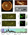 |
Fig. 1. Remote sensing properties of AR 12671. Panel (a) displays the AIA 193 Å full-disk coronal image. The green box corresponds to the position of AR 12671. Panel (b) shows the AIA 193 Å coronal map of AR 12671. Panel (c) displays the photospheric magnetic field map of AR 12671, with the solid blue line outlining the MCA. Panel (d) shows the AIA 1600 Å image corresponding to the C 7.0 flare that occurred at 21:45 UT on August 19, 2017. Panel (f) shows a small-scale chromospheric brightening event that occurred at 18:40 UT on August 19, 2017. The brightening regions are outlined by the solid red line. Panel (e) shows the 2.5–4.5 MK EM of the area outlined with a white box in Panel (d), with the orange line contouring the brightening regions. Panel (h) displays the evolution curve of the PBA over time. The vertical axis represents the ratio value of brightening areas and the whole AR ×1000. The three days of AR 12671 at the center of the solar disk are highlighted with purple, blue, and green shades, respectively. Vertical red lines (&#Xtextcircled;1–&#Xtextcircled;5) mark the time of five GOSE flares. The vertical blue line marks the time of small-scale chromospheric brightening. We can see that AR 12671 exhibited significant chromospheric activity during its time at the solar disk center. |
The chromospheric brightening areas were obtained from the AIA 1600 Å intensity images. We defined the region with intensity exceeding a certain intensity threshold as the chromospheric brightening region. The intensity threshold was defined as follows. First, the histograms of intensity distribution in MCAs were obtained (see Appendix A). Then, the intensity corresponding to the most pixels was chosen as the intensity reference value. We tested 3.5, 4.5, and 5.5 times the reference value as intensity thresholds, respectively. It was found that there is little difference in the area of the outlined brightening areas. The intensity threshold (4.5 times the reference value) was determined through testing, ensuring that most of the chromospheric brightenings were captured while minimizing background noise. A higher PBA value indicates that the brightening events are stronger. A more frequent appearance of high PBAs over time suggests that the strong brightening events are happening more frequently. Thus, PBAs can reflect the intensity and frequency of activity in the chromosphere.
To investigate the impact of chromospheric activity and properties on the AHe in the solar wind, it is crucial to link AR to the solar wind reliably. Ma et al. (2022) developed a method of linking ARs with the solar wind with high confidence. We used their method to identify the solar wind coming from ARs. The steps for linking ARs and the associated solar wind are summarized briefly below: 1. The time delay between remote observation and in situ detection was considered. It takes about four days for slow solar wind (350–450 km s−1) to travel from the Sun to the Earth. Therefore, the solar wind originating from an AR should arrive at the Earth after 3–5 days when an AR is directly facing the Earth. 2. The solar wind properties were examined. If the O7+/O6+ detected by ACE increased significantly, it was inferred that the solar wind may originate from this AR. We defined “significant high” as twice the minimum background solar wind. 3. The method compared the large-scale structure of the corona with the sequences of the in situ detected solar wind properties. 4. The radial magnetic field directions of the solar wind associated with the AR were compared with the HMI magnetic field polarities to determine from which polarity of the AR the solar wind originates.
We applied the above method to associate AR 12671 with the solar wind as an example. AR 12671 was at the center of the solar disk on day-of-year (DOY) 231 (August 19, 2017), as is shown in Fig. 1. Firstly, considering the time delay between remote and in situ observation, the solar wind associated with AR 12761 should be detected on DOY 235. Figure. 3 panel (c1) shows a significant increase in the O7+/O6+ ratio and a noticeable decrease in the solar wind speed between DOY 235 and DOY 243. Secondly, a positive-polarity CH lies to the west of AR 12671, while AR 12672 is located to the east of it. Another positive-polarity CH is located further east of AR 12672. By comparing the large-scale coronal structure with the solar wind sequence, we observe that the slow solar wind is positioned between two fast solar wind streams (Fig. 3(a1)). The sequence of the solar wind is consistent with the large-scale coronal structure. Therefore, the solar wind from DOY 235 to DOY 243 likely originated from the two ARs. AR 12672 reached the solar disk center on DOY 237 (August 25, 2017, at 20:00 UT). The solar wind associated with AR 12672 should be detected on DOY 241. The slow solar wind before DOY 241 should be associated solely with AR 12671. Thirdly, the magnetic field direction is from negative to positive polarity from DOY 235 to DOY 241. This is consistent with the HMI magnetic field data (see Fig. 1 panel (c)). The negative polarity on the west side of AR 12671 first passed through the solar disk center. Thus, the solar wind from DOY 235 to DOY 240 should originate from AR 12671. In addition, according to the Richardson and Cane1 CME list, a CME was detected near the Earth between 04:00 UT on DOY 234 (August 22, 2017) and 18:00 UT on DOY 235 (August 23, 2017). To distinguish the CME from the solar wind more clearly, we provide an approximately 12-hour gap between the solar wind from AR 12671 and the CME. This means that the solar wind detected from 06:00 UT on DOY 236 (August 24, 2017) to 23:59 UT on DOY 240 (August 28, 2017) is regarded as coming from AR 12671. The duration of the CME is indicated by blue shading in Fig. 3, top panel. The above method was also used to establish the connection between AR 12733 and its related solar wind.
3. Results
The remote sensing properties of the two ARs were first compared, followed by a comparison of the in situ solar wind properties. Notably, we identified only two typical ARs for comparison. There are three main reasons for our limited choice. First, to reliably correlate ARs with the solar wind, we required the solar disk to be relatively clear, with only the target AR present. Such ARs are typically observed during solar minimum, as during this period fewer ARs emerge. Second, we needed to identify ARs with high chromospheric activity during solar minimum. However, ARs with high activity may be accompanied by a CME. Our research primarily focuses on the steady-state solar wind, so CME interference should be excluded. Third, although more such isolated AR were found, the backmapping to the source regions was unreliable, and therefore these cases were excluded. Given these stringent conditions, we identified only two ARs suitable for comparison, to investigate the impact of chromospheric activity and properties on the AHe in the solar wind.
3.1. Comparison of chromospheric activities and properties between AR 12671 and AR 12733
The remote sensing properties and chromospheric activity of AR 12671 are shown in Fig. 1. The west limb of AR 12671 directly faced the Earth at about 18:30 UT on August 19, 2017 (DOY 231), and the east limb faced the Earth at around 23:59 UT on August 21, 2017 (DOY 233). Panel (a) shows the position of AR 12671 on the solar disk at 18:40 UT on August 19, 2017. AR 12671 has five sunspots. Its photospheric magnetic field is complex, as is shown in panel (c) of Fig. 1. The Geostationary Operational Environmental Satellite (GOES; Garcia 1994) detected five C-class flares (C 7.0, C 1.8, C 2.9, C 1.5, C 1.5) in this AR while crossing the solar disk center. GOES is composed of a series of satellites. The flare numbers and flare classes we used are provided by the GOES-14 satellite. Soft X-ray intensity peaks occurred at the following times: 21:55 UT on August 19; 04:40 UT, 07:50 UT on August 20; and 20:22 UT, 22:37 UT on August 21, indicating that high-temperature plasma was detected during all five flares. Panel (d) of Fig. 1 demonstrated the chromospheric response to the C 7.0 flare, with strong flare ribbons caused by the flare occurrence.
We performed a DEM analysis using the AIA/SDO data on the area outlined in the white box in Panel (d). Panel (e) presents the 2.5–4.5 MK emission measure (EM) for the C 7.0 flare. The temperatures of the flare ribbon plasma reach up to 20 MK (for more details see Appendix B). Additionally, numerous small-scale chromospheric brightening events were observed while AR 12671 was facing the Earth. Panel (f) shows an example of one small-scale brightening. Panel (g) of Fig. 1 shows the 5–8 MK EM for the small-scale chromospheric brightening. Higher-temperature plasma was also detected during this brightening (see Appendix B). These results suggest that frequent small-scale chromospheric brightening events are also accompanied by high-temperature plasma at temperatures of a few million Kelvin.
Panel (h) shows the PBA that indicates the chromospheric activity during the AR 12671 across the solar disk center. The black curve represents the temporal evolution of the PBA for two regions: the brightening area (outlined by the solid red line) in the AIA 1600 Å image and the MCA (outlined by the solid blue line). A higher ratio indicates greater chromospheric activity. The vertical red lines (&#Xtextcircled;1–&#Xtextcircled;5) in panel (h) mark the occurrence time of the five C-class flares. The vertical blue line next to &#Xtextcircled;1 marks the moment when the small-scale chromospheric brightening shown in panel (f) occurred. During the flares, the brightening ratios increased significantly, with the PBA higher than 10‰. During AR 12671 located at the center of the solar disk, the PBA exceeds 2‰ (5‰) for 32% (10%) of the period. In particular, on August 20 (marked by the blue-shaded area), the PBA exceeded 2‰ (5‰) for nearly two thirds (half) of the day. These results indicate that AR 12671 has frequent and strong chromospheric activity.
The remote sensing properties and chromospheric activity of AR 12733 are shown in Fig. 2. The AR crossed the solar disk center from 20:00 UT on January 23, 2019, to 23:59 UT on January 24, 2019. Panel (a) displays the position of AR 12733 on the solar disk at 13:40 UT on January 24, 2019. As is shown in panel (b) of Fig. 2, AR 12733 has a simple photospheric magnetic field structure. It is a typical bipolar sunspot AR. GOES detected no flares during this period. Occasional small point-like brightening was observed in the AIA 600 Å images. Panel (c) shows the chromospheric image of AR 12733 at 20:00 UT on January 23, 2019. Panel (d) in Fig. 2 clearly shows the chromospheric activity of AR 12733. The PBA was less than 2‰ for 98% of the period.
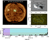 |
Fig. 2. Remote sensing properties of AR 12733. Panel (a) presents the AIA 193 Åfull-disk coronal image. The green box corresponds to the position of AR 12733. Panel (b) shows the photospheric magnetic field map of the AR, with the solid blue line outlining the MCA. Panel (c) shows AIA 1600 Åchromospheric images. Panel (d) displays the evolution curve of the ratio between the brightening regions identified in AIA 1600 Å images and the MCA regions over time. Two specific days, when AR 12733 was at the solar disk center, are highlighted with purple and blue shading. |
The chromosphere activity of the two ARs are different. AR 12671 has a larger area (approximately 400″ × 150″), a more complex magnetic field structure, more sunspots, and significantly higher chromospheric activity than AR 12733. Small-scale transient chromospheric brightenings are observed in both regions, probably caused by a microflare or other small-scale chromospheric activities (Huang et al. 2014; Dumin & Somov 2020; Madjarska et al. 2022). The difference in chromospheric activity between the two ARs is mainly due to the occurrence of flares and microflares. As discussed above, AR 12671 is associated with a higher flare occurrence rate. No GOES flares are observed in AR 12733. We regard PBA>10‰ as intense chromospheric activity. Our method reveals that all GOES flares are associated with PBA values exceeding 10‰, during the 3 days when AR 12671 was near the solar disk center. The PBA caused by small-scale non-flare activity is generally below 10‰. Therefore, we chose this threshold as an indicator of strong chromospheric activity. Each PBA peak corresponds to a chromospheric brightening event. During AR 12671 facing the Earth, the PBA exceeded 10‰ on 50 occasions and 15‰ on 20 occasions. It means that AR 12761 experienced frequent and intense chromospheric brightening events. The average PBA was 2.3‰ (see panel (h) in Fig. 1), and the PBA exceeded 2‰ (5‰) for 32% (10%) of the time. In contrast, when AR 12733 was facing the Earth, the PBA exceeded 5‰ only seven times, and the average PBA is 0.3‰ (panel (d) in Fig. 2). The PBA exceeded 2‰ for only 2.7% of the time. This indicates that the chromospheric activity of AR 12761 is more intense compared to AR 12733. Flares and microflares can cause a significant ratio increase (with brightening ratios exceeding 15‰ and 5‰). It is worth noting that when the PBA exceeds 5‰, chromospheric activity is generally accompanied by high-temperature plasma at millions of degrees (panels (e) and (g) of Fig. 1). This suggests that this chromospheric activity is most probably associated with chromospheric evaporation, because chromospheric evaporation can heat plasma to temperatures of millions or even tens of millions of degrees (Tian et al. 2015; Benz 2017) (see the introduction for more details). Given the distinct differences in the properties of the two ARs detected in the remote sensing data, the question arises of what differences might exist in their solar wind characteristics. To answer this, we compared the solar wind characteristics of the two ARs.
3.2. Comparison of solar wind characteristics of AR 12671 and AR 12733
The in situ solar wind characteristics associated with AR 12671 and AR 12733 are shown in Fig. 3. The figure, from top to bottom, presents the plasma speed and proton density, radial magnetic field, charge states of O7+/O6+ and QFe, and AHe. Dark gray shades mark the solar wind from AR 12671 and AR 12733. The O7+/O6+ in the solar wind from AR 12671 is higher than that in the solar wind from AR 12733 (see the black curve in panels (c1) and (c2)). The average (maximum) O7+/O6+ in the solar wind from AR 12671 is about 0.38 ± 0.13 (0.72). The average (maximum) O7+/O6+ in the solar wind from AR 12733 is about 0.12 ± 0.07 (0.27). The O7+/O6+ represents the temperature of the solar wind source region, indicating that AR 12671 has a higher temperature. The QFe in the solar wind associated with AR 12671 is generally greater than 11, with a maximum of 12.4 (Fig. 3, panel (c1), red curve). The QFe in the solar wind from AR 12733 is generally less than 11, as is shown in panel (c2). Panel (d1) shows that the average AHe in solar wind associated with AR 12671 is 3.90% ± 1.73%, with a maximum of 9.91%. The average AHe in the solar wind associated with AR 12733 is 0.89% ± 0.38%, with a maximum of 1.98%. Furthermore, we find that in the AR 12671 solar wind, AHe also peaks when QFe is high (marked by the shaded orange, green, and purple regions in the left panel). QFe is typically associated with the solar atmosphere’s rapid and intense heating processes. The in situ results suggest that intense heating processes in the solar atmosphere may lead to an increase in AHe in the slow solar wind, bringing it closer to the values observed in the fast solar wind. D’Amicis et al. (2021) refer to the slow solar wind with an AHe close to that of the fast solar wind as the Alfvenic slow wind. This type of wind is believed to originate from open magnetic field regions, where the heating and expansion mechanisms are similar to those in the source regions of the fast wind. Despite its lower speed, the Alfvenic slow wind shares similar properties with the fast solar wind, including magnetic field fluctuations and helium abundance, which causes its AHe value to approach that of the fast solar wind (Alterman & D’Amicis 2025; Alterman et al. 2025a,b).
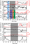 |
Fig. 3. Solar wind in situ properties. The top panel shows the in situ solar wind properties associated with AR 12671. The CME occurred from 04:00 UT on DOY 234 to 18:00 UT on DOY 235 (marked with a blue shade). The dark gray shade (DOY 236–241) represents the solar wind originating from AR 12671. The shades of orange, green, and purple in the left panel mark the AHe peak. The bottom panel presents the in situ properties of the solar wind related to AR 12733, with the dark gray shade (DOY 27–30) showing the solar wind from AR 12733. |
3.3. AHe in AR solar wind with higher and lower charge states during solar cycles 23 and 24
The results of the above case study show that the solar wind with high charge states is associated with high AHe. We further performed a statistical analysis of AHe in solar wind with higher and lower charge states during solar cycles 23 and 24. SWICS/ACE data are separated into pre-anomaly and post-anomaly periods due to an operational anomaly on August 23, 2011. Pre-anomaly data cover 1999–2009 and post-anomaly data cover 2012–2020. The Kolmogorov-Smirnov (K–S) test was used to analyze whether the AHe distribution in the two types of solar winds is the same. The statistical results are presented in Fig. 4 and surrmarized in Table 2. The first column of Fig. 4 displays the distribution of AHe in AR solar wind with QFe greater and less than 11, before and after the anomaly. The blue bars represent AR solar wind with QFe below 11, while red bars correspond to AR solar wind with QFe above 11. The second column shows the CDF (cumulative distribution function) curves of AHe in AR solar wind with QFe above and below 11, before and after the anomaly. In the two-sample K–S test, the key indicators are H, P, D, and the critical value (Dcit). When H = 1, it implies a significant difference between the two samples. The P was used to quantify the statistical significance of the distribution differences between the two groups of data. The D value corresponds to the maximum vertical distance between the two CDF curves. The value of Dcit represents the threshold that D must exceed for the test to be statistically significant at the chosen level. Therefore, the null hypothesis can be rigorously rejected only when D > Dcit and P below the chosen significance level (0.05 in this study). The statistical results indicate that AR solar wind with higher QFe tends to have higher AHe. Before the anomaly, the median AHe in solar wind with QFe>11 is about 5.0% (upper quartile 3.3%, lower quartile 6.5%), significantly higher than the 3.8% (2.8%, 5.0%) in solar wind with QFe<11. After the anomaly, the median AHe in solar wind with QFe>11 is about 4.3% (3.2%, 5.8%), higher than the 4.1% (3.1%, 5.4%) in solar wind with QFe<11. Both before and after the anomaly, the CDF curves of AHe in AR solar wind with QFe>11 lie below those with QFe<11. The H values both before and after the anomaly equal 1, the P values are well below 0.05, and the corresponding D values are 0.25>Dcit (0.04) and 0.08>Dcit (0.06), respectively.
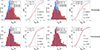 |
Fig. 4. AHe in the AR solar wind with higher and lower charge states. The top and bottom rows represent the solar wind before and after the anomaly occurred, respectively. The first column displays the distribution of AHe in AR solar wind with QFe greater and less than 11, before and after the anomaly. The blue bars represent AR solar wind with QFe less than 11. The red bars represent AR wind with QFe greater than 11. The vertical dotted blue and red lines represent the median AHe of them. The second column shows the CDF curves of AHe in AR solar wind with QFe above and below 11. The vertical dotted black line marks the maximum vertical deviation between the two curves. D represents the maximum deviation value. The third column shows the distribution of AHe in AR solar wind with O7+/O6+ above and below 0.5, before and after the anomaly. The blue bar represents O7+/O6+ less than 0.5, and the red bar represents AR wind with O7+/O6+ greater than 0.5. The fourth column displays the CDF curves of AHe in AR solar wind with O7+/O6+ above and below 0.5. |
Statistical results of AR solar wind properties before and after the anomaly.
The third column of Fig. 4 shows the distribution of AHe in AR solar wind with O7+/O6+ above and below 0.5, before and after the anomaly. The blue bars correspond to O7+/O6+ below 0.5, and the red bars represent AR wind with O7+/O6+ above 0.5. The fourth column displays the CDF curves of AHe in AR solar wind with O7+/O6+ above and below 0.5, before and after the anomaly. Our results show that before the anomaly, the median AHe in solar wind with O7+/O6+>0.5 is approximately 4.7% (2.9%, 6.7%), significantly higher than in solar wind with O7+/O6+<0.5 (around 3.9% (2.9%, 5.1%)). After the anomaly, the median AHe in solar wind with O7+/O6+>0.5 is about 4.2% (3.0%, 5.5%), a little higher than the 4.1% (3.1%,5.4%) in solar wind with O7+/O6+<0.5. Before the anomaly, the CDF curves of AHe in AR solar wind with O7+/O6+ above 0.5 lie below that for O7+/O6+ less than 0.5. Its H equals 1, P is below 0.05, and D equals 0.20, which is greater than Dcit(0.04). After the anomaly, the CDF curve of AHe in AR solar wind with O7+/O6+>0.5 nearly coincides with that of AR wind with O7+/O6+<0.5. Its H value is 0, the P value is above 0.05, and the D value is 0.03, which is less than Dcit(0.07). This indicates that there is no statistical difference in the distribution of AHe in AR solar wind with O7+/O6+ above and below 0.5, after the anomaly. This may be caused by differences in data processing introduced in response to the anomaly. Shi et al. (2025) show that the distribution and properties of O7+/O6+ changed significantly after the anomaly, especially for the lower O7+/O6+. After the anomaly, low O7+/O6+ values (less than 0.0523) were missing. Their findings suggest that the anomaly may have caused an overestimation of the lower O7+/O6+. This could lead to difficulties in distinguishing between high and low O7+/O6+ solar wind, resulting in no statistical difference between the properties of the two types of solar winds. The anomaly had a relatively small impact on QFe (Shi et al. 2025). After the anomaly, the present study shows a statistical difference in the AHe distribution between high and low QFe. Our statistical results show that the AHe differences between high charge states and low charge states solar wind are significantly larger before the anomaly than after it. We believe that the statistical results before the anomaly should be more reliable. In conclusion, the statistical results show that the AHe in AR solar wind with high charge states is generally higher than that with low charge states.
Alterman & D’Amicis (2025) investigated the relationship between AHe and solar wind speed and found a saturation value of AHe = 4.19%. This value represents the characteristic AHe of the fast wind from open magnetic field source regions (Alterman et al. 2025a). It marks the point where the upward transport of helium is no longer limited by energy. Within a closed magnetic field region, there are two main energy limitations that prevent helium from being transported upward. The first limitation is the insufficient energy input in closed magnetic field regions. In closed magnetic field regions, the energy transferred from the corona to chromosphere or transition region is limited. As a result, there is insufficient energy to accelerate both hydrogen and helium simultaneously. The FIP of helium is higher than that of hydrogen. This means that helium requires more energy to be ionized. Since hydrogen is more easily ionized, the available energy in closed magnetic field regions preferentially accelerates hydrogen. Helium can only be accelerated by the remaining energy once the hydrogen density decreases. This leads to a generally lower AHe in closed magnetic field regions, typically below 4%, with substantial numerical fluctuations. In comparison, open magnetic field regions provide a much higher energy supply. This allows for the simultaneous ionization and acceleration of both hydrogen and helium. Helium does not need to wait for hydrogen to escape or rely on energy transfer from hydrogen. It can directly gain sufficient energy through Alfvenic waves, allowing it to escape the region and maintain a high abundance. This process effectively bypasses the “energy-priority supply” limitation present in closed magnetic field regions. The second limitation is energy dissipation and matter retention in magnetic loops. The magnetic field in closed magnetic regions is ring-shaped. Plasma within the loop cannot escape directly. It must undergo a cycle of “heating-cooling-reheating” within the loop. Plasma in a closed loop dissipates energy continuously through radiation and thermal conduction, which means that even if helium is initially heated, it may not escape the loop’s confinement due to energy loss. Only when the closed magnetic field is “intermittently open“ (for example during magnetic reconnection) can the plasma escape. However, by this time, some of the helium’s energy may have already dissipated, making it difficult for its abundance to reach 4%. Open magnetic field regions completely avoid this limitation. Without the constraint of closed magnetic field lines, helium, after being heated, can be directly transported outward along the magnetic field lines with minimal energy dissipation. The “continuously open” nature of these regions allows helium to be transported upward efficiently and stably, without needing to wait for intermittent openings. This ensures that the helium abundance naturally exceeds 4%. Their study suggests that solar wind with AHe below the saturation value originates from source regions with closed magnetic fields. In these regions, the energy input is insufficient to transport helium to the corona continuously. In contrast, for solar wind with AHe above 4%, it indicates that the source region possesses a sustained open magnetic field and sufficient energy input, allowing it to transport high-helium material to the corona continually.
Our statistical results are consistent with these findings. We find that before and after the anomaly, the median AHe in AR solar wind with QFe less than 11 is approximately 3.82% and 4.13%, respectively. O7+/O6+ less than 0.5 is approximately 3.87% before the anomaly. The low charge states indicate that these source regions lack intense activity and are not able to efficiently transport high-helium material to the upper atmosphere. Thus, their corresponding AHe are lower than 4.19%. In contrast, for AR solar wind with QFe greater than 11, the median AHe before and after the anomaly is approximately 5.04% and 4.27%, respectively. The median AHe for O7+/O6+ greater than 0.5 is about 4.67%, before the anomaly. These source regions experience frequent intense activity, providing enough energy to continuously transport high-helium material to the upper atmosphere, leading to AHe greater than 4.19%.
4. Discussion
Our case study demonstrates that the AHe and charge states are higher for the solar wind associated with greater chromospheric activity. In addition, our statistical analysis shows that the AHe in solar wind with higher charge states is higher than that in the solar wind with lower charge states. The above results can be explained reasonably well by the scenario presented in Fig. 5. The main idea illustrated in this figure is that chromospheric activity, primarily driven by chromospheric evaporation processes, can heat and transport plasma associated with higher AHe from the lower solar atmosphere to the corona and solar wind. The energy released by magnetic reconnection during flares or microflares in the corona accelerates high-energy electrons (step 1 in Fig. 5). High-energy electrons are transported downward to the footpoints and heat the chromospheric material to high temperatures (steps 2 and 3). Significant brightenings, for example the flare ribbons, seen especially well in the Hα and 1600 Å passbands, can be observed in the chromosphere. The overpressure caused by chromospheric heating drives the heated plasma upward along magnetic loops (step 4). The heated chromospheric material with high temperatures and high AHe fills the coronal loops (shown in light green) (step 5). Finally, these coronal loops could reconnect with the surrounding open magnetic field lines, allowing high AHe material to escape into the solar wind (step 6). The scenario is consistent with the AIA observations, such as the obvious brightenings seen in the AIA 1600 Å images and the high-temperature plasma of 9–20 MK detected by the DEM method.
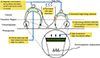 |
Fig. 5. Cartoon illustrating the plasma heating in the lower atmosphere by chromospheric evaporation and the transmission of the heated plasma upward into the corona and the solar wind. The chromospheric evaporation is triggered by the energy released during magnetic reconnection in the corona. The downward arrows represent the high-energy electrons being accelerated. |
The above-described scenario is strongly supported by findings related to ICMEs. Previous studies have shown that the ICME materials with higher AHe and charge states are generated by chromospheric evaporation processes. Fu et al. (2020) found that during flares, chromospheric material is transported to the eruption flux rope through chromospheric evaporation, supplying mass to the CME. They found that the AHe is significantly higher in the associated ICME. For CMEs without flares, accompanied by low-class (B class), medium-class (C class), and high-class (M and X class) flares, AHe is 3.03%, 4.93%, 5.30%, and 8.25%, respectively (Zhai et al. 2022). As the flare class increases, the proportion of high AHe material from chromospheric evaporation in CMEs rises significantly. For CMEs accompanied by low-class (B class), medium-class (C class), and high-class (M and X class) flares, the proportions of plasma generated by chromospheric evaporation are 14.5%, 43.7%, and 68.2%, respectively (Fu et al. 2023). These results demonstrate that the plasma heated by the chromospheric evaporation is associated with high AHe and charge states. Therefore, it is reasonable to assume that chromospheric evaporation can inject high-temperature, high AHe plasma into the corona and solar wind.
The ARs with intense chromospheric activity, and thus more intense chromospheric evaporation, may transport higher temperature and higher AHe chromospheric material into the upper atmosphere and solar wind. As a result, solar winds with higher charge states are statistically associated with a high AHe. However, not all high charge state solar wind is associated with high AHe, and the distribution of AHe in high and low charge state solar winds shows considerable overlap. This is because the AHe in the solar wind is influenced by multiple factors, such as gravity stratification, coulomb collisions, and the global topology of the solar magnetic field (Alterman & Kasper 2019; Yogesh et al. 2021, 2022; Alterman et al. 2021; Alterman & D’Amicis 2025; Alterman et al. 2025a,b).
The variation of AHe in AR solar wind during the different solar cycle phases, as well as the higher AHe in AR solar wind compared to QS solar wind, can also be reasonably explained by the above scenario. During solar maximum, more than half of the near-Earth solar wind comes from ARs (Fu et al. 2015; Shi et al. 2024). As is well known, during the solar maximum, the number of ARs increases and the magnetic field activity becomes more intense. This leads to more frequent chromospheric evaporation processes, as is illustrated by the cartoon in Fig. 5. This injects more hotter and higher AHe plasma into the upper atmosphere and solar wind. In contrast, chromospheric evaporation decreases during the solar minimum. Consequently, AHe in the solar wind decreases during the solar minimum.
Previous studies have demonstrated that AHe is higher in AR solar wind than in the QS solar wind (Fu et al. 2018). We propose that this occurs because chromospheric evaporation is more significant in ARs. The magnetic field in ARs is stronger and more active, leading to a more frequent chromospheric evaporation process. In QS regions, chromospheric evaporation also happens, but on a smaller scale (Frogner et al. 2020). As a result, AHe in AR solar wind is higher than that in QS solar wind.
5. Summary and conclusions
The present study explores the relationship between the activity and characteristics of the ARs and their associated solar wind. The AHe in the AR solar wind with higher and lower charge states during solar cycles 23 and 24 are also analyzed statistically. We find that:
The AR with greater chromospheric activity has higher AHe in its associated solar wind. To be specific, when the AR with strong chromospheric activity (AR 12671) was facing the Earth, the PBA exceeded 2‰ (5‰) for 32% (10%) of the time. Additionally, the PBA exceeds 10‰ (15‰) 50 (20) times, and the average PBA is 2.3‰ (see panel (h) in Figure 1). In contrast, when the AR with weak chromospheric activity (AR 12733) was facing the Earth, the PBA exceeded 2‰ for only 2.7% of the time. The PBA exceeds 5‰ and 10‰ for only 7 and 0 times, and the average PBA is 0.3‰ (panel (d) in Figure 2). The average AHe in solar wind associated with AR 12671 is 4.00% ± 1.58%. The average AHe in the solar wind associated with AR 12733 is 0.89% ± 0.38%.
Statistical analysis of AR solar wind during solar cycles 23 and 24 shows that solar wind with high charge states is associated with high AHe. Specifically, before the anomaly, the median AHe in solar wind with QFe>11 is about 5.0% (upper quartile 3.3%, lower quartile 6.5%), significantly higher than the 3.8% (2.8%, 5.0%) in solar wind with QFe<11. After the anomaly, the median AHe in solar wind with QFe>11 is about 4.3% (3.2%, 5.8%), higher than the 4.1% (3.1%, 5.4%) in solar wind with QFe<11. Both the H values before and after the anomaly equal 1, the P values are well below 0.05, and the corresponding D values are 0.25>Dcit (0.04) and 0.08>Dcit (0.06), respectively. Before the anomaly, the median AHe in solar wind with O7+/O6+>0.5 is approximately 4.7% (2.9%, 6.7%), significantly higher than in solar wind with O7+/O6+<0.5 (around 3.9% (2.9%, 5.1%)). Its H equals 1, P is below 0.05, and D equals 0.20, which is greater than Dcit(0.04). The statistical results are presented in Table 2.
Our results suggest that chromospheric evaporation processes may play a key role in enhancing AHe in solar wind. The present study indicates that chromospheric activity, primarily chromospheric evaporation processes, can heat and transport lower solar atmosphere materials associated with higher AHe to the corona and solar wind. The variation of AHe in AR solar wind with the solar activity phases and the higher AHe in AR solar wind compared to QS solar wind can be reasonably explained by the above scenario.
Acknowledgments
The author sincerely thank the referee for helping improve the quality of our manuscript. We thanks the SWICS, SWEPAM instrument teams, and the ACE Science Center for providing the data. The AIA and HMI data are used courtesy of NASA/SDO, the AIA and HMI teams, and JSOC. Analysis of Wind SWE observations is supported by NASA grant NNX09AU35G. We thank the SEW and Wind teams for the use of their data. This research is supported by the National Natural Science Foundation of China (12473058, 42230203). M.M. acknowledges the support of the Brain Pool program funded by the Ministry of Science and ICT through the National Research Foundation of Korea (RS-2024-00408396) and DFG grant WI 3211/8-2, project number 452856778.
References
- Aellig, M. R., Lazarus, A. J., & Steinberg, J. T. 2001, Geophys. Res. Lett., 28, 2767 [NASA ADS] [CrossRef] [Google Scholar]
- Alterman, B. L., & D’Amicis, R. 2025, ApJ, 982, L40 [Google Scholar]
- Alterman, B. L., & Kasper, J. C. 2019, ApJ, 879, L6 [Google Scholar]
- Alterman, B. L., Kasper, J. C., Leamon, R. J., & McIntosh, S. W. 2021, Sol. Phys., 296, 67 [Google Scholar]
- Alterman, B. L., Rivera, Y. J., Lepri, S. T., & Raines, J. M. 2025a, A&A, 694, A265 [NASA ADS] [CrossRef] [EDP Sciences] [Google Scholar]
- Alterman, B. L., Rivera, Y. J., Lepri, S. T., Raines, J. M., & D’Amicis, R. 2025b, A&A, 700, A23 [NASA ADS] [CrossRef] [EDP Sciences] [Google Scholar]
- Antonucci, E., Gabriel, A. H., & Dennis, B. R. 1984, ApJ, 287, 917 [NASA ADS] [CrossRef] [Google Scholar]
- Asplund, M., Grevesse, N., Sauval, A. J., & Scott, P. 2009, ARA&A, 47, 481 [NASA ADS] [CrossRef] [Google Scholar]
- Basu, S., & Antia, H. M. 2008, Phys. Rep., 457, 217 [Google Scholar]
- Battaglia, A. F., Krucker, S., Veronig, A. M., et al. 2024, A&A, 691, A172 [NASA ADS] [CrossRef] [EDP Sciences] [Google Scholar]
- Benz, A. O. 2017, Liv. Rev. Sol. Phys., 14, 2 [Google Scholar]
- Chae, J., Wang, H., Lee, C.-Y., Goode, P. R., & Schühle, U. 1998, ApJ, 504, L123 [NASA ADS] [CrossRef] [Google Scholar]
- Cheung, M. C. M., Boerner, P., Schrijver, C. J., et al. 2015, ApJ, 807, 143 [Google Scholar]
- Chifor, C., Isobe, H., Mason, H. E., et al. 2008, A&A, 491, 279 [NASA ADS] [CrossRef] [EDP Sciences] [Google Scholar]
- D’Amicis, R., Alielden, K., Perrone, D., et al. 2021, A&A, 654, A111 [NASA ADS] [CrossRef] [EDP Sciences] [Google Scholar]
- Del Zanna, G., Storey, P. J., Badnell, N. R., & Andretta, V. 2020, ApJ, 898, 72 [Google Scholar]
- Dere, K. P. 1994, Adv. Space Res., 14, 13 [Google Scholar]
- Dumin, Y. V., & Somov, B. V. 2020, Sol. Phys., 295, 92 [Google Scholar]
- Feldman, U. 1992, Phys. Scr., 46, 202 [CrossRef] [Google Scholar]
- Feldman, U., & Widing, K. G. 2003, Space Sci. Rev., 107, 665 [CrossRef] [Google Scholar]
- Feldman, W. C., Asbridge, J. R., Bame, S. J., & Gosling, J. T. 1978, J. Geophys. Res., 83, 2177 [NASA ADS] [CrossRef] [Google Scholar]
- Fisher, G. H., Canfield, R. C., & McClymont, A. N. 1985, ApJ, 289, 414 [NASA ADS] [CrossRef] [Google Scholar]
- Fletcher, L., Dennis, B. R., Hudson, H. S., et al. 2011, Space Sci. Rev., 159, 19 [Google Scholar]
- Frogner, L., Gudiksen, B. V., & Bakke, H. 2020, A&A, 643, A27 [NASA ADS] [CrossRef] [EDP Sciences] [Google Scholar]
- Fu, H., Li, B., Li, X., et al. 2015, Sol. Phys., 290, 1399 [CrossRef] [Google Scholar]
- Fu, H., Madjarska, M. S., Li, B., Xia, L., & Huang, Z. 2018, MNRAS, 478, 1884 [CrossRef] [Google Scholar]
- Fu, H., Harrison, R. A., Davies, J. A., et al. 2020, ApJ, 900, L18 [Google Scholar]
- Fu, H., Shi, X., Huang, Z., Qi, Y., & Xia, L. 2023, ApJ, 956, 129 [Google Scholar]
- Garcia, H. A. 1994, Sol. Phys., 154, 275 [NASA ADS] [CrossRef] [Google Scholar]
- Gloeckler, G., Cain, J., Ipavich, F. M., et al. 1998, Space Sci. Rev., 86, 497 [NASA ADS] [CrossRef] [Google Scholar]
- Graham, D. R., & Cauzzi, G. 2015, ApJ, 807, L22 [NASA ADS] [CrossRef] [Google Scholar]
- Grevesse, N., & Sauval, A. J. 1998, Space Sci. Rev., 85, 161 [Google Scholar]
- Gupta, G. R., & Tripathi, D. 2015, ApJ, 809, 82 [Google Scholar]
- Hannah, I. G., Hudson, H. S., Battaglia, M., et al. 2011, Space Sci. Rev., 159, 263 [NASA ADS] [CrossRef] [Google Scholar]
- Hirayama, T. 1974, Sol. Phys., 34, 323 [Google Scholar]
- Huang, Z., Madjarska, M. S., Xia, L., et al. 2014, ApJ, 797, 88 [Google Scholar]
- Kasper, J. C., Stevens, M. L., Lazarus, A. J., Steinberg, J. T., & Ogilvie, K. W. 2007, ApJ, 660, 901 [Google Scholar]
- Kasper, J. C., Stevens, M. L., Korreck, K. E., et al. 2012, ApJ, 745, 162 [Google Scholar]
- Lemen, J. R., Title, A. M., Akin, D. J., et al. 2012, Sol. Phys., 275, 17 [Google Scholar]
- Lepping, R. P., Acũna, M. H., Burlaga, L. F., et al. 1995, Space Sci. Rev., 71, 207 [Google Scholar]
- Li, W., & Wang, J. 1998, ASP Conf. Ser., 150, 401 [Google Scholar]
- Ma, C., Fu, H., Huang, Z., et al. 2022, ApJ, 939, 20 [Google Scholar]
- Madjarska, M. S., Mackay, D. H., Galsgaard, K., Wiegelmann, T., & Xie, H. 2022, A&A, 660, A45 [NASA ADS] [CrossRef] [EDP Sciences] [Google Scholar]
- Masson, S., Pariat, E., Aulanier, G., & Schrijver, C. J. 2009, ApJ, 700, 559 [Google Scholar]
- McIntosh, S. W. 2012, Space Sci. Rev., 172, 69 [NASA ADS] [CrossRef] [Google Scholar]
- McIntosh, S. W., Kiefer, K. K., Leamon, R. J., Kasper, J. C., & Stevens, M. L. 2011, ApJ, 740, L23 [NASA ADS] [CrossRef] [Google Scholar]
- Milligan, R. O., Gallagher, P. T., Mathioudakis, M., et al. 2006a, ApJ, 638, L117 [NASA ADS] [CrossRef] [Google Scholar]
- Milligan, R. O., Gallagher, P. T., Mathioudakis, M., & Keenan, F. P. 2006b, ApJ, 642, L169 [NASA ADS] [CrossRef] [Google Scholar]
- Ogilvie, K. W., & Hirshberg, J. 1974, J. Geophys. Res., 79, 4595 [Google Scholar]
- Ogilvie, K. W., Chornay, D. J., Fritzenreiter, R. J., et al. 1995, Space Sci. Rev., 71, 55 [Google Scholar]
- Pesnell, W. D., Thompson, B. J., & Chamberlin, P. C. 2012, Sol. Phys., 275, 3 [Google Scholar]
- Priest, E. R., & Longcope, D. W. 2017, Sol. Phys., 292, 25 [Google Scholar]
- Raouafi, N. E., Patsourakos, S., Pariat, E., et al. 2016, Space Sci. Rev., 201, 1 [Google Scholar]
- Saqri, J., Veronig, A. M., Battaglia, A. F., et al. 2024, A&A, 683, A41 [NASA ADS] [CrossRef] [EDP Sciences] [Google Scholar]
- Schou, J., Scherrer, P. H., Bush, R. I., et al. 2012, Sol. Phys., 275, 229 [Google Scholar]
- Shen, Y. 2021, Proc. R. Soc. Lond. Ser. A, 477, 217 [NASA ADS] [Google Scholar]
- Shi, X., Fu, H., Huang, Z., et al. 2024, ApJ, 972, 54 [Google Scholar]
- Shi, X., Fu, H., Huang, Z., et al. 2025, arXiv e-prints [arXiv:2510.08975] [Google Scholar]
- Shibata, K., Nakamura, T., Matsumoto, T., et al. 2007, Science, 318, 1591 [Google Scholar]
- Steinberg, J. T., Lazarus, A. J., Ogilvie, K. W., Lepping, R., & Byrnes, J. 1996, Geophys. Res. Lett., 23, 1183 [Google Scholar]
- Stone, E. C., Frandsen, A. M., Mewaldt, R. A., et al. 1998, Space Sci. Rev., 86, 1 [Google Scholar]
- Su, Y., Veronig, A. M., Hannah, I. G., et al. 2018, ApJ, 856, L17 [NASA ADS] [CrossRef] [Google Scholar]
- Tian, H., Young, P. R., Reeves, K. K., et al. 2015, ApJ, 811, 139 [NASA ADS] [CrossRef] [Google Scholar]
- Veronig, A., Vršnak, B., Dennis, B. R., et al. 2002, A&A, 392, 699 [NASA ADS] [CrossRef] [EDP Sciences] [Google Scholar]
- von Steiger, R., & Schwadron, N. A. 2000, ASP Conf. Ser., 206, 54 [Google Scholar]
- Yogesh, Chakrabarty, D., & Srivastava, N. 2021, MNRAS, 503, L17 [NASA ADS] [CrossRef] [Google Scholar]
- Yogesh, Chakrabarty, D., & Srivastava, N. 2022, MNRAS, 513, L106 [Google Scholar]
- Zhai, H., Fu, H., Huang, Z., & Xia, L. 2022, ApJ, 928, 136 [Google Scholar]
Appendix A: Intensity distribution
Figure A.1 shows the intensity distribution of all pixels within the MCA contoured by the blue solid line in panel (d) of Fig 1 in the main text.
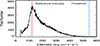 |
Fig. A.1. Histogram of intensity distribution within the MCAs. The red line on the left indicates the reference intensity. It represents the intensity value corresponding to the maximum number of pixels. The blue line on the right marks the threshold. |
Appendix B: Temperature distribution
DEM analysis on the area outlined in the white box in panels (d) and (f) of Fig 1 in the main text.
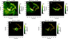 |
Fig. B.1. EM of the C 7.0 flare. Panel (a)–(e) represents EM of 1–2.5 MK, 2.5–4.5 MK, 5–8 MK, 9–20 MK, and 20–30 MK, respectively. |
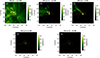 |
Fig. B.2. EM of the small-scale chromospheric brightening events. Panel (a)–(e) represents EM of 1–2.5 MK, 2.5–4.5 MK, 5–8 MK, 9–20 MK, and 20–30 MK, respectively. |
All Tables
All Figures
|
Fig. 1. Remote sensing properties of AR 12671. Panel (a) displays the AIA 193 Å full-disk coronal image. The green box corresponds to the position of AR 12671. Panel (b) shows the AIA 193 Å coronal map of AR 12671. Panel (c) displays the photospheric magnetic field map of AR 12671, with the solid blue line outlining the MCA. Panel (d) shows the AIA 1600 Å image corresponding to the C 7.0 flare that occurred at 21:45 UT on August 19, 2017. Panel (f) shows a small-scale chromospheric brightening event that occurred at 18:40 UT on August 19, 2017. The brightening regions are outlined by the solid red line. Panel (e) shows the 2.5–4.5 MK EM of the area outlined with a white box in Panel (d), with the orange line contouring the brightening regions. Panel (h) displays the evolution curve of the PBA over time. The vertical axis represents the ratio value of brightening areas and the whole AR ×1000. The three days of AR 12671 at the center of the solar disk are highlighted with purple, blue, and green shades, respectively. Vertical red lines (&#Xtextcircled;1–&#Xtextcircled;5) mark the time of five GOSE flares. The vertical blue line marks the time of small-scale chromospheric brightening. We can see that AR 12671 exhibited significant chromospheric activity during its time at the solar disk center. |
| In the text | |
|
Fig. 2. Remote sensing properties of AR 12733. Panel (a) presents the AIA 193 Åfull-disk coronal image. The green box corresponds to the position of AR 12733. Panel (b) shows the photospheric magnetic field map of the AR, with the solid blue line outlining the MCA. Panel (c) shows AIA 1600 Åchromospheric images. Panel (d) displays the evolution curve of the ratio between the brightening regions identified in AIA 1600 Å images and the MCA regions over time. Two specific days, when AR 12733 was at the solar disk center, are highlighted with purple and blue shading. |
| In the text | |
|
Fig. 3. Solar wind in situ properties. The top panel shows the in situ solar wind properties associated with AR 12671. The CME occurred from 04:00 UT on DOY 234 to 18:00 UT on DOY 235 (marked with a blue shade). The dark gray shade (DOY 236–241) represents the solar wind originating from AR 12671. The shades of orange, green, and purple in the left panel mark the AHe peak. The bottom panel presents the in situ properties of the solar wind related to AR 12733, with the dark gray shade (DOY 27–30) showing the solar wind from AR 12733. |
| In the text | |
|
Fig. 4. AHe in the AR solar wind with higher and lower charge states. The top and bottom rows represent the solar wind before and after the anomaly occurred, respectively. The first column displays the distribution of AHe in AR solar wind with QFe greater and less than 11, before and after the anomaly. The blue bars represent AR solar wind with QFe less than 11. The red bars represent AR wind with QFe greater than 11. The vertical dotted blue and red lines represent the median AHe of them. The second column shows the CDF curves of AHe in AR solar wind with QFe above and below 11. The vertical dotted black line marks the maximum vertical deviation between the two curves. D represents the maximum deviation value. The third column shows the distribution of AHe in AR solar wind with O7+/O6+ above and below 0.5, before and after the anomaly. The blue bar represents O7+/O6+ less than 0.5, and the red bar represents AR wind with O7+/O6+ greater than 0.5. The fourth column displays the CDF curves of AHe in AR solar wind with O7+/O6+ above and below 0.5. |
| In the text | |
|
Fig. 5. Cartoon illustrating the plasma heating in the lower atmosphere by chromospheric evaporation and the transmission of the heated plasma upward into the corona and the solar wind. The chromospheric evaporation is triggered by the energy released during magnetic reconnection in the corona. The downward arrows represent the high-energy electrons being accelerated. |
| In the text | |
|
Fig. A.1. Histogram of intensity distribution within the MCAs. The red line on the left indicates the reference intensity. It represents the intensity value corresponding to the maximum number of pixels. The blue line on the right marks the threshold. |
| In the text | |
|
Fig. B.1. EM of the C 7.0 flare. Panel (a)–(e) represents EM of 1–2.5 MK, 2.5–4.5 MK, 5–8 MK, 9–20 MK, and 20–30 MK, respectively. |
| In the text | |
|
Fig. B.2. EM of the small-scale chromospheric brightening events. Panel (a)–(e) represents EM of 1–2.5 MK, 2.5–4.5 MK, 5–8 MK, 9–20 MK, and 20–30 MK, respectively. |
| In the text | |
Current usage metrics show cumulative count of Article Views (full-text article views including HTML views, PDF and ePub downloads, according to the available data) and Abstracts Views on Vision4Press platform.
Data correspond to usage on the plateform after 2015. The current usage metrics is available 48-96 hours after online publication and is updated daily on week days.
Initial download of the metrics may take a while.