| Issue |
A&A
Volume 706, February 2026
|
|
|---|---|---|
| Article Number | A15 | |
| Number of page(s) | 12 | |
| Section | Cosmology (including clusters of galaxies) | |
| DOI | https://doi.org/10.1051/0004-6361/202555896 | |
| Published online | 27 January 2026 | |
Generative models of 21 cm Epoch of Reionisation lightcones with 3D scattering transforms
1
Laboratoire de Physique de l’ENS, ENS, Université PSL, CNRS, Sorbonne Université, Universitée Paris Cité 75005 Paris, France
2
LERMA, Observatoire de Paris, PSL Research University, CNRS, Sorbonne Université F-75014 Paris, France
3
Department of Physics, Blackett Laboratory, Imperial College London London SW7 2AZ, UK
★ Corresponding author: This email address is being protected from spambots. You need JavaScript enabled to view it.
Received:
11
June
2025
Accepted:
26
November
2025
Abstract
The 21 cm signal from the Epoch of Reionisation (EoR) is observed as a 3D dataset known as a lightcone, consisting of two spatial sky plane axes and a redshift (frequency) axis. Owing to its strongly non-Gaussian nature, fully characterising this signal requires summary statistics that go beyond two-point power spectra statistics. Recent developments in astrophysics, particularly in the context of the Galactic interstellar medium, demonstrate the efficacy of scattering transforms–novel summary statistics–to characterise fields with highly non-Gaussian properties. In particular, these statistics allow us to construct maximum-entropy generative models, even from a single target map, from which we can sample new, almost statistically identical realisations of a given process. Motivated by these advances, we extended the scattering transform formalism from 2D datasets to 3D EoR lightcones. To this end, we introduced a 3D wavelet set from the tensor product of 2D isotropic wavelets in the sky plane domain and 1D wavelets in the redshift domain. To test how well this 3D scattering transform can characterise an EoR lightcone, we constructed a maximum entropy generative model of EoR lightcones, which we quantitatively validated by comparing the new synthesised EoR lightcones with the single target lightcone from which the model is defined. Using independent statistics such as the power spectrum, histograms, and Minkowski functionals, we show that the synthesised lightcones agree very well with the target lightcone, both statistically and visually. The success of these generative models in quickly generating EoR lightcones, which can be extended to a broad range of 3D and heterogeneous 2+1D data, opens up a variety of potential applications, from forward modelling to uncertainty quantification.
Key words: instrumentation: interferometers / methods: statistical / cosmology: observations / early Universe / dark ages / reionization / first stars
© The Authors 2026
 Open Access article, published by EDP Sciences, under the terms of the Creative Commons Attribution License (https://creativecommons.org/licenses/by/4.0), which permits unrestricted use, distribution, and reproduction in any medium, provided the original work is properly cited.
This article is published in open access under the Subscribe to Open model. This email address is being protected from spambots. You need JavaScript enabled to view it. to support open access publication.
1. Introduction
The Epoch of Reionisation (EoR) is a critical transition in the history of the Universe, marking the emergence of the first stars and the eventual ionisation of the once-neutral intergalactic medium (IGM). Indirect observations of the EoR from the cosmic microwave background (CMB) (Planck Collaboration XLVII 2016; Gorce et al. 2018) and the Gunn-Peterson trough in quasar spectra (Fan et al. 2006; Becker et al. 2015; Bosman et al. 2018; Qin et al. 2021), constrain the timing of the EoR between redshifts 14 ≳ z ≳ 5.3.
Ground–based CMB measurements provide a complementary EoR probe: South Pole Telescope (SPT) analyses constrain the duration to  (< 4.1 at 95% C.L.), and a cosmology–dependent reanalysis finds Δzre, 50 < 4.3 with
  (Reichardt et al. 2021; Gorce et al. 2022); although the Atacama Cosmology Telescope (ACT) has not yet detected the trispectrum, it sets an upper limit and roadmap for future detections (MacCrann et al. 2024), reinforcing the high-ℓ trispectrum as a viable, complementary EoR probe (Kumar et al. 2025).
While these indirect observations offer loose timings of the EoR, they do not constrain the sources responsible for the EoR, nor the state of the IGM, for which a direct probe is needed. The redshifted 21 cm signal, resulting from the hyperfine transition in neutral hydrogen during the EoR, presents a promising direct observational probe (observed by radio interferometers between ∼100 MHz and 200 MHz) for a comprehensive study of this epoch.
Observations of the 21 cm signal (EoR signal, henceforth) by radio interferometers must contend with foregrounds such as synchrotron emission from diffuse clouds in the Galaxy, noise arising from the antennas, and systematics such as mode-mixing arising from the chromatic nature of radio interferometers. All of these contaminants are orders of magnitude stronger in total variance than the signal itself (Shaver et al. 1999; Jelić et al. 2008; Hothi et al. 2021).
The cylindrically averaged power spectrum of a radio interferometer observation (Fig. 1) has three distinct regions in the k∥ − k⊥ plane1 (Datta et al. 2010; Vedantham et al. 2012). The first region, located at low k∥, is dominated by astrophysical foregrounds. These foregrounds include Galactic emission, arising from free-free bremsstrahlung and diffuse synchrotron emission, as well as extragalactic synchrotron emission arising from sources such as radio haloes and clusters (Jelić et al. 2008; Hothi et al. 2021). The second region is the foreground wedge, which arises from the chromatic nature of the instrument: the interferometer’s point spread function (PSF) is frequency dependent, leading to mode mixing between k⊥ and k∥ and causing the foreground emission to leak to higher k∥ (Liu et al. 2014). Bright sources entering the side lobes of the interferometer’s PSF also contribute to the emission within the wedge, all of which are bound by the horizon2. The third region is the EoR window, where foregrounds and instrumental effects are subdominant (there is little to no contribution on these scales) to the noise and EoR signal (see Munshi et al. 2025 for a more comprehensive overview of the wedge).
The EoR signal is expected to be highly non-Gaussian, and this non-Gaussian information is important to constrain both the astrophysics of this epoch and the progression of reionisation (Shimabukuro et al. 2017; Watkinson et al. 2022; Tiwari et al. 2022). To fully characterise the signal requires statistics beyond the power spectrum.
Scattering transforms (STs) have emerged as a novel set of summary statistics constructed by successive wavelet convolutions and the application of non-linear operators such as modulus (Mallat 2011; Bruna & Mallat 2012). They have emerged as powerful low-variance statistics to characterise non-Gaussian processes and have already been successfully applied to various topics, including the study of the interstellar medium (Allys et al. 2019; Regaldo-Saint Blancard et al. 2020; Lei & Clark 2023); weak lensing (Cheng et al. 2020); the large-scale structure of the Universe for 2D (Allys et al. 2020) and 3D data (Eickenberg et al. 2022; Valogiannis & Dvorkin 2022; Régaldo-Saint Blancard et al. 2024); and more recently, to the EoR (Greig et al. 2022; Zhao et al. 2024; Hothi et al. 2024; Prelogović & Mesinger 2024; Shimabukuro et al. 2025).
An advantage of ST statistics is that they can be used to build generative models of physical processes within the framework of maximum entropy models. Such models, parametrised by the ST statistics themselves, efficiently approximate complex non-Gaussian physical fields, even when constructed from a single sample (Allys et al. 2020; Cheng et al. 2023; Mousset et al. 2024; Campeti et al. 2025). Scattering transforms (STs) have also been used in the context of EoR to build diffusion models, using U-Nets, and outperform generative adversarial networks when applied to 2D EoR fields (Zhao et al. 2023).
The ability to generate realistic realisations of various processes under ST constraints has led to the development of new component separation algorithms. These ST-based component separations have already been successfully applied directly to observational data, exploiting the non-Gaussian properties of the components within the data, without physically driven priors on the component of interest (Regaldo-Saint Blancard et al. 2021; Delouis et al. 2022; Auclair et al. 2024). However, these previous algorithms have only been applied to 2D data. For EoR studies, this formalism must be extended to 3D EoR lightcones. This in turn requires reliance on ST statistics that can adequately describe such data, the development of which is the purpose of this paper. This work therefore extends ST generative models to 3D EoR data and quantitatively validates their quality.
To construct such 3D ST statistics, the first step is to introduce a relevant set of wavelets that characterise the different regions of the k∥ − k⊥ plane (see Fig. 1). In previous 3D ST applications, wavelet sets typically probe extended regions of the k∥ − k⊥ plane, thus mixing regions where the foregrounds are dominant and subdominant (see, for example, Eickenberg et al. 2022). This is problematic because mixing regions where foregrounds are dominant with subdominant regions is detrimental to the efficient extraction of information from the EoR signal (Blamart & Liu 2025). To avoid this drawback, we constructed a new set of 3D wavelets from the tensor product of 1D wavelets along the k∥ axis and 2D isotropic wavelets along the sky axes (kx, ky). We then used this new wavelet set to construct 3D ST statistics, which we in turn used to construct a generative model of EoR lightcones, the quality of which was assessed quantitatively. The ST model is built from a single simulated EoR lightcone; we compared its statistical properties with those of the simulation using several independent and complementary statistics.
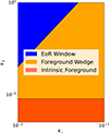 |
Fig. 1. Schematic of the cylindrically-averaged power spectrum of an observed EoR lightcone, with the three distinct regions highlighted. |
The paper is structured as follows. Section 2 outlines the simulations used. Section 3 presents the 3D scattering transforms. Section 4 describes the generative model built from scattering transforms. Section 5 compares the synthesised lightcones with the target EoR lightcones.
2. LoReLi II simulation
The simulation used in this work is from the LoReLi II (LOw REsolution LIcorice) database (Meriot & Semelin 2024; Meriot et al. 2025). This database is a collection of Licorice simulations designed to study the EoR signal (Semelin et al. 2007, 2017).
The LoReLi II database comprises 9828 simulations of the EoR signal brightness temperature and explores a four-parameter space: the gas-to-star conversion timescale, the minimum halo mass for star formation, the escape fraction of UV radiation, and the X-ray production efficiency, while keeping the cosmological parameters constant at {H0: 67.8 km/s/Mpc, Ω0: 0.308, Ωb: 0.0484, ΩΛ: 0.692, and σ8: 0.815}. This setup allows for a detailed exploration of the astrophysical processes during reionisation without the confounding effects of varying cosmology.
In this paper, the ST generative model is built from a single LoReLi simulation of a lightcone. The astrophysical parameters of the lightcone, which we refer to as the target lightcone, are the log10 of the minimum halo mass, Mmin = 8.0; the X-ray luminosity fraction, fx = 0.1; the hard X ray fraction,  = 0.2; the gas conversion timescale for star formation in units of 10 Myr, τ = 8191.9; and the ionising escape fraction, fesc, post = 0.275.
This lightcone spans a redshift range of 23 ≤ z ≤ 5. The xy-plane (the 2D sky) contains 2562 pixels, and the z-domain contains 3072 redshift channels between z = 23 and z = 5. To reduce the computational cost and limit the z evolution over the lightcone, we downgraded it from 2562 pixels to 1282 pixels in the xy plane, and restricted the z values to 9.5 ≤ z ≤ 8.5 (frequency bandwidth δν ∼ 14 MHz), corresponding to 170 pixels in the z domain, for a final data cube of (128, 128, 170) pixels. If the ST statistics were estimated on the initial lightcone, their statistical properties would evolve with z, whereas we approximated only limited z-evolution in the final constructed lightcone. However, we note that a lightcone with a larger redshift range could be built by stacking models constructed with a more limited redshift range (Blamart & Liu 2025).
3. Scattering transforms for 3D lightcones
3.1. Wavelets for 3D lightcones
In this paper, we introduce a wavelet set that characterises the k∥ − k⊥ plane by performing a tensor product between wavelet sets defined on different axes. The first is a 1D wavelet set defined in kz, denoted by ∥, and the second is a 2D isotropic wavelet set defined in the (kx, ky) plane, denoted by ⊥. To simplify notation, we define the modulus wavenumbers in the two ∥ and ⊥ directions by k∥ = |kz| and  .
.
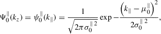
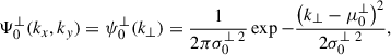
The L1-normalised mother wavelet of the 1D ∥ wavelet set is defined as
 (1)
(1)
where μ0∥ is the central wavenumber of the mother wavelet in Fourier space, and σ0∥ its width. Here, we denote the wavelets in the 3D (kx, ky, kz) space with Ψ and the wavelets in the 2D (k∥, k⊥) cylindrical plane with ψ. The L1-normalised mother wavelet of the 2D ⊥ isotropic wavelet set is defined as
 (2)
(2)
where μ0⊥ is again the central wavenumber of the mother wavelet in Fourier space, and σ0⊥ its width.
We then constructed the two wavelet sets by dilating the respective mother wavelets,
 (3)
(3)
 (4)
(4)
Here, j∥ and j⊥ are the integer scales of the dilation, and Q∥ and Q⊥ are the global quality factors. From these equations, ψj∥∥(kz) and ψj⊥⊥(k⊥) can be written in the same form as the mother wavelets defined in Eqs. (1) and (2) by making the following replacements:
 (5)
(5)
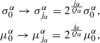
for α ∈ { ∥ , ⊥ }. The jα integer scales of the ψjα wavelets range from 0 to Jα − 1, where Jα is the number of scales. Once Jα is chosen, the value of Qα is fixed so that the wavelet set samples the full extent of the Fourier space. Specifically, when the mother wavelet, centred at μ0α, is dilated up to the largest scale, the resulting ψJα − 1 wavelet is centred at the maximum Fourier scale kα, max, i.e. the Nyquist scale, yielding
 (6)
(6)
To construct the 3D wavelet, we consider the tensor product between the two wavelet sets we previously defined:
 (7)
(7)
where ⊗ is the tensor product. In the following, we use the shorthand notation λ = {j∥, j⊥}, which yields
 (8)
(8)
These wavelets are real in Fourier space and complex in real space.
In this paper, the central frequencies {μ0∥, μ0⊥} of the mother wavelets were chosen to be twice the smallest Fourier scale available, giving {μ0∥, μ0⊥}={0.023 h Mpc−1, 0.028 h Mpc−1}. This choice allows sampling on the largest possible scales, while still enabling the estimation of statistics on non-periodic fields (see Sect. 4.4). We then chose (J∥, J⊥) = (6, 6), corresponding to (Q∥, Q⊥) = (0.90, 0.93), which is close to the commonly used dyadic scaling, resulting in a total of 36 wavelets. Finally, we chose the values {σ0∥, σ0⊥}={0.011 h Mpc−1, 0.015 h Mpc−1} to cover the entire k∥ − k⊥ Fourier plane as uniformly as possible. Fig. 2 shows the resulting wavelet set in this cylindrical Fourier space.
 |
Fig. 2. Different regions in the k∥ vs k⊥ plane characterised by wavelets in the 3D wavelet set. |
This wavelet set applies not only to EoR lightcones but also to all spectroscopic datasets and to any 2+1D field whose third axis represents a different quantity. In this work, we demonstrate its performance on EoR lightcones with limited redshift evolution (Δz ≃ 1); extending the method to fully evolving lightcones with larger Δz is a direction for future work.
3.2. Scattering transform statistics
Scattering transform (ST) statistics are a family of summary statistics. In this work, we consider a simplified version3 of the scattering covariance statistics introduced in Cheng et al. (2023). Consider a 3D lightcone I. Its scattering covariance statistics are defined as
![Mathematical equation: $$ \begin{aligned} C^{p_1,p_2}_{\lambda _1,\lambda _2} = \mathrm{Cov}\big ([I \circledast \Psi _{\lambda _1}]^{p_1},[I \circledast \Psi _{\lambda _2}]^{p_2}\big ), \end{aligned} $$](/articles/aa/full_html/2026/02/aa55896-25/aa55896-25-eq13.gif) (9)
(9)
where ⊛ denotes a convolution and
![Mathematical equation: $$ \begin{aligned}{[z]}^p = {\left\{ \begin{array}{ll} |z|,&\mathrm{if}\; p = 0.\\ z,&\mathrm{if}\; p = 1. \end{array}\right.} \end{aligned} $$](/articles/aa/full_html/2026/02/aa55896-25/aa55896-25-eq14.gif) (10)
(10)
The covariance between two stochastic processes X and Y is defined as Cov(X, Y) = ⟨XY*⟩ − ⟨X⟩⟨Y*⟩, where ⟨⟩ denotes the expected value and * denotes the complex conjugate. In this work, the expected values were estimated using a spatial average.
Using this definition, the three subsets of scattering covariance coefficients are:
 (11)
(11)
 (12)
(12)
 (13)
(13)
In these equations, the condition λ1 ≤ λ2 denotes μj∥, 2∥ ≤ μj∥, 1∥ and μj⊥, 2⊥ ≤ μj⊥, 1⊥, as summarised in Fig. 3. This λ-scale conditioning is explained as follows. For C11, the covariance is zero if λ1 ≠ λ2. Since the spectral supports of different wavelets do not overlap, I ⊛ Ψλ1 and I ⊛ Ψλ2 also have distinct spectral supports and therefore exhibit vanishing covariance, as they are linearly decorrelated4. For C01, convolving I ⊛ Ψλ1 with the first wavelet concentrates the resulting field into a band of scales around λ1. Applying the modulus operator, |I ⊛ Ψλ1|, demodulates the field by re-centering its support towards lower scales (see, e.g. Zhang & Mallat 2019). To obtain a non-vanishing covariance, the secondary wavelet convolution I ⊛ Ψλ2, centred at scales λ2, must now overlap the envelope defined by |I ⊛ Ψλ1|, enforcing λ1 ≤ λ2. For C00, since the covariance is commutative, |I ⊛ Ψλ1| and |I ⊛ Ψλ2| play the same role, so the condition λ1 ≤ λ2 avoids double counting.
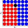 |
Fig. 3. Schematic of the secondary convolution criterion λ1 ≤ λ2, for the 3D wavelets set in the k∥ vs k⊥ plane. The starting wavelet ψλ1 (black) and the second wavelet ψλ2 probe regions such that μj∥, 2∥ ≤ μj∥, 1∥ and μj⊥, 2⊥ ≤ μj⊥, 1⊥. These wavelets, for the example ψλ1, are shown in the highlighted region (red). |
Although the scattering covariances Cp1, p2 capture the non-Gaussian properties of a given lightcone, they also depend on the amplitude of its power spectrum. To correct for this dependence, we normalised the scattering covariances by the C11 of a reference field. In this work, this reference field is the target lightcone and the normalised scattering covariance statistic is denoted  . The normalised scattering covariance statistics are defined as follows:
 (14)
(14)
 (15)
(15)
 (16)
(16)
To further constrain the power spectrum, we used an additional set of C11 coefficients, denoted C11′. These coefficients were computed according to Eq. (11), with a set of wavelets defined as in Sect. 3.1, but with a different number of scales, J′α > Jα. These C11′ coefficients, computed from a larger set of wavelets, used in conjunction with C11, provide an overall improved spectral resolution for power spectrum constraints (Mousset et al. 2024), without increasing the computational complexity for higher-order terms. For these coefficients, we used (J′∥, J′⊥) = (15, 15), corresponding to (Q∥, Q⊥) = (2.53, 2.60).
We concatenated the various ST coefficients to form the set of ST statistics:
 (17)
(17)
The choice of parameters to define the wavelet sets results in 36 coefficients in C11, 225 coefficients in C11′, and 441 coefficients in C01 and C00, for a total of 1143 ST statistics.
4. Generative models
4.1. Maximum entropy microcanonical models
We constructed a maximum entropy model of an EoR lightcone from the scattering covariance statistics on the target lightcone, dt. The new approximate realisations of this lightcone were then sampled using gradient descent (Bruna & Mallat 2018; Allys et al. 2020; Régaldo-Saint Blancard et al. 2023). This gradient descent sampling transforms a white Gaussian distribution into the maximum entropy distribution conditioned on the ST statistics of dt.
The procedure is as follows. The map on which the gradient descent is performed is denoted u. It is initialised with a white noise realisation, u = u0, with a mean and standard deviation matching those of the target lightcone. The optimisation is performed by constraining the scattering transform statistic, ϕ(u), of u with the following loss:
 (18)
(18)
where ∥ ⋅ ∥ is the Euclidean norm and dt is fixed. This gradient descent is performed until the loss converges. The samples,  , from the ST generative model correspond to the map
  obtained at the end of the optimisation, whose ST statistics are close to those of dt. Different
  samples are obtained by initialising the optimisation with different white noise realisations.
4.2. Numerical experiment and statistical validation
To validate the quality of the ST generative models, we compared the statistical properties of the generated lightcones, after performing the inverse quantile transform, with those of the target lightcone, dt. We generated 30 independent synthesised lightcones, denoted  after the inverse quantile transform, each initialised from a different white Gaussian noise realisation. To perform the optimisation, we computed the loss function gradient using automatic differentiation with the L-BFGS-B algorithm (Byrd et al. 1995) (as implemented in PyTorch). We performed the optimisation using 2000 gradient descent iterations, at which point the loss had converged to a plateau after being reduced by approximately ten orders of magnitude. Each optimisation for a single lightcone required two hours on a Nvidia Tesla A100 GPU with 80 GB of memory.
Beyond an initial visual comparison, the statistics considered were the histogram, power spectrum, and Minkowski functionals. In each case, we compared the mean statistics of dt (shown in blue in comparison figures) and of the 30  (shown in green). To assess potential model bias, we compared the difference between these mean statistics and their sample standard deviation, σtoct, between octants of the lightcone5, estimated on the target lightcone, dt. The standard deviation of the St statistics estimator used to construct the generative model is σtoct, since only a volume corresponding to a single octant of the lightcone was used, due to the issue of non-periodic boundary conditions, as explained above. This sampling variance can then simply explain modelling biases of this order.
Additionally, we compared σt and σs, the sample standard deviation across lightcones, estimated from dt and the 30  , respectively. This allowed us to quantify whether the ST generative model reproduces both the mean and sample variance of the statistics. While σs can be estimated directly from the 30
  , σt has to be estimated from dt only. To do this, we approximated the octants of dt as independent, resulting in
  . While this is a rough approximation, which will a priori tend to underestimate σt, since the octant are not independent, it enables a first comparison between σt and σs.
To provide additional comparisons, we also considered the distributions of statistics obtained from 30 Gaussian realisations with the same power spectrum as dt (shown in orange), with their associated lightcone-to-lightcone sample standard deviation, σg, and with the distributions obtained from the complete set of lightcones in the Loreli II database (shown in purple).
A list of the different σ values defined in this section is given in Table 1.
Overview of the defined σ quantities.
4.3. Data conditioning
Prior to the construction of the generative model, the data was conditioned to mitigate several practical issues that could adversely affect the resulting synthesis. This data conditioning ensured that the generative model operated on a well-suited representation of the EoR lightcone, thus improving the fidelity and stability of the subsequent synthesis.
4.3.1. Quantile function
The EoR lightcone is a complex non-Gaussian process, with a highly skewed histogram that is difficult to recover using an ST maximum entropy model. To improve the modelling, we first applied an invertible non-linear transform to the EoR lightcone to obtain a histogram closer to a Gaussian distribution. We then sampled the ST maximum entropy model in this transformed data space, before returning to the original EoR lightcone data space using the inverse non-linear transform.
Such ST modelling based on an invertible non-linear transform has been used in previous studies, for example using a logarithmic pointwise transform before constructing ST generative models (Allys et al. 2020; Régaldo-Saint Blancard et al. 2023; Mousset et al. 2024). This approach is particularly useful for modelling processes with complex histograms, such as those with only non-negative values, including the matter density of large-scale structures in the Universe. The general idea of transforming a process into another one that is better approximated is also used when constructing lognormal models for processes whose logarithm is expected to be much better described by a Gaussian model than the process itself. Lognormal models are used, for example, to describe the thermal emission of Galactic molecular clouds (Miville-Deschênes et al. 2007; Levrier et al. 2018).
In this work, we used a quantile transformation to map the histogram of the target lightcone to a normal distribution (Mark Beasley & Erickson 2009; McCullagh & Tresoldi 2020). To do this, we first estimated the global empirical cumulative distribution function (CDF)  of the field for the entire (δν ∼ 14 MHz) lightcone. We then computed the corresponding percentile p for each data point d(r) in the lightcone,
 (19)
(19)
Next, this percentile p was passed into the inverse of the standard normal CDF (also known as the quantile function) to obtain
 (20)
(20)
This procedure produces a set of  values that follow a normal distribution, replacing the original skewed distribution while preserving the ordering of the original data points.
In this work, the quantiles for the transform were estimated from all data points within the target lightcone. The choice of the number of quantiles corresponds to a standard bias-variance trade-off: too few quantiles result in a poor representation of the data distribution, while too many can introduce overfitting and unnecessary computational overhead. We empirically find that 10 000 quantiles provide a good balance. Given that the target lightcone contains approximately 106 pixels, using 10 000 quantiles corresponds to approximately 300 pixels per quantile. This quantile-to-pixel ratio is sufficient to accurately represent the low density tail of the distribution without incurring needless computational cost.
It should be noted that the quantile transform is not a pointwise operator but is instead applied by analysing the entire lightcone simultaneously. Although this transform efficiently models complex histograms, any modelling error in the transformed data space can cause significant instabilities in the inverse transform. In particular, the significant effect of large scales on the histogram, which are difficult to model statistically from a small amount of data, can make it difficult to use such a transform.
4.3.2. Treatment of unconstrained scales
The generative model in this work does not constrain two limiting ranges of scales. The first unconstrained range, denoted κlow, corresponds to the largest scales, which have Fourier mode wavenumbers smaller than the mother wavelet’s wavenumber, μ0. The second unconstrained range, denoted κhigh, corresponds to the smallest scales, which have Fourier modes beyond the Nyquist frequency.
Since we first constructed the ST generative model on the quantile-transformed data before applying the inverse quantile transform, these unconstrained scales can significantly affect the final synthesised lightcone because the transform is the non-linear and non-local. To mitigate their impact, we handled them explicitly, as described below:
-
The κlow scales were replaced with the corresponding modes from the target lightcone in the transformed data space. This substitution occurred prior to the gradient descent optimisation, ensuring that these large-scale modes were included in the initial conditions. This was necessary because, if left unconstrained, these scales would influence the global inverse quantile transform. Since these scales are not characterised by the ST statistics, they do not directly influence the generation of the remaining scales during the optimisation process.
-
The κhigh scales in the target lightcone were filtered prior to the quantile transform, both when constructing the generative model and when comparing with the synthesised maps. Although the non-linearity of the quantile transform introduces some beyond-Nyquist scales after the histogram transform, their effect on the inverse histogram transform after modelling is negligible.
In principle, our framework can be run without re-inserting the modes with k < klow from the target lightcone. In this case, these modes remain unconstrained by the optimisation process. The generative model still visually reproduces the target lightcone and accurately matches the scattering statistics on intermediate and small scales. However, the largest scales show biased power, with deviations at k ≲ κlow comparable to, although generally within, the sample variance of the target lightcone. We also experimented with replacing the modes with Gaussian realisations matched to the target power spectrum. However, because the quantile transform is a global, non-linear mapping, the large-scale modes strongly influence the histogram. Consequently, even modest higher-order mismatches propagate into systematic biases at low k after the inverse transform. A more physical alternative would be to source these large-scale modes from a dedicated low-resolution EoR simulation. However, consistently coupling them to the high-resolution, quantile-transformed small scales is non-trivial, and we leave this as an interesting direction for future work.
4.4. Non-periodic boundary conditions
Simulations of the EoR lightcone have non-periodic boundaries, in particular because of the redshift evolution along the line of sight. However, since we compute convolutions by products in Fourier space, these are inherently periodic. To avoid taking boundary discontinuities into account when estimating the ST statistics, the empirical covariances were computed only over a central smaller cubic volume of the data6. This is achieved by cropping the edges of the wavelet convolved fields, so that all pixels over which the average is computed are sufficiently separated from the boundaries. To verify this, the cropped band sizes are matched to the maximum sizes characterised by the wavelets, which are determined by the mother wavelet scale  . Specifically, we removed a width at each end of each axis equal to half the mother wavelet scale on that axis, yielding an average over a volume of (61, 61, 87) pixels.
Note that while the statistics of the target lightcones, estimated on dt and used to constrain the generative model, were computed taking into account the non-periodic boundary conditions as described above, the samples generated by this generative model are full lightcones with periodic boundary conditions. To achieve this, their initial conditions were white noise defined over the entire (128, 128, 170) pixels data cube, and their statistics were computed using period convolutions and averages over the entire cube. We performed these syntheses by comparing the two types of ST statistics estimators, with and without periodic boundary conditions, in Eq. (18). As a side effect, the statistics used to construct the generative models were estimated from only about one eighth of the target lightcone volume, leading to a higher sampling variance.
5. Validation of the generative models
5.1. Visual validation
A first test of synthesis quality is to visually compare three realisations,  , of a synthesised lightcone with the target lightcone, dt. The xy-slice comparison (Fig. 4) shows that these three realisations are visually similar to dt. The target lightcone contains several distinctive features, such as strongly localised absorbing (negative) regions and ionised (near-zero) regions, which serve as touchstones that the synthesised lightcones successfully capture. Fig. 5 shows that the synthesised lightcones again reproduce the different phases of the field (emission, absorption, and ionised) and the elongated structures characteristic of the redshift axis. However, the generated samples appear to exhibit a greater diversity in the distribution of ionised regions, although a quantitative assessment is difficult from a single dt lightcone.
 |
Fig. 4. Comparison of a given xy-slice (single frequency channel in the lightcone), for the target EoR lightcone and three synthesised lightcones generated using the 3D scattering transforms with the inverse quantile transform applied. The synthesised lightcones visually reproduce the target lightcone well. |
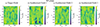 |
Fig. 5. Same as Fig. 4, but for a given xz-slice (with z representing the redshift domain) for the target EoR lightcone and three synthesised lightcones. As in Fig. 4, the target lightcone is visually well reproduced by the synthesised lightcones. |
5.2. Histogram
Fig. 6 compares normalised histograms (i.e. the estimated probability density functions) of the target (blue) and synthesised (green) lightcones. The target lightcone exhibits a non-symmetric, left-skewed tail distribution, a clear, highly non-Gaussian signature, which the synthesised lightcones accurately reproduce over approximately four orders of magnitude, down to δTb = −7 mK. The bottom plot of Fig. 6 shows that the difference between these histograms, normalised by σtoct, mostly lies between −1 and 1, consistent with the estimation variance of the target ST statistics. The top plot of Fig. 6 shows that σs, the lightcone-to-lightcone standard deviation for the synthesised maps, is of the same order as the bin-to-bin variability of the histogram estimated on dt, indicating that this variance is also well reproduced. The standard deviation, σt, is not shown in the top plot, as the sample variability is already apparent due to the fine binning.
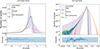 |
Fig. 6. Linear- and log-scale histograms of the target EoR lightcone and a synthesised lightcone after the inverse quantile transform. The histogram of the synthesised lightcone, showing the mean of 30 realisations and their standard deviation (shaded region), recovers the histogram of the target lightcone well, including its skewness. |
We used negative brightness temperature values (δTb) as a proxy for ionised pixels to infer the neutral fraction of the lightcone. The neutral fraction of the target lightcone is 0.617. The mean neutral fraction of the 30 generated lightcones is 0.624 ± 0.001, indicating that the generative model can recover the target lightcone’s neutral fraction to 1% accuracy.
5.3. Power spectrum
Four power spectra were used to compare the target and synthesised lightcones: the 3D isotropic power spectrum; the 2D isotropic power spectrum on the xy or xz planes; and the cylindrically averaged power spectrum. Although the cylindrically averaged power spectrum is sometimes referred to as the 2D power spectrum, here it specifically refers to the power spectrum estimated on actual 2D fields: each 2D xy or xz slice, averaged over the z or y axis, respectively. We refer the reader to Appendix A for more details. Comparisons with Gaussian realisations are not included in this section, as these have the same power spectrum as the target lightcone.
Figure 7a compares the 3D isotropic power spectrum of the target lightcone and that of the synthesised lightcones. The power spectrum of the synthesised lightcones closely follows that of the target lightcone, remaining within ±σs on most scales. Although estimating σtoct for the power spectrum is challenging, due to the differing numbers of modes per bin for different data sizes, the averaged 3D power spectrum of the synthesised lightcones reproduces that of dt within 25% across the range 0.1 and 1 h Mpc−1. Figures 7b and 7c show similar results for the 2D power spectra in the xy− and xz− planes. In these cases, a visible bias appears at the smallest scales, with syntheses reproducing the dt power spectra to within 15% on average across 0.2−1 h Mpc−1. The shape of the power spectra in Figure 7c results from discretisation effects introduced by the binning scheme in the cylindrical Fourier plane, which imposes a structure on the spectra.
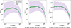 |
Fig. 7. Comparison between the target and synthesised lightcones after the inverse quantile transform, showing power spectra across different dimensions. (a) Spherically-averaged 3D power spectrum. (b) 2D power spectrum estimated on xy-planes. (c) 2D power spectrum estimated on xz-planes. In all cases the power spectra of the synthesised lightcones reproduce the largest scales well, with increasing deviations at smaller scales. |
Fig. 8 compares of the cylindrically averaged power spectra, where the synthesised lightcones are represented by the mean spectrum of the 30 realisations. The right panel shows the ratio of the target lightcone’s cylindrically averaged power spectrum to that of the mean of the synthesised lightcones. Overall, the cylindrical power spectra are well reproduced, but Fig. 8c highlights large ratio values at high k∥ and k⊥. These correspond to the bias we see at high k in the power spectrum comparison in Fig. 7, close to Nyquist frequencies. Apart from the bias observed at high k modes, the cylindrical power spectra of the synthesised lightcones remain within  of the variance across the 30 realisations at all other scales.
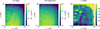 |
Fig. 8. Comparisons of the cylindrically averaged power spectrum of the target lightcone (left) and synthesised lightcones (middle) after the inverse quantile transform. The ratio between the two cylindrically averaged power spectra is also shown (right), with the power spectra of the synthesised lightcones reproducing that of the target lightcone within 25%, on most scales below k∥ = 0.3 h Mpc−1. |
The high-k bias in the power spectra of the synthesised lightcones, particularly along the z domain, is not a limitation of the C11 and C11′ power spectrum constraints. Prior to the application of the inverse quantile transform, power spectra recover well at these scales, with only small bias. However, this bias increases significantly when the transform is subsequently applied. This likely arises because non-Gaussian structures, i.e. the statistical dependence between the different scales, are not properly reproduced at small scales. In this scenario, the highly non-linear inverse histogram transform could introduce such a bias. To address this issue, the C11 and C11′ power spectrum constraints could be added after this transform, at the expense of additional computational time.
5.4. Minkowski functionals
Finally, we compared the Minkowski functionals (MFs) of the target and the synthesised lightcones, which were computed using the Minkowski functionals function of the QuantImPy Python package (Boelens & Tchelepi 2021). As with the 2D isotropic power spectrum, we computed the 2D MFs on the xy and xz planes, which were then averaged over the z or y axes, respectively. The three MFs are M0, M1, and M2 (Mecke et al. 1994; Schmalzing & Buchert 1997). These 2D MFs were computed by progressively increasing a threshold value and evaluating the properties of the regions above this threshold: total area (M0), perimeter (M1), and genus (M2), which provides insight into the connectivity and complexity of ionised structures.
To address the non-periodic boundary conditions of dt, the MFs were computed on the xy or xz planes after applying a complete symmetric padding to restore periodicity without significantly altering the underlying data (this results in some sharp edges at the initial boundary position). We also applied this symmetric padding when estimating the MFs of the syntheses, even though they have periodic boundary conditions, to ensure the best possible comparison.
Figures 9 and 10, show the MFs in the xy and xz planes, respectively. Since the lightcone-to-lightcone standard deviations (σt, σs, and σg) are very small, they are multiplied by a factor of 10 in the plots. These plots show that all three MFs of the synthesised lightcones closely resemble those of dt in both xy and xz planes. This indicates that the ST generative models effectively reproduce the morphological features of the data. However, while the differences between these mean statistics mostly remain within ±σtoct for the xz-MFs, this is not entirely the case for the xy-MFs, for which clear deviations are particularly visible for M2. We interpret this as the first limitation of the ST generative model, arising from its difficulty in reproducing the sharp, high-contrast, and highly textured circular features present in the target lightcone (see Fig. 4). Overall, for both xy and xz cases, the M0, M1, and M2 statistics are reproduced within 1%, 10%, and 15%, respectively.
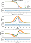 |
Fig. 9. Comparison of the Minkowski functionals applied to each frequency channel of the lightcone between the synthesised lightcones (after the inverse quantile transform) and the target lightcone. The mean Minkowski functionals across the lightcone are shown, with shaded regions indicating their standard deviation. From the bottom panel, M0 and M1 of the synthesised lightcones recover the target lightcone’s Minkowski functionals well, lying within the octant variance, σtoct, and reproducing its morphology. The M2 of the synthesised lightcone follows that of the target lightcone and lies within ±2.5σtoct. |
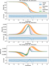 |
Fig. 10. Same as Fig. 9, but for the xz-plane. The synthesised lightcones reproduce the functionals of the xz-plane, recovering the morphology of the evolving lightcone. These functionals lie within the octant variance, σtoct, of the target lightcone. |
Notably, the synthesised data have a lightcone-to-lightcone standard deviation, σs, which is a few times smaller than the standard deviation σt estimated from dt. In contrast, Gaussian models exhibit considerably larger variance. This could indicate a second limitation of ST generative models. However, care should be taken when interpreting this result, as estimating σt from σtoct could lead to a substantial underestimation of this variance, which could be larger between lightcones than within them.
6. Conclusions
The 21 cm signal from the Epoch of Reionisation (EoR) is observed by radio interferometers as a lightcone that includes a 2D sky plane and a 1D redshift domain that captures the signal’s evolution. These observations are contaminated by foregrounds that are several orders of magnitude stronger than the EoR signal, which the instruments are designed to detect. Recently developed component separation methods rely on maximum entropy generative models based on scattering transforms. In this work, we explored the feasibility of generative models of EoR lightcones built from 3D scattering transforms.
We constructed the 3D scattering transforms from a wavelet set obtained by taking the tensor product between a 1D wavelet set defined in kz and a 2D wavelet set defined in the kx − ky plane. We demonstrated the performance of these generative models by applying them to a single simulated EoR lightcone from the LoReLi II database. We validated the generative model by comparing several realisations of the synthesised lightcone with the original target lightcone, using independent statistical estimators, including histograms, 3D and 2D power spectra, cylindrically averaged power spectra, and Minkowski functionals.
The results demonstrate that the synthesised lightcones accurately reproduce the key non-Gaussian properties and morphology of the target lightcone, including its characteristic skewed histogram, redshift-dependent structures, and morphological complexity, as probed by the Minkowski functionals. These statistics were well reproduced within the expected sample variance estimated from the data.
Beyond the overall validation, several limitations were identified:
-
The synthesised lightcones reproduce the target power spectra over a wide range of scales, but clear biases appear at high-k (small scales), particularly along the redshift axis. This indicates limitations of the generative model when combined with the inverse quantile transformation. However, this could be mitigated by additional post-inverse corrections or by refining the treatment of scales not constrained by the scattering transforms.
-
The synthesised lightcone Minkowski functionals do not fully reproduce the M2 of the target lightcone. This suggests that the generative model struggles to produce sharp, high-contrast circular features in the target lightcone, such as ionised regions. More sophisticated scattering transform representation, such as complete scattering spectra statistics (Cheng et al. 2023), could address this, but at an additional computational cost.
-
The synthesised lightcones display diverse realisations, but the variance between them may be slightly overestimated compared to the variance estimated over the octants of the target lightcone. More simulated data would be required to adequately estimate this lightcone-to-lightcone variability.
Overall, this study provides the first proof-of-concept for applying 3D scattering transform-based generative models to EoR lightcones. These results pave the way for the development of a statistical component separation method using 3D scattering transform statistics to separate the EoR signal from a realistic forward-modelled lightcone with foregrounds and noise.
Although our tests focus on EoR lightcones with a modest redshift extent, the approach is generally applicable to other spectroscopic datasets and 3D fields in which the third axis represents a different quantity. A natural next step is to apply the method to full lightcones with stronger redshift evolution across the volume.
Acknowledgments
The post-doctoral contract of Ian Hothi was funded by Sorbonne Université in the framework of the Initiative Physique des Infinis (IDEX SUPER) and through the overheads of Edith Falgarone’s MIST ERC. We would like to thank Florent Mertens and Adélie Gorce for their useful discussions and input. The Loreli project was provided with computer and storage resources by GENCI at TGCC thanks to the grants 2022-A0130413759 and 2023-A0150413759 on the supercomputer Joliot Curie’s ROME partition. This work was granted access to the HPC resources of MesoPSL financed by the Region Ile de France and the project Equip@Meso (reference ANR-10-EQPX-29-01) of the programme Investissements d’Avenir supervised by the Agence Nationale pour la Recherche. This research made use of astropy, a community-developed core Python package for astronomy (Astropy Collaboration 2018); scipy, a Python-based ecosystem of open-source software for mathematics, science, and engineering (Virtanen et al. 2020) – including numpy (Walt et al. 2011); matplotlib, a Python library for publication quality graphics (Hunter 2007).
References
- Allys, E., Levrier, F., Zhang, S., et al. 2019, A&A, 629, A115 [NASA ADS] [CrossRef] [EDP Sciences] [Google Scholar]
- Allys, E., Marchand, T., Cardoso, J. F., et al. 2020, Phys. Rev. D, 102, 103506 [Google Scholar]
- Astropy Collaboration (Price-Whelan, A. M., et al.) 2018, AJ, 156, 123 [Google Scholar]
- Auclair, C., Allys, E., Boulanger, F., et al. 2024, A&A, 681, A1 [NASA ADS] [CrossRef] [EDP Sciences] [Google Scholar]
- Becker, G. D., Bolton, J. S., Madau, P., et al. 2015, MNRAS, 447, 3402 [Google Scholar]
- Blamart, M., & Liu, A. 2025, ArXiv e-prints [arXiv:2505.09674] [Google Scholar]
- Boelens, A. M., & Tchelepi, H. A. 2021, SoftwareX, 16, 100823 [Google Scholar]
- Bosman, S. E. I., Fan, X., Jiang, L., et al. 2018, MNRAS, 479, 1055 [Google Scholar]
- Bruna, J., & Mallat, S. 2012, ArXiv e-prints [arXiv:1203.1513] [Google Scholar]
- Bruna, J., & Mallat, S. 2018, ArXiv e-prints [arXiv:1801.02013] [Google Scholar]
- Byrd, R. H., Lu, P., Nocedal, J., & Zhu, C. 1995, SIAM J. Sci. Comput., 16, 1190 [Google Scholar]
- Campeti, P., Delouis, J.-M., Pagano, L., et al. 2025, A&A, 700, A136 [NASA ADS] [CrossRef] [EDP Sciences] [Google Scholar]
- Cheng, S., Ting, Y.-S., Ménard, B., & Bruna, J. 2020, MNRAS, 499, 5902 [Google Scholar]
- Cheng, S., Morel, R., Allys, E., Ménard, B., & Mallat, S. 2023, ArXiv e-prints [arXiv:2306.17210] [Google Scholar]
- Datta, A., Bowman, J. D., & Carilli, C. L. 2010, ApJ, 724, 526 [NASA ADS] [CrossRef] [Google Scholar]
- Delouis, J. M., Allys, E., Gauvrit, E., & Boulanger, F. 2022, A&A, 668, A122 [NASA ADS] [CrossRef] [EDP Sciences] [Google Scholar]
- Eickenberg, M., Allys, E., Moradinezhad Dizgah, A., et al. 2022, ArXiv e-prints [arXiv:2204.07646] [Google Scholar]
- Fan, X., Strauss, M. A., Becker, R. H., et al. 2006, AJ, 132, 117 [NASA ADS] [CrossRef] [Google Scholar]
- Gorce, A., Douspis, M., Aghanim, N., & Langer, M. 2018, A&A, 616, A113 [EDP Sciences] [Google Scholar]
- Gorce, A., Douspis, M., & Salvati, L. 2022, A&A, 662, A122 [NASA ADS] [CrossRef] [EDP Sciences] [Google Scholar]
- Greig, B., Ting, Y.-S., & Kaurov, A. A. 2022, MNRAS, 513, 1719 [NASA ADS] [CrossRef] [Google Scholar]
- Hothi, I., Chapman, E., Pritchard, J. R., et al. 2021, MNRAS, 500, 2264 [Google Scholar]
- Hothi, I., Allys, E., Semelin, B., & Boulanger, F. 2024, A&A, 686, A212 [NASA ADS] [CrossRef] [EDP Sciences] [Google Scholar]
- Hunter, J. D. 2007, Comput. Sci. Eng., 9, 90 [NASA ADS] [CrossRef] [Google Scholar]
- Jelić, V., Zaroubi, S., Labropoulos, P., et al. 2008, MNRAS, 389, 1319 [CrossRef] [Google Scholar]
- Kumar, N. A., Çalışkan, M., Hotinli, S. C., et al. 2025, ArXiv e-prints [arXiv:2506.11188] [Google Scholar]
- Lei, M., & Clark, S. 2023, ApJ, 947, 74 [NASA ADS] [CrossRef] [Google Scholar]
- Levrier, F., Neveu, J., Falgarone, E., et al. 2018, A&A, 614, A124 [NASA ADS] [CrossRef] [EDP Sciences] [Google Scholar]
- Liu, A., Parsons, A. R., & Trott, C. M. 2014, Phys. Rev. D, 90, 023018 [NASA ADS] [CrossRef] [Google Scholar]
- MacCrann, N., Qu, F. J., Namikawa, T., et al. 2024, MNRAS, 532, 4247 [Google Scholar]
- Mallat, S. 2011, ArXiv e-prints [arXiv:1101.2286] [Google Scholar]
- Mark Beasley, T., & Erickson, S. 2009, Behav. Genet., 39, 580 [Google Scholar]
- McCullagh, P., & Tresoldi, M. F. 2020, ArXiv e-prints [arXiv:2001.03709] [Google Scholar]
- Mecke, K. R., Buchert, T., & Wagner, H. 1994, A&A, 288, 697 [NASA ADS] [Google Scholar]
- Meriot, R., & Semelin, B. 2024, A&A, 683, A24 [NASA ADS] [CrossRef] [EDP Sciences] [Google Scholar]
- Meriot, R., Semelin, B., & Cornu, D. 2025, A&A, 698, A80 [NASA ADS] [CrossRef] [EDP Sciences] [Google Scholar]
- Miville-Deschênes, M.-A., Lagache, G., Boulanger, F., & Puget, J.-L. 2007, A&A, 469, 595 [NASA ADS] [CrossRef] [EDP Sciences] [Google Scholar]
- Mousset, L., Allys, E., Price, M. A., et al. 2024, A&A, 691, A269 [NASA ADS] [CrossRef] [EDP Sciences] [Google Scholar]
- Munshi, S., Mertens, F. G., Koopmans, L. V. E., et al. 2025, A&A, 693, A276 [NASA ADS] [CrossRef] [EDP Sciences] [Google Scholar]
- Murray, S. G., & Trott, C. M. 2018, ApJ, 869, 25 [NASA ADS] [CrossRef] [Google Scholar]
- Planck Collaboration XLVII. 2016, A&A, 596, A108 [NASA ADS] [CrossRef] [EDP Sciences] [Google Scholar]
- Prelogović, D., & Mesinger, A. 2024, A&A, 688, A199 [NASA ADS] [CrossRef] [EDP Sciences] [Google Scholar]
- Qin, Y., Mesinger, A., Bosman, S. E. I., & Viel, M. 2021, MNRAS, 506, 2390 [NASA ADS] [CrossRef] [Google Scholar]
- Regaldo-Saint Blancard, B., Levrier, F., Allys, E., Bellomi, E., & Boulanger, F. 2020, A&A, 642, A217 [EDP Sciences] [Google Scholar]
- Regaldo-Saint Blancard, B., Allys, E., Boulanger, F., Levrier, F., & Jeffrey, N. 2021, A&A, 649, L18 [NASA ADS] [CrossRef] [EDP Sciences] [Google Scholar]
- Régaldo-Saint Blancard, B., Allys, E., Auclair, C., et al. 2023, ApJ, 943, 9 [CrossRef] [Google Scholar]
- Régaldo-Saint Blancard, B., Hahn, C., Ho, S., et al. 2024, Phys. Rev. D, 109, 083535 [CrossRef] [Google Scholar]
- Reichardt, C. L., Patil, S., Ade, P. A. R., et al. 2021, ApJ, 908, 199 [NASA ADS] [CrossRef] [Google Scholar]
- Schmalzing, J., & Buchert, T. 1997, ApJ, 482, L1 [NASA ADS] [CrossRef] [Google Scholar]
- Semelin, B., Combes, F., & Baek, S. 2007, A&A, 474, 365 [NASA ADS] [CrossRef] [EDP Sciences] [Google Scholar]
- Semelin, B., Eames, E., Bolgar, F., & Caillat, M. 2017, MNRAS, 472, 4508 [NASA ADS] [CrossRef] [Google Scholar]
- Shaver, P. A., Windhorst, R. A., Madau, P., & de Bruyn, A. G. 1999, A&A, 345, 380 [Google Scholar]
- Shimabukuro, H., Yoshiura, S., Takahashi, K., Yokoyama, S., & Ichiki, K. 2017, MNRAS, 468, 1542 [NASA ADS] [CrossRef] [Google Scholar]
- Shimabukuro, H., Xu, Y., & Shao, Y. 2025, Phys. Rev. D, 112, 063557 [Google Scholar]
- Tiwari, H., Shaw, A. K., Majumdar, S., Kamran, M., & Choudhury, M. 2022, JCAP, 2022, 045 [Google Scholar]
- Valogiannis, G., & Dvorkin, C. 2022, Phys. Rev. D, 105, 103534 [Google Scholar]
- Vedantham, H., Udaya Shankar, N., & Subrahmanyan, R. 2012, ApJ, 745, 176 [NASA ADS] [CrossRef] [Google Scholar]
- Virtanen, P., Gommers, R., Oliphant, T. E., et al. 2020, Nat. Meth., 17, 261 [Google Scholar]
- Walt, S. V. D., Colbert, S. C., & Varoquaux, G. 2011, Comput. Sci. Eng., 13, 22 [Google Scholar]
- Watkinson, C. A., Greig, B., & Mesinger, A. 2022, MNRAS, 510, 3838 [CrossRef] [Google Scholar]
- Zhang, S., & Mallat, S. 2019, ArXiv e-prints [arXiv:1911.10017] [Google Scholar]
- Zhao, X., Ting, Y.-S., Diao, K., & Mao, Y. 2023, MNRAS, 526, 1699 [NASA ADS] [CrossRef] [Google Scholar]
- Zhao, X., Mao, Y., Zuo, S., & Wandelt, B. D. 2024, ApJ, 973, 41 [Google Scholar]
The z-domain, or line of sight, is denoted by ∥, and the xy-plane, the perpendicular sky domain, denoted by ⊥.
However, foregrounds can leak across the wedge line (Murray & Trott 2018).
Compared with the statistics defined in Cheng et al. (2023), no second convolution is explicitly performed. These statistics can also be viewed as a compact form of the wavelet phase harmonics statistics introduced in Allys et al. (2020), where only p = 0 and p = 1 phase harmonics are considered, and no translations are performed prior to covariance estimation.
This can be shown using Plancherel’s Theorem.
To create octants, the data cube was divided into eight equal sub-volumes, of dimension (64, 64, 85) pixels. These octants have approximately the same volume as the region used to estimate the ST statistics due to non-periodic boundary conditions.
In practice a rectangular parallelepiped, as the original lightcone.
Appendix A: Power spectrum binning
The dimensionless power spectrum of the 21cm brightness temperature I is defined as
 (A.1)
(A.1)
where k (=kx, ky, kz) is the wavenumber and Wi(k) is the spectral window function that defines the ith bin. We choose the spectral window function to be a top-hat function defined as,
![Mathematical equation: $$ \begin{aligned} W_i(\boldsymbol{k}) = {\left\{ \begin{array}{ll} 1,&\mathrm{if}\; {\boldsymbol{k}}_i \le \boldsymbol{k} < {\boldsymbol{k}}_{i+1}\\ [1mm] 0,&\mathrm{otherwise} \end{array}\right.} \end{aligned} $$](/articles/aa/full_html/2026/02/aa55896-25/aa55896-25-eq42.gif) (A.2)
(A.2)
where ki defines the lower wavenumber limit of the ith bin. These window functions are assumed to be isotropic, so W(k) = W(k) with k = |k|. For the 3D power spectrum Ak = k3 and for the 2D power spectrum Ak = k2.
Before estimating the power spectrum, it is essential to account for the non-periodic boundary conditions of the target lightcone. We address this by applying a Blackman-Harris window function to the data prior to the Fourier transform. Specifically, for the 3D power spectrum, we apply the 1D Blackman-Harris window function separately along each axis of the 3D lightcone. Similarly, for the 2D power spectrum, this window is applied independently along each axis of the respective 2D field. This windowing procedure is applied consistently to both the target dt and synthesised  lightcones; although the
  have periodic boundary conditions, this application ensures consistent treatment of boundary effects.
In addition, we also restrict the power spectra estimation to the range of scales that are well constrained by the generative model, so that the range of k modes that are binned is limited to κlow ≤ k ≤ κhigh (see Section 4.3.2 for definitions).
The dimensionless cylindrically averaged power spectrum, which bins the k∥ and k⊥ domains separately, is defined as
 (A.3)
(A.3)
where Ak = k3, for  . We again assume an isotropic top-hat function, Wi(k∥, k⊥), for k∥ = |k∥| and k⊥ = |k⊥|, yielding
![Mathematical equation: $$ \begin{aligned} W_i(k_\parallel , k_\perp ) = {\left\{ \begin{array}{ll} 1,&\mathrm{if}\; k_{\parallel ,i} \le k_\parallel < k_{\parallel ,i+1} \; \& \;k_{\perp ,i} \le k_\perp < k_{\perp ,i+1}\\ [1mm] 0,&\mathrm{otherwise} \end{array}\right.} \end{aligned} $$](/articles/aa/full_html/2026/02/aa55896-25/aa55896-25-eq47.gif) (A.4)
(A.4)
where k∥, i defines the lower wavenumber limit of the ith along the k∥ domain, and k⊥, i defines the lower wavenumber limit of the ith along the k⊥ domain.
All Tables
All Figures
|
Fig. 1. Schematic of the cylindrically-averaged power spectrum of an observed EoR lightcone, with the three distinct regions highlighted. |
| In the text | |
|
Fig. 2. Different regions in the k∥ vs k⊥ plane characterised by wavelets in the 3D wavelet set. |
| In the text | |
|
Fig. 3. Schematic of the secondary convolution criterion λ1 ≤ λ2, for the 3D wavelets set in the k∥ vs k⊥ plane. The starting wavelet ψλ1 (black) and the second wavelet ψλ2 probe regions such that μj∥, 2∥ ≤ μj∥, 1∥ and μj⊥, 2⊥ ≤ μj⊥, 1⊥. These wavelets, for the example ψλ1, are shown in the highlighted region (red). |
| In the text | |
|
Fig. 4. Comparison of a given xy-slice (single frequency channel in the lightcone), for the target EoR lightcone and three synthesised lightcones generated using the 3D scattering transforms with the inverse quantile transform applied. The synthesised lightcones visually reproduce the target lightcone well. |
| In the text | |
|
Fig. 5. Same as Fig. 4, but for a given xz-slice (with z representing the redshift domain) for the target EoR lightcone and three synthesised lightcones. As in Fig. 4, the target lightcone is visually well reproduced by the synthesised lightcones. |
| In the text | |
|
Fig. 6. Linear- and log-scale histograms of the target EoR lightcone and a synthesised lightcone after the inverse quantile transform. The histogram of the synthesised lightcone, showing the mean of 30 realisations and their standard deviation (shaded region), recovers the histogram of the target lightcone well, including its skewness. |
| In the text | |
|
Fig. 7. Comparison between the target and synthesised lightcones after the inverse quantile transform, showing power spectra across different dimensions. (a) Spherically-averaged 3D power spectrum. (b) 2D power spectrum estimated on xy-planes. (c) 2D power spectrum estimated on xz-planes. In all cases the power spectra of the synthesised lightcones reproduce the largest scales well, with increasing deviations at smaller scales. |
| In the text | |
|
Fig. 8. Comparisons of the cylindrically averaged power spectrum of the target lightcone (left) and synthesised lightcones (middle) after the inverse quantile transform. The ratio between the two cylindrically averaged power spectra is also shown (right), with the power spectra of the synthesised lightcones reproducing that of the target lightcone within 25%, on most scales below k∥ = 0.3 h Mpc−1. |
| In the text | |
|
Fig. 9. Comparison of the Minkowski functionals applied to each frequency channel of the lightcone between the synthesised lightcones (after the inverse quantile transform) and the target lightcone. The mean Minkowski functionals across the lightcone are shown, with shaded regions indicating their standard deviation. From the bottom panel, M0 and M1 of the synthesised lightcones recover the target lightcone’s Minkowski functionals well, lying within the octant variance, σtoct, and reproducing its morphology. The M2 of the synthesised lightcone follows that of the target lightcone and lies within ±2.5σtoct. |
| In the text | |
|
Fig. 10. Same as Fig. 9, but for the xz-plane. The synthesised lightcones reproduce the functionals of the xz-plane, recovering the morphology of the evolving lightcone. These functionals lie within the octant variance, σtoct, of the target lightcone. |
| In the text | |
Current usage metrics show cumulative count of Article Views (full-text article views including HTML views, PDF and ePub downloads, according to the available data) and Abstracts Views on Vision4Press platform.
Data correspond to usage on the plateform after 2015. The current usage metrics is available 48-96 hours after online publication and is updated daily on week days.
Initial download of the metrics may take a while.