| Issue |
A&A
Volume 706, February 2026
|
|
|---|---|---|
| Article Number | A142 | |
| Number of page(s) | 9 | |
| Section | Astrophysical processes | |
| DOI | https://doi.org/10.1051/0004-6361/202556311 | |
| Published online | 05 February 2026 | |
Clues to the photosphere emission origin of gamma-ray burst polarization
1
School of Science, Guangxi University of Science and Technology Liuzhou Guangxi 545006, People’s Republic of China
2
Yunnan Observatories, Chinese Academy of Sciences Kunming, People’s Republic of China
★ Corresponding author: This email address is being protected from spambots. You need JavaScript enabled to view it.
Received:
8
July
2025
Accepted:
12
December
2025
Abstract
Context. Despite more than half a century of research, the dominant radiation mechanism of gamma-ray burst (GRB) prompt emission remains unsolved. Some progress has been made through the analyses of the observational spectra of Swift/BAT, Konus/Wind, and Fermi/GBM, as well as the spectra of the photosphere or synchrotron models, but it is still insufficient to pin down the answer.
Aims. Combining the spectral and polarization observations, we seek new criteria for model evaluation.
Methods. We thoughtfully investigated the polarization samples of POLAR and AstroSAT, combining the light curve, spectral, and polarization parameters.
Results. The power-law shape of the X-ray afterglows, the T90 ∝ (Liso)−0.5 correlation, and the hard low-energy spectral index α are revealed, thus supporting the photosphere origin. Furthermore, we discovered the positive correlation of α and the polarization degree (PD), which can be consistently explained by the photosphere polarization scenario involving the jet asymmetry from a moderate viewing angle of θv = 0.015.
Key words: polarization / radiation mechanisms: thermal
© The Authors 2026
 Open Access article, published by EDP Sciences, under the terms of the Creative Commons Attribution License (https://creativecommons.org/licenses/by/4.0), which permits unrestricted use, distribution, and reproduction in any medium, provided the original work is properly cited.
This article is published in open access under the Subscribe to Open model. This email address is being protected from spambots. You need JavaScript enabled to view it. to support open access publication.
1. Introduction
Gamma-ray bursts (GRBs) are the strongest explosions in our Universe. Several thousand timing and spectral observations have been accumulated since its first discovery in the late 1960s. Based on these, the ultra-relativistic jet is believed to be responsible for producing GRBs. However, the jet properties (especially the structure and composition) are still not well known (Mészáros 2002; Zhang 2020). With additional observation information, for example the azimuthal scattering angle distribution of the incoming photons (standing for the polarization), these properties could be better constrained. The azimuthal scattering angle is defined as the angle between a fixed X-axis (in the X − Y plane perpendicular to the moving direction of the incoming photon) and the projection of the momentum vector of the outgoing photon (after Compton scattering in the first detector segment) onto the X − Y plane. To obtain this azimuthal angle, one should be able to detect the outgoing photon interacting with a second detector segment, through a second Compton scattering or photo-absorption. The azimuthal scattering angle is then deduced from the position of these two detector segments. Finally, a histogram of the azimuthal scattering angle (namely the azimuthal scattering angle distribution) for all the photons performing more than two interactions is achieved, referred to as a modulation curve. The amplitude of this curve represents the polarization degree and its phase is related to the polarization angle (PA). Up until now, only about two dozen polarization detections have been reported (Coburn & Boggs 2003; Yonetoku et al. 2011, 2012; Covino & Gotz 2016; Chattopadhyay et al. 2019; Zhang et al. 2019; Kole et al. 2020; Chattopadhyay et al. 2022), due to the difficulty of detection. Meanwhile, many detections suffer from substantial uncertainties, mainly systematic uncertainties (Gill et al. 2021). Recently, the results of the dedicated GRB polarimeter, POLAR, have suggested that the GRB polarization degree is around 10% (Zhang et al. 2019), which is lower than the prediction of many GRB models, especially those involving synchrotron radiation (Granot 2003; Lyutikov et al. 2003; Waxman 2003). Therefore, the photosphere emission model may be more consistent with these results (Lundman et al. 2014).
The photospheric emission is the prediction of the original fireball model (Goodman 1986; Paczynski 1986), owing to the optical depth τ at the outflow base far exceeding unity (e.g., Piran 1999). As the fireball expands and the optical depth declines, the internally trapped photons ultimately escape at the photosphere radius Rph (τ = 1; Rees & Mészáros 2005; Pe’er 2008; Beloborodov 2011; Ruffini et al. 2013). Based on the analyses of the observed spectral shape, a quasi-thermal component has indeed been discovered in a great deal of BATSE GRBs (Ryde & Pe’er 2009) and numerous Fermi GRBs (especially in GRB 090902B; Abdo et al. 2009; Ryde et al. 2010; Pe’er et al. 2012). Also, some statistical aspects of the spectral analysis results for a large GRB sample (e.g., Acuner et al. 2020; Dereli-Bégué et al. 2020; Gowri et al. 2025) seem to support the idea that the typical observed Band function (a smoothly joint-broken power law; Band et al. 1993) or cutoff power law can be explained by photosphere emission, namely the photospheric emission model. First, many observed bursts have a harder low-energy spectral index than the death line α = −2/3 of the basic synchrotron model, especially for the peak-flux spectrum and short GRBs (e.g., Kaneko et al. 2006; Zhang et al. 2011). Second, the cutoff power law is the best-fit spectral model for more than half of the GRBs. Thus, the exponential decay in the high-energy end is more consistent with the photosphere emission model. The soft low-energy spectrum can be reconciled by considering the overlapping blackbodies with various temperatures emitted from different positions (the probability photosphere model or the nondissipative photosphere model; Pe’er 2008). Third, for a large proportion of GRBs, the spectral width is found to be fairly narrow (Axelsson & Borgonovo 2015)1. Fourth, in Meng (2022), by separating the GRB sample into three subsamples according to the prompt efficiency ϵγ (ϵγ ≳ 80%, 50%≲ϵγ ≲ 80%, and ϵγ ≲ 50%), the Ep − Eiso distribution (Amati et al. 2002) and its dispersion can be ideally explained by the photosphere emission model. For the ϵγ ≳ 80% subsample, the Ep ∝ (Eiso)1/4 relation, the power-law shape of the X-ray afterglow, and the significant reverse shock signals in the optical afterglow are revealed, supporting the photosphere model. For the ϵγ ≳ 50% (including ϵγ ≳ 80%) subsample, a correlation of ϵγ = Eiso/Ek ≃ η/Γ is found, consistent with the prediction of the photosphere model. Here, Ek is the remaining kinetic energy in the afterglow, η is the baryon loading, and Γ is the Lorentz factor of the jet. For the ϵγ ≲ 50% subsample, a correlation of Eiso/Ek ≃ (Rph/Rs)−2/3 ≃ Eratio is obtained, which also coincides with the photosphere model. Here, Rs is the saturated acceleration radius, and Eratio is the common decreased factor for Eiso and Ep, deviating from the Ep ∝ (Eiso)1/4 relation, due to adiabatic expansion. Fifth, using the theoretical photosphere spectrum (rather than the empirical function, BAND or CPL) to directly fit the observational data, excellent fitting results have been achieved both for the time-integrated spectrum and spectral evolutions (Ahlgren et al. 2015; Ryde et al. 2017; Meng et al. 2018, 2019, 2024; Samuelsson & Ryde 2023).
For the GRB emission from the nondissipative photosphere, in each local fluid element within a certain angle (Δθ < 1/Γ), scattering produces the angular distribution of the emission, thus it is polarized (Beloborodov 2011). If the jet is isotropic, when accounting for the emissions from the whole emitting region simultaneously, the observed polarization signal can vanish due to the rotational symmetry around the line of sight (LOS). However, if the jet is structured and if the viewing angle is nonzero, the symmetry should break and there should be some polarization. Several works have studied the dependence of this photosphere polarization on jet structure (Lundman et al. 2014; Parsotan et al. 2020; Ito et al. 2024), and they found that the polarization degree is relatively low (a few percent) for a typical structure, and it can reach 20–40% in extreme cases. For the GRB polarization from synchrotron radiation (relatively large, see Lyutikov et al. 2003; Waxman 2003; Burgess et al. 2019), research has shown that jets with ordered magnetic fields could produce high polarization degrees ranging between 20% and 70% (see Toma et al. 2009; Deng et al. 2016; Gill et al. 2020; Lan et al. 2021), while jets with random magnetic fields produce smaller polarization degrees (Lan et al. 2019; Tuo et al. 2024).
Motivated by the evidence for a photosphere origin as well as the consistency of the photosphere polarization and the POLAR polarization, in this work, we analyze the characteristics of the prompt emission, the X-ray afterglow, and the polarization degree for the GRBs with reported polarization detection. Our findings support the idea that these observations and their relationships can be explained well under the framework of the photosphere model. In particular, we discover the positive correlation between the low-energy spectral index α and the polarization degree.
Noteworthily, Li & Shakeri (2025) have performed detailed spectral analysis for 26 bursts with significant polarization measurements. They find that the spectra of ten bursts are best fitted by the combination of a Band function and a blackbody, indicating a hybrid outflow. The usual existence (10/26) of a blackbody component implies that photosphere emission can also be a possible mechanism for high polarization. Similar to our work, the authors have also investigated how the polarization correlates to several key GRB properties, such as α. However, no robust correlation between α and PD is identified. The two main reasons for the different result from our work are as follows. First, they plotted the distribution using the complete sample from POLAR, AstroSAT, and GAP. However, we considered the distributions for POLAR and AstroSAT, respectively. As stated in Chattopadhyay et al. (2022), the reported polarization degrees from AstroSAT are much higher than those from POLAR. All polarization degrees from AstroSAT are higher than 40% (46–94%), while most of the polarization degrees from POLAR are ≲20%, except for two bursts (40% and 60%; Kole et al. 2020). The PD discrepancy between POLAR and AstroSAT (along with GAP) will surely produce different regions in the PD-α distribution. Second, in Li & Shakeri (2025), for the bursts best fitted by a Band function and a blackbody, α is significantly affected by the additional blackbody component being much softer (see Table 2 therein, compared to Table 3 and Table 4; α is frequently ≲−1). In Table 3 (best fitted by a Band function), α is harder than −0.9, and that for four out of nine of the bursts is even ≳−2/3. In addition, α for five out of seven of the bursts in Table 4 (best fitted by a cutoff power law) is ≳−2/3. This rather hard α for the polarization sample is consistent with our result. In addition, it is not necessary to consider an additional blackbody component in our work since the complex spectral structure of Band plus blackbody is solely produced by photospheric emission.
Our paper is organized as follows. In Section 2, we show the X-ray afterglow and the prompt emission characteristics for the GRBs with a reported polarization detection. The power-law shape for the X-ray afterglows and the T90 ∝ (Liso)−0.5 correlation for the prompt emission are revealed, consistent with a thermal origin. Then, in Section 3, we further explain how we found the rather hard low-energy spectral index α and the positive correlation of α and the polarization degree. In addition, we interpret this positive correlation well with the photosphere model. In Section 4, we discuss the photosphere polarization and give a brief summary.
2. The characteristics of the GRBs with reported polarization detections
2.1. Power-law shape for the X-ray afterglows
In Figure 1, we show the X-ray afterglow light curves of the GRBs with reported polarization detections (including the upper and lower limits, mainly from AstroSAT; see Table 1 in Chattopadhyay et al. 2019). It is found that all the X-ray afterglow light curves almost appear to be a simple power law, with a lack of any plateau, steep decay, or significant flare (with a weak flare early on). This is quite similar to the results for the high-efficiency sample in Meng (2022), the high-energy sample in Sharma et al. (2021) (with the jet-opening angle-corrected energy Eγ, beam ≳1052 erg, all obtaining the GeV/TeV detection), and the GeV/TeV-detected bursts in Yamazaki et al. (2020). The reason is that brighter bursts were selected to obtain the high statistical significance of the polarization measurement. In other words, it is also the sample with higher energy (Eiso or Liso). The millisecond magnetar has a maximum rotational energy of ∼1052 erg to form a jet (Sharma et al. 2021), and the power-law shape of the X-ray afterglow is the basic prediction of the classical hot fireball model for GRBs (Paczynski & Rhoads 1993; Mészáros & Rees 1997). Thus, the central engine for the GRBs with significant polarization is more likely to be a black hole.
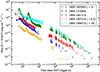 |
Fig. 1. Roughly the power-law shape (without a significant plateau) for the X-ray afterglow light curves of the GRBs with reported polarization detections. This fits well with the prediction of the hot fireball model. The slight deviation from the power law (breaks) can arise from the moderate viewing angle θv ∼ 1.5/Γ for the polarization sample (see Rossi et al. 2002). The early flares in GRB 140206A are inherited from prompt emission, considering a very close match for the light curves of Swift/BAT and Swift/XRT, during this period. |
2.2. T90 ∝ (Liso)−0.5 correlation for the prompt emission
In Figure 2, we show the T90 (intrinsic) and Liso (adopted from Xue et al. 2019) distribution for the GRBs with reported polarization detections, along with the high-efficiency sample and the high-energy sample. The sample with polarization and redshift detections (selected from Table 1 in Gill et al. 2021) consists of GRB 140206A, GRB 160131A, GRB 160509A, GRB 160623A, and GRB 171010A, and we only considered the main bright pulse when obtaining the T90 of GRB 120624B, GRB 160625B, and GRB 190114C in the high-energy sample. Obviously, the T90 ∝ (Liso)−0.5 correlation, found in Meng (2022), is available for all three samples (best fitted by log (T90) = 1.67–0.5 log (Liso) for a combined sample). In the following, we stress that this correlation is rather consistent with the prediction of the neutrino annihilation model – for neutrino-dominated accretion flow (NDAF; see Popham et al. 1999; Liu et al. 2017) –, and thus it favors the thermal-dominated jet and the photosphere model. The jet power of neutrino annihilation can be approximated as the following (for dimensionless black hole spin a = 0.95, see Zalamea & Beloborodov 2011; Leng & Giannios 2014):
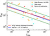 |
Fig. 2. T90 ∝ (Liso)−0.5 correlation (solid blue line) for the GRBs with reported polarization detections (red stars), along with the high-efficiency sample (orange stars; Meng 2022) and the high-energy sample (cyan stars; Eγ, beam ≳1052 erg, obtaining a GeV/TeV detection; Sharma et al. 2021). Notably, all three samples roughly exhibit a power-law shape in their X-ray afterglows. The dashed green lines mark a T90 deviation of a factor of two, from the best-fit log (T90) = 1.67–0.5 log (Liso) relationship. This T90 ∝ (Liso)−0.5 correlation aligns closely with the predictions made by the NDAF model (solid red line), which is under the hot fireball framework. |
 (1)
(1)
where Ṁign = 0.021 M⊙ s−1 (α/0.1)5/3 is the “ignition” accretion rate, Ṁtrap = 1.8 M⊙ s−1(α/0.1)1/3 is the “trapped” accretion rate, and α is the viscosity parameter of the neutrino-cooled disk. Note that  also depends on the dimensionless black hole spin a, and an analytical correlation of
 ![Mathematical equation: $ P_{\nu \overline{\nu}} \propto {[r_{\text{ ms}} (a)/r_{g}]}^{-4.8} $](/articles/aa/full_html/2026/02/aa56311-25/aa56311-25-eq3.gif) was obtained in Zalamea & Beloborodov (2011), based on the numerical simulations. Here, the a-dependent rms means the radius of the innermost stable orbit, rg = 2GM/c2, and rms(a)/rg ranges from 3 (a = 0) to 0.97 (a = 0.95). Additionally, other correlations have been proposed, such as
was obtained in Zalamea & Beloborodov (2011), based on the numerical simulations. Here, the a-dependent rms means the radius of the innermost stable orbit, rg = 2GM/c2, and rms(a)/rg ranges from 3 (a = 0) to 0.97 (a = 0.95). Additionally, other correlations have been proposed, such as  (see Xue et al. 2013).
As stated in Leng & Giannios (2014), the average accretion rate Ṁ during a burst can be approximated as  , assuming that the mass of the black hole roughly doubles through the accretion process. Also, it is considered that
  , where Liso is the observed isotropic equivalent luminosity from the jet, ϵ is the radiative efficiency, and θjet is the jet opening angle. Thus, the model-predicted Liso in the Ṁign < Ṁ < Ṁtrap regime for the long GRBs is the following (see also Equation (9) in Leng & Giannios 2014):
 (2)
(2)
where the reference values of ϵ = 0.3, θjet = 0.1, and MBH = 3 M⊙ were adopted. In the Ṁ > Ṁtrap regime, the optical depth of the neutrinos increased dramatically, and then the neutrinos were trapped in the accretion disk and advected onto the black hole (Di Matteo et al. 2002). So, the  and Liso rose much slower or were approximately constant (no T90 dependence was obtained; see Equation (1)).
As previously mentioned, the neutrino annihilation model predicts a T90 ∝ (Liso)−0.44 correlation. Considering ϵ≡ 0.9 for the high-efficiency sample, this model-predicted correlation (the red line in Figure 2, multiplied by 1.5) is thoroughly consistent with the above observation. Interestingly, in Figure 2, for a few bursts with the smallest T90 (less than 4 s), T90 drops much faster, close to T90 ∝ (Liso)−1. This can be naturally explained by the Ṁ ≳ Ṁtrap regime. On the one hand, the average accretion rate Ṁ for these bursts should be larger than 3 M⊙/(4s) (close to Ṁtrap). On the other hand, both the numerical simulations in Zalamea & Beloborodov (2011) (see Figure 4 therein; our adopted Equation (1) is a good analytical approximation derived from a simplified model) and in Lei et al. (2017) show that the luminosity (and  ) in this regime should not remain completely constant. According to the solid lines and points in Figure 1 of Lei et al. (2017), it is likely to exhibit a gradual rise as ∼Liso ∝ (Ṁ)1.0 ∝ (MBH/T90)1.0. Therefore, T90 ∝ (Liso)−1 was obtained.
It is particularly noteworthy that the above analysis favors a rather high dimensionless black hole spin of a = 0.95. In the next section, we find that the typical jet opening angle θjet for these bursts with higher energy could be two or three times smaller than 0.1 (θjet ∼ 0.03–0.05). Then, the spin may be smaller. If we consider Liso ∝ (10)2.45a (Xue et al. 2013), the spin can be ∼0.54–0.7. Regardless, the black hole spin is rather high, and the explicit value needs further exploration.
3. The apparent positive correlation of the low-energy spectral index α and the polarization degree
3.1. Observational results
Correlation between α and the polarization degree.
In Figure 3 (see also Table 1), we show the distribution of the low-energy spectral index α, for the GRBs with a reported polarization degree (omitting the upper and lower limits). This sample consists of the five bursts ultimately reported by POLAR (with an incoming angle below 45°, see Zhang et al. 2019), and five bursts reported by AstroSAT (five upper limits have been excluded, and GRB 160131A has been excluded due to the lack of Fermi/GBM detection; see Chattopadhyay et al. 2019). The low-energy spectral index was taken from Table 1 in Kole et al. (2020) for POLAR, and Table 1 in Chattopadhyay et al. (2019) for AstroSAT. Obviously, the low-energy spectral index α for most of these bursts (except for GRB 170101A in POLAR and GRB 160821A in AstroSAT) is rather hard, and rather close to or larger than the “synchrotron line of death” (α = −2/3; Preece et al. 1998). This terminology means that α should not exceed the value of −2/3 corresponding to the slow cooling limit for the synchrotron shock model. When considering much faster cooling of particles, α should be much softer, extending to a limit of −3/2. Thus, the polarization for these bursts is more likely to be produced by the photosphere emission. Note that we do not conclude that the polarization for all GRBs comes from the photosphere emission. However, for the polarization sample so far and in the near future, which has higher energy, the photosphere may be the more favorable mechanism. Also, notice that GRB 170101A is only detected by POLAR and Swift/BAT, and the best-fit peak energy Ep is quite large (323 keV, close to or beyond the detection upper limit), meaning that the best-fit model is actually the PL (power law) model. Thus, the low-energy spectral index α ≡ −1.55 is doubtful, or the origin of this burst may be special (with a high intrinsic luminosity and extremely large viewing angle).
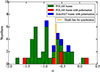 |
Fig. 3. Distribution of the low-energy spectral index α, for the GRBs with a reported polarization degree (the red and blue boxes, excluding the upper and lower limits). It is important to note that α is quite close to or larger than the “synchrotron line of death” α = −2/3 (the orange line). In addition, GRB 170101A is only detected by POLAR and Swift/BAT, and thus it is doubtful that α ≡ −1.55. |
In Figure 4a (see also Table 1), we illustrate the distribution of the low-energy spectral index α and the polarization degree, for the above four POLAR bursts (GRB 170101A is excluded) and five AstroSAT bursts. Interestingly, an obviously positive correlation of α and PD exists for both the POLAR sample and the AstroSAT sample. The Pearson correlation coefficient is r = 0.69 for the POLAR sample and r = 0.85 for the AstroSAT sample. Both are positive and larger than 0.6, indicating a strong positive correlation. In addition, the P values representing the significance level are both ∼0.06, thus the correlation is nearly significant (∼5%). When combining the data of POLAR and AstroSAT (accounting for their PD difference), P ∼ 0.03 (≤5%; then significant) can be achieved. It is worth mentioning that the higher polarization degree for AstroSAT may be due to its higher energy band and narrower bandwidth, considering the photosphere emission model (see Section 3.4). As stated in Section 1, Li & Shakeri (2025) obtained the nondependence of α and PD, ignoring the PD difference between POLAR and AstroSAT. Meanwhile, we considered a smaller and more reliable (likely) POLAR sample from Zhang et al. (2019), with additional criteria of higher fluence and a smaller incident angle of ≤45°. As explored in Section 3.3, we again achieved a positive correlation between α and PD, using a larger POLAR sample from Kole et al. (2020) alone.
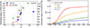 |
Fig. 4. Apparent positive correlation of the low-energy spectral index α and the polarization degree (left) and the possible photosphere explanation (right, polarization degree Π = |Q|/I). (a) Notably, this positive correlation can be obtained from both the POLAR sample (blue circles, with a Pearson correlation coefficient of r = 0.69) and the AstroSAT bursts (green triangles, r = 0.85). The P values standing for the significance level are both ∼0.06, and thus the correlation is almost significant (combining POLAR and AstroSAT, P ∼ 0.03 can be achieved). (b) For the photosphere polarization, the polarization degree is shown to be positively correlated with the p value (the power-law decreasing index of Γ, for the jet angular distribution), for the smaller θc, Γ case available for bursts with higher energy. Also, for Γ ⋅ θc, Γ ≃ 1, α is positively correlated with the p value, α ≃ ( − 1/4)(1 + 3/p). The predicted positive correlation of α and the polarization degree for θv = 0.015 (red pluses in the left panel) can match the observations of POLAR and the slope of the AstroSAT sample, approximately. Notice that GRB 170127C in POLAR may have larger θc, Γ, thus possessing a larger α of 0.25 and a smaller polarization degree (see Figure 5a, maybe two to three times smaller).
|
To further test the significance of the α-PD correlation, we performed a regression analysis and accounted for the uncertainties of the fitted parameters following Kelly et al. (2007). For the combined data of POLAR and AstroSAT (accounting for their PD difference by using a decreased factor for AstroSAT), we obtained PD = (10.79 ± 1.13)+(4.95 ± 1.87)⋅α, and thus the α dependence of PD is significant at 2.65σ. For the POLAR data alone, PD = (26.18 ± 1.88)+(32.47 ± 3.27)⋅α (omitting the outlier of GRB 170127C; 10σ) and PD = (10.37 ± 1.96)+(5.12 ± 3.82)⋅α (including GRB 170127C; 1.34σ) are achieved. For a larger POLAR sample (11 bursts) from Kole et al. (2020), 1.72σ was acquired (see Section 3.3). For the AstroSAT data alone, PD = (112.71 ± 15.28)+(63.70 ± 22.89)⋅α (significant at 2.78σ) was obtained. In addition, when adding more AstroSat bursts from Chattopadhyay et al. (2022) as stated in the next paragraph, the combined data of POLAR and AstroSAT could derive 3.05σ. According to the above results (≳2σ), we could claim that the positive correlation between α and PD is almost significant.
Notice that, for the five-year AstroSat polarization sample in Chattopadhyay et al. (2022), the correlation of α and the polarization degree has also been analyzed (see Figure 5b therein; for GRB 180103A, GRB 180120A, GRB 180427A, GRB 180914B, and GRB 190530A). They claim that no significant trend was observed. However, the apparent positive correlation exists without considering GRB 180103A (maybe GRB 180120A also). By carefully checking the properties of GRB 180103A, we think the inclusion is improper because of the following reasons: (1) the light curve of this burst appears as the complex multi-pulse (three or four pulses, with different shapes and amplitudes) structure, with an extremely long duration of T90 ∼ 165.83 s. The soft α = −1.31 is for the different pulses overlapping; for the single bright pulse (measured from T0 + 81.664 s to T0 + 93.952 s), α = −1.00 (see GCN Circular 22314). (2) This burst was only detected by Swift/BAT and Konus/Wind, and lacked any Fermi/GBM detection. Due to the relatively high low-energy cut of Konus/Wind (20 keV–20 MeV) and the low Ep ∼ 273 keV of this burst, the measured α = −1.00 is likely to suffer from the exponential component and thus mistakenly softer (α obtained from Konus/Wind seems to be softer than that from Fermi/GBM; see Figure 2b in Meng et al. 2024). (3) The incident angle of this burst is quite large, ∼52.33° (≳45°), so the polarization is greatly influenced by the interactions with the satellite elements. In addition, the light curve of GRB 180120A consists of two comparable peaks, and the error of the polarization degree is the largest among five bursts, 62.37 ± 29.79%.
The extremely hard α = −0.29 of GRB 180427A, significantly exceeding the “synchrotron line of death” and being obtained from Fermi/GBM, strongly supports its photosphere origin. Meanwhile, its polarization degree of 60.01 ± 22.32% is extraordinarily large. These two properties are well in line with GRB 160910A (α = −0.36) in the AstroSAT polarization sample, and GRB 170127C (α = 0.25) in the POLAR polarization sample (see Table 1). In addition, for the polarization sample of GAP (on board the IKAROS solar power sail; GRB 100826A, GRB 110301A, and GRB 110721A; Yonetoku et al. 2011, 2012), GRB 110721A is the well-known burst with a thermal component (Axelsson et al. 2012). Furthermore, α for GRB 100826A (α = −0.81 for Fermi/GBM, taken from Table 1 in Guan & Lan 2023; α = −0.84 for Konus-Wind; see GCN 11158) and GRB 110301A (α = −0.81 for Fermi/GBM; see GCN 11771) are both quite hard. Notice that several studies (e.g., Burgess et al. 2020) have shown that bursts with steep α can still be explained by synchrotron radiation.
3.2. Theoretical explanation
For synchrotron emission, with a locally ordered magnetic field (maximum linear polarization was obtained), the local polarization degree depends on the low-energy spectral (photon) index2α as (see Toma 2013; Gill et al. 2020 and Equation (10) in Gill et al. 2021)
 (3)
(3)
Thus, the softer α, the larger polarization is obtained. Namely, the negative correlation of α and the polarization degree is predicted, which contradicts the above observation. For other magnetic field structures (with a B⊥ component), the polarization degree is a fraction of the above maximum polarization, depending on the polar angle. So, this negative correlation should also be obtained.
For the nondissipative photospheric emission from a structured jet, the global polarization degree Π = |Q|/I can be calculated from the following (see also Equations (11) in Lundman et al. 2014):
 (4)
(4)
where Ω (θL, ϕL) are the angular coordinates of each local fluid element, relative to the LOS. In addition, ϕL = 0 indicates that the fluid element is in the plane of the LOS and the jet symmetric axis. Furthermore, D = [Γ(1 − β cos θL)]−1 is the Doppler factor, D2 stands for the angular probability distribution of emitting photons, and dṄ/dΩ is the angular distribution of the photon number (or luminosity) for the structured jet, with a jet boundary angle of θs (the solid angle is Ωs). Lastly, Π(θL) is the approximated polarization degree of each fluid element, taking the form of
 (5)
(5)
Here, the angular dependence comes from the Thompson scattering. A factor of 0.45 was adopted because the emission moving at a comoving angle of π/2 is shown to have Π ≈ 0.45 (rather than 1.0), which is close to and above the photosphere in a spherical outflow (see Figure 6 in Beloborodov 2011).
For this work, similar to previous works (Meng et al. 2019, 2022, 2024), we considered the structured jet with the following assumptions:
![Mathematical equation: $$ \begin{aligned} \left\{ \! \begin{array}{l} \Gamma (\theta ) =(\Gamma _{0}-1.2)/[(\theta /\theta _{c,\Gamma })^{2p}+1]^{1/2}+1.2, \\ L (\theta ) =L_{0}/[(\theta /\theta _{c,L})^{2q}+1]^{1/2}, \\ \theta _{c,\Gamma }<\theta _{c,L}, \ \ \theta _{v} < \theta _{c,L}. \end{array} \right. \end{aligned} $$](/articles/aa/full_html/2026/02/aa56311-25/aa56311-25-eq17.gif) (6)
(6)
Here, Γ(θ) represents the angular distribution for the Lorentz factor, Γ0 is the Lorentz factor in the center isotropic core, θc, Γ is the half opening angle of this Γ-constant core, and p denotes the power-law decreasing index of Γ outside the core. Similarly, L0 is the constant luminosity in the center core, and θc, L denotes the angular width for this core. In addition, θc, Γ < θc, L was accounted for based on the jet simulations (Zhang et al. 2003; Geng et al. 2019) and the enhanced material density at a larger angle (see detailed discussions in Meng et al. 2022). Normally, we expect θv < θc, L to observe the bright bursts (the observed luminosity has already dropped when θv > θc, Γ, since Γ decreases). For this case, the injected luminosity distribution can be approximated as angle-independent since the photospheric emission is emitted from a narrow region of ∼5/Γ (the jet boundary θs < =θc, L was adopted).
Based on Equation (4), in Figure 4b, with Γ0 = 100 and θc, Γ = 0.01 (θc, Γ * Γ0 = 1, narrower core), we show the photosphere polarization degree for different θv and p. A similar result for p = 4 can be seen in Figure 2 of Lundman et al. (2014). From Figure 4b, it is obvious that the polarization degree strongly depends on the p value. With a larger p value, a higher polarization degree is obtained.
It is particularly noteworthy that for the narrow core (θc, Γ * Γ0 < = 3), the low-energy spectral index α also strongly depends on the p value as (see also Equation (26) in Lundman et al. 2013)
 (7)
(7)
and it weakly depends on θv (see Figure 6 in Lundman et al. 2013 and Figure 3e in Meng et al. 2019). This equation indicates that, with a larger p value, the higher α is obtained. So, a positive correlation between α and the polarization degree is predicted theoretically.
To further test this, in Figure 4a, we plotted the theoretical distribution of α and the polarization degree for θv = 0.015 (see the other adopted parameters and the parameter dependence for PD in Figure 4b, Γ ⋅ θc, Γ = 1). It is clear that the observed correlation of POLAR and the slope of the AstroSAT sample can be explained. The GRB 170127C in POLAR may have larger θc, Γ, thus possessing a larger α of 0.25 and a smaller polarization degree (see Figure 5a, maybe two to three times smaller).
In Figure 5a, we compare the photosphere polarization degree for different θc, Γ, Γ ⋅ θc, Γ = 1 and Γ ⋅ θc, Γ = 2. A much larger polarization degree is predicted for smaller θc, Γ, with Γ ⋅ θc, Γ = 1. Also, in Figure 5b, we compare the observed θjet (taken from Du et al. 2021) for bursts with Eiso ≳ 1053 erg and Eiso ≲ 1053 erg, respectively. The θjet for the high-energy sample (Eiso ≳ 1053 erg) is shown to be significantly smaller, also implying θc, Γ. Note that this trend is thoroughly consistent with GRB 221009A – the brightest of all time (BOAT) burst–, which is claimed to possess an extremely narrow jet (∼1°, or 0.017 rad; see Cao 2023). Thus, for the high-energy bursts, the large flux should enhance the polarization detection and the smaller θc, Γ can increase the intrinsic polarization degree, which make them ideal candidates for polarization detection. Theoretically, the millisecond magnetar has a maximum rotational energy of ∼1052 erg to form a jet (Sharma et al. 2021). Thus, for the bursts with higher energy and a potential polarization detection, the central engine is more likely to be a black hole. Additionally, considering the probable power-law shape of the X-ray afterglow (see Figure 1), which matches the prediction of the hot fireball model, the photosphere origin of the prompt emission is preferred.
From Figure 4b and Figure 5a, it is evident that the jet has to be observed substantially off-axis (θv > θc, Γ) to obtain a significant polarization. This may imply an issue of explaining polarization with a photospheric model for which the off-axis observation ultimately causes an important reduction in the GRB luminosity. Especially when we try to explain the higher PD of AstroSAT (see Section 3.4), the θv ≳ 4 ⋅ θc, Γ condition may be considered. For the POLAR sample, we can effectively interpret it with θv ∼ 1.5 θc, Γ (see Figure 4a). In this case, for p = 3 (PD ∼12%), the observed Γ decreases by (1.5)p = 3.375 times and the luminosity (L ∝ Γ8/3) decreases by a factor of ∼25.6. Thus, the issue is not particularly significant in this condition.
3.3. α – PD distribution for a larger POLAR sample
To further check the α – PD correlation, in Figure 6, we show the α – PD distribution for a larger POLAR sample in Kole et al. (2020). We used 11 bursts with PD < 20°, omitting three obvious outliers (PD = 60 , 40
, 40 , and 21
 , respectively). Another motivation for the selection is that the photosphere polarization is typically < 20° (see Figure 4), unless the viewing angle is rather large (θv ≳ 3 ⋅ θc, Γ). From Figure 6, the positive correlation between α and PD is clearly obtained, which is best fitted by PD =(14.02 ± 1.81)+(4.24 ± 2.47)⋅α. Thus, it is nearly significant at 1.72σ. Notice that an approximate slope of 4.37 is achieved for the complete sample of 14 bursts. In addition, the best-fit slope remains positive for an arbitrary burst number, which is also available for the AstroSAT sample (combining the samples in Chattopadhyay et al. 2019 and Chattopadhyay et al. 2022).
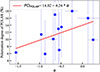 |
Fig. 6. The α – PD distribution for a larger POLAR sample (blue circles, 11 bursts) in Kole et al. (2020). It can be seen that the positive correlation between α and PD is quite obvious. The solid red line shows the best-fit correlation, which is PD = (14.02 ± 1.81)+(4.24 ± 2.47)⋅α. The correlation is almost significant, with a significance level of 1.72σ. |
3.4. Possible explanation for the higher PD of AstroSAT
In Figure 7a, considering the photosphere emission from a structured jet, we show the PD distribution for the emission from different local fluid elements (θLOS), relative to the LOS. Simplistically, the solid red line calculates the polarization degree for each fluid element of θLOS according to Equation (5), without considering the influence of azimuthal angle ϕLOS (namely ϕLOS = 0; Γ = 100 was adopted). More accurately, the blue boxes are the integrated results calculated from Equation (4), accounting for the influence of the azimuthal angle (ϕLOS was taken from 0 to 2 * π) and different specific θLOS intervals. Note that Γ = 100, θc, Γ = 0.01, θv = 0.015, and p = 4 were adopted. It can be seen that the polarization degree rapidly increases, peaks at around θLOS ∼ 1/Γ, and then falls quickly. So, the high polarization is almost within θLOS ∼ 1.5/Γ or ∼2/Γ. While the polarization degree from 1.5/Γ ≤ θLOS ≤ 5/Γ is much smaller. In Figure 7b, we compare the spectra emitted from 0 ≤ θLOS ≤ 1.5/Γ and 1.5/Γ ≤ θLOS ≤ 5/Γ. It was found that the spectrum from the inner region (0 ≤ θLOS ≤ 1.5/Γ; obtaining a higher PD) has higher energy. This may explain the higher PD of AstroSAT (100–600 keV), considering its higher band energy and narrower bandwidth than POLAR (50–500 keV).
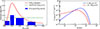 |
Fig. 7. Possible explanation for the PD discrepancy between POLAR and AstroSAT. (a) The PD distribution for the emission from different local fluid elements, relative to the light of sight. Note that Γ = 100, θc, Γ = 0.01, θv = 0.015, and p = 4 were adopted. The solid red line represents the polarization degree of each fluid element with θLOS, without considering the influence of the azimuthal angle ϕLOS (see Equation (5)). The blue boxes illustrate the integrated polarization degree for specific θLOS intervals, considering the influence of the azimuthal angle. The polarization degree obviously rises rapidly, peaks at around θLOS ∼ 1/Γ, and then drops down quickly. The high polarization is almost within ∼1.5/Γ or ∼2/Γ. The dashed green line marks the total polarization degree for 0 ≤ θLOS ≤ 0.1. (b) The comparison of the spectra emitted from 0 ≤ θLOS ≤ 1.5/Γ and 1.5/Γ ≤ θLOS ≤ 5/Γ (Γ = 200, Γ ⋅ θc, Γ = 1, and θv = 1.5/Γ were adopted). Obviously, the spectrum from the inner region (0 ≤ θLOS ≤ 1.5/Γ) has higher energy and a higher PD (as can be seen in the left panel). This may contribute to the larger PD of AstroSAT (100–600 keV), due to its higher band energy and narrower bandwidth than POLAR (50–500 keV). The narrow bandwidth of ∼6 times ultimately enables only the detection of the high-energy component from the inner region (the right portion of the blue line). |
Except for the above origin, there can be two other effects contributing to the higher PD of AstroSAT. First, as stated in Chattopadhyay et al. (2022), the narrower bandwidth and higher band energy of AstroSAT may result in a shorter burst duration, which prevents the PD decrease originating from spectral overlapping across the burst duration. In Parsotan & Lazzati (2022), the PD of the time-resolved spectrum was indeed found to be larger than that of the time-integrated spectrum, based on the Monte Carlo simulations for photosphere emission. Second, the distribution for AstroSAT (with higher PD) could also be explained with a larger θv (θv ≳ 0.04, see Figure 4b), considering the similar slope of α−PD distributions for POLAR and AstroSAT. It is possible that AstroSAT has a lower sensitivity for polarization detections. If so, the high-polarization bursts with larger θv would be achieved, leaving the low-polarization bursts unconstrained. In addition to the comparison between POLAR and AstroSAT, we should deal with the high PD values of AstroSAT (all higher than 45%). As shown in Equation (5), we adopted the factor of 0.45, corresponding to the PD at a comoving angle of π/2 and τ = 1 in a spherical outflow. However, the emission from τ ≳ 1 also contributes to the probability photosphere model, which could have Π≈ 0.6 (see Figure 6 in Beloborodov 2011). Also, when the structured jet is considered, Π could be much larger due to an increased asymmetry. Notice that the photosphere polarization in the γ-ray band is claimed to reach 75% or even higher in some intervals, as shown in Figure 2 in Parsotan & Lazzati (2022).
4. Summary and discussion
The radiation mechanism (thermal photosphere or magnetic synchrotron) of GRB prompt emission is tricky to distinguish. Considering the particular jet structure (with an angular distribution, especially for the Lorentz factor; Pe’er 2008; Pe’er & Ryde 2011; Meng et al. 2024) for the photosphere model or the specified magnetic field structure (with radial decay; Zhang & Yan 2011; Geng et al. 2018; Yan et al. 2024), the observed GRB spectrum can be reproduced. Meanwhile, the polarization observation is crucial to diagnose the jet structure or the magnetic field configuration. So far, the polarization measurements for the prompt emission of GRBs have been reported by the IKAROS-GAP (50–300 keV; Yonetoku et al. 2011, 2012), the AstroSat-CZTI (100–600 keV; Chattopadhyay et al. 2019, 2022), and the POLAR missions (50–500 keV; Zhang et al. 2019).
In this work, based on the observational results of POLAR and AstroSAT, we explore the characteristics of the X-ray afterglow shape, the prompt emission (T90 vs. Liso, α), and the polarization degree (polarization degree vs. α), for the GRBs with a reported polarization detection. The following results are revealed. First, the X-ray afterglows show a power-law shape and T90 ∝ (Liso)−0.5 correlation exists, consistent with the predictions of the classical fireball model and the neutrino annihilation model (NDAF), respectively. Second, the low-energy spectral index α was found to be rather hard, including the GAP sample and especially GRB 160910A (α = −0.36), GRB 170127C (α = 0.25), and GRB 180427A (α = −0.29). Third, we find the positive correlation of the α and the polarization degree. The bursts with the hardest α (such as GRB 160910A and GRB 170127C) possess the highest polarization degree. Fourth, for the structured jet and large viewing angle, the symmetry break of photon scattering overlapping should invoke a certain photosphere polarization. Based on this consideration, adopting Γ ⋅ θc, Γ = 1 and different p values for the jet structure and viewing angle of θv = 0.015, we interpret the above positive correlation. With a larger p value, α is much harder (≃ − (1 + 3/p)/4), and the polarization degree is much higher due to enhanced asymmetry.
The positive correlation of α and the polarization degree can be further tested by the future GRB polarization missions, such as LEAP (50–500 keV, NASA Mission; McConnell et al. 2021) and POLAR-2 (de Angelis & Polar-2 Collaboration 2022). POLAR-2 is planned to be deployed on the China Space Station (CSS) in 2026, and consists of three detectors: a Low-energy X-ray Polarization Detector (LPD, 2–10 keV; Feng et al. 2023, 2024; Yi et al. 2024) and a Broad-spectrum Detector (BSD, 8–2000 keV) developed in China, as well as a High-energy X-ray Polarization Detector (HPD, 30–800 keV; Hulsman 2020) developed in Europe. However, caution should be taken. First, from our theoretical point, the correlation is valid for relatively small θc, Γ and a moderate viewing angle (θv ≲ 3θc, Γ), which can be available for most GRBs (Lundman et al. 2013; Meng et al. 2019) and especially for the bright bursts capable of polarization detection. However, with a larger polarization sample, some outliers with large θv (much softer α = −1.5 and a higher polarization degree can be obtained, maybe for GRB 170101A) or large θc, Γ (with hard α and a smaller polarization degree; see Figure 5a) may exist. We can judge the structure condition better by combining the spectral evolutions (Meng et al. 2019). Second, just as GRB 180103A, some bursts with an extremely complex light curve (multiple episodes) can be included. If so, the used α should not correspond to the time-integrated spectrum.
The origin of the GRB polarization is still puzzling, which may be produced by synchrotron emission with an ordered magnetic field, photosphere emission, or the Compton drag effect. For GRB 160910A, GRB 170127C and GRB 180427A (with α ≳ −0.36), and GRB 110721A (with a blackbody component), we consider their polarization to be likely caused by photosphere emission with jet asymmetry. In addition to the correlation of α and the polarization degree for the time-integrated spectrum, we will expand the studies of the photosphere polarization in future works. On the one hand, the time evolution of the polarization properties and comparison with the spectral evolution should be further explored, along with the rotation of the PA in GRB 170114A and GRB 160821A (Li et al. 2024; Wang et al. 2024). On the other hand, the energy dependence of the polarization degree (namely the polarization spectrum) should be investigated in great detail. If so, it could be further checked by the wide-band observation of POLAR-2.
Acknowledgments
We thank Bin-Bin Zhang for the useful discussions. We acknowledge the use of the GRB data from Fermi/GBM, POLAR, and AstroSAT. Y. Z. M. is supported by the National Natural Science Foundation of China (grant No. 12403045), the Natural Science Foundation of Guangxi (grant No. 2025GXNSFBA069091), and the Starting Foundation of Guangxi University of Science and Technology (grant No. 24Z01). S. Q. Z. is supported by the National Natural Science Foundation of China (grant No. 12503048) and the Starting Foundation of Guangxi University of Science and Technology (grant No. 24Z17). X. F. L. is supported by the National Natural Science Foundation of China (grant No. 12565008).
References
- Abdo, A. A., Ackermann, M., Ajello, M., et al. 2009, ApJ, 706, L138 [NASA ADS] [CrossRef] [Google Scholar]
- Acuner, Z., Ryde, F., Pe’er, A., et al. 2020, ApJ, 893, 128 [NASA ADS] [CrossRef] [Google Scholar]
- Ahlgren, B., Larsson, J., Nymark, T., et al. 2015, MNRAS, 454, L31 [Google Scholar]
- Amati, L., Frontera, F., Tavani, M., et al. 2002, A&A, 390, 81 [NASA ADS] [CrossRef] [EDP Sciences] [Google Scholar]
- Axelsson, M., & Borgonovo, L. 2015, MNRAS, 447, 3150 [NASA ADS] [CrossRef] [Google Scholar]
- Axelsson, M., Baldini, L., Barbiellini, G., et al. 2012, ApJ, 757, L31 [CrossRef] [Google Scholar]
- Band, D., Matteson, J., Ford, L., et al. 1993, ApJ, 413, 281 [Google Scholar]
- Beloborodov, A. M. 2011, ApJ, 737, 68 [NASA ADS] [CrossRef] [Google Scholar]
- Burgess, J. M. 2019, A&A, 629, A69 [NASA ADS] [CrossRef] [EDP Sciences] [Google Scholar]
- Burgess, J. M., Kole, M., Berlato, F., et al. 2019, A&A, 627, A105 [NASA ADS] [CrossRef] [EDP Sciences] [Google Scholar]
- Burgess, J. M., Bégué, D., Greiner, J., et al. 2020, Nat. Astron., 4, 174 [Google Scholar]
- Chattopadhyay, T., Vadawale, S. V., Aarthy, E., et al. 2019, ApJ, 884, 123 [NASA ADS] [CrossRef] [Google Scholar]
- Chattopadhyay, T., Gupta, S., Iyyani, S., et al. 2022, ApJ, 936, 12 [NASA ADS] [CrossRef] [Google Scholar]
- Coburn, W., & Boggs, S. E. 2003, Nature, 423, 415 [Google Scholar]
- Covino, S., & Gotz, D. 2016, Astron. Astrophys. Trans., 29, 205 [NASA ADS] [Google Scholar]
- de Angelis, N., & Polar-2 Collaboration 2022, 37th International Cosmic Ray Conference, 580 [Google Scholar]
- Deng, W., Zhang, H., Zhang, B., & Li, H. 2016, ApJ, 821, L12 [NASA ADS] [CrossRef] [Google Scholar]
- Dereli-Bégué, H., Pe’er, A., & Ryde, F. 2020, ApJ, 897, 145 [Google Scholar]
- Di Matteo, T., Perna, R., & Narayan, R. 2002, ApJ, 579, 706 [Google Scholar]
- Du, M., Yi, S.-X., Liu, T., Song, C.-Y., & Xie, W. 2021, ApJ, 908, 242 [NASA ADS] [CrossRef] [Google Scholar]
- Feng, H., Liu, H., Liu, S., et al. 2023, Nucl. Instrum. Methods Phys. Res. A, 1055, 168499 [Google Scholar]
- Feng, Z.-K., Liu, H.-B., Xie, F., et al. 2024, ApJ, 960, 87 [Google Scholar]
- Geng, J.-J., Huang, Y.-F., Wu, X.-F., Zhang, B., & Zong, H.-S. 2018, ApJS, 234, 3 [Google Scholar]
- Geng, J.-J., Zhang, B., Kölligan, A., Kuiper, R., & Huang, Y.-F. 2019, ApJ, 877, L40 [CrossRef] [Google Scholar]
- Gill, R., Granot, J., & Kumar, P. 2020, MNRAS, 491, 3343 [Google Scholar]
- Gill, R., Kole, M., & Granot, J. 2021, Galaxies, 9, 82 [NASA ADS] [CrossRef] [Google Scholar]
- Goodman, J. 1986, ApJ, 308, L47 [NASA ADS] [CrossRef] [Google Scholar]
- Gowri, A., Pe’er, A., Ryde, F., et al. 2025, ApJ, 991, 230 [Google Scholar]
- Granot, J. 2003, ApJ, 596, L17 [NASA ADS] [CrossRef] [Google Scholar]
- Guan, R. Y., & Lan, M. X. 2023, A&A, 670, A160 [NASA ADS] [CrossRef] [EDP Sciences] [Google Scholar]
- Hulsman, J. 2020, SPIE Conf. Ser., 11444, 114442V [Google Scholar]
- Ito, H., Matsumoto, J., Nagataki, S., et al. 2024, ApJ, 961, 243 [Google Scholar]
- Kaneko, Y., Preece, R. D., Briggs, M. S., et al. 2006, ApJS, 166, 298 [CrossRef] [Google Scholar]
- Kelly, B. C., Bechtold, J., Siemiginowska, A., et al. 2007, ApJ, 657, 116 [Google Scholar]
- Kole, M., De Angelis, N., Berlato, F., et al. 2020, A&A, 644, A124 [NASA ADS] [CrossRef] [EDP Sciences] [Google Scholar]
- Lan, M.-X., Geng, J.-J., Wu, X.-F., & Dai, Z.-G. 2019, ApJ, 870, 96 [NASA ADS] [CrossRef] [Google Scholar]
- Lan, M.-X., Wang, H.-B., Xu, S., Liu, S., & Wu, X.-F. 2021, ApJ, 909, 184 [NASA ADS] [CrossRef] [Google Scholar]
- Lei, W.-H., Zhang, B., Wu, X.-F., & Liang, E.-W. 2017, ApJ, 849, 47 [NASA ADS] [CrossRef] [Google Scholar]
- Leng, M., & Giannios, D. 2014, MNRAS, 445, L1 [Google Scholar]
- LHAASO Collaboration (Cao, Z. et al.) 2023, Science, 380, 1390 [NASA ADS] [CrossRef] [Google Scholar]
- Li, L., & Shakeri, S. 2025, ApJS, 276, 9 [Google Scholar]
- Li, J.-S., Wang, H.-B., & Lan, M.-X. 2024, ApJ, 973, 2 [NASA ADS] [CrossRef] [Google Scholar]
- Liu, T., Gu, W.-M., & Zhang, B. 2017, New Astron. Rev., 79, 1 [Google Scholar]
- Lundman, C., Pe’er, A., & Ryde, F. 2013, MNRAS, 428, 2430 [NASA ADS] [CrossRef] [Google Scholar]
- Lundman, C., Pe’er, A., & Ryde, F. 2014, MNRAS, 440, 3292 [NASA ADS] [CrossRef] [Google Scholar]
- Lyutikov, M., Pariev, V. I., & Blandford, R. D. 2003, ApJ, 597, 998 [Google Scholar]
- McConnell, M. L., Baring, M., Bloser, P., et al. 2021, SPIE Conf. Ser., 11821, 118210P [Google Scholar]
- Meng, Y.-Z. 2022, ApJS, 263, 39 [Google Scholar]
- Meng, Y.-Z., Geng, J.-J., Zhang, B.-B., et al. 2018, ApJ, 860, 72 [NASA ADS] [CrossRef] [Google Scholar]
- Meng, Y.-Z., Liu, L.-D., Wei, J.-J., Wu, X.-F., & Zhang, B.-B. 2019, ApJ, 882, 26 [NASA ADS] [CrossRef] [Google Scholar]
- Meng, Y.-Z., Geng, J.-J., & Wu, X.-F. 2022, MNRAS, 509, 6047 [Google Scholar]
- Meng, Y.-Z., Wang, X. I., & Liu, Z.-K. 2024, ApJ, 963, 112 [Google Scholar]
- Mészáros, P. 2002, ARA&A, 40, 137 [CrossRef] [Google Scholar]
- Mészáros, P., & Rees, M. J. 1997, ApJ, 476, 232 [CrossRef] [Google Scholar]
- Paczynski, B. 1986, ApJ, 308, L43 [NASA ADS] [CrossRef] [Google Scholar]
- Paczynski, B., & Rhoads, J. E. 1993, ApJ, 418, L5 [NASA ADS] [CrossRef] [Google Scholar]
- Parsotan, T., & Lazzati, D. 2022, ApJ, 926, 104 [NASA ADS] [CrossRef] [Google Scholar]
- Parsotan, T., López-Cámara, D., & Lazzati, D. 2020, ApJ, 896, 139 [NASA ADS] [CrossRef] [Google Scholar]
- Pe’er, A. 2008, ApJ, 682, 463 [NASA ADS] [CrossRef] [Google Scholar]
- Pe’er, A., & Ryde, F. 2011, ApJ, 732, 49 [CrossRef] [Google Scholar]
- Pe’er, A., Zhang, B.-B., Ryde, F., et al. 2012, MNRAS, 420, 468 [Google Scholar]
- Piran, T. 1999, Phys. Rep., 314, 575 [NASA ADS] [CrossRef] [Google Scholar]
- Popham, R., Woosley, S. E., & Fryer, C. 1999, ApJ, 518, 356 [NASA ADS] [CrossRef] [Google Scholar]
- Preece, R. D., Briggs, M. S., Mallozzi, R. S., et al. 1998, ApJ, 506, L23 [Google Scholar]
- Rees, M. J., & Mészáros, P. 2005, ApJ, 628, 847 [NASA ADS] [CrossRef] [Google Scholar]
- Rossi, E., Lazzati, D., & Rees, M. J. 2002, MNRAS, 332, 945 [NASA ADS] [CrossRef] [Google Scholar]
- Ruffini, R., Siutsou, I. A., & Vereshchagin, G. V. 2013, ApJ, 772, 11 [Google Scholar]
- Ryde, F., & Pe’er, A. 2009, ApJ, 702, 1211 [NASA ADS] [CrossRef] [Google Scholar]
- Ryde, F., Axelsson, M., Zhang, B. B., et al. 2010, ApJ, 709, L172 [Google Scholar]
- Ryde, F., Lundman, C., & Acuner, Z. 2017, MNRAS, 472, 1897 [Google Scholar]
- Samuelsson, F., & Ryde, F. 2023, ApJ, 956, 42 [NASA ADS] [CrossRef] [Google Scholar]
- Sharma, V., Iyyani, S., & Bhattacharya, D. 2021, ApJ, 908, L2 [Google Scholar]
- Toma, K. 2013, ArXiv e-prints [arXiv:1308.5733] [Google Scholar]
- Toma, K., Sakamoto, T., Zhang, B., et al. 2009, ApJ, 698, 1042 [NASA ADS] [CrossRef] [Google Scholar]
- Tuo, J.-C., Liu, H.-B., Mai, Q.-N., et al. 2024, ApJ, 973, 113 [Google Scholar]
- Wang, X., Lan, M.-X., Tang, Q.-W., Wu, X.-F., & Dai, Z.-G. 2024, ApJ, 972, 15 [NASA ADS] [CrossRef] [Google Scholar]
- Waxman, E. 2003, Nature, 423, 388 [NASA ADS] [CrossRef] [Google Scholar]
- Xue, L., Liu, T., Gu, W.-M., & Lu, J.-F. 2013, ApJS, 207, 23 [Google Scholar]
- Xue, L., Zhang, F.-W., & Zhu, S.-Y. 2019, ApJ, 876, 77 [NASA ADS] [CrossRef] [Google Scholar]
- Yamazaki, R., Sato, Y., Sakamoto, T., & Serino, M. 2020, MNRAS, 494, 5259 [Google Scholar]
- Yan, Z.-Y., Yang, J., Zhao, X.-H., Meng, Y.-Z., & Zhang, B.-B. 2024, ApJ, 962, 85 [NASA ADS] [CrossRef] [Google Scholar]
- Yi, D., Liu, Q., Liu, H., et al. 2024, ArXiv e-prints [arXiv:2407.14243] [Google Scholar]
- Yonetoku, D., Murakami, T., Gunji, S., et al. 2011, ApJ, 743, L30 [NASA ADS] [CrossRef] [Google Scholar]
- Yonetoku, D., Murakami, T., Gunji, S., et al. 2012, ApJ, 758, L1 [NASA ADS] [CrossRef] [Google Scholar]
- Zalamea, I., & Beloborodov, A. M. 2011, MNRAS, 410, 2302 [Google Scholar]
- Zhang, B. 2020, Nat. Astron., 4, 210 [NASA ADS] [CrossRef] [Google Scholar]
- Zhang, B., & Yan, H. 2011, ApJ, 726, 90 [Google Scholar]
- Zhang, W., Woosley, S. E., & MacFadyen, A. I. 2003, ApJ, 586, 356 [CrossRef] [Google Scholar]
- Zhang, B.-B., Zhang, B., Liang, E.-W., et al. 2011, ApJ, 730, 141 [NASA ADS] [CrossRef] [Google Scholar]
- Zhang, S.-N., Kole, M., Bao, T.-W., et al. 2019, Nat. Astron., 3, 258 [CrossRef] [Google Scholar]
Notice that, as stated in Burgess (2019), some narrow spectra can also be fitted by the physical synchrotron model. The width measure can suffer from the poor fit of the empirical Band function, and the smoothly broken power law (SBPL) model with a variable curvature parameter Δ could be a better model.
Note that in several works involving the polarization of synchrotron emission (Gill et al. 2020; Guan & Lan 2023), the low-energy spectral index αs stands for the flux spectrum, and α = −αs − 1.
All Tables
All Figures
|
Fig. 1. Roughly the power-law shape (without a significant plateau) for the X-ray afterglow light curves of the GRBs with reported polarization detections. This fits well with the prediction of the hot fireball model. The slight deviation from the power law (breaks) can arise from the moderate viewing angle θv ∼ 1.5/Γ for the polarization sample (see Rossi et al. 2002). The early flares in GRB 140206A are inherited from prompt emission, considering a very close match for the light curves of Swift/BAT and Swift/XRT, during this period. |
| In the text | |
|
Fig. 2. T90 ∝ (Liso)−0.5 correlation (solid blue line) for the GRBs with reported polarization detections (red stars), along with the high-efficiency sample (orange stars; Meng 2022) and the high-energy sample (cyan stars; Eγ, beam ≳1052 erg, obtaining a GeV/TeV detection; Sharma et al. 2021). Notably, all three samples roughly exhibit a power-law shape in their X-ray afterglows. The dashed green lines mark a T90 deviation of a factor of two, from the best-fit log (T90) = 1.67–0.5 log (Liso) relationship. This T90 ∝ (Liso)−0.5 correlation aligns closely with the predictions made by the NDAF model (solid red line), which is under the hot fireball framework. |
| In the text | |
|
Fig. 3. Distribution of the low-energy spectral index α, for the GRBs with a reported polarization degree (the red and blue boxes, excluding the upper and lower limits). It is important to note that α is quite close to or larger than the “synchrotron line of death” α = −2/3 (the orange line). In addition, GRB 170101A is only detected by POLAR and Swift/BAT, and thus it is doubtful that α ≡ −1.55. |
| In the text | |
|
Fig. 4. Apparent positive correlation of the low-energy spectral index α and the polarization degree (left) and the possible photosphere explanation (right, polarization degree Π = |Q|/I). (a) Notably, this positive correlation can be obtained from both the POLAR sample (blue circles, with a Pearson correlation coefficient of r = 0.69) and the AstroSAT bursts (green triangles, r = 0.85). The P values standing for the significance level are both ∼0.06, and thus the correlation is almost significant (combining POLAR and AstroSAT, P ∼ 0.03 can be achieved). (b) For the photosphere polarization, the polarization degree is shown to be positively correlated with the p value (the power-law decreasing index of Γ, for the jet angular distribution), for the smaller θc, Γ case available for bursts with higher energy. Also, for Γ ⋅ θc, Γ ≃ 1, α is positively correlated with the p value, α ≃ ( − 1/4)(1 + 3/p). The predicted positive correlation of α and the polarization degree for θv = 0.015 (red pluses in the left panel) can match the observations of POLAR and the slope of the AstroSAT sample, approximately. Notice that GRB 170127C in POLAR may have larger θc, Γ, thus possessing a larger α of 0.25 and a smaller polarization degree (see Figure 5a, maybe two to three times smaller).
|
||
| In the text | |||
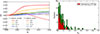 |
Fig. 5. Correlations of photosphere polarization degree (Π = |Q|/I), θc, Γ (or θjet), and Eiso. (a) Comparison of the photosphere polarization degree for smaller θc, Γ (Γ ⋅ θc, Γ = 1, solid lines; predicting a much larger polarization degree) and larger θc, Γ (Γ ⋅ θc, Γ = 2, dashed lines; predicting a much smaller polarization degree). (b) The smaller θjet (likely θc, Γ also) is found for the high-energy sample (Eiso ≳ 1053 erg), indicating the polarization detection. |
| In the text | |
|
Fig. 6. The α – PD distribution for a larger POLAR sample (blue circles, 11 bursts) in Kole et al. (2020). It can be seen that the positive correlation between α and PD is quite obvious. The solid red line shows the best-fit correlation, which is PD = (14.02 ± 1.81)+(4.24 ± 2.47)⋅α. The correlation is almost significant, with a significance level of 1.72σ. |
| In the text | |
|
Fig. 7. Possible explanation for the PD discrepancy between POLAR and AstroSAT. (a) The PD distribution for the emission from different local fluid elements, relative to the light of sight. Note that Γ = 100, θc, Γ = 0.01, θv = 0.015, and p = 4 were adopted. The solid red line represents the polarization degree of each fluid element with θLOS, without considering the influence of the azimuthal angle ϕLOS (see Equation (5)). The blue boxes illustrate the integrated polarization degree for specific θLOS intervals, considering the influence of the azimuthal angle. The polarization degree obviously rises rapidly, peaks at around θLOS ∼ 1/Γ, and then drops down quickly. The high polarization is almost within ∼1.5/Γ or ∼2/Γ. The dashed green line marks the total polarization degree for 0 ≤ θLOS ≤ 0.1. (b) The comparison of the spectra emitted from 0 ≤ θLOS ≤ 1.5/Γ and 1.5/Γ ≤ θLOS ≤ 5/Γ (Γ = 200, Γ ⋅ θc, Γ = 1, and θv = 1.5/Γ were adopted). Obviously, the spectrum from the inner region (0 ≤ θLOS ≤ 1.5/Γ) has higher energy and a higher PD (as can be seen in the left panel). This may contribute to the larger PD of AstroSAT (100–600 keV), due to its higher band energy and narrower bandwidth than POLAR (50–500 keV). The narrow bandwidth of ∼6 times ultimately enables only the detection of the high-energy component from the inner region (the right portion of the blue line). |
| In the text | |
Current usage metrics show cumulative count of Article Views (full-text article views including HTML views, PDF and ePub downloads, according to the available data) and Abstracts Views on Vision4Press platform.
Data correspond to usage on the plateform after 2015. The current usage metrics is available 48-96 hours after online publication and is updated daily on week days.
Initial download of the metrics may take a while.