| Issue |
A&A
Volume 706, February 2026
|
|
|---|---|---|
| Article Number | A203 | |
| Number of page(s) | 16 | |
| Section | Stellar structure and evolution | |
| DOI | https://doi.org/10.1051/0004-6361/202556315 | |
| Published online | 10 February 2026 | |
Observational probes of the neutron star equation of state with hyperons, bosonic dark matter, and quark matter
1
Institute for Theoretical Physics, University of Wrocław Plac Maksa Borna 9 50-204 Wrocław, Poland
2
Incubator of Scientific Excellence, Center for Simulations of Superdense Fluids, University of Wrocław Plac Maksa Borna 9 50-204 Wrocław, Poland
3
Frankfurt Institute for Advanced Studies, Giersch Science Center D-60438 Frankfurt am Main, Germany
4
Alikhanyan National Science Laboratory (Yerevan Institute of Physics) Alikhanyan Brothers St 2 0036 Yerevan, Armenia
5
Technische Universität Darmstadt, Fachbereich Physik, Institut für Kernphysik Schlossgartenstraße 9 D-64289 Darmstadt, Germany
6
GSI Helmholtzzentrum für Schwerionenforschung GmbH, Theorie Planckstraße 1 D-64291 Darmstadt, Germany
★ Corresponding authors: This email address is being protected from spambots. You need JavaScript enabled to view it.
, This email address is being protected from spambots. You need JavaScript enabled to view it.
, This email address is being protected from spambots. You need JavaScript enabled to view it.
Received:
8
July
2025
Accepted:
30
October
2025
Abstract
Context. The presence of dark matter in neutron stars is of growing interest due to its potential impact on the structure and observable properties of these objects. Among the various candidates, the hypothetical sexaquark has emerged as a promising bosonic dark matter particle, potentially forming under extreme conditions in neutron star cores.
Aims. We investigate whether a hybrid neutron star model that includes hyperons, bosonic dark matter (in the form of sexaquarks), and deconfined quark matter can satisfy all current observational constraints. We particularly focus on identifying the range of sexaquark masses consistent with mass-radius measurements and the tidal deformability limit.
Methods. We used the DD2Y-T model for the hadronic phase, which includes hyperons, and a nonlocal Nambu–Jona-Lasinio model for the deconfined quark phase. The phase transition was modeled as a smooth crossover using the replacement interpolation construction method. Sexaquark-baryon interactions were introduced via an effective mass shift representing repulsion. We incorporated the full set of current observational data, including NICER measurements of PSRs J0437–4715 and newly published J0614–3329 data, and performed a Bayesian analysis to constrain the sexaquark mass.
Results. Our results show that the presence of the sexaquark softens the equation of state, enabling the hybrid model to satisfy both the radius and tidal deformability constraints around the canonical 1.4 M⊙ neutron stars. We find that hybrid EOSs with a sexaquark mass around 1900 MeV are in agreement with all available constraints, including those from HESS J1731–347 and PSR J0952–0607, which represent the lowest and highest mass neutron stars observed to date. The Bayesian analysis favors a sexaquark mass range of 1885–1935 MeV, supporting the potential relevance of this exotic particle in neutron star interiors.
Key words: dense matter / equation of state / stars: neutron
© The Authors 2026
 Open Access article, published by EDP Sciences, under the terms of the Creative Commons Attribution License (https://creativecommons.org/licenses/by/4.0), which permits unrestricted use, distribution, and reproduction in any medium, provided the original work is properly cited.
This article is published in open access under the Subscribe to Open model. This email address is being protected from spambots. You need JavaScript enabled to view it. to support open access publication.
1. Introduction
The accepted cosmological models that are presented and founded in general gelativity (GR) suggest that almost 27% of the matter-energy composition of the Universe exists in the form of enigmatic dark matter (DM; Bertone & Hooper 2018; de Martino et al. 2020). Multi-messenger astrophysics is actively engaged in the search for and examination of new ideas concerning DM particles. These candidates are believed to be non-relativistic particles that exist beyond the Standard Model of particle physics. They interact weakly with ordinary baryonic matter (BM) solely through gravitational forces (Salucci et al. 2021; Arbey & Mahmoudi 2021). In this context, weakly interacting massive particles are one of the notable DM candidates (Bertone & Tait 2018; Arcadi et al. 2018). Moreover, hypothetical bosonic particles such as the axion (Marsh 2016; Chadha-Day et al. 2022) and the sexaquark (S; Farrar 2022; Doser et al. 2023; Moore & Slatyer 2024) also exhibit the primary characteristics required to be considered potential DM candidates. Their interaction with the BM must be very weak, which is why they have remained undetected thus far. The mass of candidate DM particles spans a wide range, from approximately 10−22 eV to 1010 eV, and is based on the particular type of candidate (Cirelli et al. 2024). Moreover, their self-interaction is another key parameter of the DM model. Indeed, self-interacting DM has the potential to address several issues in cosmology and astrophysics, including “core-cusp”, “missing satellite”, and “too big to fail” problems (Spergel & Steinhardt 2000; Peter et al. 2013; Kaplinghat et al. 2016). Given these model parameters, DM particles must be incorporated into an equation of state (EOS), which is a fundamental tool for characterizing matter.
It is believed that gravitationally stable astrophysical objects composed of DM could form in the Universe (Liebling & Palenzuela 2023; Baryakhtar et al. 2022; Visinelli 2021). In this context, they can exist as an object made entirely of DM, so-called dark stars (Narain et al. 2006; Maselli et al. 2017). Such objects include axion stars, boson stars (Eby et al. 2016; Visinelli et al. 2018; Pitz & Schaffner-Bielich 2023), and stars that have a fraction of DM mixed with BM (Bramante & Raj 2024). For the last type, compact objects such as black holes (Shakeri & Hajkarim 2023), neutron stars (NSs; (Karkevandi et al. 2022; Shakeri & Karkevandi 2024)), white dwarfs (Ryan & Radice 2022), and even hypothetical quark (strange) stars (Ferreira & Fraga 2023; Yang & Pi 2024; Sedaghat et al. 2025; Liu et al. 2025a) offer a significant opportunity to probe DM indirectly. These objects are considered promising astrophysical environments where DM may reside, either within them or in a surrounding halo.
Neutron stars, due to their extreme gravitational potential and high baryon density, have the potential to accumulate DM particles and are widely regarded as astrophysical laboratories for studying DM (Grippa et al. 2025). In recent years, motivated by new and significant observational data on NS properties, numerous studies have investigated the possible presence of DM within these objects (Ivanytskyi et al. 2020; Rafiei Karkevandi et al. 2021; Dengler et al. 2022; Rutherford et al. 2023; Karkevandi et al. 2024; Thakur et al. 2024; Konstantinou 2024; Routaray et al. 2025; Biesdorf et al. 2025; Arvikar et al. 2025). The influence of DM on observable features of NSs has been explored in order to place constraints on the parameter space of DM models (Sedrakian 2016, 2019; Shakeri & Karkevandi 2024; Giangrandi et al. 2023; Diedrichs et al. 2023; Ávila et al. 2024; Issifu et al. 2025; Cipriani et al. 2025; Scordino & Bombaci 2025; Mukherjee et al. 2025). Furthermore, unusual measurements of NS mass and radius have prompted attempts to explain them in terms of mixed configurations, hereafter referred to as DM admixed NSs. In this direction, HESS J1731–347 (Sagun et al. 2023; Marzola et al. 2025) and XTE J1814-338 ultracompact stars (Pitz & Schaffner-Bielich 2025; Yang et al. 2025; Lopes & Issifu 2025) as well as very massive compact objects, such as the secondary ones detected in GW190814 and GW230529 events, are noteworthy cases (Barbat et al. 2024; Vikiaris et al. 2024).
Concerning the formation of DM admixed NSs, several scenarios have been considered, each leading to various DM fractions within the star (Karkevandi et al. 2022). Among these, DM production inside NSs or during supernova explosions is a notable mechanism (Ellis et al. 2018; Nelson et al. 2019). An additional neutron decay channel into DM, potentially addressing the neutron decay anomaly, could result in the production of a significant fraction of fermionic DM inside NSs (Shirke et al. 2023, 2024; Thakur et al. 2025; Das & Burgio 2025). Furthermore, as a novel concept, the production of S, a deeply bound bosonic DM candidate, offers a promising mechanism for forming these mixed objects (Shahrbaf et al. 2022; Blaschke et al. 2022; Shahrbaf 2023). This mechanism is the focus of this paper.
Apart from the formation of these objects, modeling and investigation of DM admixed NSs are done based on the fact that DM and BM interact only through gravitational force or that there is a non-gravitational interaction between them. For the former, two-fluid Tolman-Oppenheimer-Volkoff equations describe the mixed object (Rafiei Karkevandi et al. 2021; Collier et al. 2022; Karkevandi et al. 2024; Rutherford et al. 2025; Shawqi & Morsink 2024; Dengler et al. 2025; Liu et al. 2025b). Depending on the DM parameters, it can reside as a core inside an NS, or it may form an extended halo around the NS. For more detail on this first approach, we refer to the works done by Karkevandi et al. (2022), Shakeri & Karkevandi (2024) and the references therein. However, when a non-gravitational interaction is considered between BM and DM, single fluid Tolman-Oppenheimer-Volkoff equations are employed to describe the hydrostatic equilibrium of the object (Lenzi et al. 2023; Shahrbaf 2023; Guha & Sen 2024; Hajkarim et al. 2024; Kumar & Sotani 2025; Klangburam & Pongkitivanichkul 2025; Das et al. 2025). Therefore, DM production inside NSs, such as S, is investigated using the single-fluid approach, due to the non-gravitational interaction between DM particles and the baryonic medium (Shahrbaf et al. 2022). In this paper, we demonstrate how the presence of S affects the EOS, leading to changes in the observable properties of DM admixed NSs.
It is worth mentioning that the EOS for strongly interacting matter in NSs is tightly bound by observational constraints. Therefore, efficient boundaries on the features of DM candidates have been established using recent advancements in observational astronomy, mainly facilitated by gravitational wave (GW) interferometers (Abbott et al. 2018; Dietrich et al. 2020; Pang 2023; Ecker et al. 2025) and the Neutron Star Interior Composition ExploreR (NICER; (Miller et al. 2019, 2021; Riley et al. 2019, 2021; Vinciguerra et al. 2024; Salmi et al. 2024b,a; Dittmann et al. 2024b; Choudhury et al. 2024b; Mauviard et al. 2025b)). In this study, mass, radius, and tidal deformability serve as the fundamental constraints used to investigate these DM admixed objects. Thus, we focus on high-precision mass–radius (M-R) measurements obtained through X-ray pulse profile modeling by the NICER telescope. We include the recent result for PSR J0437–4715, which reports a mass of M = 1.418 ± 0.037 M⊙ and a radius of  km Choudhury et al. (2024b). Importantly, we also incorporate the latest NICER measurement of PSR J0614–3329, which infers a radius of
  km for a mass of
  (Mauviard et al. 2025b). These new NICER results are important, as they support a softer EOS and add valuable boundary conditions for constraining models of dense matter in NSs.
Moreover, the detection of GW signals arising from binary NS mergers, along with the subsequent determination of the tidal deformability parameter, have opened a new window for investigating the exotic internal structures of NSs (Abbott et al. 2017, 2020). Therefore, the tidal deformability constraint from the GW170817 event (Abbott et al. 2018),  , is also considered to obtain the allowed parameter space of the S bosonic DM model.
The concept of a deeply bound S, an alternative term for the hexaquark family of hypothetical particles, was first introduced as a bosonic candidate for DM in references Farrar (2003, 2018, 2022), Doser et al. (2023). The quark composition of S is identical to that of the H-dibaryon (Jaffe 1977), with both consisting of uuddss quarks. However, S exhibits significantly stronger binding compared to the H-dibaryon. If S represents a molecular state such as ΛΛ, the binding of two Λ particles can exclusively occur through the exchange of color-neutral entities, such as mesons. However, when S comprises a complex system consisting of three colored diquarks, these entities engage in interactions primarily governed by the color force. This force is notably stronger than the meson exchange force, particularly when considering short-range distances.
It is important to note that the S particle is a member of the wider family of hexaquark states. The first nontrivial hexaquark to be experimentally established was the d*(2380) dibaryon, discovered by the WASA-at-COSY Collaboration (Adlarson et al. 2011). This state has been investigated as an exotic degree of freedom in NSs. It has been shown that the d*(2380) could appear at baryon densities three to five times the saturation density, leading to a reduction in the maximum NS mass (Vidaña et al. 2018; Celi et al. 2024). More recent work Celi et al. (2025) has demonstrated that the inclusion of the d*(2380) softens the hadronic EOS and consequently delays the onset of deconfinement in a first-order phase transition. These studies highlight that an appropriate reparametrization of the hadronic models is required to remain consistent with astrophysical constraints when exotic dibaryons are included.
The proposed S is a boson at a spin-color-flavor singlet and even parity state, and it is characterized by a zero electric charge, a baryon number of two, and a strangeness value of –2. The potential of the S particle to serve as DM depends on several parameters, such as its mass and its stability against dissociation into two baryons, which requires a small dissociation amplitude. Other important factors include its elastic scattering cross section with nucleons and its annihilation with antibaryons (or antisexaquarks) into baryons or other Standard Model final states. S may manifest itself as a deeply bound state, displaying a mass sufficiently low to either be absolutely or effectively stable against decay. Our main focus in this study is the mass of the S. Notably, all measurements show that its mass is less than 2230 MeV, the threshold for producing two Λ baryons. This suggests that the S may be a bound state (Jaffe 1977; Kodama et al. 1994; Azizi et al. 2020; Gross et al. 2018; Shahrbaf et al. 2022; Evans & Ward 2023).
However, Lattice QCD calculations suggest that H-dibaryon is an unbound particle (Inoue et al. 2011; Beane et al. 2011; Green et al. 2021; Shanahan et al. 2011), but Farrar (2022) assumes S as a deeply bound state that is difficult to detect in lattice calculations, making it different from the loosely bound H-dibaryon. For S to be a viable DM candidate, both its possible decay channels and any Standard Model particle decays involving the S must either be kinematically forbidden or highly suppressed. If the S particle were to decay, the energetically most favorable channel would produce two protons and two electrons, with a total mass of approximately 1878 MeV. Consequently, the S particle would be absolutely stable if its mass lies below this threshold, i.e., mS < 1878 MeV. From an experimental point of view, the existence of S with a mass between 2054 MeV and 2223.7 MeV has been ruled out (Takahashi et al. 2001). Additionally, Farrar & Wang (2023) argues that if the S mass equals the combined mass of a lambda hyperon, a proton, and an electron (mS = 2054 MeV), its decay into two nucleons would involve a doubly weak interaction, resulting in a lifetime longer than the age of the Universe. The constraints on the mass of the S have been extensively discussed in Farrar & Wang (2023) and the references therein. Meanwhile, Gal (2024) have demonstrated that the observation of double-Λ hypernuclei decaying into single-Λ hypernuclei does not exclude the existence of a deeply bound S within the mass range of 2mn to mΛ + mn. However, its ΔS = 2 decay lifetime (τ(H → nn)) is estimated to be shorter than the timescale required for it to be a viable DM candidate. Moreover, the ratio of densities between S DM and ordinary BM in the Universe, which can be estimated through considerations of statistical equilibrium within the quark-gluon plasma, aligns with observational data (Farrar 2022). Under the above-mentioned conditions, we assume that the S has the potential to be a DM candidate and examine its mass based on observational constraints from NSs. A mechanism for producing such an uuddss state at rest through the formation of antiprotonic atoms has been proposed in Doser et al. (2023). Ultimately, lattice QCD can be used to study the interactions and decay channels of the S, offering deeper insight into its properties.
Complementary to the S DM hypothesis, heavy-ion collision experiments have demonstrated that hyperons can be abundantly produced in high-density environments. These findings are significant for understanding the behavior of dense nuclear matter, as they provide empirical evidence supporting the inclusion of hyperons in the EOS of matter under extreme conditions (Abelev et al. 2010; Rappold 2015; Acharya et al. 2022; Leung 2022; Acharya et al. 2023). Therefore, including hyperons in NS EOS models is essential for a comprehensive understanding of their structure, stability, and evolution, aligning theoretical predictions with observational data. Moreover, given that our DM candidate carries double strangeness, it is natural to include hyperons in the hadronic phase as well. In this study, the S production is established using a generalized relativistic density functional approach known as DD2Y-T (Stone et al. 2021). This hadronic model contains all J = 1/2 octet baryons, namely, the neutron, proton, Λ, Σ, and Ξ hyperons, giving a more reliable description of the high-density matter inside NSs. The EOS for the entire NS, including both the core and the crust, is constructed consistently using the DD2 crust model as in Typel & Shlomo (2024), which ensures a smooth and thermodynamically consistent matching between the outer layers and the dense core. In addition to the strongly interacting baryonic components, the EOS must also account for leptonic degrees of freedom – specifically, electrons and muons – due to the requirements of charge neutrality and beta equilibrium in NS matter. These leptons are treated as non-interacting, relativistic Fermi gases and play a crucial role in balancing the electric charge introduced by the presence of protons and charged hyperons.
Recent studies on NS and the nuclear matter properties, as well as thermodynamic stability, have highlighted a rapid stiffening of quantum chromodynamics (QCD) matter above saturation density. This stiffening is observed to be faster compared to purely hadronic models as the density increases (Kojo 2024). Although a clear signature of deconfined quark matter (QM) within a realistic EOS is still to be confirmed, it has been shown that post-merger GWs may distinguish between scenarios with and without deconfinement (Fujimoto et al. 2023). Moreover, various studies suggest that GW signals, along with signals from supernova explosions, NS mergers, and accreting NSs, could be impacted by a phase transition to QM (Bauswein et al. 2019; Most et al. 2019; Weih et al. 2020; Bauswein et al. 2022; Largani et al. 2024).
Furthermore, from a phenomenological point of view, a peak in the square of the speed of sound in QCD matter has been observed, which is associated with the percolation threshold and the phase transition to deconfined QM (Satz 1998; Magas & Satz 2003; Castorina et al. 2009; Braun-Munzinger et al. 2015; Fukushima et al. 2020; Marczenko et al. 2023). These findings support the idea that the core of NSs may consist not only of hadronic matter but also deconfined QM. As a result, it is highly possible to encounter a phase transition to QM in the core of NS (Li et al. 2023; Gholami et al. 2025; Li et al. 2025; Lindblom et al. 2025). Therefore, our model is connected to an advanced QM model named the nonlocal Nambu-Jona-Lasinio (nlNJL) model, which is based on the crossover phase transition through a novel method.
Consequently, we modeled hybrid stars with a dense core of deconfined QM surrounded by layers of bosonic S DM, hypernuclear matter, and ordinary nuclear matter. Our aim is to examine whether a unified EOS incorporating these exotic components can satisfy current multi-messenger constraints on NSs while also placing constraints on the upper bound of the bosonic DM mass from astrophysical observations.
In our prior work, Shahrbaf et al. (2022), we established the lower-mass limit for S, ensuring that the possible emergence of S as a DM candidate remains consistent with observational constraints derived from NSs. Our findings disclosed the feasibility of S appearance in the hadronic phase of NS, demonstrating that a minimum mass of mS = 1885 MeV fulfills the necessary conditions that S does not appear at sub-saturation densities. In the present work, we adopt the same approach to ascertain the upper limit for the mass of S, assuming that the interaction strength with BM is fixed at its lowest value. This provides a reliable assumption about the DM-ordinary matter interaction.
Furthermore, we performed a Bayesian analysis (BA) to systematically determine the posterior probability distribution of the allowed mass range of S, accounting for both observational uncertainties and model assumptions. By applying multiple constraints, the Bayesian framework provides more precise limits on the allowed bosonic DM parameter space within the context of NS physics. For our analysis, we considered fundamental constraints on NSs, mass, radius, and tidal deformability along with two extreme cases: HESS J1731–347 (Doroshenko et al. 2022), a light and ultracompact NS, and PSR J0952–0607 (Romani et al. 2022), which is a black widow (BW) pulsar and the most massive confirmed NS. The constraints are first applied independently to infer the respective posterior distributions of the S mass. Subsequently, these are combined to yield the final posterior distribution.
The paper is organized as follows: In Section 2, we introduce our model to describe the hadronic phase with hyperons and DM as well as the QM phase. Our approach for combining these two phases and constructing a crossover phase transition is also discussed in this section. Our findings and in-depth discussions concerning the thermodynamic properties of the resulting hybrid stars are presented in Section 3. In Section 4, we investigate the impact of NS constraints to find the upper limit of the mass of DM particles. Our BA approach based on the NS observations is presented in Section 5. Finally, we summarize our work and draw conclusions in Section 6.
2. Unified modeling of dense matter: Hyperonic, dark, and quark phases
2.1. Hadronic matter equation of state including hyperons and dark matter
In the DD2Y-T model, all particles are treated as quasi-particles with effective mass and effective chemical potential. The interactions in this model exclusively entail meson exchange interactions, and the couplings to σ, ω, ρ, and ϕ mesons depend on the density of the medium. The density-dependent couplings are accurately adjusted to faithfully reproduce the characteristics of atomic nuclei, as established by earlier works (Typel & Wolter 1999; Typel 2005; Typel et al. 2010).
The DD2Y-T model has been employed to assess the properties of NSs in both high-temperature (or “hot”) and low-temperature (or “cold”) hyperonic configurations (Stone et al. 2021). Notably, it is essential to highlight that this model successfully addresses the ‘hyperon puzzle’, a longstanding problem that has been extensively deliberated in the literature (Sedrakian et al. 2020; Choi et al. 2023; Tolos 2025; Fujimoto et al. 2024; Tong et al. 2025). It is considered one of the most challenging issues within the domain of hypernuclear physics, and various works have tried to address the solutions to this puzzle (Maslov et al. 2015; Shahrbaf & Moshfegh 2019; Shahrbaf et al. 2020a,b; Li & Sedrakian 2023; Tsiopelas et al. 2024; Jangal et al. 2025).
In the following, we refer to the DD2Y model incorporating S DM as DD2Y-T+S. In this model, the S particle serves as an additional baryonic degree of freedom, featuring a mass shift that depends on the baryonic density, which captures the impact of its interaction with the surrounding medium. In principle, the interaction between the S particle and the surrounding medium can be theoretically elucidated by establishing couplings to mesons, analogous to the approach employed for other baryonic degrees of freedom. However, this requires introducing several meson–sexaquark couplings, the precise values of which remain undetermined.
As established in Shahrbaf et al. (2022), we have demonstrated that a constant mass assumption for the S particle is incompatible with the structural stability of NS. Consequently, we introduced a linear density-dependent mass shift for the S particle, with a slope parameter harmonized with the corresponding mass shifts observed in other baryons. Detailed constraints regarding the lower threshold of the mass and the slope parameter have been thoughtfully presented and illustrated in Figure 8 of Shahrbaf et al. (2022). In our approach,
 (1)
(1)
is the scalar potential for the S particle, and ΔmS is the mass shift of S. The effective mass for S is thus defined as
 (2)
(2)
with the vacuum mass mS of S. The mass shift is given by
 (3)
(3)
where nB is the baryonic density, xS is a slope parameter, and n0 = 0.15 fm−3 is the nuclear saturation density. For the S particle, we adopted the minimal value of the slope parameter. This choice, while simplified, produces a significant mass shift at high densities of NSs and ensures that the S remains a deeply bound but weakly interacting state. Such a treatment is consistent with the expectation that a viable DM candidate should interact only weakly with BM, and it serves to mimic the possible interactions of the S with the medium without introducing additional free parameters. A finite density of S exclusively emerges at zero temperature when the condition mS* = μS* is met, leading to the occurrence of Bose-Einstein condensation. The scalar density for S is then equal to the vector density and reads
 (4)
(4)
Here,  signifies the vector density of the fermions. All relevant information pertaining to the thermodynamic properties of the system can be deduced from the grand canonical thermodynamic potential density, denoted as Ω(μi), wherein μi signifies the chemical potential of each particle at zero temperature. The condensate contribution of the bosonic S in grand canonical thermodynamic potential density is formally given by
 (5)
(5)
where  is the effective chemical potential and μS = 2μB is the chemical potential of the S particle. VS is the vector potential for the S particle and reads
 (6)
(6)
It appears as a rearrangement contribution due to the density dependence of the mass shift and is required for thermodynamic consistency. For a more comprehensive exploration of the topic, we refer the reader to the extensive discussion presented in Shahrbaf et al. (2022).
The pressure (P) can be straightforwardly expressed as P = −Ω. Moreover, the free energy density (f) coincides with the internal energy density (ε) and can be readily computed using the following relation:
 (7)
(7)
2.2. Quark-matter equation of state
One of the best candidates for describing the color superconducting QM phase is a covariant nlNJL model (Radzhabov et al. 2011). This effective model successfully accounts for the key features of low-energy QCD, such as dynamical chiral symmetry breaking, and also reasonably fulfills NS conditions.
It is worth noting that the precise values of the vector meson coupling (ηV) and the diquark coupling (ηD) remain undetermined in this effective model. In one of our previous works, we determined optimal parameters for those couplings in the nlNJL model (Shahrbaf et al. 2023). This was achieved through BA, specifically in the context of a first-order phase transition from hadronic matter to deconfined QM within a systematic study of hybrid NS EOS.
In this study, the employed QM EOS is the microscopic nlNJL model. The coupling constants ηV and ηD are taken from the BA of the nlNJL model performed in Shahrbaf et al. (2023), while the squared speed of sound cs2, which emerges as a property determined by the chosen parametrizations, is obtained through the established mapping between the nlNJL and CSS parametrizations in the same paper. Thus, each quark EOS in our study is characterized by the parameter set (ηD, ηV). The chosen parameters fall within the range of 0.10 < ηV < 0.12 and 0.70 < ηD < 0.74. For the Bayesian approach in reference Shahrbaf et al. (2023), two constraints derived from observations of NSs have been employed. The first is based on the mass measurement of the NS component within the binary system PSR J0740+6620, determined using the relativistic Shapiro time delay effect. The gravitational mass of this NS is estimated to be approximately  with a 68% credibility interval, as reported in references Fonseca et al. (2021). The NS’s radius has been inferred through fitting rotating hot spot patterns to data from the NICER and X-ray Multi-Mirror (XMM-Newton) X-ray observations, resulting in an estimated radius of approximately
  km at the 68% confidence level, as reported in reference (Miller et al. 2021). The second constraint utilized in our analysis pertains to the radius of a NS with a mass of 1.4 M⊙, estimated to be approximately
  km at a 90% confidence level. This constraint was derived through a combined analysis of the GW event GW170817 with its electromagnetic counterparts AT2017gfo and GRB170817A, as well as the GW event GW190425, both originating from NS mergers, as described in reference Dietrich et al. (2020).
2.3. Hybrid equation of state
In the context of constructing a phase transition to QM, traditional Maxwell constructions typically result in a first-order phase transition (Christian et al. 2024; Huang & Sourav 2025; Counsell et al. 2025). However, recent theoretical studies suggest that a continuous transition, or crossover, could be a more accurate description in the QCD framework (Schäfer & Wilczek 1999; Hirono & Tanizaki 2019; Fujimoto et al. 2020, 2025). Percolation theory, in particular, supports the idea that the transition from hadronic to QM need not be abrupt. Instead, it could occur as a smooth crossover, consistent with lattice QCD results at high temperatures. The geometric and statistical principles of percolation theory provide valuable insight into quark-hadron continuity, suggesting that for baryon densities in the range 2n0 < nB < (4 − 7) n0, the composition of matter should change smoothly from hadronic to QM (Fukushima et al. 2020; Baym et al. 2018).
Recent observations of NSs show similar radii for stars with masses of 2.1 and 1.4 solar masses. This finding challenges the onset of a sharp first-order phase transition in the density range slightly above saturation, extending up to the baryon densities found in the cores of two-solar-mass NSs (nB ≈ 4 − 7 n0) (Kojo & Suenaga 2022). This observation supports the hypothesis of hadron-quark continuity, where a weak first-order phase transition may still exist but is not dominant, allowing for a more accurate description of the QCD matter EOS inside NSs (Kojo 2021).
It is also worth noting that Hensh et al. (2025) recently analyzed both crossover and strong first-order phase transitions in GW signals. They found that the post-merger main frequency f2 is lower than predicted by hadronic models with the same tidal deformability (Λ). They concluded that the detection of both inspiral and post-merger signals could provide evidence of the presence of a crossover phase transition (Hensh et al. 2025).
Moreover, the determination of surface tension at the interface between the hadronic phase and quark phase in strongly interacting matter remains a topic of ongoing investigations. An infinite surface tension implies the applicability of a Maxwell construction, whereas a vanishing surface tension necessitates the use of a Glendenning construction. In scenarios where the surface tension is variable, a crossover construction approach can be considered.
In light of the aforementioned points, we adopt the replacement interpolation construction (RIC) method (Ayriyan et al. 2021, 2018; Ayriyan & Grigorian 2018; Shahrbaf et al. 2020b) to model the phase transition. Importantly, two distinct interpolation philosophies exist in the literature. In the earlier works of Ayriyan et al. (2018), Ayriyan & Grigorian (2018), the interpolated EOS was considered as a thermodynamically meaningful mixed phase, in which the ΔP parameter reflects the physical surface tension at the hadron–quark interface. In contrast, in the later formulation of Ayriyan et al. (2021), the interpolation is introduced purely as a mathematical bridge between two trustworthy regions, namely the hadronic EOS at μB < μH and the quark EOS at μB > μQ. In this latter interpretation, which we explicitly follow in the present work, the interpolated EOS does not represent a thermodynamically favored state. Instead, it is a pragmatic construction enabling us to explore the astrophysical consequences of a smooth crossover rather than a sharp first-order transition. It is worth mentioning that both the baryonic-QM and the leptonic sectors are taken into account in the interpolation procedure.
The hadronic EOS is considered appropriate at lower densities, particularly in the vicinity of nuclear saturation density, where the BM does not reveal its mixed structure. We establish the upper limit of applicability for our hadronic EOS as nH(μB). In regions of relatively high densities, where quarks exist independently of specific baryons, the deconfined QM EOS is invoked. The lower threshold of validity for the color superconducting QM EOS is defined as nQ(μB). In the intermediate density range, denoted by nH(μB) < n(μB) < nQ(μB), neither the hadronic EOS nor the QM EOS is suitable, and the interpolated EOS is applied as a mathematical connection between them.
The EOS for the hadronic and QM phases are expressed in terms of the pressure versus chemical potential, denoted as PH(μB) and PQ(μB), respectively, at T = 0, which is relevant for NSs. Under these conditions, the effective crossover EOS, PM(μB), can be conveniently represented as an interpolation function between the two phases. This interpolation requires that the pressure function connects smoothly the values characteristic of hadronic and quark phases at their lower and upper limits. Moreover, it must satisfy fundamental thermodynamic constraints, including a positive slope of density versus chemical potential, i.e.,  . Additionally, the causality condition, which ensures that the adiabatic speed of sound at zero frequency,
  , does not exceed the speed of light, must be obeyed too. One effective and practical approach for achieving this interpolation is through the utilization of a polynomial function, which smoothly connects the pressure curves of the two phases.
The critical chemical potential, denoted as μc, is defined as the mathematical crossing point between the hadronic and quark EOSs. While in the Maxwell construction, this point has a thermodynamic meaning, in our RIC implementation, it serves only as a reference point for the polynomial interpolation. This crossing is expressed as
 (8)
(8)
To model the pressure of the crossover phase, we employed a polynomial ansatz:
 (9)
(9)
with the free parameter, ΔP, quantifying the offset of the interpolated curve at μc:
 (10)
(10)
In this work, we fixed ΔP = −0.02 for simplicity. Given the choice of well-reliable EOSs for both the hadronic and quark phases and assuming the existence of a phase transition, but taking into account that these EOSs by themselves do not provide a reasonable Maxwell-type phase transition, the RIC method with negative ΔP could be employed. Typically, within the framework of Eq. (9), it is common to consider N = 2.
At the matching points μH and μQ, the pressure of the cross-over phase aligns with the pressure of the hadronic and QM phases, respectively. This requires that both pressures and their first derivatives satisfy continuity conditions, as outlined below:
 (11)
(11)
 (12)
(12)
 (13)
(13)
 (14)
(14)
By considering the relationship  , we undertake a numerical solution of the continuity equations, i.e., Eqs. (11)–(14), for baryon density. This approach enables us to deduce the unknown variables (α1, α2, μH, μQ) in the aforementioned equations.
Finally, we emphasize that for the EOSs employed here, the first crossing between the hadronic and quark curves takes place at very low densities. This crossing is discarded in our construction. Instead, the second crossing, corresponding to the so-called reconfinement transition at higher densities, is adopted as the boundary for the RIC interpolation. This procedure ensures that the hadronic EOS remains applicable at lower densities, while the QM EOS governs the high-density regime, and the interpolated EOS provides a smooth mathematical connection between them.
2.4. Parameter choices and ranges
For completeness, we outline here the chosen parameter ranges and fixed inputs. These serve as the basis for constructing the hadronic, quark, and hybrid phases of our model.
We scanned the S mass over the interval mS = 1890–2054 MeV. The mass-shift slope is fixed at the minimal value xS = 0.03. Quark matter is modeled using two fixed nlNJL parametrizations: the first with (ηD, ηV) = (0.70, 0.10) and the second with (0.70, 0.11). For both parametrizations, the same squared speed of sound, cs2 = 0.44, is obtained through the established mapping between the nlNJL and CSS parametrizations, i.e., Eq. (C4) in Ref. Shahrbaf et al. (2023). The hadron-quark crossover is constructed using the quadratic RIC; for each combination of a hadronic EOS (with a specific S-particle mass) and a quark EOS set, we determine numerically the matching chemical potentials (μH, μQ) and (α1, α2) in Eq. (9) which control the interpolation shape. The pressure offset is fixed to ΔP = −0.02 and no additional free parameters are introduced. Therefore, the four unknowns (α1, α2, μH, μQ) are determined by solving the four continuity conditions Eqs. (11)–(14). For readability, curves in multi-mS figures are labeled in increasing mS, and some plots show subsets of the range.
3. Equation of state characterization across phases and thermodynamic behavior
We have determined specific values for the slope parameter, denoted as xS, which corresponds to the coupling strength, and for the vacuum mass of S, mS, in Eq. (3), by ensuring they satisfy the constraints arising from the interplay between these two parameters. The resulting constraint region, illustrating xS as a function of mS, is presented in Figure 8 of our previous study (Shahrbaf et al. 2022).
It is noteworthy that the DD2Y-T model, whose parameters are fine-tuned to reproduce the properties of atomic nuclei near saturation density and the experimentally constrained hyperon potentials at saturation, provides an extrapolation of the EOS beyond this regime. However, its predictions at higher densities are subject to increasing uncertainty due to the lack of direct experimental constraints. As a result, the constraints on mS and xS derived from saturation properties are notably more robust. In particular, the lower bounds on the mass and coupling strength of the S particles are found to be  MeV and
  , respectively (Shahrbaf et al. 2022). Conversely, other constraints are based on the observations of NSs at high densities and may exhibit a degree of model dependency. Therefore, the forthcoming work will focus on investigating the model-dependent aspects of the current results.
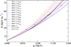 |
Fig. 1. Pressure as a function of baryonic chemical potential for both hadronic phase and quark phase. The solid lines correspond to the hadronic phase with S for which the coupling strength of S remains constant (xS = 0.03), while different values of the mass of S are supposed. The QM EOSs shown with dotted lines are characterized by two key parameters: the diquark coupling (ηD) and the vector meson coupling (ηV), respectively. The hadronic EOS without S is also shown with the dashed blue line as DD2Y-T for comparison. The colored dots show the critical chemical potential in Eq. (8) at which the RIC has been applied. |
This study aims to explore the upper limit for the mass of S as a candidate for DM within the framework of the DD2Y-T model. To determine the allowed range for the mass of S, it is important to explore the behavior of matter at high densities and make sure the results agree with the observational constraints from NSs. It is essential to note that a mass shift of S particles, xS, serves the purpose of mimicking the interaction with the surrounding medium. Given the postulation that S is a candidate for DM, it is reasonable to anticipate a predominantly weak interaction with the medium. Moore & Slatyer (2024) emphasized that for S particles to be a major DM candidate, their interactions must be extremely suppressed. Consequently, even though increasing the mass of S would inherently enable us to increase the value of xS based on our previous study (Shahrbaf et al. 2022), it is a deliberate choice to maintain xS as the coupling strength of the DM interaction with BM at its minimal value, specifically xS = 0.03 throughout the subsequent analyses. Although the chosen value of xS is small, Eq. (3) shows that increasing the baryon density still leads to a significant ΔmS, effectively mimicking the interactions between DM and BM in the dense cores of NSs. This simplifying approach allows us to systematically vary the mass of the DM candidate and examine its impact on the consistency of the hybrid star EOS, which includes hyperons in the hadronic phase, with current observational constraints.
Therefore, we applied RIC, as outlined in Section 2.3, to model the phase transition from hadronic matter to deconfined QM. Within this approach, we studied the influence of the mass of S particles on the hybrid EOS and aim to determine the maximum allowed value for the mass of S.
Figure 1 illustrates the pressure as a function of the baryonic chemical potential, showcasing both the hadronic phase and the quark phase. In the context of the hadronic phase, the coupling strength of S remains constant, as previously discussed, while different values of the mass of S with an increasing trend are supposed. One should notice that in comparison to the hadronic EOS without S (as represented by DD2Y-T, which includes nucleons and hyperons), the inclusion of S as a DM candidate results in an obvious softening of the EOS, although a repulsive interaction between DM and BM is considered. In the quark phase, we depict two various EOSs with specific parameters determined through BA, as outlined in reference Shahrbaf et al. (2023). Among the posterior-favored nlNJL parametrizations, we specifically select those that yield the earliest possible phase transition when combined with each hadronic EOS. This conservative choice ensures that deconfinement sets in as early as allowed by the model. Without this criterion, each hadronic EOS could, in principle, intersect with several different QM curves, leading to multiple possible transition points.
The color dots show the crossing point between hadronic and quark lines, where the RIC with a negative value of ΔP in Eq. (9) has been applied to correct the mischaracterization of a transition from hadronic matter to deconfined QM. As a result, at lower densities, the hadronic phase dominates, while at high densities, the quark phase remains a valid description. One should also point out that the RIC construction with ΔP < 0 generates a peak in the squared speed of sound (as shown in Fig. 11 of Shahrbaf et al. (2022)), consistent with the phenomenologically established behavior observed in QCD-based studies.
It is important to emphasize again that, for each hadronic EOS, we have selected the first intersection point with the QM EOS as the basis for implementing the phase transition construction. Although the two QM EOSs used in this study differ only slightly in stiffness, the softest three hadronic EOSs, corresponding to mS= 1890, 1895, and 1900 MeV, do not intersect with the stiffer of the two quark EOSs. Therefore, in the next section, where we perform a detailed scan over the mass of the S particle, these three soft hadronic models are combined with the first QM EOS (characterized by ηD = 0.70, ηV = 0.10). The remaining hadronic models are matched with the second, slightly stiffer QM EOS (with ηD = 0.70, ηV = 0.11). For both parametrizations, the squared speed of sound is inferred to be cs2 = 0.44.
It can be seen that increasing the mass of S leads to a noticeable stiffening of the hadronic EOS. As a result, the crossing point between the hadronic and QM EOS curves shifts toward higher values of the baryonic chemical potential, and consequently, to higher baryonic densities. This shift in the onset of the deconfinement transition has important implications for the internal structure of the star in the hadronic phase, influencing both the density profile and the composition of matter, including the presence and population of hadronic and exotic particles.
In Fig. 2, we illustrate how a RIC construction is performed between the hadronic EOS – represented by DD2Y-T+S1900, which includes nucleons, hyperons, and a S with mS = 1900 MeV – and the QM EOS described by the nlNJL model with parameters ηD = 0.70, ηV = 0.10. The crossover phase transition between the two phases is characterized by a negative value of ΔP. The matching points defined earlier as μH and μQ, representing the chemical potentials at which the pressure of the crossover phase is in accordance with the pressures of the hadronic and QM phases, are clearly illustrated in the figure. This figure shows how a negative value for ΔP in the context of RIC effectively addresses the issue of a nonphysical intersection point, often referred to as the reconfinement point. This adjustment restores the hadronic phase at lower densities and the QM phase at higher densities. In contrast to our assumption, the inverted or cross hybrid star scenarios (Zhang & Ren 2023; Zhang et al. 2024; Negreiros et al. 2025) assume that QM can be absolutely stable at low densities (low pressure), allowing for hadronic cores surrounded by QM layers. These approaches represent complementary assumptions, and future high-precision astrophysical observations will be crucial to determine which scenario, if either, is realized in nature.
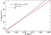 |
Fig. 2. Pressure as a function of baryonic chemical potential for the hadronic phase, QM phase, and the hybrid EOS constructed within the framework of RIC for mS = 1900 MeV. |
Figure 3, shows the pressure as a function of energy density for the baseline hadronic EOSs (DD2 and DD2Y-T) and the constructed hybrid EOSs. All employed and constructed EOSs are consistent with the (Hebeler et al. 2013) constraint (yellow region) and largely fall within the narrower (Miller et al. 2021) region (between dashed green lines), with only slight deviations at higher S-particle masses. At low energy densities, where hadronic matter dominates, the hybrid EOSs with DM are softer than the reference hadronic lines (DD2: black dash-dotted, DD2Y-T: light red lines) and also the hybrid RIC-DD2Y-T (violet) line, with stiffness increasing for higher S masses. At high energy densities, where QM governs, all hybrid EOSs converge, as both quark EOS sets share the same stiffness and speed of sound, rendering the high-density behavior almost insensitive to the S DM mass. At this region, the hybrid EOSs with DM (RIC-DD2Y-T+S) remain softer than DD2 but stiffer than DD2Y-T and RIC-DD2Y-T.
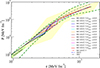 |
Fig. 3. Pressure as a function of energy density for the baseline hadronic EOSs (DD2 and DD2Y-T) and the constructed hybrid EOSs. The yellow shaded region and dashed green line indicate the constraints from Hebeler et al. (2013) and Miller et al. (2021), respectively. |
Regarding the production of S particles inside the hybrid star modeled by the approach described above, Fig. 4 shows the variation of the DM particle fraction as a function of baryon number density for different S-particle masses. In general, lighter S particles result in a higher DM fraction at a given density. Increasing the mass of S shifts the DM onset to higher densities, leading to a smaller fraction of heavier S particles being produced in stellar matter. For a fixed S mass, the DM fraction increases as the system becomes denser. However, at high densities, around nB ≈ 1fm−3, the DM fraction becomes roughly the same across all considered S masses shown in the legend. The vertical black and dash-dotted red lines indicate the deconfinement onset densities, corresponding to μH for mS = 1890 MeV and mS = 2054 MeV, respectively, marking the chemical potentials at which some degrees of phase transition to QM occur. It is worth noting that the microscopic evolution of particle fractions within the mixed phase is not explicitly determined in our approach. The onset of the transition is specified by μH, and the maximum DM fraction is reached at this threshold density for each stellar mass. Consequently, the maximum DM fraction allowed in our models varies from about 12% for the highest S-particle mass to 15% for the lightest one. Although the DM fractions vary along the curves, from zero up to about 30% at very high densities within the pure hadronic phase, the maximum S fraction inside hybrid stars changes only within a narrow range of 12–15%. This behavior indicates that increasing the DM particle mass not only shifts the DM onset to higher densities but also delays the deconfinement transition, pushing it to even higher densities, as also seen in Fig. 1.
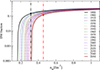 |
Fig. 4. Fraction of S particles as a DM candidate in the hadronic phase calculated using the DD2Y-T model for various S particle masses. The fractions are shown from the respective onset densities up to densities beyond the central density of NSs, illustrating how the S fraction evolves within the purely hadronic phase. The black and red dash-dotted lines indicate the onset densities for the transition to deconfined QM, corresponding to μH for mS = 1890 MeV and mS = 2054 MeV, respectively. |
4. Neutron star constraints on the mass of dark matter particles
As explained in the previous sections, recent multimessenger observations of NSs offer a valuable chance to explore the structure of high-density matter, which may contain exotic components such as hyperons, QM, or even DM. In this section, based on the astrophysical constraints of NSs, we investigate our hybrid EOS and determine the allowed maximum mass for the S particle. For this purpose, the latest M-R measurements by NICER telescope have been applied, which provide reliable constraints for the radius of NSs with masses around 2 M⊙ and 1.4 M⊙ (Miller et al. 2019; Riley et al. 2019; Miller et al. 2021; Riley et al. 2021; Choudhury et al. 2024a; Mauviard et al. 2025b). Since all of our hybrid EOSs pass well through the center of the NICER constraint region for PSR J0740+6620 with a mass of 2 M⊙, we now focus primarily on the most recent results for the pulsars PSR J0614–3329 which has a measured mass of  and radius
  (Mauviard et al. 2025b), and PSR J0437–4715 (M = 1.418 ± 0.037 M⊙,
  ) (Choudhury et al. 2024a).
Furthermore, tidal deformability, which describes how a NS deforms under the gravitational influence of its companion in a binary system, is also taken into account. This parameter is highly sensitive to the EOS and the compactness of the star (Hinderer 2008; Hinderer et al. 2010). We therefore examined whether our hybrid model aligns with the tidal deformability constraint for a 1.4 M⊙ NS, given as  (Abbott et al. 2018).
In addition, since our model incorporates several important degrees of freedom in dense matter, including hyperons, DM, and the phase transition to deconfined QM, we include recent exotic mass measurements of NSs for a more comprehensive analysis. Specifically, we consider HESS J1731–347 as the lowest-mass known NS (Doroshenko et al. 2023), and PSR J0952–0607, the BW pulsar, as the highest-mass candidate (Romani et al. 2022).
To evaluate the reliability of our model and explore how the DM parameters align with observational constraints on NS properties, both the pure hadronic and hybrid EOSs are used as inputs to the Tolman–Oppenheimer–Volkoff equations (Tolman 1939; Oppenheimer & Volkoff 1939). This allows us to obtain the M–R relations corresponding to each EOS. The results are displayed in Fig. 5, where the observational M–R constraints are shown as color-coded regions for comparison.
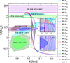 |
Fig. 5. Mass-radius relations for NSs with a purely hadronic core (dashed blue line), hybrid stars without DM (dash-dotted red line), and hybrid stars including DM for different S particle masses (solid colored lines). The colored regions represent observational constraints for comparison. The 1-σ M-R constraint from the NICER analysis of PSR J0740+6620 is shown in turquoise (Dittmann et al. 2024b). The updated 95% and 68% credible NICER results for PSR J0030+0451 are displayed as nested light and dark cyan regions (Vinciguerra et al. 2023). The hatched magenta and green regions show the high-mass BW pulsar PSR J0952-0607 (Romani et al. 2022) and PSR J0348+0432 (Antoniadis et al. 2013), respectively. The credible intervals for HESS J1731-347 are shown as nested green regions, representing the 68% (inner) and 90% (outer) levels based on X-ray spectral modeling (Doroshenko et al. 2023). The M-R constraints for PSR J0437-4715 are represented by overlapping dark and light blue regions, corresponding to the 68% (inner) and 90% (outer) credible intervals (Choudhury et al. 2024a). The nested light and dark maroon regions show the most recent NICER analysis for the mass and radius of PSR J0614-3329, 95% and 68% credible results, respectively (Mauviard et al. 2025a). The zoomed-in region (a) highlights that all RIC EOSs including S DM pass through the 95% credible region of PSR J0614–3329, whereas the RIC_DD2Y-T and DD2Y-T curves do not satisfy this constraint. The zoomed-in region (b) illustrates that for S masses larger than 1930 MeV, the NS radius lies outside the 68% credible region for PSR J0437–4715. |
In Fig. 5, the M–R curve for the pure hadronic EOS, which includes hyperons (DD2Y-T), is shown with a dashed blue line. The dash-dotted red line represents the hybrid EOS without any DM (S) particles (RIC_DD2Y-T). The solid colored lines show the full hybrid model that includes hyperons, S particles, and QM, where each color corresponds to a different S mass as indicated in the legend.
From the M–R curves, we can see that increasing the mass of S particles shifts the phase transition to QM to higher densities, meaning it happens at higher NS masses. This can be observed from the point where the curves start to deviate from the pure hadronic one. Because of the production of DM particles and the resulting softening, the radius of the star changes compared to the model without S, bringing the results in better agreement with all the observational constraints. The softening induced by DM acts mainly in the hadronic phase, which reduces radii at ∼1.4 M⊙. By contrast, the maximum mass is governed predominantly by the high-density quark EOS, which is essentially unchanged across our cases because both quark-matter parametrizations result in the same cs2. Consequently, the hybrid EOSs with DM yield comparable Mmax. The onset density of the phase transition also matters. For example, the RIC-DD2Y-T EOS (without DM) has a late transition, retains a larger hadronic fraction at high density, and therefore attains a smaller Mmax. While all S masses satisfy the high-mass limit, the region corresponding to HESS J1731–347 is only consistent with the lowest S masses (mS ≲ 1900 MeV), due to the earlier deconfinement transition. The latest NICER M-R results for PSR J0614–3329, presented with maroon regions, indicate a measured mass of ∼1.4 M⊙ having a radius comparable to HESS J1731–347. As also shown in the zoomed-in panel (a), all hybrid EOSs constructed using the RIC method and including S DM are found to intersect the 95% credible region of PSR J0614-3329. In contrast, both the RIC_DD2Y-T and DD2Y-T models, which either exclude DM or represent purely hadronic matter, fail to meet this observational constraint. This highlights that the consistency of a model with such a compact object requires additional softening beyond what is provided by hyperons or QM alone. Therefore, the presence of an additional degree of freedom, such as S DM, can supply the necessary softening and make our hybrid model consistent with the most recent NICER results.
In addition, considering the NICER results for PSR J0437-4715, which also gives the allowed radius range for a 1.4 M⊙ NS, we find that including S particles shifts the curves toward the center of the nested blue regions, making the model more consistent with observations. In fact, as shown in the zoomed-in panel (b), for mS ≤ 1930 MeV, the hybrid EOSs even fall within the 68% credible region from NICER, demonstrating consistency with the highest-probability region of the observational data.
We have also used the NICER measurements for PSR J0030+0451 from Vinciguerra et al. (2024), which represent a recent update to the analysis by Riley et al. (2019). Examining the cyan regions, the impact of the S becomes evident. In contrast to the RIC_DD2Y-T and DD2Y-T models, the EOSs that include S DM successfully pass through the 68% credible region for PSR J0030+0451, indicating strong agreement with the most likely observational results. We note that our hybrid EOSs remain consistent with the NICER measurement of PSR J1231–1411 (Salmi et al. 2024a), although this object is still under debate due to its complex pulse profile; for this reason, we did not include it in our M-R diagram.
It is important to note that the presence of DM affects the onset of the phase transition compared to the RIC_DD2Y-T EOS without S. This leads to a change in the radius of the star around 1.4 M⊙, which is a key role of S particle production in making the model consistent with tidal deformability constraints, as we will discuss in the following.
Figures 6 and 7 show how the presence of S particles affects the tidal deformability of NSs. In Fig. 6, we show how the dimensionless tidal deformability, Λ, changes with the mass of the star. The vertical green line shows the observational limit for a 1.4 M⊙ NS from the GW170817 event (Abbott et al. 2018). Different lines in the plot correspond to different S particle masses, as shown in the legend.
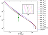 |
Fig. 6. Dimensionless tidal deformability, denoted as Λ, presented as a function of stellar mass for the ensemble of EOSs illustrated in Fig. 5. The vertical green line in the figure signifies the Λ1.4 constraint derived from the low-spin prior analysis of GW170817, as reported in (Abbott et al. 2018). |
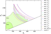 |
Fig. 7. Tidal deformability parameters Λ1 and Λ2 of the high- and low-mass components of the binary merger. The green region is the placed constraint on the tidal effects by the LIGO and Virgo collaboration from the GW170817 event (Abbott et al. 2018). |
As seen in the figure, without DM, both the pure hadronic model (DD2Y-T) and the hybrid model without S (RIC_DD2Y-T) do not meet the tidal deformability limit at 1.4 M⊙. However, adding S particles helps soften the EOS near 1.4 M⊙, which allows most hybrid models with S particles to satisfy the constraint. The zoomed-in part of the figure shows that for S masses less than about 2040 MeV, the value of Λ1.4 stays below the upper limit of 580.
For completeness, Fig. 7 shows the allowed region in the Λ1–Λ2 plane based on the GW170817 observation (Abbott et al. 2017). This figure also supports the upper limit of around 2040 MeV for the S particle mass. It can be seen that for mS ≲ 2040 MeV, the curves fall within the 90% confidence region. In contrast, for heavier S particles, as well as for the pure hadronic and hybrid models without S, the curves fall outside the allowed region.
In conclusion, based on all the available multi-messenger data from NSs, we place a limit on the maximum allowed mass of the S particle. We find that the S mass should lie between 1885 and 2040 MeV to satisfy both nuclear and astrophysical constraints. Within this range, models that include hyperons, DM, and deconfined QM can all exist in the NS core. Among them, lighter S masses around 1900 MeV are especially favored, considering the M-R data from HESS J1731–347 and PSR J0437-4715.
5. Bayesian inference from neutron star observations
To constrain the value of the S mass in our BA, we incorporated a set of astrophysical measurements leading to M–R and tidal deformability constraints presented in the previous section. Additionally, we examined the influence of individual subsets of these constraints on our EOS model estimates to assess the impact of the S mass.
5.1. Basic observational dataset
The basic dataset consists of the following
-
(I)
Precise mass measurement of PSR J0348+0432 in a white dwarf binary (Antoniadis et al. 2013):
This provides a robust lower bound on the maximum mass of NSs.
-
(II)
The NICER measurements for mass and radius for PSR J0740+6620 from Dittmann et al. (2024b), which is a recent refinement of Miller et al. (2021):

-
(III)
The NICER measurements for PSR J0030+0451 from Vinciguerra et al. (2024), which is a recent refinement of Riley et al. (2019):

-
(IV)
The mass and radius of PSR J0437-4715 (Choudhury et al. 2024b):

-
(V)
Additionally, we considered the tidal deformability constraint from the GW170817 event (Abbott et al. 2018):
These entries constitute the basic dataset employed for Bayesian inference.
5.2. Extended dataset
Additionally, we tested the results by including two extreme measurements:
-
(VI)
The high-mass BW pulsar PSR J0952-0607 (Romani et al. 2022):
-
(VII)
The low-mass ultra compact object HESS J1731-347 (Doroshenko et al. 2022):

Furthermore, we examined EOSs in light of the newly reported mass and radius measurements for the rotation-powered millisecond pulsar PSR J0614–3329, based on NICER observations, which indicate that it is a moderately massive and relatively compact object, possessing the same radius as HESS J1731–347 but nearly twice the mass:
-
(VIII)
Moderate-mass compact millisecond pulsar PSR J0614-3329 (Mauviard et al. 2025b):

5.3. Bayesian analysis framework
To determine the posterior distribution of the S mass mS given the data 𝒟, we apply Bayes’ theorem:
 (15)
(15)
assuming a uniform prior.
The total likelihood is a product over independent constraints:
 (16)
(16)
The likelihood for maximum mass constraints uses the normal cumulative distribution function:
 (17)
(17)
with μM and σM taken from measurements of the heaviest pulsars. Here F𝒩 is the cumulative normal distribution function.
For M-R constraints, we evaluated the maximum likelihood approach:
![Mathematical equation: $$ \begin{aligned} p(D_{MR}|m_{\rm S}) = \max _{\varepsilon _c}\left[ f_{MR}\left(M(\varepsilon _c), R(\varepsilon _c)\right)\right]. \end{aligned} $$](/articles/aa/full_html/2026/02/aa56315-25/aa56315-25-eq44.gif) (18)
(18)
The density functions fMR are obtained via kernel density estimation (KDE) using public datasets from Zenodo (Vinciguerra et al. 2023; Dittmann et al. 2024b; Choudhury et al. 2024a; Doroshenko et al. 2023; Mauviard et al. 2025a).
Similarly, the GW170817 constraint was evaluated as
 (19)
(19)
where fGW is the non-symmetric split normal distribution of the tidal deformability for mass 1.4 M⊙.
Finally, the Bayesian evidence was computed as
 (20)
(20)
Bayesian evidence plays two roles: a normalization factor in Bayesian inference, a measure of how well data can be explained by a model on average, considering all the parameter values it allows. We decided to provide the values of the evidences in the legends of the figures presenting our BA results, so that others can use them to calculate Bayes factors and compare their models with ours.
Note that we prefer the maximum likelihood approach over numerical marginalization, as employed, for example, in Alvarez-Castillo et al. (2016), Shahrbaf et al. (2023), Ayriyan et al. (2025), because marginalizing over central density can introduce noticeable numerical inaccuracies when the EOS stiffness varies significantly within the target region. A fixed step in central density may lead to significant uneven sampling in observable space (e.g., mass and radius) across different EOSs, potentially biasing the results. We observed this effect in the region of the most probable NS masses, where our EOS exhibits substantial variation in stiffness. In this regime, numerical marginalization using M-R constraints from Vinciguerra et al. (2023), Choudhury et al. (2024b) and Mauviard et al. (2025b) becomes less reliable for our case. In contrast, the maximum likelihood method directly identifies the best-fitting models without relying on sensitive numerical integration.
5.4. Bayesian analysis results
The resulting posterior distributions, shown in Fig. 8, reveal varying sensitivity to the different observational datasets. As seen in Fig. 8a, the 2 M⊙ constraints from the precise mass measurement of PSR J0348+0432 (Antoniadis et al. 2013) and the NICER measurement of PSR J0740+6620 (Dittmann et al. 2024b) yield a nearly uniform posterior, indicating that all considered S masses support sufficiently massive NSs. Similarly, Fig. 8c shows that the tidal deformability constraint from GW170817, calibrated at 1.4 M⊙, only mildly disfavors the highest S masses. These two results are consistent with the fact that the physical parameter space for the S mass was pre-selected to satisfy both the 2 M⊙ mass requirement and the tidal deformability bound Λ1.4. Consequently, the extremely massive BW pulsar PSR J0952–0607 (Romani et al. 2022) (see Fig. 9a) has a negligible impact on the posterior distribution as well.
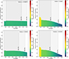 |
Fig. 8. Posterior distribution for different sets of constraints. (a) (I) and (II), (b) (III) and (IV), (c) (V), (d) (I)–(V). |
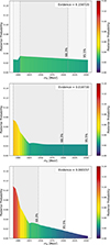 |
Fig. 9. Posterior for an additional set of constraints: (VI) high-mass BW pulsar PSR J0952-0607 (Romani et al. 2022) and (VII) ultracompact HESS J1731-347 (Doroshenko et al. 2022). (a) (VI), (b) (VII), (c) (I)–(VII). |
More discriminating behavior is observed in Fig. 8b, where NICER M–R measurements for PSR J0030+0451 (Vinciguerra et al. 2024) and PSR J0437–4715 (Choudhury et al. 2024b), both representative of canonical 1.4 M⊙ NSs, clearly favor lighter S masses (below 1930 MeV) while disfavoring the upper end of the tested range. This trend persists in Fig. 8d when combining all standard M-R and tidal deformability constraints (I)–(V). The preference for lower masses in this region reflects the requirement for an earlier onset of the phase transition to remain consistent with NICER radius measurements.
Incorporating the exotic compact objects HESS J1731–347 and PSR J0952–0607 in Fig. 9 further reinforces this trend. In particular, the lightness and high compactness of HESS J1731–347 strongly favor S masses mS ≲ 1900 MeV(Fig. 9b), while our model intersects only the higher right edge of the 95% confidence region inferred for this object by Doroshenko et al. (2022). This happens because the constraint yields a higher weighted likelihood difference for different values of mS.
It is worth noting that, due to the unexpectedly high compactness of this source, we expect that future refinements may lead to significant changes in its estimated mass and radius in favor of less compactness, despite this, various hypotheses are now being put forward about the nature of this ultracompact object. Several studies have proposed the nature of such light and ultracompact objects, it could be strange stars (Di Clemente et al. 2024; Horvath et al. 2023; Yuan & Zhou 2025), hybrid stars with a deconfined quark core (Ayriyan et al. 2025), or even third family compact stars (Ayriyan et al. 2025; Alvarez-Castillo 2025). On the basis of the obtained results, we alternatively suggest that the presence of DM in such objects is a plausible hypothesis.
The final Fig. 9c illustrates the results of the analysis including all the constraints on mass and radius (I)–(VII). The dominant contribution to the posterior distribution arises from constraints in the region of canonical masses, as well as from the ultracompact object, resulting in an even stronger preference for lower masses of S.
In the final part of the analysis, we included a recently appeared estimate of the mass and radius of the pulsar PSR J0614–3329 (Mauviard et al. 2025b), labeled as constraint (VIII). This object has a canonical mass of 1.44 M⊙ and a relatively small radius, making it a notably compact object in contrast to constraints (III) and (IV). Since these objects are assumed to have approximately the same mass, the M-R curve is expected to pass through the region where the uncertainties of these constraints overlap, this is satisfied primarily for lower S masses. The results shown in Fig. 10a indicate that the influence of this new constraint on the posterior distribution of the DM particle mass is similar to that of constraints (III) and (IV). Its combination with the baseline constraints (I)–(V) clearly enhances the preference for low-mass S particles (see Fig. 10b). When all constraints are taken into account, this preference becomes extremely dominant, as seen in Fig. 10c.
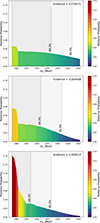 |
Fig. 10. Posterior distribution with new NICER constraints (VIII) from the millisecond pulsar PSR J0614–3329 (Mauviard et al. 2025b). (a) (VIII), (b) (I)–(V) and (VIII), (c) (I)–(VIII). |
6. Summary and conclusions
Motivated by the theoretical existence of a stable sexaquark configuration, S=uuddss, with a mass below 2054 MeV, we have explored its role as a bosonic DM candidate within the core of NSs. Using the DD2Y-T model to describe the hadronic phase, incorporating both hyperons and the sexaquark (S) as a bosonic DM component, we modeled the superconducting QM phase with the nlNJL model. A smooth crossover transition between these two phases was constructed using the RIC method. We find that hybrid configurations reach a maximum S DM fraction of about 12–15%.
Our results show that the inclusion of S particles with a weak repulsive interaction, modeled via a positive mass shift, leads to a softening of the EOS. This effect is consistent with the role of the first established hexaquark, the d*(2380), whose inclusion in the NS EOS has also been shown to soften the EOS and alter the deconfinement threshold. This softening plays a critical role in addressing the tension between stiff hadronic EOSs and tidal deformability constraints, particularly around the canonical 1.4 M⊙ mass range. In contrast to purely hadronic or hybrid models without DM, the resulting hybrid stars, comprising a deconfined QM core and a hypernuclear outer layer enriched with S DM, satisfy all current observational constraints on NS properties.
Incorporating recent astrophysical observations, we find that for mS ≤ 1935 MeV, the M-R relations of the resulting hybrid stars not only remain consistent with existing measurements but also lie within the 68% credible region from NICER for PSR J0437–4715 around 1.4 M⊙. Moreover, the hybrid star configurations with the two lowest S masses used in this work agree with the constraints inferred from the low-mass ultracompact object HESS J1731–347. For 1885 < mS < 2040 MeV, the tidal deformability Λ1.4 remains below the observational upper limit of 580, further supporting the viability of our EOS. For comparison, we note that axion-like DM is expected in the μeV-MeV range, while weakly interacting massive particles are typically considered in the GeV-TeV range. Our results constrain the S particle mass to the ∼2 GeV scale, placing it in a distinct region among DM candidates.
It is worth noting that without the presence of DM, the considered hadronic (DD2Y-T) and hybrid (RIC_DD2Y-T) models are not consistent with Λ1.4. In addition, by employing the recently updated NICER M-R results for PSR J0030+0451, we showed that the EOSs including S DM are compatible with the most probable observational values, i.e., the 68% credible region, while the hybrid model without S and the pure hadronic EOS are only consistent with the 95% region.
Furthermore, to place the most stringent constraint on the S mass while accounting for all available observational data, we have incorporated the latest NICER M-R measurements of PSR J0614–3329, which became available prior to the submission of this study. We find that, unlike the EOSs without the S component, all models that include DM favor the 95% credible region, with lighter S particles being particularly preferred. This noteworthy result provides strong support for our model in which S particles are produced inside NSs and thus coexist with other possible internal structures, including hyperons and QM.
We conclude that including S DM as an additional degree of freedom alongside hyperons and deconfined QM plays a crucial role in ensuring the consistency of the model with all available observational data. In particular, it makes the model more favorable around 1.4 M⊙, reflecting close alignment with the most robustly inferred NS properties.
To investigate the parameter space of S and constrain its mass more precisely, we performed a BA that incorporates all key observational constraints within a consistent statistical framework. This includes all available M-R measurements by the NICER telescope and the tidal deformability constraint from the GW170817 event by LIGO/Virgo detectors. Additionally, we considered two astrophysical extremes: HESS J1731–347, representing the most compact (lightest) known NS, and PSR J0952–0607, the most massive NS observed to date. These sources provide critical boundary conditions for constraining the EOS across the full density range.
To the best of our knowledge, this study incorporates all currently available and relevant observational data to evaluate the viability of the proposed model. We find that our hybrid model, comprising ordinary nuclear matter, hyperons, S bosonic DM, and deconfined QM, satisfies all observational constraints only when S DM is included. This highlights the essential role of the additional softening and thus the smaller radii around 1.4 M⊙ introduced by the S component. The Bayesian inference yields a posterior distribution that disfavors S particle masses higher than 2000 MeV (placing them outside the 95.5% credibility region) and strongly favors mS ≲ 1935 MeV (within the 68.3% credibility region), suggesting that such a DM candidate may contribute meaningfully to the dense matter composition of NSs.
While our study does not claim that the presence of S particles is required to explain NS properties, it provides compelling evidence that their inclusion leads to the improved consistency of our model with current observational data. Future observations, particularly those sensitive to the thermal and cooling behavior of NSs, may offer further insight into the role of such exotic particles in the interiors of compact stars.
We emphasize that in this work, we have focused on testing the astrophysical viability of the S particle as a DM candidate inside NSs. Our assumption of a small fixed value of xS effectively models a weak coupling to the medium and is consistent with current literature. A DM S state remains viable provided its vacuum couplings to baryons are small, while in-medium effects at sufficiently high densities can still shift its effective mass to influence the EOS. Our present results should be interpreted as the limit of equilibrium configurations. We note that a definitive assessment requires future work that (i) computes weak reaction rates and equilibration timescales involving S, (ii) implements a dynamical vector interaction for S beyond a linear mass shift, and (iii) treats possible deconfinement-driven dissociation consistently. These improvements will determine whether the equilibrium compositions assumed here are achieved on astrophysical timescales, but they lie beyond the scope of the present study.
In summary, our analysis shows that the inclusion of DM provides a viable mechanism to soften the stiff hadronic EOSs, such as DD2Y-T, enabling them to remain consistent with modern astrophysical constraints. We stress, however, that this conclusion is model dependent, as softer EOSs may not require, and could even be disfavored by, the presence of DM. In this sense, DM should be regarded as one possible solution among several proposed in the literature to reconcile current tensions between the precise measurements of high mass NSs and the existence of very compact NSs, alongside scenarios such as two families of compact stars (Drago et al. 2016; Drago & Pagliara 2016; Drago et al. 2014), slowly stable hybrid stars (Mariani et al. 2024; Laskos-Patkos & Moustakidis 2025), or scenarios involving self-bound hybrid stars and hybrid stars that remain radially stable in the context of slow (or even fast) phase transitions (Zhang et al. 2025).
As a final remark, we note that our analysis is not in contradiction with halo-like DM distributions on galactic scales. Rather, our model describes the distribution of S particles inside NSs under the assumption of non-gravitational BM-DM coupling. The shell-like configuration of S DM at the stellar level can, in principle, coexist with extended DM halo structures on larger astrophysical scales. Thus, our results are not in tension with the DM galactic halo distribution but are complementary to it, providing an additional way to probe this model through multi-messenger observations of NSs.
Acknowledgments
M. Sh. would like to thank G. Farrar and D. Blaschke, her co-authors on a previous work, for valuable discussions and correspondence that significantly contributed to her understanding of the sexaquark concept and its implications for neutron star physics. M. Sh. has been supported by NCN under SONATINA 7 grant NO. 2023/48/C/ST2/00297 and also by the program Excellence Initiative-Research University of the University of Wroclaw of the Ministry of Education and Science. D.R.K was supported by SONATINA 7 grant NO. 2023/48/C/ST2/00297. D.R.K was, in part, supported by Polish NCN Grant No. 2023/51/B/ST9/02798. A.A. was supported by NCN under grant No. 2021/43/P/ST2/03319.
References
- Abbott, B. P., Abbott, R., Abbott, T. D., et al. 2017, Phys. Rev. Lett., 119, 161101 [Google Scholar]
- Abbott, B. P., Abbott, R., Abbott, T. D., et al. 2018, Phys. Rev. Lett., 121, 161101 [Google Scholar]
- Abbott, B. P., Abbott, R., Abbott, T. D., et al. 2020, ApJ, 892, L3 [NASA ADS] [CrossRef] [Google Scholar]
- Abelev, B. I., Aggarwal, M. M., Ahammed, Z., et al. 2010, Science, 328, 58 [CrossRef] [PubMed] [Google Scholar]
- Acharya, S., Adamová, D., Adler, A., et al. 2022, Phys. Rev. Lett., 128, 252003 [CrossRef] [PubMed] [Google Scholar]
- Acharya, S., Adamová, D., Adler, A., et al. 2023, Phys. Rev. Lett., 131, 102302 [CrossRef] [PubMed] [Google Scholar]
- Adlarson, P., Adolph, C., Augustyniak, W., et al. 2011, Phys. Rev. Lett., 106, 242302 [CrossRef] [PubMed] [Google Scholar]
- Alvarez-Castillo, D. E. 2025, Universe, 11, 224 [Google Scholar]
- Alvarez-Castillo, D., Ayriyan, A., Benic, S., et al. 2016, Eur. Phys. J. A, 52, 69 [NASA ADS] [CrossRef] [Google Scholar]
- Antoniadis, J., Freire, P. C. C., Wex, N., et al. 2013, Science, 340, 6131 [Google Scholar]
- Arbey, A., & Mahmoudi, F. 2021, Prog. Part. Nucl. Phys., 119, 103865 [CrossRef] [Google Scholar]
- Arcadi, G., Dutra, M., Ghosh, P., et al. 2018, Eur. Phys. J. C, 78, 203 [NASA ADS] [CrossRef] [Google Scholar]
- Arvikar, P., Gautam, S., & Venneti, A. 2025, Phys. Rev. D, 112, 023021 [Google Scholar]
- Ávila, A., Giangrandi, E., Sagun, V., Ivanytskyi, O., & Providência, C. 2024, MNRAS, 528, 6319 [Google Scholar]
- Ayriyan, A., & Grigorian, H. 2018, EPJ Web Conf., 173, 03003 [Google Scholar]
- Ayriyan, A., Bastian, N. U., Blaschke, D., et al. 2018, Phys. Rev. C, 97, 045802 [Google Scholar]
- Ayriyan, A., Blaschke, D., Grunfeld, A. G., et al. 2021, Eur. Phys. J. A, 57, 318 [NASA ADS] [CrossRef] [Google Scholar]
- Ayriyan, A., Blaschke, D., Carlomagno, J. P., Contrera, G. A., & Grunfeld, A. G. 2025, Universe, 11, 141 [Google Scholar]
- Azizi, K., Agaev, S. S., & Sundu, H. 2020, J. Phys. G, 47, 095001 [Google Scholar]
- Barbat, M. F., Schaffner-Bielich, J., & Tolos, L. 2024, Phys. Rev. D, 110, 023013 [Google Scholar]
- Baryakhtar, M., Caputo, R., Croon, D., et al. 2022, ArXiv e-prints [arXiv:2203.07984] [Google Scholar]
- Bauswein, A., Bastian, N.-U. F., Blaschke, D. B., et al. 2019, Phys. Rev. Lett., 122, 061102 [Google Scholar]
- Bauswein, A., Blaschke, D., & Fischer, T. 2022, Effects of a strong phase transition on supernova explosions, compact stars and their mergers [Google Scholar]
- Baym, G., Hatsuda, T., Kojo, T., et al. 2018, Rept. Prog. Phys., 81, 056902 [CrossRef] [PubMed] [Google Scholar]
- Beane, S. R., Chang, E., Detmold, W., et al. 2011, Phys. Rev. Lett., 106, 162001 [Google Scholar]
- Bertone, G., & Hooper, D. 2018, Rev. Mod. Phys., 90, 045002 [NASA ADS] [CrossRef] [Google Scholar]
- Bertone, G., & Tait, M. P. T. 2018, Nature, 562, 51 [Google Scholar]
- Biesdorf, C., Schaffner-Bielich, J., & Tolos, L. 2025, Phys. Rev. D, 111, 083038 [Google Scholar]
- Blaschke, D., Ivanytskyi, O., & Shahrbaf, M. 2022, Quark deconfinement in compact stars through sexaquark condensation [Google Scholar]
- Bramante, J., & Raj, N. 2024, Phys. Rept., 1052, 1 [Google Scholar]
- Braun-Munzinger, P., Kalweit, A., Redlich, K., & Stachel, J. 2015, Phys. Lett. B, 747, 292 [CrossRef] [Google Scholar]
- Castorina, P., Redlich, K., & Satz, H. 2009, Eur. Phys. J. C, 59, 67 [CrossRef] [Google Scholar]
- Celi, M. O., Bashkanov, M., Mariani, M., et al. 2024, Phys. Rev. D, 109, 023004 [Google Scholar]
- Celi, M. O., Mariani, M., Kumar, R., et al. 2025, Phys. Rev. D, 112, 023027 [Google Scholar]
- Chadha-Day, F., Ellis, J., & Marsh, D. J. E. 2022, Sci. Adv., 8, abj3618 [Google Scholar]
- Choi, S., Hiyama, E., Hyun, C. H., & Cheoun, M. K. 2023, ArXiv e-prints [arXiv:2309.01348] [Google Scholar]
- Choudhury, D., Salmi, T., Serena, V., et al. 2024a, https://doi.org/10.5281/zenodo.13766753 [Google Scholar]
- Choudhury, D., Salmi, T., Vinciguerra, S., et al. 2024b, ApJ, 971, L20 [NASA ADS] [CrossRef] [Google Scholar]
- Christian, J.-E., Schaffner-Bielich, J., & Rosswog, S. 2024, Phys. Rev. D, 109, 063035 [Google Scholar]
- Cipriani, L., Giangrandi, E., Sagun, V., Doneva, D. D., & Yazadjiev, S. S. 2025, Phys. Rev. D, 111, 123005 [Google Scholar]
- Cirelli, M., Strumia, A., & Zupan, J. 2024, ArXiv e-prints [arXiv: 2406.01705] [Google Scholar]
- Collier, M., Croon, D., & Leane, R. K. 2022, Phys. Rev. D, 106, 123027 [Google Scholar]
- Counsell, A. R., Gittins, F., Andersson, N., & Tews, I. 2025, ArXiv e-prints [arXiv:2504.06181] [Google Scholar]
- Das, H. C., & Burgio, G. F. 2025, Universe, 11, 5 [Google Scholar]
- Das, A., Jaikumar, P., Karekkat, A., & Mandal, T. 2025, Phys. Rev. Lett., 135, 081402 [Google Scholar]
- de Martino, I., Chakrabarty, S. S., Cesare, V., et al. 2020, Universe, 6, 107 [NASA ADS] [CrossRef] [Google Scholar]
- Dengler, Y., Schaffner-Bielich, J., & Tolos, L. 2022, Phys. Rev. D, 105, 043013 [CrossRef] [Google Scholar]
- Dengler, Y., Kulkarni, S., Maas, A., & Radl, K. 2025, ArXiv e-prints [arXiv:2503.19691] [Google Scholar]
- Di Clemente, F., Drago, A., & Pagliara, G. 2024, ApJ, 967, 159 [CrossRef] [Google Scholar]
- Diedrichs, R. F., Becker, N., Jockel, C., et al. 2023, Phys. Rev. D, 108, 064009 [Google Scholar]
- Dietrich, T., Coughlin, M. W., Pang, P. T. H., et al. 2020, Science, 370, 1450 [Google Scholar]
- Dittmann, A. J., Miller, M. C., Lamb, F. K., et al. 2024b, Updated NICER PSR J0740+6620 Illinois-Maryland MCMC Samples, [Google Scholar]
- Dittmann, A. J., Miller, M. C., Lamb, F. K., et al. 2024b, ApJ, 974, 295 [NASA ADS] [CrossRef] [Google Scholar]
- Doroshenko, V., Suleimanov, V., Pühlhofer, G., & Santangelo, A. 2022, Nat. Astron., 6, 1444 [NASA ADS] [CrossRef] [Google Scholar]
- Doroshenko, V., Suleimanov, V. F., Pühlhofer, G., & Santangelo, A. 2023, https://doi.org/10.5281/zenodo.8232233 [Google Scholar]
- Doser, M., Farrar, G., & Kornakov, G. 2023, Eur. Phys. J. C, 83, 1149 [Google Scholar]
- Drago, A., & Pagliara, G. 2016, Eur. Phys. J. A, 52, 41 [Google Scholar]
- Drago, A., Lavagno, A., & Pagliara, G. 2014, Phys. Rev. D, 89, 043014 [NASA ADS] [CrossRef] [Google Scholar]
- Drago, A., Lavagno, A., Pagliara, G., & Pigato, D. 2016, Eur. Phys. J. A, 52, 40 [NASA ADS] [CrossRef] [Google Scholar]
- Eby, J., Kouvaris, C., Nielsen, N. G., & Wijewardhana, L. C. R. 2016, JHEP, 02, 028 [Google Scholar]
- Ecker, C., Gorda, T., Kurkela, A., & Rezzolla, L. 2025, Nat. Commun., 16, 1320 [Google Scholar]
- Ellis, J., Hütsi, G., Kannike, K., et al. 2018, Phys. Rev. D, 97, 123007 [CrossRef] [Google Scholar]
- Evans, N., & Ward, M. 2023, Phys. Rev. D, 108, 026018 [Google Scholar]
- Farrar, G. R. 2003, Int. J. Theor. Phys., 42, 1211 [Google Scholar]
- Farrar, G. R. 2018, ArXiv eprints [arXiv:1805.03723] [Google Scholar]
- Farrar, G. R. 2022, ArXiv eprints [arXiv:2201.01334] [Google Scholar]
- Farrar, G. R., & Wang, Z. 2023, ArXiv eprints [arXiv:2306.03123] [Google Scholar]
- Ferreira, O., & Fraga, E. S. 2023, JCAP, 04, 012 [Google Scholar]
- Fonseca, E., Cromartie, H. T., Pennucci, T. T., et al. 2021, ApJ, 915, L12 [NASA ADS] [CrossRef] [Google Scholar]
- Fujimoto, Y., Fukushima, K., & Weise, W. 2020, Phys. Rev. D, 101, 094009 [Google Scholar]
- Fujimoto, Y., Fukushima, K., Hotokezaka, K., & Kyutoku, K. 2023, Phys. Rev. Lett., 130, 091404 [NASA ADS] [CrossRef] [Google Scholar]
- Fujimoto, Y., Kojo, T., & McLerran, L. 2024, ArXiv e-prints [arXiv:2410.22758] [Google Scholar]
- Fujimoto, Y., Fukushima, K., Hotokezaka, K., & Kyutoku, K. 2025, Phys. Rev. D, 111, 063054 [Google Scholar]
- Fukushima, K., Kojo, T., & Weise, W. 2020, Phys. Rev. D, 102, 096017 [CrossRef] [Google Scholar]
- Gal, A. 2024, Phys. Lett. B, 857, 138973 [Google Scholar]
- Gholami, H., Rather, I. A., Hofmann, M., Buballa, M., & Schaffner-Bielich, J. 2025, Phys. Rev. D, 111, 103034 [Google Scholar]
- Giangrandi, E., Sagun, V., Ivanytskyi, O., Providência, C., & Dietrich, T. 2023, ApJ, 953, 115 [Google Scholar]
- Green, J. R., Hanlon, A. D., Junnarkar, P. M., & Wittig, H. 2021, Phys. Rev. Lett., 127, 242003 [CrossRef] [PubMed] [Google Scholar]
- Grippa, F., Lambiase, G., & Poddar, T. K. 2025, Universe, 11, 74 [Google Scholar]
- Gross, C., Polosa, A., Strumia, A., Urbano, A., & Xue, W. 2018, Phys. Rev. D, 98, 063005 [Google Scholar]
- Guha, A., & Sen, D. 2024, Phys. Rev. D, 109, 043038 [Google Scholar]
- Hajkarim, F., Schaffner-Bielich, J., & Tolos, L. 2024, ArXiv eprints [arXiv:2412.04585] [Google Scholar]
- Hebeler, K., Lattimer, J. M., Pethick, C. J., & Schwenk, A. 2013, ApJ, 773, 11 [CrossRef] [Google Scholar]
- Hensh, S., Huang, Y. J., Kojo, T., et al. 2025, ApJL, 991, L12 [Google Scholar]
- Hinderer, T. 2008, ApJ, 677, 1216 [NASA ADS] [CrossRef] [Google Scholar]
- Hinderer, T., Lackey, B. D., Lang, R. N., & Read, J. S. 2010, Phys. Rev. D, 81, 123016 [NASA ADS] [CrossRef] [Google Scholar]
- Hirono, Y., & Tanizaki, Y. 2019, Phys. Rev. Lett., 122, 212001 [Google Scholar]
- Horvath, J. E., Rocha, L. S., de Sá, L. M., et al. 2023, A&A, 672, L11 [NASA ADS] [CrossRef] [EDP Sciences] [Google Scholar]
- Huang, C., & Sourav, S. 2025, ApJ, 983, 17 [Google Scholar]
- Inoue, T., Ishii, N., Aoki, S., et al. 2011, Phys. Rev. Lett., 106, 162002 [Google Scholar]
- Issifu, A., Thakur, P., da Silva, F. M., et al. 2025, Phys. Rev. D, 111, 083026 [Google Scholar]
- Ivanytskyi, O., Sagun, V., & Lopes, I. 2020, Phys. Rev. D, 102, 063028 [Google Scholar]
- Jaffe, R. L. 1977, Phys. Rev. Lett., 38, 195 [CrossRef] [Google Scholar]
- Jangal, F. M., Moshfegh, H. R., & Azizi, K. 2025, Eur. Phys. J. C, 85, 691 [Google Scholar]
- Kaplinghat, M., Tulin, S., & Yu, H.-B. 2016, Phys. Rev. Lett., 116, 041302 [NASA ADS] [CrossRef] [Google Scholar]
- Karkevandi, D. R., Shakeri, S., Sagun, V., & Ivanytskyi, O. 2022, Phys. Rev. D, 105, 023001 [CrossRef] [Google Scholar]
- Karkevandi, D. R., Shahrbaf, M., Shakeri, S., & Typel, S. 2024, Particles, 7, 201 [Google Scholar]
- Klangburam, T., & Pongkitivanichkul, C. 2025, Phys. Rev. D, 111, 103031 [Google Scholar]
- Kodama, N., Oka, M., & Hatsuda, T. 1994, Nucl. Phys. A, 580, 445 [Google Scholar]
- Kojo, T. 2021, AAPPS Bull., 31, 11 [CrossRef] [Google Scholar]
- Kojo, T. 2024, ArXiv e-prints [arXiv:2412.20442] [Google Scholar]
- Kojo, T., & Suenaga, D. 2022, Phys. Rev. D, 105, 076001 [Google Scholar]
- Konstantinou, A. 2024, ApJ, 968, 83 [Google Scholar]
- Kumar, A., & Sotani, H. 2025, Phys. Rev. D, 111, 043016 [Google Scholar]
- Largani, N. K., Fischer, T., Shibagaki, S., Cerdá-Durán, P., & Torres-Forné, A. 2024, A&A, 687, A245 [NASA ADS] [CrossRef] [EDP Sciences] [Google Scholar]
- Laskos-Patkos, P., & Moustakidis, C. C. 2025, Phys. Rev. D, 111, 063058 [Google Scholar]
- Lenzi, C. H., Dutra, M., Lourenço, O., Lopes, L. L., & Menezes, D. P. 2023, Eur. Phys. J. C, 83, 266 [Google Scholar]
- Leung, Y.-H. 2022, EPJ Web Conf., 259, 08001 [Google Scholar]
- Li, J. J., & Sedrakian, A. 2023, Phys. Lett. B, 844, 138062 [Google Scholar]
- Li, J. J., Sedrakian, A., & Alford, M. 2023, ApJ, 944, 206 [Google Scholar]
- Li, J. J., Sedrakian, A., & Alford, M. 2025, JCAP, 02, 002 [Google Scholar]
- Liebling, S. L., & Palenzuela, C. 2023, Liv. Rev. Rel., 26, 1 [Google Scholar]
- Lindblom, L., Lewis, S. M., & Weber, F. 2025, Phys. Rev. D, 111, 123035 [Google Scholar]
- Liu, H. M., Chu, P. C., Liu, H., Li, X. H., & Li, Z. H. 2025a, ArXiv e-prints [arXiv:2501.04382] [Google Scholar]
- Liu, X. Z., Mahapatra, P., Huang, C., et al. 2025b, Phys. Rev. D, 112, 083032 [Google Scholar]
- Lopes, L. L., & Issifu, A. 2025, Phys. Dark Univ., 48, 101922 [Google Scholar]
- Magas, V., & Satz, H. 2003, Eur. Phys. J. C, 32, 115 [CrossRef] [Google Scholar]
- Marczenko, M., McLerran, L., Redlich, K., & Sasaki, C. 2023, Phys. Rev. C, 107, 025802 [CrossRef] [Google Scholar]
- Mariani, M., Ranea-Sandoval, I. F., Lugones, G., & Orsaria, M. G. 2024, Phys. Rev. D, 110, 043026 [Google Scholar]
- Marsh, D. J. E. 2016, Phys. Rept., 643, 1 [NASA ADS] [CrossRef] [Google Scholar]
- Marzola, I., Rodrigues, E. H., Coelho, A. F., & Lourenço, O. 2025, Phys. Rev. D, 111, 063076 [Google Scholar]
- Maselli, A., Pnigouras, P., Nielsen, N. G., Kouvaris, C., & Kokkotas, K. D. 2017, Phys. Rev. D, 96, 023005 [Google Scholar]
- Maslov, K., Kolomeitsev, E., & Voskresensky, D. 2015, Phys. Lett. B, 748, 369 [CrossRef] [Google Scholar]
- Mauviard, L., Guillot, S., Salmi, T., et al. 2025a, A NICER view of the 1.4 solar masses edge-on pulsar PSR J0614–3329 [Google Scholar]
- Mauviard, L., Guillot, S., Salmi, T., et al. 2025b, ApJ, 995, 60 [Google Scholar]
- Miller, M. C., Lamb, F. K., Dittmann, A. J., et al. 2019, ApJ, 887, L24 [Google Scholar]
- Miller, M. C., Lamb, F. K., Dittmann, A. J., et al. 2021, ApJ, 918, L28 [NASA ADS] [CrossRef] [Google Scholar]
- Moore, M., & Slatyer, T. R. 2024, Phys. Rev. D, 110, 023515 [Google Scholar]
- Most, E. R., Papenfort, L. J., Dexheimer, V., et al. 2019, Phys. Rev. Lett., 122, 061101 [NASA ADS] [CrossRef] [Google Scholar]
- Mukherjee, S., Aswathi, P. S., Singha, C., & Ganguly, A. 2025, ArXiv e-prints [arXiv:2506.22353] [Google Scholar]
- Narain, G., Schaffner-Bielich, J., & Mishustin, I. N. 2006, Phys. Rev. D, 74, 063003 [CrossRef] [Google Scholar]
- Negreiros, R., Zhang, C., & Xu, R. 2025, Phys. Rev. D, 111, 063026 [Google Scholar]
- Nelson, A., Reddy, S., & Zhou, D. 2019, JCAP, 07, 012 [Google Scholar]
- Oppenheimer, J. R., & Volkoff, G. M. 1939, Phys. Rev., 55, 374 [NASA ADS] [CrossRef] [Google Scholar]
- Pang, P. T. H., et al. 2023, Nat. Commun., 14, 8352 [Google Scholar]
- Peter, A. H. G., Rocha, M., Bullock, J. S., & Kaplinghat, M. 2013, MNRAS, 430, 105 [Google Scholar]
- Pitz, S. L., & Schaffner-Bielich, J. 2023, Phys. Rev. D, 108, 103043 [Google Scholar]
- Pitz, S. L., & Schaffner-Bielich, J. 2025, Phys. Rev. D, 111, 043050 [Google Scholar]
- Radzhabov, A. E., Blaschke, D., Buballa, M., & Volkov, M. K. 2011, Phys. Rev. D, 83, 116004 [Google Scholar]
- Rafiei Karkevandi, D., Shakeri, S., Sagun, V., & Ivanytskyi, O. 2021, in 16th Marcel Grossmann Meeting on Recent Developments in Theoretical and Experimental General Relativity, Astrophysics and Relativistic Field Theories [Google Scholar]
- Rappold, C., et al. 2015, Phys. Lett. B, 747, 129 [CrossRef] [Google Scholar]
- Riley, T. E., Watts, A. L., Bogdanov, S., et al. 2019, ApJ, 887, L21 [Google Scholar]
- Riley, T. E., Watts, A. L., Ray, P. S., et al. 2021, ApJ, 918, L27 [CrossRef] [Google Scholar]
- Romani, R. W., Kandel, D., Filippenko, A. V., Brink, T. G., & Zheng, W. 2022, ApJ, 934, L17 [NASA ADS] [CrossRef] [Google Scholar]
- Routaray, P., Parmar, V., Das, H. C., et al. 2025, Phys. Rev. D, 111, 103045 [Google Scholar]
- Rutherford, N., Raaijmakers, G., Prescod-Weinstein, C., & Watts, A. 2023, Phys. Rev. D, 107, 103051 [CrossRef] [Google Scholar]
- Rutherford, N., Prescod-Weinstein, C., & Watts, A. 2025, Phys. Rev. D, 111, 123034 [Google Scholar]
- Ryan, M., & Radice, D. 2022, Phys. Rev. D, 105, 115034 [Google Scholar]
- Sagun, V., Giangrandi, E., Dietrich, T., et al. 2023, ApJ, 958, 49 [Google Scholar]
- Salmi, T., Deneva, J. S., Ray, P. S., et al. 2024a, ApJ, 976, 58 [Google Scholar]
- Salmi, T., Choudhury, D., Kini, Y., et al. 2024b, ApJ, 974, 294 [NASA ADS] [CrossRef] [Google Scholar]
- Salucci, P., Esposito, G., Lambiase, G., et al. 2021, Front. in Phys., 8, 603190 [Google Scholar]
- Satz, H. 1998, Nucl. Phys. A, 642, 130 [Google Scholar]
- Schäfer, T., & Wilczek, F. 1999, Phys. Rev. Lett., 82, 3956 [Google Scholar]
- Scordino, D., & Bombaci, I. 2025, JHEAp, 45, 371 [Google Scholar]
- Sedaghat, J., Bordbar, G. H., Haghighat, M., & Zebarjad, S. M. 2025, Eur. Phys. J. C, 85, 283 [Google Scholar]
- Sedrakian, A. 2016, Phys. Rev. D, 93, 065044 [Google Scholar]
- Sedrakian, A. 2019, Phys. Rev. D, 99, 043011 [Google Scholar]
- Sedrakian, A., Weber, F., & Li, J. J. 2020, Phys. Rev. D, 102, 041301 [Google Scholar]
- Shahrbaf, M. 2023, J. Phys. Conf. Ser., 2536, 012001 [Google Scholar]
- Shahrbaf, M., & Moshfegh, H. R. 2019, Ann. Phys., 402, 66 [Google Scholar]
- Shahrbaf, M., Blaschke, D., Grunfeld, A. G., & Moshfegh, H. R. 2020a, Phys. Rev. C, 101, 025807 [Google Scholar]
- Shahrbaf, M., Blaschke, D., & Khanmohamadi, S. 2020b, J. Phys. G, 47, 115201 [Google Scholar]
- Shahrbaf, M., Blaschke, D., Typel, S., Farrar, G. R., & Alvarez-Castillo, D. E. 2022, Phys. Rev. D, 105, 103005 [Google Scholar]
- Shahrbaf, M., Antić, S., Ayriyan, A., Blaschke, D., & Grunfeld, A. G. 2023, Phys. Rev. D, 107, 054011 [Google Scholar]
- Shakeri, S., & Hajkarim, F. 2023, JCAP, 04, 017 [Google Scholar]
- Shakeri, S., & Karkevandi, D. R. 2024, Phys. Rev. D, 109, 043029 [Google Scholar]
- Shanahan, P. E., Thomas, A. W., & Young, R. D. 2011, Phys. Rev. Lett., 107, 092004 [Google Scholar]
- Shawqi, S., & Morsink, S. M. 2024, ApJ, 975, 123 [Google Scholar]
- Shirke, S., Ghosh, S., Chatterjee, D., Sagunski, L., & Schaffner-Bielich, J. 2023, JCAP, 12, 008 [Google Scholar]
- Shirke, S., Pradhan, B. K., Chatterjee, D., Sagunski, L., & Schaffner-Bielich, J. 2024, Phys. Rev. D, 110, 063025 [Google Scholar]
- Spergel, D. N., & Steinhardt, P. J. 2000, Phys. Rev. Lett., 84, 3760 [NASA ADS] [CrossRef] [Google Scholar]
- Stone, J. R., Dexheimer, V., Guichon, P. A. M., Thomas, A. W., & Typel, S. 2021, MNRAS, 502, 3476 [CrossRef] [Google Scholar]
- Takahashi, H., Ahn, J. K., Akikawa, H., et al. 2001, Phys. Rev. Lett., 87, 212502 [CrossRef] [PubMed] [Google Scholar]
- Thakur, P., Malik, T., Das, A., Jha, T. K., & Providência, C. 2024, Phys. Rev. D, 109, 043030 [Google Scholar]
- Thakur, P., Malik, T., Das, A., et al. 2025, A&A, 697, A220 [NASA ADS] [CrossRef] [EDP Sciences] [Google Scholar]
- Tolman, R. C. 1939, Phys. Rev., 55, 364 [NASA ADS] [CrossRef] [Google Scholar]
- Tolos, L. 2025, EPJ Web Conf., 316, 01009 [Google Scholar]
- Tong, H., Elhatisari, S., & Meißner, U.-G. 2025, ApJ, 982, 164 [Google Scholar]
- Tsiopelas, S., Sedrakian, A., & Oertel, M. 2024, Eur. Phys. J. A, 60, 127 [Google Scholar]
- Typel, S. 2005, Phys. Rev. C, 71, 064301 [CrossRef] [Google Scholar]
- Typel, S., & Shlomo, S. 2024, Eur. Phys. J. A, 60, 236 [Google Scholar]
- Typel, S., & Wolter, H. H. 1999, Nucl. Phys. A, 656, 331 [Google Scholar]
- Typel, S., Ropke, G., Klahn, T., Blaschke, D., & Wolter, H. H. 2010, Phys. Rev. C, 81, 015803 [Google Scholar]
- Vidaña, I., Bashkanov, M., Watts, D. P., & Pastore, A. 2018, Phys. Lett. B, 781, 112 [Google Scholar]
- Vikiaris, M., Petousis, V., Veselsky, M., & Moustakidis, C. C. 2024, Phys. Rev. D, 109, 123006 [CrossRef] [Google Scholar]
- Vinciguerra, S., Salmi, T., Watts, A. L., et al. 2023, An updated mass-radius analysis of the 2017–2018 NICER data set of PSR J0030+0451 [Google Scholar]
- Vinciguerra, S., Salmi, T., Watts, A. L., et al. 2024, ApJ, 961, 62 [NASA ADS] [CrossRef] [Google Scholar]
- Visinelli, L. 2021, Int. J. Mod. Phys. D, 30, 2130006 [Google Scholar]
- Visinelli, L., Baum, S., Redondo, J., Freese, K., & Wilczek, F. 2018, Phys. Lett. B, 777, 64 [NASA ADS] [CrossRef] [Google Scholar]
- Weih, L. R., Hanauske, M., & Rezzolla, L. 2020, Phys. Rev. Lett., 124, 171103 [NASA ADS] [CrossRef] [Google Scholar]
- Yang, S. H., & Pi, C. M. 2024, JCAP, 09, 052 [Google Scholar]
- Yang, S.-H., Pi, C.-M., & Weber, F. 2025, Phys. Rev. D, 111, 043037 [Google Scholar]
- Yuan, Y.-J., & Zhou, X. 2025, Res. Astron. Astrophys., 25, 055016 [Google Scholar]
- Zhang, C., & Ren, J. 2023, Phys. Rev. D, 108, 063012 [Google Scholar]
- Zhang, C., Luo, Y., Li, H.-B., Shao, L., & Xu, R. 2024, Phys. Rev. D, 109, 063020 [Google Scholar]
- Zhang, C., Pretel, J. M. Z., & Xu, R. 2025, ArXiv e-prints [arXiv:2507.01371] [Google Scholar]
All Figures
|
Fig. 1. Pressure as a function of baryonic chemical potential for both hadronic phase and quark phase. The solid lines correspond to the hadronic phase with S for which the coupling strength of S remains constant (xS = 0.03), while different values of the mass of S are supposed. The QM EOSs shown with dotted lines are characterized by two key parameters: the diquark coupling (ηD) and the vector meson coupling (ηV), respectively. The hadronic EOS without S is also shown with the dashed blue line as DD2Y-T for comparison. The colored dots show the critical chemical potential in Eq. (8) at which the RIC has been applied. |
| In the text | |
|
Fig. 2. Pressure as a function of baryonic chemical potential for the hadronic phase, QM phase, and the hybrid EOS constructed within the framework of RIC for mS = 1900 MeV. |
| In the text | |
|
Fig. 3. Pressure as a function of energy density for the baseline hadronic EOSs (DD2 and DD2Y-T) and the constructed hybrid EOSs. The yellow shaded region and dashed green line indicate the constraints from Hebeler et al. (2013) and Miller et al. (2021), respectively. |
| In the text | |
|
Fig. 4. Fraction of S particles as a DM candidate in the hadronic phase calculated using the DD2Y-T model for various S particle masses. The fractions are shown from the respective onset densities up to densities beyond the central density of NSs, illustrating how the S fraction evolves within the purely hadronic phase. The black and red dash-dotted lines indicate the onset densities for the transition to deconfined QM, corresponding to μH for mS = 1890 MeV and mS = 2054 MeV, respectively. |
| In the text | |
|
Fig. 5. Mass-radius relations for NSs with a purely hadronic core (dashed blue line), hybrid stars without DM (dash-dotted red line), and hybrid stars including DM for different S particle masses (solid colored lines). The colored regions represent observational constraints for comparison. The 1-σ M-R constraint from the NICER analysis of PSR J0740+6620 is shown in turquoise (Dittmann et al. 2024b). The updated 95% and 68% credible NICER results for PSR J0030+0451 are displayed as nested light and dark cyan regions (Vinciguerra et al. 2023). The hatched magenta and green regions show the high-mass BW pulsar PSR J0952-0607 (Romani et al. 2022) and PSR J0348+0432 (Antoniadis et al. 2013), respectively. The credible intervals for HESS J1731-347 are shown as nested green regions, representing the 68% (inner) and 90% (outer) levels based on X-ray spectral modeling (Doroshenko et al. 2023). The M-R constraints for PSR J0437-4715 are represented by overlapping dark and light blue regions, corresponding to the 68% (inner) and 90% (outer) credible intervals (Choudhury et al. 2024a). The nested light and dark maroon regions show the most recent NICER analysis for the mass and radius of PSR J0614-3329, 95% and 68% credible results, respectively (Mauviard et al. 2025a). The zoomed-in region (a) highlights that all RIC EOSs including S DM pass through the 95% credible region of PSR J0614–3329, whereas the RIC_DD2Y-T and DD2Y-T curves do not satisfy this constraint. The zoomed-in region (b) illustrates that for S masses larger than 1930 MeV, the NS radius lies outside the 68% credible region for PSR J0437–4715. |
| In the text | |
|
Fig. 6. Dimensionless tidal deformability, denoted as Λ, presented as a function of stellar mass for the ensemble of EOSs illustrated in Fig. 5. The vertical green line in the figure signifies the Λ1.4 constraint derived from the low-spin prior analysis of GW170817, as reported in (Abbott et al. 2018). |
| In the text | |
|
Fig. 7. Tidal deformability parameters Λ1 and Λ2 of the high- and low-mass components of the binary merger. The green region is the placed constraint on the tidal effects by the LIGO and Virgo collaboration from the GW170817 event (Abbott et al. 2018). |
| In the text | |
|
Fig. 8. Posterior distribution for different sets of constraints. (a) (I) and (II), (b) (III) and (IV), (c) (V), (d) (I)–(V). |
| In the text | |
|
Fig. 9. Posterior for an additional set of constraints: (VI) high-mass BW pulsar PSR J0952-0607 (Romani et al. 2022) and (VII) ultracompact HESS J1731-347 (Doroshenko et al. 2022). (a) (VI), (b) (VII), (c) (I)–(VII). |
| In the text | |
|
Fig. 10. Posterior distribution with new NICER constraints (VIII) from the millisecond pulsar PSR J0614–3329 (Mauviard et al. 2025b). (a) (VIII), (b) (I)–(V) and (VIII), (c) (I)–(VIII). |
| In the text | |
Current usage metrics show cumulative count of Article Views (full-text article views including HTML views, PDF and ePub downloads, according to the available data) and Abstracts Views on Vision4Press platform.
Data correspond to usage on the plateform after 2015. The current usage metrics is available 48-96 hours after online publication and is updated daily on week days.
Initial download of the metrics may take a while.