| Issue |
A&A
Volume 706, February 2026
|
|
|---|---|---|
| Article Number | A270 | |
| Number of page(s) | 21 | |
| Section | Cosmology (including clusters of galaxies) | |
| DOI | https://doi.org/10.1051/0004-6361/202556411 | |
| Published online | 17 February 2026 | |
TDCOSMO
XXIII. Measurement of the Hubble constant from the doubly lensed quasar HE 1104−1805
1
Research Center for the Early Universe, Graduate School of Science, The University of Tokyo, 7-3-1 Hongo Bunkyo-ku Tokyo 113-0033, Japan
2
Institute of Physics, Laboratory of Astrophysics, Ecole Polytechnique Fédérale de Lausanne (EPFL), Observatoire de Sauverny 1290 Versoix, Switzerland
3
Institut de Ciències del Cosmos (ICCUB), Universitat de Barcelona (IEEC-UB) Martí i Franquès 1 08028 Barcelona, Spain
4
Institució Catalana de Recerca i Estudis Avançats (ICREA) Passeig de Lluís Companys 23 08010 Barcelona, Spain
5
Department of Physics and Astronomy, UC Davis 1 Shields Ave. Davis CA 95616, USA
6
Technical University of Munich, TUM School of Natural Sciences, Physics Department James-Franck-Straße 1 85748 Garching, Germany
7
Max-Planck-Institut für Astrophysik Karl-Schwarzschild Straße 1 85748 Garching, Germany
8
Institute for Particle Physics and Astrophysics, ETH Zurich Wolfgang-Pauli-Strasse 27 CH-8093 Zurich, Switzerland
9
STAR Institute, Liège Université, Quartier Agora – Allée du six Août 19c B-4000 Liège, Belgium
10
Department of Physics and Astronomy, University of California Los Angeles CA 90095, USA
11
Department of Physics and Astronomy, Stony Brook University Stony Brook NY 11794, USA
12
Fermi National Accelerator Laboratory PO Box 500 Batavia IL 60510, USA
13
Department of Astronomy & Astrophysics, University of Chicago Chicago IL 60637, USA
14
Sub-Department of Astrophysics, Department of Physics, University of Oxford, Denys Wilkinson Building Keble Road Oxford OX1 3RH, UK
15
European Southern Observatory Alonso de Córdova 3107 Vitacura Santiago, Chile
16
Oskar Klein Centre, Department of Physics, Stockholm University SE-106 91 Stockholm, Sweden
17
Kavli Institute for Cosmological Physics, University of Chicago Chicago IL 60637, USA
18
Center for Astronomy, Space Science and Astrophysics, Independent University Bangladesh Dhaka 1229, Bangladesh
19
Cosmic Dawn Center (DAWN), Niels Bohr Institute, University of Copenhagen Jagtvej 128 DK-2200 Copenhagen N, Denmark
20
Instituto de Fìsica y Astronomía, Universidad de Valparaíso Av. Gran Bretaña 1111 Playa Ancha Valparaíso, Chile
21
Department of Astronomy, School of Physics and Astronomy, Shanghai Jiao Tong University Shanghai 200240, China
22
Shanghai Key Laboratory for Particle Physics and Cosmology, Shanghai Jiao Tong University Shanghai 200240, China
23
Key Laboratory for Particle Physics, Astrophysics and Cosmology, Ministry of Education, Shanghai Jiao Tong University Shanghai 200240, China
★ Corresponding author: This email address is being protected from spambots. You need JavaScript enabled to view it.
Received:
15
July
2025
Accepted:
2
December
2025
Abstract
Time-delay cosmography leverages strongly lensed quasars to measure the Universe’s current expansion rate, H0, independently from other methods. The latest TDCOSMO milestone measurement primarily used quadruply lensed quasars for their mass profile constraints. However, doubly lensed quasars, being more abundant and offering precise time delays, could expand the sample by a factor of 5, significantly advancing towards a 1% precision measurement of H0. We present the first TDCOSMO analysis of a doubly imaged source, HE 1104−1805, including the measurement of the four necessary ingredients. First, by combining 17 years of data from the SMARTS, Euler, and WFI telescopes, we measured a time delay of 176.3+11.4−10.3 days. Second, using MUSE data, we extracted stellar velocity dispersion measurements in three radial bins with 5% to 13% precision. Third, employing F160W HST imaging for lens modelling and marginalising over various modelling choices, we measured the Fermat potential difference between the images. Fourth, using wide-field imaging, we measured the convergence added by objects not included in the lens modelling. By combining these four ingredients, we measured the time delay distance and the angular diameter distance to the deflector, favouring a power-law mass model over a baryonic and dark matter composite model. The measurement was performed blindly to prevent experimenter bias and resulted in a Hubble constant of H0 = +5.8−5.0 × λint km s−1Mpc−1, where λint is the internal mass sheet degeneracy parameter. This is in agreement with the TDCOSMO-2025 milestone and its precision for λint = 1 is comparable to that obtained with the best-observed quadruply lensed quasars (4–6%). This work is a stepping stone towards a precise measurement of H0 using a large sample of doubly lensed quasars, supplementing the current sample. The next TDCOSMO milestone paper will include this system in its hierarchical analysis, constraining λint and H0 jointly with multiple lenses.
Key words: gravitational lensing: strong / cosmological parameters / cosmology: observations / distance scale
© The Authors 2026
 Open Access article, published by EDP Sciences, under the terms of the Creative Commons Attribution License (https://creativecommons.org/licenses/by/4.0), which permits unrestricted use, distribution, and reproduction in any medium, provided the original work is properly cited.
This article is published in open access under the Subscribe to Open model. This email address is being protected from spambots. You need JavaScript enabled to view it. to support open access publication.
1. Introduction
In recent years, the Λ cold dark matter (ΛCDM) cosmological paradigm has been challenged by observations, as tensions on several cosmological parameters now reach a statistically significant level. The most significant of these tensions is about the Hubble constant H0, which gives the current expansion rate of the Universe. While the most recent H0 measurements using the cosmic microwave background (CMB) obtain H0 = 67.4 ± 0.5 km s−1Mpc−1 (Planck Collaboration VI 2020), local measurements find higher values, (e.g. Verde et al. 2019; Di Valentino et al. 2025). In particular, the distance ladder using parallaxes, water megamasers, Cepheids, and type-Ia supernovae yields H0 = 73.17 ± 0.86 km s−1Mpc−1 (Breuval et al. 2024), which is in a 5σ tension with the CMB value. Given this discrepancy, it is essential to develop alternative cosmological probes that are fully independent of those listed above and that are competitive in terms of precision and accuracy.
Strong gravitational lensing occurs when a massive and compact object (the lens) intersects the line-of-sight (LOS) to a more distant galaxy, forming multiple images of the same background source. The lensed images appear at positions on the sky that minimise the photons’ travel time to the observer, following Fermat’s principle. These optical paths differ in length, resulting in a time delay between the arrival times of the photon in the different multiple images. These time delays are proportional to the so-called time delay distance DΔt (e.g. Refsdal 1964; Suyu et al. 2014), a quantity that is inversely proportional to H0. The method, first proposed by Refsdal (1964), requires the time-delay measurement and modelling of the mass along the LOS up to the source redshift, including the main deflector while breaking the inherent mass-sheet degeneracy (MSD, e.g. Falco et al. 1985; Gorenstein et al. 1988; Kochanek 2002; Schneider & Sluse 2013, 2014; Blum & Teodori 2021).
The TDCOSMO collaboration (e.g. Millon et al. 2020c; Birrer et al. 2020; Shajib et al. 2023) is working towards a 1% precision measurement of H0 using time-delay cosmography (TDC) with strongly lensed quasars, one of the few cosmological probes that are truly independent of the local distance ladder. The initial set of H0-measurements by our TDCOSMO collaboration (e.g. Suyu et al. 2010, 2017; Bonvin et al. 2017; Millon et al. 2020c; Wong et al. 2020) used empirically motivated parametric models, which is an ‘assertive’ (Treu et al. 2022) model assumption consistent with several independent observations from stellar dynamics (Cappellari 2016) or galaxy simulations (Navarro et al. 1997), and also from joint lensing-dynamics studies (Shajib et al. 2021). However, this assertive model assumption implicitly breaks the MSD, and thus risks underestimating the uncertainty beyond the sole constraining power of the data. Therefore, TDCOSMO-IV (Birrer et al. 2020) incorporates one additional degree of freedom in the mass model that is maximally degenerate with the MSD and constrains this additional degree of freedom using stellar kinematics, which breaks the MSD. As expected, the precision of the measurement decreases, but the value remains compatible with previous ones. Recently, spatially resolved dynamics of the lensing galaxy yielded from integral field unit (IFU) data have been shown to significantly improve the constraints on the mass profile and the H0-measurement on individual lenses (Shajib et al. 2018; Yıldırım et al. 2020; Shajib et al. 2023).
The latest milestone measurement of the collaboration (TDCOSMO Collaboration 2025, hereafter TDCOSMO25) used new IFU data from the JWST, Keck, and VLT telescopes with the improved methodology of Knabel et al. (2025). The hierarchical inference, jointly modelling all TDCOSMO lenses together with a subset of the Sloan Lenses ACS and Strong Lenses in the Legacy Survey samples, in combination with information on Ωm from independent datasets such as the Pantheon Supernovae catalog (Brout et al. 2022) or DESI’s baryonic acoustic oscillation measurement (Abdul Karim et al. 2025) on the TDCOSMO lenses, yields respectively  and
and  . This milestone marks significant improvements in both accuracy and precision. One of the main ways to further improve precision is to increase the number of time-delay lenses in the sample (Birrer & Treu 2021).
As they are more magnified, quadruply lensed quasars are easier to find serendipitously than doubles. Hence, lensed quasar datasets were initially dominated by them since the image multiplicity and the three independent delays also give more constraints on the mass modelling of the main deflector. However, these systems are rare in the sky, and one of the current limiting factors of the measurements is the sample size. As wide-field surveys emerged with deeper imaging, the discovery selection bias was attenuated (Lemon et al. 2020, 2023; Dux et al. 2024; Lemon et al. 2024) and doubles now represent 3/4 of known lensed quasars. They are generally easier to monitor from the ground because of their wider separation, and therefore have the potential to greatly reduce statistical noise. The extension of the TDCOSMO sample to doubles will accelerate progress towards the ultimate goal of 1% precision (Treu et al. 2022).
Furthermore, quads generally require more exquisite alignment of deflector and source, and higher ellipticity/shear than doubles. Therefore, restricting the TDCOSMO sample to quads may expose the H0 measurement to unknown selection biases (Sonnenfeld et al. 2023). Analysing a sample of doubly lensed quasars offers a way to improve statistical precision and unveil and mitigate any potential biases that may be present.
The present paper is the first TDCOSMO paper to analyse a doubly imaged quasar1, namely HE 1104−1805 discovered by Wisotzki et al. (1993) with a source at redshift zs = 2.32 and deflector at redshift zd = 0.729 (Wisotzki et al. 1993; Courbin et al. 1998; Lopez et al. 1999; Lidman et al. 2000). Following the collaboration protocol, the measurement was performed blindly to prevent experimenter bias. The mean value of the posterior distribution function of the Hubble Constant was kept hidden from the investigators and unblinded on July 8th 2025, during a collaboration teleconference. The paper was mostly written before unblinding, with placeholder figures and tables, and completed after unblinding. The unblinded results were published without modification.
The paper outline is as follows. Sect. 2 introduces the basics of TDC. The time-delay measurement is presented in Sect. 3 before turning to the spatially resolved kinematics of the lens with the ESO-VLT MUSE instrument in Sect. 4.1. Sect. 5 describes the mass contribution of galaxies along the LOS, and Sect. 6 shows the different models we developed to measure the time delay distance to HE 1104−1805. Sect. 7 gives our cosmological inference and H0 value after unblinding of the whole analysis chain. Finally, Sect. 8 provides the limitations of our work, and we conclude in Sect. 8.4.
2. Time-delay cosmography formalism
The determination of H0 using the time delay observable in strong lens systems was first suggested by Refsdal (1964) and further developed by Schneider et al. (1992). In this section, we review the main points of this formalism, highlighting how the redshifts of the source (zs) and the lens (zd), the time delay between each image (ΔtAB), the resolved kinematics, the LOS, the mass model of the lens and the position of the source are used to measure H02.
2.1. Lensing formalism
The time delay ΔtAB between two images A and B of a given strong lens system is given byinfer
 (1)
(1)
 (2)
(2)
 (3)
(3)
where θ is the apparent angular position of an image and β the position of the source, DΔt is the so-called ‘time-delay distance’ defined as a function of the lens redshift zd, and the angular distances Dd, Ds and Dds, respectively, between the observer and the lens, the observer and the source, and the lens and the source. Finally, the Fermat potential τ(θ, β) depends on the lens potential ϕ(θ), which can be determined by modelling the mass distribution of the lens.
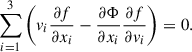
We can generalise Eq. (3) in the case where multiple lenses lie at different redshifts, creating P different lens planes. The time delay then becomes (e.g. Schneider et al. 1992)
![Mathematical equation: $$ \begin{aligned} {\Delta t_{\rm AB}} = \sum ^\mathrm{P}_{ i = 1} \frac{D_{\Delta t,i,i+1}}{c} \left[\frac{(\boldsymbol{\theta }_{\mathrm{A}, {i}}-\boldsymbol{\theta }_{\mathrm{A},{i+1}})^2}{2} - \frac{\boldsymbol{(\theta }_{\mathrm{B},{i}}-\boldsymbol{\theta }_{\mathrm{B},{i+1}})^2}{2} \right. \nonumber \\ \left. - \zeta _{i,i+1} \left(\phi _{i}(\boldsymbol{\theta }_{\rm A, {i}}) + \phi _{i}(\boldsymbol{\theta }_{\rm B, {i}})\right) \right], \end{aligned} $$](/articles/aa/full_html/2026/02/aa56411-25/aa56411-25-eq8.gif) (4)
(4)
 (5)
(5)
 (6)
(6)
By defining DΔt, eff ≡ DΔt, l, s as the time-delay distance between the main lens plane and the source plane, the time delay can be rewritten
 (7)
(7)
With the effective Fermat potential
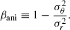
![Mathematical equation: $$ \begin{aligned} \Delta \phi ^\mathrm{eff}(\theta ) = \sum ^\mathrm{P}_{i = 1} \frac{1+z_{i}}{1+z_{\rm d}}\frac{D_{i} D_{i+1}D_{\rm ds}}{D_{\rm d} D_{\rm s} D_{i,i+1}} \left[\frac{(\theta _{i} - \theta _{i+1})^2}{2} - \zeta _{i,i+1} \psi _{i}(\theta _{i}) \right]. \end{aligned} $$](/articles/aa/full_html/2026/02/aa56411-25/aa56411-25-eq12.gif) (8)
(8)
As pointed out by Falco et al. (1985), the observables of a strong lensing system, such as the image position and the flux ratios, are invariant with respect to the mass-sheet transform (MST). This transformation of the convergence κ(θ) and the source plane coordinates β can be written as
 (9)
(9)
 (10)
(10)
This degeneracy between the mass of the lens and the size of the source is called the mass-sheet degeneracy (MSD) and implies a degeneracy between H0 and the time delay.
Although a pure mass sheet extending up to infinity in the lens plane is unphysical, the MSD is the manifestation of two physical effects: (1) the lensing effect of all the galaxies along the LOS other than the main lens. We refer to this effect as the external MSD, and it can be treated as equivalent to a mass sheet with a surface mass density κext in units of the critical density for lensing; (2) the internal mass sheet degeneracy, which results from a small mismatch between the true mass profile of the lens and its model.
The total internal and external MSD parameters defined in Eq. (9) can therefore be decomposed into two terms
 (11)
(11)
where λint is the internal MSD parameter.
The external part of the MSD can be statistically derived if κext is estimated from the mass of the galaxies along the LOS. This can be done either by counting the galaxies in a large aperture and comparing the density of the LOS to numerical simulations (see e.g. Wells et al. 2023, for detail) or with weak lensing (Tihhonova et al. 2018, 2020). The time-delay distance DΔt can then be corrected DΔt = DΔt′/(1−κext), where DΔt′ is the time-delay distance from mass modelling without accounting for κext. The detailed computation of κext is presented in Section 5.4.
Following previous TDCOSMO single-lens analyses (Wong et al. 2017; Rusu et al. 2020; Shajib et al. 2020; Wong et al. 2024), we assumed no internal MST (i.e. λint = 1). The next collaboration milestone that will hierarchically model all TDCOSMO lenses will release this parameter.
2.2. Kinematic modelling
The kinematic observable is the luminosity-weighted line-of-sight projected stellar velocity dispersion, denoted as σLOS. It is measured by targeting stellar absorption lines and quantifying their width with high-resolution spectra.
As in TDCOSMO25, we used the spherically aligned Jeans anisotropic modelling (JAM) method. This method builds on the orbital distribution f(x, v) of position and velocity of the stars in 3D motion in the galactic potential Φ. This potential is described by the steady-state collisionless Boltzmann equation (Binney & Tremaine 1987, hereafter, BT, Eqs. 4–13b)
 (12)
(12)
We then obtain a single spherical Jeans equation (BT Eqs. 4–54)
![Mathematical equation: $$ \begin{aligned} \frac{\mathrm{d} \left[\rho _*(r)\sigma ^2_{r}(r)\right]}{\mathrm{d} r} + \frac{2{\beta _{\rm ani}}(r)\rho _*(r)\sigma _{ r}^2(r)}{r} = -\rho _* \frac{\mathrm{d}\Phi (r)}{\mathrm{d} r}, \end{aligned} $$](/articles/aa/full_html/2026/02/aa56411-25/aa56411-25-eq17.gif) (13)
(13)
with ρ*(r) the stellar density distribution and βani the orbital anisotropy, defined as a function of the ratio of tangential over radial velocity dispersion components, σθ and σr
 (14)
(14)
Given σLOS, the values of σr and σθ are degenerate, leaving βani nearly unconstrained.
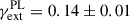
This introduces a degeneracy between σLOS and the 3D mass profile known as the mass-anisotropy degeneracy (MAD) (Binney & Mamon 1982; Merritt 1985). As demonstrated in Appendix A.2, the lens galaxy of HE 1104−1805 is a slow rotator. We hence followed TDCOSMO Collaboration (2025), and use the measurements of Cappellari et al. (2007) on slow rotating galaxies to apply the uniform prior  .
.
A solution of Eq. (13) is given by
 (15)
(15)
with M(r) the mass enclosed within the radius r and
![Mathematical equation: $$ \begin{aligned} \mathcal{J} _{ \beta }(r,s) = \exp \left[\int ^{ s}_{ r} 2{\beta _{\rm ani}} (r\prime ) \frac{\mathrm{d}r\prime }{r\prime }\right]. \end{aligned} $$](/articles/aa/full_html/2026/02/aa56411-25/aa56411-25-eq21.gif) (16)
(16)
We then get the modelled velocity dispersion along the LOS,  with (BT, Eqs. 4–60)
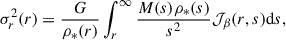
![Mathematical equation: $$ \begin{aligned} \left({\sigma ^\mathrm{LOS}}_{\rm model}\right)^2 =\frac{2}{\Sigma _*(R)} \int _{ R}^{\infty } \left[1-{\beta _{\rm ani}}(r)\frac{R^2}{r^2}\right]\frac{\rho _*(r)\sigma _{ r}^2(r)}{\sqrt{r^2-R^2}}r \mathrm{d}r, \end{aligned} $$](/articles/aa/full_html/2026/02/aa56411-25/aa56411-25-eq23.gif) (17)
(17)
with R the projected radius and Σ* the enclosed surface stellar density, which can be constrained from the luminosity profile of the lens I(R) assuming, for instance, a constant mass-to-light ratio ΥΣ*(R) = ΥI(R).
To compare this with the observed velocity dispersion along the LOS, σLOS, we weigh  with the point spread function (PSF, 𝒫) convolved light profile of the lens
 (18)
(18)
Following the methodology of TDCOSMO25, we did not account for the inclination angle of the lens galaxy during the JAM modelling. To prevent bias raised by Huang et al. (2025), we adopted the axisymmetric correction factor proposed by these authors. This factor was computed using the shape distribution from Li et al. (2018) and assuming random inclination. We then bin this factor in the same fashion as the IFU data (see Section 4.2 for more details) to obtain a correction factor for each bin, respectively: 0.992 ± 0.004, 0.977 ± 0.001, and 0.993 ± 0.004.
The final σLOS to be compared with data is then given by
 (19)
(19)
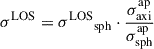
The prediction of the observed LOS velocity dispersion from any model, irrespective of the approach, can be decomposed into a cosmology-dependent ratio of angular diameter distances and a cosmology-independent part following Birrer et al. (2016, 2019)
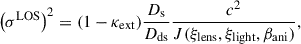 (20)
(20)
 (21)
(21)
where the dimensionless quantity J relies on the deflector model parameters (ξlens and ξlight) and βani. Moreover, J considers observational conditions and luminosity-weighting within the dispersion measurement aperture, as previously demonstrated in studies such as Binney & Mamon (1982) and Treu & Koopmans (2004).
As the angular diameter distances are sensitive to Ωm only to the second order, they are primarily sensitive to H0. Large samples of lenses and combination with probes independent from Time-delay Cosmography are required to constrain other parameters (e.g. Linder 2011; Shajib et al. 2025).
3. Time-delay measurement
3.1. Optical photometric monitoring
As one of the first discovered strongly lensed quasars, multiple attempts at measuring the time delay of HE 1104−1805 with different observation campaigns have been published in the literature. First, Wisotzki et al. (1998) published 18 spectroscopic observations with the 3.6 m ESO telescope spanning over 5 years and estimated that the time delay between images A and B, ΔtAB, should be between 109 and 292 days. Reanalysis of these data by Gil-Merino et al. (2002) and Pelt et al. (2002) showed that this sampling is insufficient for a precise delay. With a better sampling of the R-band photometry between 1997 and 2006 with the OGLE and SMARTS programs3, Poindexter et al. (2007) estimated ΔtAB = 152 ± 3 days using a Legendre-polynomial fitting technique. Later, Morgan et al. (2008) re-estimated to ΔtAB = 162.2 ± 6.1 days by jointly fitting the time delay and accretion disk size of the quasar by exploiting the microlensing signal contained in the light curves. However, the method employed depends on physical assumptions about the quasar accretion disk profile and population of microlenses that could bias the measurement.
In this work, we used three new unpublished datasets and applied the established PyCS spline-fitting method to re-estimate the time delay of HE 1104−1805 in a data-driven way without relying on any prior assumption about physical properties of the system. The first dataset is provided by the SMARTS telescope, which monitored it from 2003 to 2016 with a ∼ weekly cadence. Next, the COSMOGRAIL program (Courbin et al. 2005) observed it every ∼4 days with ECAM and C2 at the Leonhard Euler 1.2 m Swiss Telescope from 2013 to 2018 and during the 2017 season with WFI at the MPG/ESO 2.2 m Telescope every ∼2 days. These three datasets are called SMARTS, ECAM, and WFI, respectively.
For each dataset, the quasar images’ photometry was measured with the same methodology as Millon et al. (2020a) that we briefly summarise here. After bias, flat, and sky corrections, each exposure’s PSF is modelled as a Moffat profile fit combined with regularised pixel adjustments of five stars with similar luminosity as the lens in the field. The MCS deconvolution algorithm (Magain et al. 1998) is then applied to the lensed images in order to deblend the flux of an image from its counterpart, the lensing galaxy, and the arc.
Finally, a deconvolution of reference stars is carried out using the previously built PSF. Stars displaying the most photometric stability are chosen to calculate a median photometric normalisation coefficient for each exposure. This step helps to correct image-to-image systematics resulting from PSF variations across epochs. Fig. 1 shows a stack of the exposures taken with the WFI, with the stars used to compute the PSF and the normalisation of each epoch.
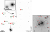 |
Fig. 1. Left panel: Stack of 280 WFI exposures of the field of view used for light curve extraction. Stars nominated PSF1 to PSF5 are used to model the PSF of each exposure, and stars designated as N1 to N5 are used to normalise the flux between each exposure. Right panel: HE 1104−1805 imaging in the filter F160W band using HST WFC3. The main lensing galaxy is denoted as G, whereas the main perturbers within 5″ of the lens are numbered from P1 to P9. |
The resulting light curves are shown on the top panel of Fig. 2. The three monitoring datasets presented are merged into a single light curve by fitting for possible magnitude and flux shifts between instruments on the overlapping parts of the light curves. The resulting combined dataset is referred to as ‘ECAM+SMARTS+WFI’.
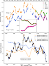 |
Fig. 2. Top panel: HE 1104−1805 R-band light curve obtained by joining three datasets: SMARTS (yellow and blue squares), ECAM (purple and green circles), and WFI (brown and pink triangles). For clarity, the light curve of B was shifted by –1.05 mag. The inset zooms on the WFI dataset span, showcasing its superior sampling to the ECAM dataset. Bottom panel: Example of a simultaneous fit of an intrinsic light curve with η = 45 days and nml = 15. The time shift obtained by this fit gives a point estimate of the system’s time delay. By repeating such measurements with randomised starting points 800 times, we obtained the time-delay measurement of this (η, nml) configuration. |
3.2. Curve shifting procedure
The time delay was computed using the method described extensively by Millon et al. (2020b), relying on free knot spline fitting implemented in the PyCS python package4 (Millon et al. 2020a). Free-knot splines are piece-wise polynomials where the mean number of days between two consecutive knots is controlled by the parameter η, which filters out variation with shorter time scales. A single free-knot spline is used to model the intrinsic variability of the quasar, which is identical in both light curves; meanwhile, an additional spline is fitted on each light curve to model the extrinsic variability caused mainly by microlensing. The number of degrees of freedom is controlled by the hyperparameter η for the intrinsic spline. For the extrinsic splines nml sets the number of knots throughout the whole curve. We fitted the intrinsic, image A and B extrinsic components, and the time delay between the light curves. A visual first guess of the time delay is used as a starting point of the fit 5. The bottom panel of Fig. 2 shows an example of such a fit, giving us a point estimate of the time delay.
We repeated the fit 800 times with starting points randomised uniformly in a range of 10 days around the first guess value, we took the median value as the time delay measurement for a given (η, nml).
To assess the uncertainty of this measurement in a data-driven way, a set of mock light curves is generated with built-in time delays uniformly drawn in an interval of ±10 days around the median value obtained previously. we used the generative noise model described by Millon et al. (2020b) to ensure that the simulated light curves have the same noise properties as the real data. The distribution of the difference between the measurement and the truth for each of the mocks gives an estimation of the systematic uncertainty (mean of the distribution) and the statistical uncertainty (standard deviation) of the time delay estimation. The final uncertainty of the time delay estimation is the sum in quadrature of these two sources of uncertainty.
The choice of values for η and nml is guided by the fact that quasars vary significantly faster than microlensing. Moreover, whether a given feature is mathematically attributed to the intrinsic or extrinsic splines depends on the flexibility balance between the splines. We therefore reproduced the same measurement for different values of these two hyperparameters. Following Millon et al. (2020b), we took η ∈ [25, 35, 45, 55] days and nml ∈ [9, 11, 13, 15] days when fitting the SMARTS, ECAM, and the merged datasets. In contrast, the microlensing in the much shorter WFI dataset is fitted with a spline having either one or two knots (nml ∈ [1, 2]) since the microlensing variability is expected to alter the light curve on time scales longer than a year.
The left panel of Fig. 3 shows the time-delay measurements obtained for each hyper-parameter configuration (η, nml) considered. The measurements obtained are consistent with each other with variable precision. We note that for a given nml, fits with η = 55 are slightly lower, which shows that the intrinsic fit is marginally too rigid. We are therefore conservative by keeping this value and should not use higher values for η. We gradually marginalised the most precise measurement with the others in order of increasing precision until the tension with the rest of the sample is lower than the threshold τ. Following the methodology of Millon et al. (2020b), we used τ = 0.5 (i.e. no individual measurement is further than 0.5σ away from the final measurement) to have a conservative uncertainty estimation without being biased by outlier measurements.
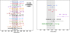 |
Fig. 3. Left panel: Measurements of the time delay for different configurations of (η, nml) with the merged ECAM+SMART+WFI dataset. Right panel: Measurement of ΔtAB for the different datasets. Since the datasets overlap, they cannot be considered fully independent. We therefore use our estimate on the joint dataset ECAM+SMARTS+WFI (green data point) as our final estimate. In both panels, the ‘combined τ = 0.5’ value was obtained by marginalising over the measurements listed above it. |
Since the three variability components are degenerate and not physically informed, the resulting splines cannot be interpreted as the true source and microlensing variations. However, a visual inspection shows that the magnitude scales of the extrinsic variations are below 0.3 mag over several years, consistent with the expected microlensing behaviour (e.g. Mortonson et al. 2005; Schneider et al. 2006; Mosquera & Kochanek 2011). We, however, note that the number of features in the extrinsic splines is higher than in most systems, which hints towards a more complex microlensing behaviour, as observed by Schechter et al. (2003) in previously published light curves, making the extrinsic fit sensitive to the hyperparameter changes.
The same experiment is carried out separately for each dataset, and the right panel of Fig. 3 shows the time delay measured in each case, the combined value, and the measurement on the merged ECAM+SMARTS+WFI dataset. The marginalisation over the three datasets would be relevant if each dataset were subject to different sources of systematic errors in the photometric measurement. However, the photometry was computed with the same method for each dataset, and no discrepancies were observed between time delays measured with ECAM and WFI data on other lens systems (e.g. Millon et al. 2020b,a). As shown by the lower panel of Fig. 2, the extrinsic variations are complex during the 2017 season. The particular case of WFI is challenging because it covers only 253 days: given the long time delay, the light curves overlap on less than 100 days. Even though distinct features are visible and well-sampled in the WFI data, the complexity of the microlensing noticed previously cannot be adequately modelled with a single season. The time delay with the WFI dataset is, thus, not robust enough for the marginalised time delay value to be trusted. Therefore, we preferred to use the ECAM+SMARTS+WFI dataset, which allowed us to use the entire period of the light curve to constrain the microlensing behaviour as well as to take advantage of the high cadence and high signal-to-noise (S/N) display of the WFI dataset.
We did not take into account a possible microlensing time delay (Tie & Kochanek 2017) because it impacts the time delay only by a day in the worst cases (Bonvin et al. 2018), which is negligible given the length of the time delay. Therefore, we use the time-delay  days, i.e. a 5.8% precision for our cosmography analysis.
4. Spatially resolved kinematics of the lens
4.1. Integral field unit spectroscopy with MUSE
A 660-second IFU observation of the system was carried out with the multi-unit spectroscopic explorer (MUSE) instrument (Bacon et al. 2010) on March 13th 2019, in wide-field mode with adaptive optics (PI: A. Agnello, program 0102.A-0600(A) and 106.215F.001). The observation wavelength ranges from 4700.03 Å to 9351.28 Å with a spectral resolution of R ∼ 2500 corresponding to an instrumental dispersion of  . The spatial resolution is 0.2″ pixel−1 and the mean seeing throughout the wavelength after the adaptive optic correction is ∼0.57″. The data reduction has been carried out as in Sluse et al. (2019), using the MUSE reduction pipeline.
This range includes the lens redshifted lines CaH [MYAMP] K lines at 3933 Å and 3968 Å along with the G-band at 4304 Å, while 5806 Å to 5965 Å wavelengths were cut out due to the notch filter. The data cube integrated across wavelength is shown in the top panel of Fig. 4. To ease spectral deblending of the quasar images from the lens galaxy, we subtracted the point source light at each wavelength of the data cube. To do so, at each wavelength, the point sources and lens galaxy light are fitted simultaneously with a Moffat and Sérsic profile with relative positions fixed to the ones measured on the HST data. For each wavelength frame, the Moffat part of the fit is then subtracted from the data to obtain the data cube displayed in the inset of Fig. 4.
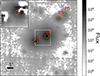 |
Fig. 4. MUSE data cube summed over all wavelengths. The inset displays the point-source subtracted cube, revealing the lens galaxy light. The apertures used to extract individual spectra of the quasar images, lens centre, and perturbers shown in Fig. B.1 are represented by orange circles. |
The spectrum of the centre of the lens galaxy obtained from this subtracted cube is shown in Fig. B.1 and displays observation with an S/N of 30 Å−1, which is used to measure σLOS. We also retrieved new high-quality quasar spectra thanks to a small aperture integration on images A and B, and the spectra of some perturbers annotated on Fig. 1 (See Appendix B.1). Finally, we extracted the spectra of the two brightest perturbers (P5 and P6) with a sufficiently high S/N (∼ 11 Å−1 and ∼ 7 Å−1 respectively) to measure their redshifts.
4.2. Stellar template fitting
As shown by the left panel of Fig. 5, we masked the pixels from the lens light cube further than 1.8″ from the centre of the galaxy, as well as an area of 0.8″ around the position of images A and B. In order to maximise the number of constraints on the radial velocity profile, the frame is then divided into three concentric rings of 0.53″ width with S/N from 14 Å−1 to 30 Å−1. The integrated spectra of each bin are then fitted using the penalised pixel fitting (pPXF) method6 (Cappellari 2017, 2023). This method models the galaxy spectrum with a weighted linear combination of stellar spectra, broadened by a convolution with the galaxy line-of-sight velocity distribution. Additive Legendre polynomials are included in the model to improve the robustness to template mismatch and dust reddening. Furthermore, a multiplicative polynomial accounts for spectral flux calibration mismatches between data and templates. Any contaminating signal from residuals of the quasar images blended with the galaxy is accounted for by including a scaled quasar spectrum presented in Fig. B.1.
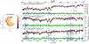 |
Fig. 5. Velocity dispersion point-estimate in the three radial bins of HE 1104−1805’s lens galaxy. Left panel: Mean of the MUSE data cube after PSF subtraction and masking with overlaid bin numbers and contours. Right panel: Example of a pPXF fit of the integrated spectra of each bin, where data masked for the fit are marked in grey. |
As shown in Fig. B.1, the most constraining features of the lens galaxy spectrum for the σLOS measurement are the CaH, CaK, and G-band absorption lines identified respectively at 6800 Å, 6828 Å and 7395 Å in the observed frame. To focus the fit on these lines and avoid regions of the spectrum that could be dominated by the C IV and C III emission of the quasars, we restricted the wavelength range to [6220, 7780] Å (in the rest-frame [3600, 4400] Å).
Following Knabel et al. (2025), we used three stellar template libraries: Indo-US (Valdes et al. 2004), MILES (Sánchez-Blázquez et al. 2006; Falcón-Barroso et al. 2011), and X-shooter spectral library (Verro et al. 2022), cleaned from incomplete or low-quality spectra and convolved them down to the same FWHM as the observation’s Line Spread Function in the galaxy’s rest frame, estimated at 1.46 Å with the empirical relation given by Bacon et al. (2023).
An exploratory set of fits allowed us to determine that an additive polynomial of degree 6 combined with a multiplicative polynomial of degree 0 yields the most robust measurements across the different template libraries.
An example of the σLOS estimate in each bin given by a fit with this fiducial setup is shown in Fig. 5.
We then combined the fits from different template libraries using the bayesian information criterion (BIC, Schwarz 1978). It is defined as:
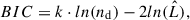 (22)
(22)
where  is the maximised value of the likelihood function of the model M, i.e.
  , where
  are the parameter values that maximise the likelihood function, nd is the number of data points (i.e. the number of unmasked spectral pixels), k is the number of parameters in the model.
The central value and statistical uncertainties are given by the BIC-weighted mean of the measurements obtained with the different libraries, while the systematic uncertainty is computed as the weighted-mean difference between the central value and each library measurement.
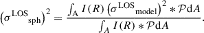
To test the robustness of the measurement against potential contamination of the CaK and G-band by sky emission lines, we repeated the measurement while masking the first ([3954;4000] Å) or the latter ([4275;4325] Å). We obtained measurements in excellent agreement with the original one and therefore use this one for the cosmographic analysis.
The final measurement, along with the corresponding covariance matrix, is shown in Table 1.
σLOS measurements and covariance matrix of each bin.
5. Line-of-sight analysis
5.1. Wide-field imaging
The HE 1104−1805 field was targeted by a multi-band imaging campaign to assess the contribution of line-of-sight structures to the lensing signal. The data acquired included u-band with a total exposure time of texp = 20 706 s with Megacam on the Canada France Hawaii Telescope (Program ID: 14AT01; PI Suyu); Subaru SuprimeCam imaging in the g (texp = 600 s), r (texp = 4800 s), and i (texp = 600 s) bands (Program ID: o14220; PI Fassnacht, the latter is shown in Fig. 6); and Subaru MOIRCS near-infrared imaging in the J (texp = 3600 s), H (texp = 5760 s), and Ks (texp = 2940 s) bands (Program ID: o15202; PI Fassnacht). For the current analysis of the line-of-sight, we only considered the SuprimeCam imaging.
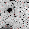 |
Fig. 6. Wide-field imaging of HE 1104−1805 in the i-band. Red circles denote regions within 8″, 45″ and 120″ of the centre of the lens. |
The SuprimeCam data were reduced in a two-phase process. The initial steps utilised the SDFRED reduction package to do the overscan and bias correction, flat-field correction, distortion and atmospheric distortion corrections, and masking of some bad regions. The second phase used custom Python-based scripts to mask bad pixels and to combine the individual exposures.
The SuprimeCam imager provides a field of view of approximately 30′ on a side, which is substantially larger than what is needed for the analysis presented in Sect. 5.4. We therefore used only a 4′ × 4′ section centred on the lens system to generate the galaxy catalogues. The catalogues were produced by running SExtractor (Bertin & Arnouts 1996) in dual-image mode, using the deep r-band data as the detection image and the i-band image as the measurement image. The photometric zeropoints were determined by comparing the instrumental magnitudes of stars in the field to the magnitudes measured by SDSS for those stars.
5.2. Perturbers and groups explicitly included in the lens model
As shown in Fig. 1, we identified nine perturbers within 5″ of the lens in the HST imaging. Our initial step, hence, involved identifying the perturbers that we need to explicitly include to the lens model.
The ‘flexion shift’ was introduced by McCully et al. (2017) to determine which line-of-sight galaxies should be explicitly included in the lens modelling and which ones should be implicitly accounted for through the computation of κext.
The specific influence of line-of-sight objects depends on whether the dominant-lens approximation holds, indicating that the critical density of these objects is much smaller than that of the primary deflector (Fleury et al. 2021).
The difference in lens image position induced by a given nearby galaxy is given by:
 (23)
(23)
with θE, lens and θE, pert as the Einstein radii of the lens and perturber, and θ as the angular separation of the lens and perturber. The function f(β) equals 1 if the perturber is between the lens and the observer, while f(β) = (1−β)2 if the perturber is behind the main lens. β is the pre-factor of the lens deflection in the multi-plane lens equation: β = (DdpDs)/(DpDds). McCully et al. (2017) found that perturbers with Δ3x ≤ 10−4 are accurately accounted for with a global external convergence term, whereas perturbers with a higher flexion shift should be individually modelled with a multi-plane treatment.
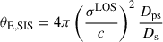
We used the M* − σLOS relation obtained Zahid et al. (2016) on galaxies up to redshift 0.7 to estimate the mass-to-light ratio, M/L, of the P5 perturber using its velocity dispersion σLOSP5 measured with the MUSE data (see Appendix B.2 for more details). The flux determined with a circular aperture around P5 in the F160W band converted into luminosity using a fiducial cosmology with H0 = 70 km s−1Mpc−1 and Ωm = 0.3. By applying the same M/L ratio to the other perturbers, we estimated their mass and σLOS. Given the uncertainty of the  measurement, the uncertainty on the fiducial cosmological parameters and the fact that some perturbers are assumed to be further than the range studied by Zahid et al. (2016), can be neglected. By approximating the perturbers’ mass distributions with an SIS, we computed their Einstein radius, θE, SIS, with :
 (24)
(24)
with Dps and Ds the angular diameter between the source and perturber, and between the observer and the source, respectively.
We assumed that the perturbers without a redshift measurement lie between the closest perturber, P5 and the source. We therefore repeated the computation with redshifts uniformly drawn between z5 and zs, and took the mean, the 16th, and 84th percentile (1 − σ in a Gaussian distribution) of the resulting distribution as the final estimate.
We could then estimate the flexion shift caused by each perturber using Eq. (23). The results presented in Table 2 show that even when marginalising on their redshift, the flexion-shifts of these perturbers are all potentially larger than 10−4. They can therefore significantly influence the image’s position and should be included in the mass model.
In addition, the subtraction of the PSF, lens, and source light with a preliminary SIE model revealed the presence of a luminous component ∼0.6″ from image B. Without a counter-image indicating that this feature belongs in the source, we treated this component as a perturber, hereafter P9. Because of its faintness, the spectra of P9 could not be extracted from the MUSE data cube, and its mass could not be estimated with the same technique employed for all other perturbers.
5.3. Identification of galaxy groups in the vicinity of the lens
Our search for galaxy groups along the line-of-sight relies on a catalogue of spectroscopic redshifts of field-of-view galaxies. To compile that catalogue, we have obtained multi-object spectroscopy of galaxies up to ∼2 arcmin using the FORS2 instrument mounted on the Antu VLT telescope (PID: 092.0515, PI: D. Sluse), and using GMOS at the Gemini-South Telescope (PID: GS-2013B-Q-28; PI: T. Treu). The observational setup, data reduction, and target selection strategy are similar to the one described in Sluse et al. (2017). Individual spectra typically cover the range 4500–9200 Å for FORS2 data and 4400–8200 Å for GMOS. Within a 30″ radius around the lens, we also extracted spectra of the sources present in the MUSE data used for kinematics (Sect. 4.2). We used 1D cross-correlation methods to measure redshifts: the xcsao task implemented in IRAF was used for the FORS data, and MARZ (Hinton et al. 2016) was used for the other data sets. This yields an ensemble of 131 reliable unique redshifts (96 with FORS2, 18 with GMOS, 17 with MUSE) distributed typically in the range z ∈ [0.04, 0.8]. We complemented the catalogue with redshift measurements from Momcheva et al. (2015) who targeted galaxies as faint as I ∼ 21 mag within a radius of 15 arcmin of HE 1104−1805. This sample adds 387 unique redshifts to the catalogue, out of which 47 are within a radius of 6 arcmin of the lens, i.e. the region where we expect groups to have first-order contribution to the main lens gravitational potential.
The identification of galaxy groups is done using the algorithm described in Sluse et al. (2017), Sluse et al. (2019), and Buckley-Geer et al. (2020), and we refer the reader to these publications for details. This algorithm is based on the group-finding algorithms of Wilman et al. (2005) and Ammons et al. (2014). For this measurement, we have computed the group centroid from the luminosity-weighted positions of the group members. The groups likely to perturb the modelling of the main lens are summarised in Table 2. Groups 4, 5, and 6 highlight the group finder’s sensitivity to initial conditions and interlopers, with some galaxies appearing in multiple groups. We therefore included them separately in the lens models (see Sect. 6). In Fig. D.1, we show, for each identified group, the right ascension and declination of the accepted and rejected member galaxies as well as the distances and velocities relative to the final group centroid.
Galaxies and groups of galaxies identified as potential perturbers.
5.4. External convergence (κext) measurement
Similar to the previous time-delay cosmography studies (e.g. Rusu et al. 2017; Birrer & Amara 2018; Rusu et al. 2020), we used the number count technique to determine κext. This quantity determines the contribution of objects not included in the lens modelling. Number counts involve measuring the galaxy number density near the lens as a summary statistic and comparing it to reference fields. This comparison helps determine whether the LOS is over- or under-dense compared to the average background (e.g. Fassnacht et al. 2011; Greene et al. 2013; Wells et al. 2023).
It can be summarised in four main steps:
-
Lines of sight (typically several arcminutes wide squares) are drawn from a large comparison field and compared to the LOS of the lens. Modern survey datasets covering hundreds to thousands of square degrees ensure a sufficiently large comparison field to avoid sampling bias. The photometric catalogues of the fields are cleared from objects more distant than the lensed source and fainter than the used magnitude cut on the i < 24 (e.g. Fassnacht et al. 2011). This cut is designed to consider only objects with reliable photometry.
-
The weight value of a given LOS Wi is then computed as the ratio of the weighted number counts for galaxies in the lens field to the same statistic in the reference field.
 (25)
(25)where j indexes the galaxies in a given LOS and w is the weight of a galaxy. Different types of weights can be considered (e.g. Greene et al. 2013; Rusu et al. 2017; Wells et al. 2023) such as the galaxy’s distance to the center (1/rj), its potential (mj/rj), its redshift (zj(zs − zj)) or simply be the same for each galaxy (wj = 1). The weight value obtained, therefore, acts as a tracer of the external convergence of the lens LOS.
-
Similar weight values are computed in simulated fields with known κext (Hilbert et al. 2009). Previous works (e.g. Rusu et al. 2017; Wells et al. 2023), have shown that using the Millennium Simulation yields a reliable estimate of κext because it provides catalogues of galaxies for several values of the external convergence at sufficient points to represent the Universe accurately. Since the weight value relies on ratios, many dependencies on the simulation’s underlying cosmological parameters are expected to cancel out.
-
The posterior probability of κext can hence be computed as follows
 (26)
(26)Here, p(W|d) represents the probability distribution of the weighting scheme W given the data, and psim(κext|W) denotes the probability distribution of κext in the simulated dataset, conditioned on a specific value of the weight W. Greene et al. (2013) showed that the combination of multiple evaluations relying on different weights (while adequately taking into account covariances between estimates) significantly improves the precision and robustness of the measurement.
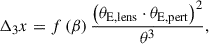
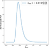 |
Fig. 8. κext measurement showing that the line-of-sight of HE 1104−1805 is along a slightly underdense region of the Universe. Therefore, the fact that multiple perturbers are near the main lens is coincidental and the approximation κext ≈ κs holds. |
As detailed previously, the treatment of perturbers within 5″ from the lens is part of the explicit lens model. We, therefore, masked this region from the number counting and removed the galaxies forming the perturber groups presented in Table 2, as in Wells et al. (2023), we limited the field to 120″ around the lens. The weights used are the number counts w1 and the inverse distance w1/r of objects. Their computation is displayed in Fig. 7 and Fig. 8 displays the final measurement 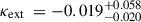 . Our procedure, in fact, determines κs, the convergence up to the source which we used as a proxy for κext. The external convergence is technically computed using the observer-deflector and deflector-source convergences (κd and κds) through κext = (1−κd)/(1−κs) ⋅ (1−κds). However, Tang et al. (2025) showed that ignoring this correction affects the H0 measurement only when the LOS up to the deflector is significantly over- or under-dense, which is not the case here. At the population level, the expected bias on H0 due to this approximation is about 0.1%, which is negligible compared to the present 4.6% precision of TDCOSMO25.
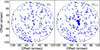 |
Fig. 7. Position and weight (size of the dot) of galaxies between us and the source. Black circles indicate the 45″ and 120″ apertures. Blue dots correspond to objects with i-magnitudes less than 24. |
Therefore, this measurement is used for the rest of the cosmographic analysis, without further correction, in compliance with the perturber inclusion strategy.
6. Lens modelling
6.1. HST imaging
In the context of H0LiCOW (Suyu et al. 2017), Program 12889 (P.I: S.H. Suyu) took 12 exposures of 36 seconds along with 24 exposures of 599 seconds of HE 1104−1805 with wide-field camera 3 (WFC3) in the F160W7 band. A 4-point dither pattern with parallelogram shapes having half-pixel shifts was applied in order to reach a resolution of 0.08″ per pixel. The imaging displayed in the left panel of Fig. 1 showcases the main challenges for modelling this system. First, the point source images are particularly bright with the PSF wings of both images aligned with the centre of the galaxy. Accurate modelling of the PSF’s wings is, therefore, crucial to model the light of the lens. Secondly, the quasar host’s light is very dim and distinguishable only after proper subtraction of the lens light (see Fig. C.2). This makes the lens light fitting a primordial and sensitive step to properly reconstruct the shape of the arc, a key constraint to mass modelling. Thirdly, the system’s environment is particularly crowded with eight luminous galaxies within 15″ of the main lens. The system is also characterised by a large and asymmetric separation of images A and B positions from the lens centre of 1.17″ and 2.05″, respectively.
6.2. Setup and workflow
6.2.1. Main deflector mass and light model
Following the methodology of the most recent TDCOSMO lens models (e.g. Shajib et al. 2020, 2022), we modelled the lens galaxy with two families of models: power law and a composite alternatively.
In the first case, the mass is parametrised as a power-law elliptical mass distribution (PEMD) for which the convergence at the position (θ1,θ2) in the frame aligned with the major and minor axis of the deflector is given by
 (27)
(27)
where θE is the Einstein radius, γPL the slope of the profile, and qm its axis ratio. This convergence map is then rotated by the position angle ϕm to belong to the on-sky coordinate frame.
The lens light is modelled by a superposition of two Sérsic profile which gives the light intensity at the position (θ1,θ2) following
![Mathematical equation: $$ \begin{aligned} I_{\rm {Sersic}}\left(\theta _1,\theta _2\right) = I_{\rm eff}\exp \left\{ -b_{ n}\left[\left(\frac{\sqrt{\theta _1^2+\theta _2^2/q^2}}{\theta _{\rm eff}}\right)^{ 1/n}-1\right]\right\} \end{aligned} $$](/articles/aa/full_html/2026/02/aa56411-25/aa56411-25-eq89.gif) (28)
(28)
with θeff the effective radius (i.e. the product average of semi-major and semi-minor axis), also defined as the half-light radius, thanks to the normalising factor bn, Ieff the intensity at θeff. q is its axis ratio, and n the Sérsic index.
The positions of the two Sersic profiles are tied together throughout the fit, and the position of the mass component’s centre is fixed on the light component.
The chameleon profile can be parametrised as the difference between two non-singular isothermal ellipsoid (NIE) profiles (e.g. Suyu et al. 2014)
![Mathematical equation: $$ \begin{aligned} \kappa _{\rm Chm}(\theta _1, \theta _2) = \frac{\kappa _{0,\mathrm{Chm}}}{(1+q)} \left[ \frac{1}{\sqrt{\theta _1^2+\theta _2^2/q^2 + 4w_{\rm c}^2/(1+q)^2}} \right. \nonumber \\ \left. -\frac{1}{\sqrt{\theta _1^2+\theta _2^2/q^2 + 4w_{ t}^2/(1+q)^2}} \right] \end{aligned} $$](/articles/aa/full_html/2026/02/aa56411-25/aa56411-25-eq90.gif) (29)
(29)
where q is the axis ratio and wc and wt are sizes of the cores of the two NIE with wt >wc.
For the composite model, the baryonic mass is described by a double chameleon profile (i.e. two superposed chameleon profiles presented in Eq. 29).
The dark matter halo is modelled with an elliptical Navarro-Frenk-White (NFW) profile, whose volumic density is given by
 (30)
(30)
where ρ0 is a normalisation and Rs is the scale radius.
Following the measurement of Gavazzi et al. (2007) on galaxies that have a similar σLOS as the one measured in this system, we expect the NFW’s scale radius to be within Rs = 58 ± 8 kpc. To prevent any prior bias, we took this value as a starting point within a wide uniform prior Rs ∼ 𝒰(25 100) kpc.
We used a double chameleon profile to model the light, and the fitted parameters are fixed to the parameters of the baryonic mass model.
To avoid the lens light modelling from being biased by background light while still predicting accurate flux at the position of the arc, we masked pixels further than 4.3″ from the lens. We adjusted the mask locally to mask the light of all the perturbers and masked the lens’s central pixels because the light is not fitted perfectly in this region. Masking the few pixels close to the centre of the lens prevents the model from predicting source flux at this position, which can possibly bias the inferred mass profile.
6.2.2. Source light model
The visible source light is smooth, and we modelled it with a single elliptical Sérsic profile in both families of models. Contrary to previous TDCOSMO studies, no further structure is detected in the lensed arc. Thus, it is not required to add shapelets to describe extra complexity.
6.2.3. Perturbers’ model
To include the perturbers in the mass model, we added an SIS component to the mass model for each perturber. Even though we did not fit their light in the final model, a preliminary Sérsic fit gives us their position. Since P5 and P6 have different redshifts than the lens, we used the multi-lens-plane formalism introduced in Eqs. (4) and (8). For the other perturbers considered, we assumed that they lie in the same plane as the lens. We considered the perturbers P2, P5, and P6 as they have the highest flexion shifts, and P9 because of its proximity to image B. Furthermore, the perturber groups listed in Table 2 are parametrised with NFW profiles. We estimated their scale radii using their virial mass (based on measured R200 and vdisp) and estimation of the NFW concentration parameter, R200/RS from Duffy et al. (2008). The groups 4, 5, and 6 are alternatively included in the model.
6.2.4. PSF modelling
To complete the light model, each component is convolved by the PSF. As a first guess of the PSF, five stars of the field were stacked together using the PSFr software (Birrer et al. 2022).
Since the spectrum of the stars in the field used for the PSF initial guess does not match the quasar one, we finalised the PSF model with four successive repetitions of the following sequence with the Lenstronomy software8 (Birrer & Amara 2018):
-
mass and light model parameter optimisation using Lenstronomy’s built-in particle swarm optimiser routine (e.g. Eberhart & Kennedy 1995; Birrer & Amara 2018)
-
iterative reconstruction of the PSF on lens and source subtracted residuals. We also adjusted the PSF noise map in a radius of 0.5″ around its centre to adapt the constraining power of these pixels.
6.2.5. Posterior sampling and combination of different models
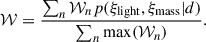
After obtaining a satisfactory PSF, shown in Fig. C.1, we used Lenstronomy’s built-in MCMC routine relying on EMCEE (Foreman-Mackey et al. 2013) to sample the light and mass parameters (ξlight and ξmass) posterior by maximizing the likelihood expressed as
 (31)
(31)
where ℒ(d|ξlight, ξmass) is the likelihood of the parameters given the data and p(ξlight, ξmass) is the prior on the parameters. During this step, the data used to constrain the posterior are the unmasked pixels of the HST observation 𝒟Img and the time delay, ΔtAB. The likelihood maximised by the sampling is therefore computed with
 (32)
(32)
which is, up to an additive constant,
![Mathematical equation: $$ \begin{aligned} = \log \left[-\frac{1}{2}\sum _{ i}^{N_{\rm pix}} \frac{(\mathcal{D} _{\rm Img, i}- M_{\rm Img, \textit{i}})^2}{\sigma _{ i}^2}\right] + \log \left[-\frac{1}{2}\frac{({\Delta t_{\rm AB}} - M_{\Delta t_{\rm AB}})^2}{\sigma _{\Delta t_{\rm AB}}}\right], \end{aligned} $$](/articles/aa/full_html/2026/02/aa56411-25/aa56411-25-eq94.gif) (33)
(33)
where MImg and MΔtAB are the model-predicted image and time delay of the system; σi is the pixel’s noise, and σΔtAB the uncertainty on the time delay. We used ten times as many walkers as there are parameters in the model, and we used the last 1000 out of 20 000 iterations to construct the posterior of a given modelling setup. The best reconstructions of the HST imaging with power-law and composite models shown in Fig. 9 demonstrate that all relevant features in the light are correctly predicted. The convergence profile obtained by each model family in every perturber-inclusion scenario is displayed in Fig. 10. We notice that, with both model families, the convergence of the perturbers P5, P6, and G1 varies substantially between the different scenarios. This can be attributed to the fact that these components are aligned in the same direction relative to the main lens, resulting in a degenerate effect on the system. Conversely, the convergence of the perturbers P2, P9, and groups G2, G3 are more stable as they are more azimuthally spread. We also note that in every scenario, the composite model is cuspier than the power-law one.
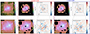 |
Fig. 9. Reconstructed image of HE 1104−1805 using the best power-law and composite models. From left to right: The imaging data, reconstructed image, and normalised residuals are displayed for the power law model (PEMD + Shear + perturbers 2, 5, 6, 9 + groups 1, 2, 3, and 4) and composite models (NFW + Double chameleon + Shear + perturbers 2, 5, 6, 9 + groups 1, 2, 3, and 4). |
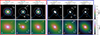 |
Fig. 10. HE 1104−1805 modelled convergence κ with the two families of models and different perturbers and groups inclusion strategies. The top row shows a wide-field including all groups and the bottom row zooms in on the region closer to the main lens; white lines indicate the area enclosing 25, 50, and 75% of the total mass. |
The BIC values computed with the maximum likelihood of each model are presented in Table 3. The variance of the BIC is σΔBIC = 73 within the power-law models and σΔBIC = 48 within the composite models.
Summary of lens modelling scenarios and their relative weight within each family.
Similarly to Birrer et al. (2019) and Shajib et al. (2022), we determined the weight of each posterior distribution following
 (34)
(34)
where f(x) is the evidence ratio function given by
 (35)
(35)
with BICmin the BIC of the reference model with the minimum BIC value.
To create a single posterior out of N multiple models, we summed all the posteriors using their normalised weights
 (36)
(36)
This procedure is done separately for the composite and power law models, and we compare the results in Fig. 11. For both models, the Einstein radius, the slope, and the time-delay distance are robust to the different perturber configurations, whereas the external shear shows multi-modality because the G6 group centre is azimuthally significantly different from groups G4 and G5 (see Fig. 10). A blind comparison of the two modelling families allowed us to see that a 2.1-σ disparity between the two families on γ induces a 1.3-σ difference in the Fermat potential and 1-σ for the time-delay distance between the two families. The external shear we inferred for HE 1104−1805 is higher than in other TDCOSMO lenses. As shown by Etherington et al. (2023), model-predicted γext in power-law + shear configurations is often overestimated even in perturber-free systems because it is degenerate with potential azimuthal structures, which have a negligible impact on H0 at the population level (Van de Vyvere et al. 2022). In Section 5.2, we considered only nine perturbers, out of which five are explicitly modelled, but many more are visible in the right panel of Fig.1. These perturbers are expected to induce external shear on the main lens and induce a large γext. More marginally, the positions of the centre of mass of the groups of pertubers, G1-G6, are poorly constrained and might also inflate the value of γext.
 |
Fig. 11. BIC weighted comparison of the power-law and composite models. For each family, we marginalised over the three posteriors given by the three perturber inclusion scenarios, which results in the multi-modality of some of the parameters such as γ. We obtained |
7. Cosmographic inference
We combined the mass and light posteriors obtained with the lensing and time delay constraints with the resolved kinematics measured in Section 4.2 to measure Dd, DΔt, and H0.
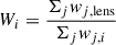
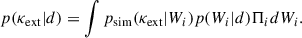
Following the methodology of Shajib et al. (2023), we importance sampled the posterior distribution of the lens model obtained with Eq. (36), ξlight, ξmass together with the cosmological distances Dd and DΔt given the three radial bins of the velocity dispersion σLOS and the external convergence κext measured
 (37)
(37)
with p(κext) the prior on κext obtained in Section 5.4.
The likelihood of the modelled 3-bin velocity dispersion is computed with the following
![Mathematical equation: $$ \begin{aligned}&\mathcal{L} ({\sigma ^\mathrm{LOS}} \vert {\sigma ^\mathrm{LOS}}_{\rm modelled} ) \nonumber \\&\propto \exp \left[ -\frac{1}{2}({\sigma ^\mathrm{LOS}}-{\sigma ^\mathrm{LOS}}_{\rm modelled})^\mathrm{T} \ \mathcal{C} ^{-1} \ ({\sigma ^\mathrm{LOS}}-{\sigma ^\mathrm{LOS}}_{\rm modelled})\right], \end{aligned} $$](/articles/aa/full_html/2026/02/aa56411-25/aa56411-25-eq103.gif) (38)
(38)
where  is the 3-bins velocity-dispersion computed with the JamPy package9 (Cappellari 2008, 2020) through Eqs. (17) and (19). 𝒞 is the covariance matrix between σLOS measured in each bin determined in Section 4.2. In practice, the software uses multi-gaussian-expansions (Emsellem et al. 1994; Cappellari 2002, MGE) fits of the mass and light profiles to be able to deproject these surface densities into 3D ones in a straightforward way (Monnet et al. 1992). The light MGE fit is based on the lens light profile corresponding to the ξlight with maximum likelihood. The PSF is modelled as a Moffat with β = 1.96 and FWHM = 0.54″ based on the mean value of these parameters along the wavelength range used for the σLOS measurement (i.e. [6000-9000] Å) that is shown in the bottom panel of Fig. 4.
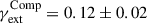
As explained in Section 2.2, we adopted a uniform prior 𝒰(−0.12, 0.13) on βani. The resulting kinematic fit for each modelling family is shown on the left panel of Fig. 12 while the associated posterior distribution of Dd and DΔt is shown in the right panel. The kinematic modelling performed without allowing for the internal mass-sheet shows that the steepness of the composite model fails to correctly fit the observed velocity dispersion profile, especially in the innermost bin, where the best fit predicts 301 km s−1, i.e 1.6 σ away from the observed value. This results in a 2.1 σ tension between the inferred Dd. The likelihood-weighted combination assigns 95 % of the final posterior to the power-law model, effectively discarding the composite model measurement.
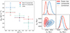 |
Fig. 12. Left panel: Kinematic fit using power-law and composite models. Red and blue central dots show the best-fit values, while error bars are the 16th and 84th percentiles of 100 predicted velocity dispersions. Right panel: Posterior of Dd and DΔt using kinematics based on the power-law and composite mass models. Using likelihood weighting we measured |
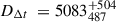
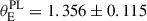
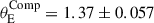
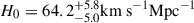
Using the posterior distribution of Dd and DΔt we then inferred H0 in a flat-ΛCDM cosmology with the purposedly conservative uniform priors 𝒰(0, 150) km s−1Mpc−1 on H0 and 𝒰(0.05, 0.5) on Ωm. The resulting posterior distributions obtained for both models and the combination are displayed in Fig. 13. As with every TDCOSMO H0 measurement, the entirety of the analysis was performed blindly to avoid confirmation bias. The final value was revealed on July 8th of 2025,  km s−1Mpc−1, i.e. an 8.5% precision from a single doubly imaged lens.
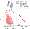 |
Fig. 13. H0 measurement with HE 1104−1805 using the joint constraint of DΔt and Dd measured with the power-law, composite models, and both models combined. Our final measurement using the likelihood weighted combination of both models is |
8. Discussion and conclusion
Table 4 summarises all the cosmography-related measurements achieved for HE 1104−1805.
Summary of all the relevant HE 1104−1805 measurements.
8.1. Time-delay
The measurement of the time delay is marginally higher than previous estimates (e.g. Poindexter et al. 2007; Morgan et al. 2008, measured ΔtAB = 162 ± 6.1 days). It relies on the longest and best-sampled light curve of that system, with the two most recent (ECAM and WFI) datasets having at least twice the cadence as the previous SMARTS dataset. It was estimated with a data-driven algorithm whose accuracy was assessed on multiple simulated and observed light curves, which is crucial, as we saw that the extrinsic variability is particularly challenging to model in this system. We therefore have the most robust estimate for this object.
8.2. Resolved kinematics
The main limitation of the resolved velocity dispersion measurement comes from the proximity and brightness of image A to the lens galaxy. Nevertheless, by subtracting the quasar images, we were able to extract spectra from three concentric bins with S/N > 14 Å−1. Using state-of-the-art methodology to constrain the effect of stellar template fitting hyperparameters (polynomial degrees and stellar template libraries), we provided the velocity dispersion measurement in each bin. We ensured the robustness of these measurements against different spectral and spatial masks and proved that the lens is a slow rotator (see Appendix A.2). The latter justifies the use of spherically aligned JAM for the kinematic modelling.
8.3. Image and kinematic modelling
The image reconstruction was performed with the two main parameterisation families: power-law and composite. Three configurations of nearby perturbers were accounted for individually, with the addition of SIS and NFW components, and the resulting measurements were marginalised upon these configurations.
The main difference between the two models resides in the slope of the radial mass profile γ. Such a difference was already observed in modelling the quadruply lensed quasar WGD 2038−4008 (Shajib et al. 2022), where the system’s compactness only allowed to probe the inner regions of the mass profile. In the present case, the resolved velocity dispersion heavily favours the power-law model over the composite for this system. This may be because HE 1104−1805’s configuration offers too few constraints for a composite model, thus leading to potential biases or simply that the power law model is a better description over the range probed. The discrepancy between the external convergence, κext, and the external shear, γext, inferred independently might be counter-intuitive in light of simulations’ properties (e.g. Tang et al. 2025). However, in this work γext is primarily encompassing the effect of perturbers within 5″ of the main deflector, whereas κext is inferred from galaxies up to 120″ away, excluding the ones within 5″. As discussed in Section 6.2.5, the large value of γext may arise from genuine external shear or simply be inflated by inherent lens-modelling degeneracies. We could not disentangle the contribution of each effect with the available data, nor rule out unmodelled convergence. However, since the brightest perturbers we considered are already low-mass (see upper part of Table 2), any additional convergence from fainter perturbers should be small.
8.4. Implications for time delay cosmography
This work shows that the high precision of the time-delay measurement and the use of resolved kinematics allowed us to reach a precision of 8.5% on H0 with a double lens quasar, which is comparable to previous TDCOSMO single lens measurements ranging from 4% to 28% (Millon et al. 2020c; Wong et al. 2024). The main limitation of this work is the fact that we fixed the internal mass-sheet degeneracy parameter, λint = 1. This parameter will be constrained during the next joint hierarchical modelling of the TDCOSMO lens sample. The H0 value and precision of this system are therefore bound to change as H0 → H0λint, (δH0 / H0)2 → (δH0 / H0)2 + δλint2.
Overall, this work is a stepping stone towards building a sample of double-lens quasar-based H0 measurement, which is vital to investigate potential biases of the TDCOSMO method and to accelerate progress towards a 1% measurement of H0.
Acknowledgments
E.P. is supported by JSPS KAKENHI Grant Number JP24H00221. F.C. is supported by the Swiss National Science Foundation (SNSF) and by the European Research Council (ERC) under the European Union’s Horizon 2020 research and innovation programme (COSMICLENS: grant agreement No 787886). C.D.F. acknowledges support for this work from the National Science Foundation under Grant No. AST-2407278. A.G. acknowledges support by the SNSF (Swiss National Science Foundation) through a mobility grant P500PT_211034. M.M. acknowledges support by the SNSF (Swiss National Science Foundation) through mobility grant P500PT_203114 and return CH grant P5R5PT_225598. D.S. acknowledges the support of the Fonds de la Recherche Scientifique-FNRS, Belgium, under grant No. 4.4503.1. S.B. acknowledges support by the Department of Physics and Astronomy, Stony Brook University. C.L. acknowledges funding from the European Union’s Horizon Europe research and innovation programme under the Marie Sklodovska-Curie grant agreement No. 101105725. A.J.S. received support from NASA through STScI grants HST-GO-16773 and JWST-GO-2974. S.H.S. thanks the Max Planck Society for support through the Max Planck Fellowship. This work is supported in part by the Deutsche Forschungsgemeinschaft (DFG, German Research Foundation) under Germany’s Excellence Strategy – EXC-2094 – 390783311. T.T. acknowledges support by NSF through grants NSF-AST-1906976, NSF-AST-1836016 and NSF-AST-2407277, and from the Moore Foundation through grant 8548. K.C.W. acknowledges support by JSPS KAKENHI Grant Numbers JP24K07089, JP24H00221. V.M. acknowledges support from ANID FONDECYT Regular grant number 1231418, Centro de Astrofísica de Valparaíso CIDI 21, and ANID, Millennium Science Initiative, AIM23-0001. This work used observations collected at the European Southern Observatory under ESO programmes 092.0515(B) and 0102.A-0600(A). This work used Python packages Numpy (Harris et al. 2020), Astropy (Astropy Collaboration 2022), and Scipy (Virtanen et al. 2020).
References
- Abdul Karim, M., Aguilar, J., Ahlen, S., et al. 2025, Phys. Rev. D, 112, 083515 [Google Scholar]
- Ammons, S. M., Wong, K. C., Zabludoff, A. I., & Keeton, C. R. 2014, ApJ, 781, 2 [Google Scholar]
- Astropy Collaboration (Price-Whelan, A. M., et al.) 2022, ApJ, 935, 167 [NASA ADS] [CrossRef] [Google Scholar]
- Bacon, R., Accardo, M., Adjali, L., et al. 2010, SPIE Conf. Ser., 7735, 8 [Google Scholar]
- Bacon, R., Brinchmann, J., Conseil, S., et al. 2023, A&A, 670, A4 [NASA ADS] [CrossRef] [EDP Sciences] [Google Scholar]
- Bertin, E., & Arnouts, S. 1996, A&AS, 117, 393 [NASA ADS] [CrossRef] [EDP Sciences] [Google Scholar]
- Binney, J., & Mamon, G. A. 1982, MNRAS, 200, 361 [Google Scholar]
- Binney, J., & Tremaine, S. 1987, Galactic dynamics [Google Scholar]
- Birrer, S., & Amara, A. 2018, Phys. Dark Universe, 22, 189 [NASA ADS] [CrossRef] [Google Scholar]
- Birrer, S., & Treu, T. 2021, A&A, 649, A61 [NASA ADS] [CrossRef] [EDP Sciences] [Google Scholar]
- Birrer, S., Amara, A., & Refregier, A. 2016, JCAP, 2016, 020 [CrossRef] [Google Scholar]
- Birrer, S., Treu, T., Rusu, C. E., et al. 2019, MNRAS, 484, 4726 [Google Scholar]
- Birrer, S., Shajib, A. J., Galan, A., et al. 2020, A&A, 643, A165 [NASA ADS] [CrossRef] [EDP Sciences] [Google Scholar]
- Birrer, S., Bhamre, V., Nierenberg, A., Yang, L., & Van de Vyvere, L. 2022, Astrophysics Source Code Library [record ascl:2210.005] [Google Scholar]
- Birrer, S., Millon, M., Sluse, D., et al. 2024, Space Sci. Rev., 220, 48 [NASA ADS] [CrossRef] [Google Scholar]
- Blum, K., & Teodori, L. 2021, Phys. Rev. D, 104, 123011 [CrossRef] [Google Scholar]
- Bonvin, V., Courbin, F., Suyu, S. H., et al. 2017, MNRAS, 465, 4914 [NASA ADS] [CrossRef] [Google Scholar]
- Bonvin, V., Chan, J. H. H., Millon, M., et al. 2018, A&A, 616, A183 [NASA ADS] [CrossRef] [EDP Sciences] [Google Scholar]
- Breuval, L., Riess, A. G., Casertano, S., et al. 2024, ApJ, 973, 30 [Google Scholar]
- Brout, D., Scolnic, D., Popovic, B., et al. 2022, ApJ, 938, 110 [NASA ADS] [CrossRef] [Google Scholar]
- Buckley-Geer, E. J., Lin, H., Rusu, C. E., et al. 2020, MNRAS, 498, 3241 [NASA ADS] [CrossRef] [Google Scholar]
- Cappellari, M. 2002, MNRAS, 333, 400 [NASA ADS] [CrossRef] [Google Scholar]
- Cappellari, M. 2008, MNRAS, 390, 71 [NASA ADS] [CrossRef] [Google Scholar]
- Cappellari, M. 2016, ARA&A, 54, 597 [Google Scholar]
- Cappellari, M. 2017, MNRAS, 466, 798 [Google Scholar]
- Cappellari, M. 2020, MNRAS, 494, 4819 [NASA ADS] [CrossRef] [Google Scholar]
- Cappellari, M. 2023, MNRAS, 526, 3273 [NASA ADS] [CrossRef] [Google Scholar]
- Cappellari, M., Emsellem, E., Bacon, R., et al. 2007, MNRAS, 379, 418 [Google Scholar]
- Courbin, F., Lidman, C., & Magain, P. 1998, A&A, 330, 57 [Google Scholar]
- Courbin, F., Eigenbrod, A., Vuissoz, C., & Meylan, G. 2005, Magain, P., 225, 297 [Google Scholar]
- Di Valentino, E., Said, J. L., Riess, A., et al. 2025, Phys. Dark Universe, 49, 101965 [Google Scholar]
- Duffy, A. R., Schaye, J., Kay, S. T., & Dalla Vecchia, C. 2008, MNRAS, 390, L64 [Google Scholar]
- Dux, F., Lemon, C., Courbin, F., et al. 2024, A&A, 682, A47 [NASA ADS] [CrossRef] [EDP Sciences] [Google Scholar]
- Eberhart, R., & Kennedy, J. 1995, in MHS’95, 39 [Google Scholar]
- Emsellem, E., Monnet, G., Bacon, R., & Nieto, J. L. 1994, A&A, 285, 739 [NASA ADS] [Google Scholar]
- Etherington, A., Nightingale, J. W., Massey, R., et al. 2023, MNRAS, 521, 6005 [CrossRef] [Google Scholar]
- Falco, E. E., Gorenstein, M. V., & Shapiro, I. I. 1985, ApJ, 289, L1 [Google Scholar]
- Falcón-Barroso, J., Sánchez-Blázquez, P., Vazdekis, A., et al. 2011, A&A, 532, A95 [Google Scholar]
- Fassnacht, C. D., Koopmans, L. V. E., & Wong, K. C. 2011, MNRAS, 410, 2167 [NASA ADS] [CrossRef] [Google Scholar]
- Fleury, P., Larena, J., & Uzan, J.-P. 2021, JCAP, 2021, 024 [CrossRef] [Google Scholar]
- Foreman-Mackey, D., Hogg, D. W., Lang, D., & Goodman, J. 2013, PASP, 125, 306 [Google Scholar]
- Fusco, T., Bacon, R., Kamann, S., et al. 2020, A&A, 635, A208 [NASA ADS] [CrossRef] [EDP Sciences] [Google Scholar]
- Gavazzi, R., Treu, T., Rhodes, J. D., et al. 2007, ApJ, 667, 176 [Google Scholar]
- Gil-Merino, R., Wisotzki, L., & Wambsganss, J. 2002, A&A, 381, 428 [NASA ADS] [CrossRef] [EDP Sciences] [Google Scholar]
- Gorenstein, M. V., Falco, E. E., & Shapiro, I. I. 1988, ApJ, 327, 693 [Google Scholar]
- Greene, Z. S., Suyu, S. H., Treu, T., et al. 2013, ApJ, 768, 39 [NASA ADS] [CrossRef] [Google Scholar]
- Harris, C. R., Millman, K. J., van der Walt, S. J., et al. 2020, Nature, 585, 357 [NASA ADS] [CrossRef] [Google Scholar]
- Hilbert, S., Hartlap, J., White, S. D. M., & Schneider, P. 2009, A&A, 499, 31 [NASA ADS] [CrossRef] [EDP Sciences] [Google Scholar]
- Hinton, S. R., Davis, T. M., Lidman, C., Glazebrook, K., & Lewis, G. F. 2016, Astron. Comput., 15, 61 [Google Scholar]
- Huang, X. Y., Birrer, S., Cappellari, M., et al. 2025, A&A, accepted [arXiv:2503.00235] [Google Scholar]
- Knabel, S., Mozumdar, P., Shajib, A. J., et al. 2025, A&A, 703, A117 [NASA ADS] [CrossRef] [EDP Sciences] [Google Scholar]
- Kochanek, C. S. 2002, ApJ, 578, 25 [NASA ADS] [CrossRef] [Google Scholar]
- Lemon, C., Auger, M. W., McMahon, R., et al. 2020, MNRAS, 494, 3491 [NASA ADS] [CrossRef] [Google Scholar]
- Lemon, C., Anguita, T., Auger-Williams, M. W., et al. 2023, MNRAS, 520, 3305 [NASA ADS] [CrossRef] [Google Scholar]
- Lemon, C., Courbin, F., More, A., et al. 2024, Space Sci. Rev., 220, 23 [CrossRef] [Google Scholar]
- Li, H., Mao, S., Cappellari, M., et al. 2018, MNRAS, 476, 1765 [NASA ADS] [Google Scholar]
- Lidman, C., Courbin, F., Kneib, J. P., et al. 2000, A&A, 364, L62 [Google Scholar]
- Linder, E. V. 2011, Phys. Rev. D, 84, 123529 [NASA ADS] [CrossRef] [Google Scholar]
- Lopez, S., Reimers, D., Rauch, M., Sargent, W. L. W., & Smette, A. 1999, ApJ, 513, 598 [NASA ADS] [CrossRef] [Google Scholar]
- Magain, P., Courbin, F., & Sohy, S. 1998, ApJ, 494, 472 [NASA ADS] [CrossRef] [Google Scholar]
- McCully, C., Keeton, C. R., Wong, K. C., & Zabludoff, A. I. 2017, ApJ, 836, 141 [NASA ADS] [CrossRef] [Google Scholar]
- Merritt, D. 1985, AJ, 90, 1027 [Google Scholar]
- Millon, M., Courbin, F., Bonvin, V., et al. 2020a, A&A, 642, A193 [NASA ADS] [CrossRef] [EDP Sciences] [Google Scholar]
- Millon, M., Tewes, M., Bonvin, V., Lengen, B., & Courbin, F. 2020a, J. Open Source Software, 5, 2654 [Google Scholar]
- Millon, M., Courbin, F., Bonvin, V., et al. 2020b, A&A, 640, A105 [NASA ADS] [CrossRef] [EDP Sciences] [Google Scholar]
- Millon, M., Galan, A., Courbin, F., et al. 2020c, A&A, 639, A101 [NASA ADS] [CrossRef] [EDP Sciences] [Google Scholar]
- Momcheva, I. G., Williams, K. A., Cool, R. J., Keeton, C. R., & Zabludoff, A. I. 2015, ApJS, 219, 29 [NASA ADS] [CrossRef] [Google Scholar]
- Monnet, G., Bacon, R., & Emsellem, E. 1992, A&A, 253, 366 [NASA ADS] [Google Scholar]
- Morgan, C. W., Eyler, M. E., Kochanek, C. S., et al. 2008, ApJ, 676, 80 [NASA ADS] [CrossRef] [Google Scholar]
- Mortonson, M. J., Schechter, P. L., & Wambsganss, J. 2005, ApJ, 628, 594 [NASA ADS] [CrossRef] [Google Scholar]
- Mosquera, A. M., & Kochanek, C. S. 2011, ApJ, 738, 96 [Google Scholar]
- Navarro, J. F., Frenk, C. S., & White, S. D. M. 1997, ApJ, 490, 493 [Google Scholar]
- Pelt, J., Refsdal, S., & Stabell, R. 2002, A&A, 389, L57 [NASA ADS] [CrossRef] [EDP Sciences] [Google Scholar]
- Planck Collaboration VI. 2020, A&A, 641, A6 [NASA ADS] [CrossRef] [EDP Sciences] [Google Scholar]
- Poindexter, S., Morgan, N., Kochanek, C. S., & Falco, E. E. 2007, ApJ, 660, 146 [NASA ADS] [CrossRef] [Google Scholar]
- Refsdal, S. 1964, MNRAS, 128, 307 [NASA ADS] [CrossRef] [Google Scholar]
- Rusu, C. E., Fassnacht, C. D., Sluse, D., et al. 2017, MNRAS, 467, 4220 [NASA ADS] [CrossRef] [Google Scholar]
- Rusu, C. E., Wong, K. C., Bonvin, V., et al. 2020, MNRAS, 498, 1440 [Google Scholar]
- Sánchez-Blázquez, P., Peletier, R. F., Jiménez-Vicente, J., et al. 2006, MNRAS, 371, 703 [Google Scholar]
- Schechter, P. L., Udalski, A., Szymański, M., et al. 2003, ApJ, 584, 657 [NASA ADS] [CrossRef] [Google Scholar]
- Schneider, P., & Sluse, D. 2013, A&A, 559, A37 [NASA ADS] [CrossRef] [EDP Sciences] [Google Scholar]
- Schneider, P., & Sluse, D. 2014, A&A, 564, A103 [NASA ADS] [CrossRef] [EDP Sciences] [Google Scholar]
- Schneider, P., Ehlers, J., & Falco, E. E. 1992, Gravitational Lenses [Google Scholar]
- Schneider, P., Kochanek, C. S., Wambsganss, J., & Schneider, P. 2006, Gravitational Lensing: Strong, Weak and Micro, 1 [Google Scholar]
- Schwarz, G. 1978, Ann. Stat., 6, 461 [Google Scholar]
- Shajib, A. J., Treu, T., & Agnello, A. 2018, MNRAS, 473, 210 [Google Scholar]
- Shajib, A. J., Birrer, S., Treu, T., et al. 2020, MNRAS, 494, 6072 [Google Scholar]
- Shajib, A. J., Treu, T., Birrer, S., & Sonnenfeld, A. 2021, MNRAS, 503, 2380 [Google Scholar]
- Shajib, A. J., Wong, K. C., Birrer, S., et al. 2022, A&A, 667, A123 [NASA ADS] [CrossRef] [EDP Sciences] [Google Scholar]
- Shajib, A. J., Mozumdar, P., Chen, G. C.-F., et al. 2023, A&A, 673, A9 [NASA ADS] [CrossRef] [EDP Sciences] [Google Scholar]
- Shajib, A. J., Smith, G. P., Birrer, S., et al. 2025, Philos. Trans. Royal Soc. London Ser. A, 383, 20240117 [Google Scholar]
- Sluse, D., Sonnenfeld, A., Rumbaugh, N., et al. 2017, MNRAS, 470, 4838 [NASA ADS] [CrossRef] [Google Scholar]
- Sluse, D., Rusu, C. E., Fassnacht, C. D., et al. 2019, MNRAS, 490, 613 [NASA ADS] [CrossRef] [Google Scholar]
- Sonnenfeld, A., Li, S.-S., Despali, G., et al. 2023, A&A, 678, A4 [NASA ADS] [CrossRef] [EDP Sciences] [Google Scholar]
- Suyu, S. H., Marshall, P. J., Auger, M. W., et al. 2010, ApJ, 711, 201 [Google Scholar]
- Suyu, S. H., Treu, T., Hilbert, S., et al. 2014, ApJ, 788, L35 [NASA ADS] [CrossRef] [Google Scholar]
- Suyu, S. H., Bonvin, V., Courbin, F., et al. 2017, MNRAS, 468, 2590 [Google Scholar]
- Tang, X. T., Birrer, S., Shajib, A. J., Khadka, N., & Best, H. J. 2025, JCAP, 2025, 043 [Google Scholar]
- TDCOSMO Collaboration (Birrer, S., et al.) 2025, A&A, 704, A63 [Google Scholar]
- Tie, S. S., & Kochanek, C. S. 2017, MNRAS, 473, 80 [Google Scholar]
- Tihhonova, O., Courbin, F., Harvey, D., et al. 2018, MNRAS, 477, 5657 [NASA ADS] [CrossRef] [Google Scholar]
- Tihhonova, O., Courbin, F., Harvey, D., et al. 2020, MNRAS, 498, 1406 [NASA ADS] [CrossRef] [Google Scholar]
- Treu, T., & Koopmans, L. V. E. 2004, ApJ, 611, 739 [Google Scholar]
- Treu, T., & Shajib, A. J. 2024, in The Hubble Constant Tension, eds. E. Di Valentino, & Brout Dillon, 251 [Google Scholar]
- Treu, T., Suyu, S. H., & Marshall, P. J. 2022, A&ARv, 30, 8 [NASA ADS] [CrossRef] [Google Scholar]
- Valdes, F., Gupta, R., Rose, J. A., Singh, H. P., & Bell, D. J. 2004, ApJS, 152, 251 [Google Scholar]
- Van de Vyvere, L., Gomer, M. R., Sluse, D., et al. 2022, A&A, 659, A127 [NASA ADS] [CrossRef] [EDP Sciences] [Google Scholar]
- Verde, L., Treu, T., & Riess, A. G. 2019, Nat. Astron., 3, 891 [Google Scholar]
- Verro, K., Trager, S. C., Peletier, R. F., et al. 2022, A&A, 660, A34 [NASA ADS] [CrossRef] [EDP Sciences] [Google Scholar]
- Virtanen, P., Gommers, R., Oliphant, T. E., et al. 2020, Nat. Methods, 17, 261 [Google Scholar]
- Weilbacher, P. M., Palsa, R., Streicher, O., et al. 2020, A&A, 641, A28 [NASA ADS] [CrossRef] [EDP Sciences] [Google Scholar]
- Wells, P., Fassnacht, C. D., & Rusu, C. E. 2023, A&A, 676, A95 [NASA ADS] [CrossRef] [EDP Sciences] [Google Scholar]
- Wilman, D. J., Balogh, M. L., Bower, R. G., et al. 2005, MNRAS, 358, 71 [Google Scholar]
- Wisotzki, L., Koehler, T., Kayser, R., & Reimers, D. 1993, A&A, 278, L15 [NASA ADS] [Google Scholar]
- Wisotzki, L., Wucknitz, O., Lopez, S., & Sorensen, A. N. 1998, A&A, 339, L73 [Google Scholar]
- Wong, K. C., Suyu, S. H., Auger, M. W., et al. 2017, MNRAS, 465, 4895 [NASA ADS] [CrossRef] [Google Scholar]
- Wong, K. C., Suyu, S. H., Chen, G. C. F., et al. 2020, MNRAS, 498, 1420 [Google Scholar]
- Wong, K. C., Dux, F., Shajib, A. J., et al. 2024, A&A, 689, A168 [NASA ADS] [CrossRef] [EDP Sciences] [Google Scholar]
- Yıldırım, A., Suyu, S. H., & Halkola, A. 2020, MNRAS, 493, 4783 [Google Scholar]
- Zahid, H. J., Geller, M. J., Fabricant, D. G., & Hwang, H. S. 2016, ApJ, 832, 203 [NASA ADS] [CrossRef] [Google Scholar]
In the system SDSS 1206+4332, analysed by Birrer et al. (2019), the quasar is doubly imaged while its host galaxy was imaged four times. Hence, it gives more constraints on the mass model than a standard double, such as HE 1104−1805.
We refer the interested reader to the extensive reviews of Birrer et al. (2024) and Treu et al. (2024) for more details.
We used version 3.0 from https://cosmograil.gitlab.io/PyCS3/
This visual measurement is done on the publicly available D3CS tool: https://obswww.unige.ch/~millon/d3cs/COSMOGRAIL_public/
We used version 8.2 from https://pypi.org/project/ppxf/
Data in different filters is also available, but since the extended source is not visible on those, they don’t bring any additional constraint to the lens modelling.
We used version 1.9 from https://github.com/lenstronomy
We used version 7.2 from https://pypi.org/project/jampy/
Appendix A: Velocity dispersion measurement additional material
A.1. PSF subtraction in the MUSE cube
As shown in Fig. A.1, we first performed the fit on ten stacked wavelengths to constrain the parameters as a function of wavelength when performing the frame-by-frame fit. The wavelength change of the Moffat index β and the Full-Width-Half-Maximum (FWHM) are consistent with expected MUSE PSF modelling (e.g. Fusco et al. 2020; Weilbacher et al. 2020). The relative instability of the ellipticity of the PSF can be attributed to the abrupt changes in the quasar and lens light shape due to emission and absorption lines.
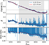 |
Fig. A.1. PSF parameters fitted across wavelength. The values obtained when using stacks of 12.5 Åare used as constraining prior for the wavelength-by-wavelength fit. The shaded area indicates the range of wavelength used for the σLOS measurement, and the dotted lines highlight the mean value of the parameters in this range. |
A.2. Is the lens rotating?
To investigate bias in the σLOS measurement due to possible rotation of the lens galaxy, we designed three spatial masks cutting half of the lens light area as shown in the left panel of A.2. The three masks are chosen to ensure an equivalent S/N for the three configurations while minimising the spatial overlap. With the same methodology as described in Section 4.2, we then measured the line-of-sight velocity of each bin  . The bottom panel of Fig.A.2 shows that there is no sign of ordered rotation. These observations are, hence, consistent with the assumption that the lens galaxy is a slow rotator.
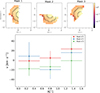 |
Fig. A.2. Top panel: three different masked MUSE cube cutouts. Bottom panel: measured velocity of the three bins in each case. |
Appendix B: MUSE by-products
B.1. Spectra extracted from the MUSE data
We present here the spectra of the center of the lens galaxy (S/N ∼ 30Å−1), perturbers P5 (∼ 11Å−1), P6 (∼ 7Å−1), and images A (∼ 529Å−1) and B (∼ 266Å−1) of the quasar extracted at the positions displayed in Fig.4.
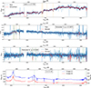 |
Fig. B.1. Integrated spectra from the MUSE data cube with apertures shown in Fig. 4. The binned flux is computed by imposing a minimal S/N of 5 per wavelength bin. From top to bottom, Lens centre: from left to right, the stellar absorption lines CaH, CaK, H[[INLINE557]], and G-band (orange dashed lines) are consistent with the previously determined zd = 0.729. P5: from left to right, the galactic emission lines Ne III, He I, H[[INLINE559]], and H[[INLINE560]] are highlighted with green dashed lines and allowed us to measure z5 = 0.3575. We also identify the stellar absorption lines H[[INLINE562]], HEI, CaH, and CaK allowing a velocity dispersion measurement. P6: from left to right the lines Mg I, Ca II O II, H[[INLINE563]], and O III doublet allowed us to measure z6 = 0.505. Quasar images: from left to right, we recognise the C IV, C III, C II, and Mg II emission lines. |
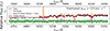 |
Fig. B.2. Measurement of the P5 stellar kinematics. Point-estimate of σLOSP5. |
B.2. Velocity dispersion of the perturber P5
We applied the same stellar template fitting process as performed with the lens galaxy spectra to the spectrum of P5 shown in Fig. B.1. In this case, we used the observed wavelength range [(4600,4700):(5600,5700)] Å. As shown by Fig. B.2, the absorption lines are not altered by the sky but by galactic gas emission lines. We thus incorporated those in the model without testing different masks. We obtained the  . According to Knabel et al. (2025), spectra with relatively low S/N, such as this one, may be affected by systematic bias up to ∼4%, which is negligible compared to the uncertainty of the measurement.
Appendix C: Lens modelling, additional material
C.1. PSF reconstruction for HST imaging
The Fig.C.1 shows the PSF obtained after the iterative reconstruction procedure described in Section 6.2.4.
C.2. Image reconstruction
We now show the decomposition of the imaging reconstruction, i.e. the lens light and source light obtained with a power-law in Fig.C.2 and composite in Fig. C.3 models.
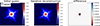 |
Fig. C.1. From left to right: Initial guess of the PSF from stacked stars in the field, final PSF obtained, and the difference between both. |
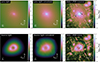 |
Fig. C.2. HE 1104−1805 reconstructed light component with power-law. From left to right: The light component unconvolved, convolved with the PSF, and its corresponding feature in the imaging data. The top row shows the lens light profile, and the bottom row shows the lensed source light profile. This figure shows that the light-components model corresponds to expectations based on the observation. The centre of the PSF and of the lens are not ideally modelled, which justifies the noise map increase in the first region and the masking of the second region. |
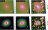 |
Fig. C.3. HE 1104−1805 reconstructed light component with power-law. From left to right: The light component unconvolved and then convolved with the PSF and its corresponding feature in the imaging data. The top row shows the lens light profile, and the bottom row shows the lensed source light profile. This figure shows that the light-components model corresponds to expectations based on the observation. The centre of the PSF and of the lens are not ideally modelled, which justifies the noise map increase in the first region and the masking of the second region. |
Appendix D: Galaxy perturber groups members
Fig. D.1 displays the position and velocities of the galaxy groups included as perturbers in the lens model.
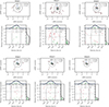 |
Fig. D.1. Galaxy groups identified in the spectroscopic sample of galaxies in the field of HE 1104−1805. For each group, the upper plot shows the positions of the candidate member galaxies associated with that group relative to the lens galaxy, with rejected group members represented as red squares and accepted group members represented as green circles. The lens galaxy (star) and group centroid (cross) are also displayed. The R200 radius of the group is represented by a solid line, while the dashed circle represents the angular separation cut of the group-finding algorithm in its final iteration. The lower plot shows the observer-frame velocity of individual member galaxies relative to the group centroid as a function of that galaxy’s angular distance from the centroid. Galaxies that passed the iterative algorithm described in Buckley-Geer et al. (2020), Sluse et al. (2017), and Sluse et al. (2019) are shown in green, while trial galaxy members that were cut through the algorithm are shown in red. Horizontal error bars represent the measurement error for each galaxy. The final observer-frame velocity dispersion and angular separation cuts from the group-finding algorithm are presented as dashed and dotted lines, respectively. We also show 1-D histograms and rug plots of the velocity and distance distributions of the member galaxies. The 1-D histograms are produced using a kernel density estimate (KDE) with a bandwidth determined using Scott’s Rule. In the 1D velocity histogram, the dashed blue line shows a Gaussian with a width equal to the observer-frame velocity dispersion of the group. |
All Tables
Summary of lens modelling scenarios and their relative weight within each family.
All Figures
|
Fig. 1. Left panel: Stack of 280 WFI exposures of the field of view used for light curve extraction. Stars nominated PSF1 to PSF5 are used to model the PSF of each exposure, and stars designated as N1 to N5 are used to normalise the flux between each exposure. Right panel: HE 1104−1805 imaging in the filter F160W band using HST WFC3. The main lensing galaxy is denoted as G, whereas the main perturbers within 5″ of the lens are numbered from P1 to P9. |
| In the text | |
|
Fig. 2. Top panel: HE 1104−1805 R-band light curve obtained by joining three datasets: SMARTS (yellow and blue squares), ECAM (purple and green circles), and WFI (brown and pink triangles). For clarity, the light curve of B was shifted by –1.05 mag. The inset zooms on the WFI dataset span, showcasing its superior sampling to the ECAM dataset. Bottom panel: Example of a simultaneous fit of an intrinsic light curve with η = 45 days and nml = 15. The time shift obtained by this fit gives a point estimate of the system’s time delay. By repeating such measurements with randomised starting points 800 times, we obtained the time-delay measurement of this (η, nml) configuration. |
| In the text | |
|
Fig. 3. Left panel: Measurements of the time delay for different configurations of (η, nml) with the merged ECAM+SMART+WFI dataset. Right panel: Measurement of ΔtAB for the different datasets. Since the datasets overlap, they cannot be considered fully independent. We therefore use our estimate on the joint dataset ECAM+SMARTS+WFI (green data point) as our final estimate. In both panels, the ‘combined τ = 0.5’ value was obtained by marginalising over the measurements listed above it. |
| In the text | |
|
Fig. 4. MUSE data cube summed over all wavelengths. The inset displays the point-source subtracted cube, revealing the lens galaxy light. The apertures used to extract individual spectra of the quasar images, lens centre, and perturbers shown in Fig. B.1 are represented by orange circles. |
| In the text | |
|
Fig. 5. Velocity dispersion point-estimate in the three radial bins of HE 1104−1805’s lens galaxy. Left panel: Mean of the MUSE data cube after PSF subtraction and masking with overlaid bin numbers and contours. Right panel: Example of a pPXF fit of the integrated spectra of each bin, where data masked for the fit are marked in grey. |
| In the text | |
|
Fig. 6. Wide-field imaging of HE 1104−1805 in the i-band. Red circles denote regions within 8″, 45″ and 120″ of the centre of the lens. |
| In the text | |
|
Fig. 8. κext measurement showing that the line-of-sight of HE 1104−1805 is along a slightly underdense region of the Universe. Therefore, the fact that multiple perturbers are near the main lens is coincidental and the approximation κext ≈ κs holds. |
| In the text | |
|
Fig. 7. Position and weight (size of the dot) of galaxies between us and the source. Black circles indicate the 45″ and 120″ apertures. Blue dots correspond to objects with i-magnitudes less than 24. |
| In the text | |
|
Fig. 9. Reconstructed image of HE 1104−1805 using the best power-law and composite models. From left to right: The imaging data, reconstructed image, and normalised residuals are displayed for the power law model (PEMD + Shear + perturbers 2, 5, 6, 9 + groups 1, 2, 3, and 4) and composite models (NFW + Double chameleon + Shear + perturbers 2, 5, 6, 9 + groups 1, 2, 3, and 4). |
| In the text | |
|
Fig. 10. HE 1104−1805 modelled convergence κ with the two families of models and different perturbers and groups inclusion strategies. The top row shows a wide-field including all groups and the bottom row zooms in on the region closer to the main lens; white lines indicate the area enclosing 25, 50, and 75% of the total mass. |
| In the text | |
|
Fig. 11. BIC weighted comparison of the power-law and composite models. For each family, we marginalised over the three posteriors given by the three perturber inclusion scenarios, which results in the multi-modality of some of the parameters such as γ. We obtained |
| In the text | |
|
Fig. 12. Left panel: Kinematic fit using power-law and composite models. Red and blue central dots show the best-fit values, while error bars are the 16th and 84th percentiles of 100 predicted velocity dispersions. Right panel: Posterior of Dd and DΔt using kinematics based on the power-law and composite mass models. Using likelihood weighting we measured |
| In the text | |
|
Fig. 13. H0 measurement with HE 1104−1805 using the joint constraint of DΔt and Dd measured with the power-law, composite models, and both models combined. Our final measurement using the likelihood weighted combination of both models is |
| In the text | |
|
Fig. A.1. PSF parameters fitted across wavelength. The values obtained when using stacks of 12.5 Åare used as constraining prior for the wavelength-by-wavelength fit. The shaded area indicates the range of wavelength used for the σLOS measurement, and the dotted lines highlight the mean value of the parameters in this range. |
| In the text | |
|
Fig. A.2. Top panel: three different masked MUSE cube cutouts. Bottom panel: measured velocity of the three bins in each case. |
| In the text | |
|
Fig. B.1. Integrated spectra from the MUSE data cube with apertures shown in Fig. 4. The binned flux is computed by imposing a minimal S/N of 5 per wavelength bin. From top to bottom, Lens centre: from left to right, the stellar absorption lines CaH, CaK, H[[INLINE557]], and G-band (orange dashed lines) are consistent with the previously determined zd = 0.729. P5: from left to right, the galactic emission lines Ne III, He I, H[[INLINE559]], and H[[INLINE560]] are highlighted with green dashed lines and allowed us to measure z5 = 0.3575. We also identify the stellar absorption lines H[[INLINE562]], HEI, CaH, and CaK allowing a velocity dispersion measurement. P6: from left to right the lines Mg I, Ca II O II, H[[INLINE563]], and O III doublet allowed us to measure z6 = 0.505. Quasar images: from left to right, we recognise the C IV, C III, C II, and Mg II emission lines. |
| In the text | |
|
Fig. B.2. Measurement of the P5 stellar kinematics. Point-estimate of σLOSP5. |
| In the text | |
|
Fig. C.1. From left to right: Initial guess of the PSF from stacked stars in the field, final PSF obtained, and the difference between both. |
| In the text | |
|
Fig. C.2. HE 1104−1805 reconstructed light component with power-law. From left to right: The light component unconvolved, convolved with the PSF, and its corresponding feature in the imaging data. The top row shows the lens light profile, and the bottom row shows the lensed source light profile. This figure shows that the light-components model corresponds to expectations based on the observation. The centre of the PSF and of the lens are not ideally modelled, which justifies the noise map increase in the first region and the masking of the second region. |
| In the text | |
|
Fig. C.3. HE 1104−1805 reconstructed light component with power-law. From left to right: The light component unconvolved and then convolved with the PSF and its corresponding feature in the imaging data. The top row shows the lens light profile, and the bottom row shows the lensed source light profile. This figure shows that the light-components model corresponds to expectations based on the observation. The centre of the PSF and of the lens are not ideally modelled, which justifies the noise map increase in the first region and the masking of the second region. |
| In the text | |
|
Fig. D.1. Galaxy groups identified in the spectroscopic sample of galaxies in the field of HE 1104−1805. For each group, the upper plot shows the positions of the candidate member galaxies associated with that group relative to the lens galaxy, with rejected group members represented as red squares and accepted group members represented as green circles. The lens galaxy (star) and group centroid (cross) are also displayed. The R200 radius of the group is represented by a solid line, while the dashed circle represents the angular separation cut of the group-finding algorithm in its final iteration. The lower plot shows the observer-frame velocity of individual member galaxies relative to the group centroid as a function of that galaxy’s angular distance from the centroid. Galaxies that passed the iterative algorithm described in Buckley-Geer et al. (2020), Sluse et al. (2017), and Sluse et al. (2019) are shown in green, while trial galaxy members that were cut through the algorithm are shown in red. Horizontal error bars represent the measurement error for each galaxy. The final observer-frame velocity dispersion and angular separation cuts from the group-finding algorithm are presented as dashed and dotted lines, respectively. We also show 1-D histograms and rug plots of the velocity and distance distributions of the member galaxies. The 1-D histograms are produced using a kernel density estimate (KDE) with a bandwidth determined using Scott’s Rule. In the 1D velocity histogram, the dashed blue line shows a Gaussian with a width equal to the observer-frame velocity dispersion of the group. |
| In the text | |
Current usage metrics show cumulative count of Article Views (full-text article views including HTML views, PDF and ePub downloads, according to the available data) and Abstracts Views on Vision4Press platform.
Data correspond to usage on the plateform after 2015. The current usage metrics is available 48-96 hours after online publication and is updated daily on week days.
Initial download of the metrics may take a while.