| Issue |
A&A
Volume 706, February 2026
|
|
|---|---|---|
| Article Number | A273 | |
| Number of page(s) | 18 | |
| Section | Cosmology (including clusters of galaxies) | |
| DOI | https://doi.org/10.1051/0004-6361/202556442 | |
| Published online | 16 February 2026 | |
Measuring the intergalactic medium correlation length at 5 < z < 6.1: A fast change at the end of reionization
1
Institute for Theoretical Physics, Heidelberg University Philosophenweg 12 D–69120 Heidelberg, Germany
2
Max-Planck-Institut für Astronomie Königstuhl 17 69117 Heidelberg, Germany
★ Corresponding author: This email address is being protected from spambots. You need JavaScript enabled to view it.
Received:
16
July
2025
Accepted:
30
November
2025
Abstract
Context. The Lyman-α forest of high-redshift quasars is a powerful probe of the late stages of the epoch of reionization (EoR), in particular thanks to the presence of Gunn-Peterson troughs. These troughs exhibit a broad range of lengths, with some extending up to ∼100 cMpc, suggesting large-scale coherent structures in the intergalactic medium (IGM).
Aims. We aim to gain more insight into the presence, extent, and magnitude of correlations in the Lyman-α forest at the end of reionization, at 5 < z < 6.1. In particular, we want to quantify the scales over which correlations are significant in order to help inform the required size of cosmological simulations aiming to capture the evolution of the EoR.
Methods. We utilized the extended XQR-30 observational dataset over the redshift range 5 < z < 6.1 (Δz = 0.05) to explore large-scale correlations. After accounting for the relevant systematics, the flux correlation matrix proved to be a powerful tool for probing large-scale correlations across redshifts. We performed a Monte Carlo Markov chain analysis to quantify the extent and strength of the correlation, making use of several functional forms. We moreover employed new large-volume (1.53 Gpc3) light cones of Lyman-α transmission implementing different reionization scenarios to interpret the observed signal, including a fiducial box employing SCRIPT.
Results. We detected strong correlations at redshifts z > 5.3, extending at least tens of megaparsecs and strongly increasing with redshift. Our results suggest a redshift-dependent correlation length, from L ≤ 26.53 (68.47) Mpc at 1σ (2σ) limit at redshift z = 5.0 to L = 252.72+272.61−41.61 Mpc at redshift z = 6.1. On the contrary, our simulations all demonstrate characteristic correlation scales < 60 Mpc with a very slow redshift evolution, in strong tension with our observations.
Conclusions. The presence and redshift dependence of correlations in the Lyman-α forest on > 200 Mpc scales at z = 6 indicates that cosmological simulations should be larger than this scale to adequately sample the Lyman-α forest. Despite implementing a fluctuating ultraviolet background and numerous neutral islands at z < 6, and matching well the sightline scatter in the Lyman-α forest, our fiducial SCRIPT-based simulation fails to reproduce the large-scale correlations. It may be that those ingredients are necessary, but insufficient, to understand the unfolding of the EoR.
Key words: intergalactic medium / quasars: general / cosmology: observations / dark ages / reionization / first stars
© The Authors 2026
 Open Access article, published by EDP Sciences, under the terms of the Creative Commons Attribution License (https://creativecommons.org/licenses/by/4.0), which permits unrestricted use, distribution, and reproduction in any medium, provided the original work is properly cited.
This article is published in open access under the Subscribe to Open model. This email address is being protected from spambots. You need JavaScript enabled to view it. to support open access publication.
1. Introduction
The epoch of reionization (EoR) marks the last major global phase transition in the history of the Universe. During this period, the intergalactic medium (IGM) gradually became ionized while structures formed, making the study of the EoR crucial for understanding IGM physics and galaxy formation in the early Universe.
The midpoint of the EoR is set at redshift z ∼ 7 − 8 by observations of the cosmic microwave background (Planck Collaboration VI 2020), the decline of Lyman-α emission from galaxies at z > 6 (Mason et al. 2018; Jung et al. 2020; Wold et al. 2022), the analyses of the Lyman-α damping wing in quasars at z ≥ 7 (Wang et al. 2020; Yang et al. 2020b; Greig et al. 2022), and the IGM thermal state measurements at z > 5 (Gaikwad et al. 2020, 2021). It is in this context that the analysis of high-quality spectra obtained from high-redshift quasars (QSOs) emerges as an essential tool to probe the timeline of the EoR and its end in particular, starting with the measurement of the fraction of dark pixels in the Lyman series forests (McGreer et al. 2015; Davies et al. 2026).
Although substantial sightline-to-sightline variations in Lyman-α optical depth can arise from a decline in the ionizing background, even without a significantly neutral IGM (Lidz et al. 2006; Bolton & Haehnelt 2007; Davies & Furlanetto 2016; D’Aloisio et al. 2018), the observed scatter exceeds expectations from cosmic density fluctuations alone (Becker et al. 2015; Bosman et al. 2018; Yang et al. 2020a; Zhu et al. 2021; Bosman et al. 2022), suggesting a late and patchy reionization scenario and placing the end of the EoR at z ≃ 5.3 (Kulkarni et al. 2019; Nasir & D’Aloisio 2020; Keating et al. 2020). This picture is also supported by the rapid evolution of the mean free path of ionizing photons at 5 < z < 6 (Becker et al. 2021; Bosman 2021; Zhu et al. 2023), and the underdensities around long gaps traced by Lyman-α emitting galaxies (Becker et al. 2018; Christenson et al. 2023).
A key constraint provided by the Lyman-α forest arises from the Gunn-Peterson (GP) effect – the absorption of rest-frame (wavelength of 1215.67 Å) quasar photons by neutral hydrogen (Gunn & Peterson 1965), with an HI fraction xHI ≳ 10−4 along the line of sight to background quasars – leading to the so-called GP troughs. In particular, the detection of an extended (∼110 h−1 Mpc) trough in ULAS J0148+0600 (Becker et al. 2015) challenged the previously held scenario that reionization ended around z ∼ 6 and highlighted the potential of GP troughs to probe the final stages of the EoR. Since GP troughs appear even for very low xHI (Mesinger 2010), their presence alone does not distinguish between residual neutral gas and large, significantly neutral islands. However, the detection of damping wings around GP troughs in the Lyman-α forest of z < 6 quasars (Spina et al. 2024; Zhu et al. 2024) suggests that substantial neutral hydrogen persisted late.
Gunn–Peterson troughs have been detected with sizes extending for tens of comoving megaparsecs (cMpc), indicating extended coherent neutral regions in the IGM and implying the presence of correlations on scales approaching 100 cMpc. Such large coherent regions point to specific physical mechanisms driving the late stages of the EoR and place constraints on the nature of the ionizing sources and the topology of reionization. From a practical perspective, they also raise important questions regarding the fidelity of numerical simulations with box sizes smaller than these scales in capturing the relevant IGM correlations. The purpose of this work is to quantify the characteristic correlation scale of the IGM and to assess the implications for both the underlying reionization physics and the requirements for simulation volumes needed to model it accurately.
The idea that the reionization process affects and has structure on all scales was shown in Furlanetto & Oh (2016) with an analysis of the EoR through percolation theory, but without quantifying strength or impact, i.e., whether it would be detectable. Whether ∼100 cMpc simulations are sufficient for the convergence of key reionization features (such as the size and distribution of ionized bubbles) is extensively discussed in Gnedin & Madau (2022), suggesting the need for simulations larger than 250 cMpc. The issue of convergence in simulation boxes – and, more broadly, the correlation of scales – has been poorly explored from a theoretical perspective, and it remains almost unaddressed in observations. The first attempt to do so appears in Fan et al. (2006a,b), where the evolution of the IGM optical depth is investigated and large fluctuations in the UV background are reported, implying that transmission is correlated over large scales. By accounting for the redshift evolution across different sightline bins in a sample of 19 quasars, they reported a correlation scale of tens of comoving megaparsecs. From a theoretical perspective, similar conclusions were reached by Battaglia et al. (2013), by measuring the power spectrum of the ionization field in large-scale EoR simulations, and by Qin et al. (2021) cross-correlating the overdensity field with the Lyman-α transmission flux. Previous attempts (e.g., Croft & Altay 2008) to quantify the correlation of scales introduced by the reionization process have been limited by the small volume accessible from high-resolution simulations and have been mainly focused on estimating the size and distribution of ionized bubbles (Furlanetto et al. 2006; Furlanetto & Mesinger 2009). Studies on the Lyman-α forest flux autocorrelation function at z ≥ 5 (Wolfson et al. 2024) have pointed out significant correlations at small scales (on the order of a few megaparsecs), without addressing larger scales. Zhu et al. (2021), on the other hand, focus on the occurrence rates of GP troughs larger than 30 h−1 Mpc alone, which are rare, especially at z < 5.5. In contrast, we address the correlation scales on the transmission directly.
We aim to provide a systematic study of the optical depth correlation toward the end of the EoR using high-resolution QSO spectra at high redshift from the E-XQR-30 quasar sample (D’Odorico et al. 2023), obtained with the X-Shooter instrument (Vernet et al. 2011, installed at the ESO-VLT telescope) and ESI (Sheinis et al. 2002, installed at the Keck II telescope) instruments. The sample is fully described in Bosman et al. (2022).
The paper is organized as follows. In Section 2, we describe our observational sample, detailing the continuum-reconstruction procedure and addressing key systematics in the data. Our methodology is outlined in Section 3 and it includes the data preparation for fitting (Section 3.1) and the functional forms employed (Section 3.2). We present and analyze our results in Section 4. In Section 5 we introduce and investigate the simulations used to interpret our findings, followed by the discussion and conclusions in Section 6. The cleaned and binned QSO spectra are shown in Appendix A, while details on the Monte Carlo Markov chain (MCMC) posteriors are shown in Appendix D, and further comparisons between data, models, and simulations are displayed in Appendix E. Throughout the paper we use a Planck flat Λ cold dark matter (ΛCDM) cosmology (Planck Collaboration VI 2020), and distances are given in comoving units.
2. Sample
We used 67 QSO spectra at redshift z > 5.5, with signal-to-noise ratios (S/Ns) of ≥10 per ≤15 km s−1 spectral pixel (Bosman et al. 2022). We combined observations from the X-Shooter and ESI instruments in order to increase our sample size and improve the statistical analysis.
For each sightline, the flux was binned into redshift bins of Δz = 0.05 in the redshift range 4.975 ≤ z ≤ 6.125 (the redshift bins are therefore centered at zbin = 5.00, 5.05, …, 6.10), covering the last stage of the EoR and entering the post-EoR regime. We adopted Δz = 0.05 bins to resolve the diffuse correlation signal without introducing excess noise from small-scale fluctuations. We show in Appendix B results obtained with finer (Δz = 0.01) and coarser (Δz = 0.05) redshift bins.
We included non-detections in our sample as well (the flux is hence allowed to be negative), since both the observational uncertainties and the uncertainties related to the continuum-reconstruction are available and well behaved. The redshift bins for which the Lyman-α forest is available are peculiar to each QSO, and as was expected, not all the QSOs contribute to all the redshift bins. In particular, the redshift bins closer to the edges of our redshift range are under-sampled with respect to the central bins. It also implies that not all of the redshift combinations (i.e. redshift 5 with redshift 6) provides constraints with the same robustness. We applied the same masking on the blue side of the Lyman-α emission line – to account for proximity zone contamination – as in Bosman et al. (2022), excluding rest-frame wavelengths of λ > 1185 Å. Damped Lyman-α systems (DLAs) identified along quasar sightlines (Davies et al. 2023) are masked. A more detailed description of the sample and the data-cleaning procedures (e.g., masking of residuals from sky emission lines) can be found in Bosman et al. (2022).
In addition, we removed those redshifts that might be contaminated by the OVI doublet emission line (λλ1032, 1038 Å), i.e., closer than Δv = 5000 km s−1 from the OVI redshifted peak. This conservative mask reduces the redshift bins available for the analysis but robustly prevents any contamination that might introduce artificial correlations, since OVI is a more difficult emission line to reconstruct in quasar spectra than the other lines in the wavelength range we use (Bosman et al. 2021). The effects of the masking are shown in Appendix A, along with the wavelengths used for the analysis.
The full sample is presented in Figure A.1. For each quasar, the binned flux is presented in black as a function of redshift (the shaded gray region represents the continuum-reconstruction error) and the data selected by accounting for the OVI doublet emission line (vertical semi-dashed light blue line) in red. The Lyman-α and Lyman-β lines are also displayed as the dashed orange and dotted blue lines, respectively.
The Lyman-α forest of each quasar was normalized by reconstructing the continuum flux using a near-linear log-PCA method (Davies et al. 2018; Bosman et al. 2021, 2022). This approach has been shown to predict the underlying continuum within an ∼8% uncertainty for each quasar, though this uncertainty is highly coherent (i.e., the entire continuum can be systematically under- or overestimated). To account for this uncertainty, we simulated the effect of the continuum-reconstruction using mock observations of the Lyman-α forest from Davies et al. (2024). The mock observations consists of 1000 independent realizations of the QSO sample presented in Bosman et al. (2022). Furthermore, they are tailored to match the observed sample, for example in terms of the number of quasars contributing to each redshift bin, and were obtained by interpolating the original redshift binning of Δz = 0.1 to the redshift binning used in this work, Δz = 0.05. Specifically, for each redshift and each quasar in the mock sample, the continuum-normalized flux is perturbed by a factor of 1 + 𝒢(σz, QSOcont), where 𝒢(σz, QSOcont) is a random number drawn from a Gaussian distribution with a standard deviation specific to each quasar at each redshift (measured in Bosman et al. 2022), representing the uncertainty on continuum reconstruction. This approach carefully and accurately models the continuum-reconstruction process by systematically varying the flux across redshift bins, enabling the generation of realistic mock spectra that reflect observational properties. It is worth noting that by applying this procedure we are conservatively assuming a complete error correlation across all scales, slightly overestimating by ∼10%, on purpose, the error introduced by the continuum reconstruction on large scales.
3. Methods
We aim to investigate and quantify the strength and extent of Lyman-α forest correlations on different scales. We achieve this by measuring the correlation between combinations of redshift bins and evaluating its statistical significance, accounting for systematics such as continuum reconstruction and observational uncertainties.
3.1. Correlation matrix
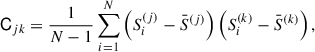
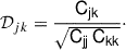
As a first step, we computed the correlation matrix, 𝒟, of the sightlines described in Sect. 2, shown in the top left panel of Figure 1. Let Si denote the flux transmission field along the i-th QSO sightline, discretized into M redshift bins, with i = 1, …, N and N = 67 the total number of sightlines considered. We computed the sample mean,  , for each redshift bin, the elements of the covariance matrix, Cjk (where j, k = 1, …, M denote the redshift bins), and the elements of the correlation matrix, 𝒟jk, of the sightline ensemble as follows:
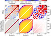 |
Fig. 1. Correlations in the Lyman-α forest flux across redshift. Top row: Correlation matrix for observed QSO sightlines, showing a positive correlation (in red) in the off-diagonal terms near the diagonal at all redshifts, and an increasing correlation length at higher redshifts. Bottom row: Mock sightlines with continuum-reconstruction uncertainties applied, leading to a slight increase in correlation at lower redshifts, while failing to account for the observed correlation at higher redshifts. First column: Correlation matrices. Second column: Standard deviation of the correlation matrices. Third column: Statistical significance of the correlation, estimated as the ratio between the correlation matrix and its standard deviation. The results suggest that while continuum-reconstruction uncertainties contribute to correlations at low redshifts, they cannot account for the correlations observed at higher redshifts. |
 (1)
(1)
 (2)
(2)
 (3)
(3)
A positive correlation is consistently observed at all redshifts in the off-diagonal terms near the diagonal and even in more distant terms at higher redshifts, suggesting that correlations extend not only between neighboring bins but also across redshift separations of up to δz ∼ 0.5. An enhanced correlation at high redshift would imply a scale-coherent behavior of the IGM during the late stages of the EoR, indicating a more interconnected structure than in the post-reionization era.
For comparison with more conventional statistical formulations, we show in Appendix C the covariance matrix, C, normalized by  , which is equivalent to the standard autocorrelation function. This formulation, however, is highly sensitive to the steep evolution of the mean flux and is therefore not well suited for measuring the correlation length over the redshift range considered in this work.
However, whether this correlation is statistically significant remains to be determined, as it could arise from systematic effects, such as those introduced by the continuum-reconstruction (here conservatively assumed to be fully correlated). To assess the strength of the signal, we shuffled the flux in the sightlines by randomly permuting the flux values across sightlines within each redshift bin N = 1000 times and computed the standard deviation of the correlation matrices produced in each shuffling, effectively computing the standard deviation of 𝒟, σ𝒟, presented in the top middle panel of Figure 1. As was previously noted, the number of QSOs contributing to each redshift combination decreases toward the edges of the considered redshift range, resulting in a higher standard deviation in these regimes. A first, approximate yet informative measure of the statistical significance of the correlation is given by the ratio between the correlation matrix and its standard deviation, as is shown in the top right panel of Figure 1. A S/N of ≥2 correlation is visible in the off-diagonal terms near the diagonal across all redshifts, with increasing correlation length at higher redshifts. Meanwhile, the apparent correlation between very low redshifts (e.g., z = 5) and very high ones (e.g., z = 5.7), due to the size of our sample and observed in the top left panel, appears not to be statistically significant.
In order to account for the impact of the continuum reconstruction uncertainties, we repeated the same procedure using the mock observations of the Lyman-α forest described in Sect. 2, shown in the second row of Figure 1. These mock sightlines contain no intrinsic correlation across scales, apart from the one introduced by the continuum-reconstruction correlated uncertainties, as is shown in their correlation matrix 𝒞. A mild correlation appears at redshifts z ∼ 5.0 − 5.5 with a persistent and correlated S/N ∼ 0.4 in the bottom left panel of Figure 1 when introducing the continuum uncertainties. Its statistical significance, σ𝒞, is displayed in the bottom middle panel of Figure 1.
While uncertainties in continuum-reconstruction may account for the observed correlation in the off-diagonal terms at low redshifts, they do not explain the correlation seen at higher redshifts. To assess the extent of this contribution, we repeated the continuum-reconstruction procedure described in Section 2, by artificially increasing the uncertainty on the continuum reconstruction measured in Bosman et al. (2022), denoted as σz, QSOcont. While being confident about the accuracy of the reconstruction, we allowed for the measured uncertainties to be underestimated by 50% and we tested the sensitivity to the continuum-reconstruction uncertainty of our results. As was expected, this led to an enhancement of the correlation at low redshifts (S/N ∼0.8), consistent with the trend already visible in the bottom left panel of Figure 1. However, this modification had no apparent effect on the correlation at higher redshifts (consistent within 10%), reinforcing the robustness of our results against systematic errors.
The correlation matrix and the covariance matrix normalized by  were also computed for finer (Δz = 0.01) and coarser (Δz = 0.1) redshift bins in Appendix B and Appendix C respectively. In the former case, the large-scale correlations are dominated by local effects and only small scales correlations emerge; in the latter case, while a strong correlation is visible at large separations, the coarse bins prevents the correlation length from being estimated precisely.
3.2. Fitting through functional forms
The correlation matrix analysis in Section 3.1 reveals a strong correlation at high redshift, which we now aim to quantify and model. Ideally, the continuum-fitting uncertainties would be forward modelled within the simulations, but this is not currently feasible given the empirical nature of the continuum reconstruction and would not yield additional insight at this stage. Instead, as a pragmatic approximation, we computed the difference between the correlation matrices of the data, 𝒟, and of the mock sightlines including the continuum uncertainty, 𝒞. This subtraction isolated the intrinsic IGM correlation by removing the additive bias introduced by continuum reconstruction. Observational uncertainties are an order of magnitude smaller than continuum errors and largely uncorrelated across redshift, and are therefore neglected. The resulting correlation matrix, ℱ = 𝒟 − 𝒞, forms the basis for testing different models of the correlation scale.
We considered three functional forms to model the signal we detected,
-
ℳ1
-
A constant model, preferred if there is no correlation between scales.
-
ℳ2
A Gaussian model, with a fixed amplitude and width. It will be statically preferred over ℳ1 if correlations are present. In this model, the characteristic correlation scale does not depend on redshift (i.e., scales are correlated at a fixed distance). The functional form depends on the comoving distance between z1 and z2.
-
ℳ3
A Gaussian model, as ℳ2, but with redshift-dependent amplitude and width; in this case, the correlation length is not fixed but depends on the redshift considered. It will be preferred over ℳ2 if there is statistically significant evidence of a redshift dependence of the characteristic correlation scale.
We used MCMC methods to explore the parameter space and fit different models to the correlation matrix, ℱ. We performed the MCMC sampling using the emcee package (Foreman-Mackey et al. 2013). We used the reciprocal of each term of the standard deviation matrix, σ𝒟, to compute the diagonal terms of the inverted covariance matrix, required for the likelihood evaluation. This approach ensures proper weighting of the data uncertainties while fitting the correlation model.
In the following, we present the functional forms and the results of the fitting in Table 1 and Figures 2a, 2b, and 2c (while the posterior distributions and contours can be found in Appendix D). Each figure shows the correlation matrix used for the fitting, ℱ (top left panel), the model resulting from the best fit, ℳ (top right panel), the residuals between the two, ℱ − ℳ (bottom left panel), and the S/N, (ℱ − ℳ)/σ𝒟 (bottom right panel). In the top left panel, isocontours corresponding to the difference of the comoving distances at each redshift pair (i.e., χ(z1)−χ(z2), in units of megaparsecs) are also shown. The functional form for each model, the best fit, and the minimum χ2 are shown in Table 1.
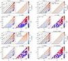 |
Fig. 2. Results of the fitting for different models. For each model, we show in the top left panel the correlation matrix used for the fitting, obtained by removing the effects from the continuum-reconstruction from the data; isocontours corresponding to the comoving distances in megaparsecs at each redshift pair are also shown. The top right panel displays results from the best fitting of the model considered here, ℳ. The residuals between the data and the best fit of the model, ℱ − ℳ, are shown in the bottom left panel. Finally, the bottom right panel shows the S/N of the data. Analogous panels for the simulations BIBORTON constλ and evolvλ are displayed in Figure E.3. Panel (a): Model ℳ1; constant. Panel (b): Model ℳ2; Gaussian, constant amplitude and width. Panel (c): Model ℳ3; Gaussian, amplitude and width redshift-dependent. Panel (d): BIBORTON SCRIPT. |
3.3. χ2 evaluation
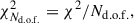
To evaluate the goodness of fit for each model and compare between models, we considered the χ2 distribution and its minimum, minχ2. The number of degrees of freedom is listed in Table 1 and defined as
 (4)
(4)
where Nd.o.f., 𝒟 = 221 represents the number of independent redshift bin pairs in the correlation matrix, 𝒟, and Θℳ the number of free parameters in each model, ℳ. The models we tested have only a few free parameters (Θℳ ≤ 4), ensuring that Nd.o.f., 𝒟 ≫ Θℳ. We quantified the significance of the improvement in the fit between models using the likelihood ratio test (Wilks 1938), where the difference in χ2 values between two models is asymptotically distributed as a χ2 distribution with degrees of freedom equal to the difference of the models degrees of freedom. For example, a Δχ2 = 10 with ΔNd.o.f. = 2 (1) degree of freedom corresponds to an improvement in the fit of a 2.5σ (2.9σ) significance.
We also made use of the reduced χ2,
 (5)
(5)
and its minimum minχNd.o.f.2, which accounts for the number of degrees of freedom and is expected to be close to unity for a statistically consistent model under Gaussian errors, to evaluate the goodness of fit.
To compare models with different numbers of free parameters, it is also useful to consider the Akaike information criterion (AIC, Akaike 1974), which penalizes over-parameterization while rewarding good fits (reported in the last column of Table 1). For a model with Θℳ free parameters and a χ2 goodness of fit, the AIC is defined as
 (6)
(6)
A lower AIC indicates a model that achieves a better balance between goodness of fit and model complexity.
4. Data fitting via models, ℳ
We tested our data against three functional forms of increasing complexity (Section 3.2), designed to capture the interplay between different scales. We present our findings in the following. A summary of the model definition, the best fits obtained via the MCMC and the minimum χ2, is listed in Table 1.
Summary of models and their best-fit parameters.
The simplest model, ℳ1, assumes no scale-dependent correlation and, as was expected, provides the poorest fit to the data (χNd.o.f.2 ℳ1 = 1.35, AICℳ1 = 300.4). In particular, it fails to reproduce the observed correlation between nearby redshift bins, which gradually decreases with separation at low redshift while strengthening at higher redshift. Nonetheless, the amplitude constrained by fitting the model to the data, 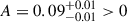 , seems to suggest a mild but significant overall correlation.
Model ℳ2 assumes a strong correlation between nearby redshift bins that decays with separation. It is implemented as a Gaussian function centered on the diagonal of the correlation matrix, parameterized by the comoving separation of each redshift pair, with a constant amplitude and width. This model successfully captures the extent of correlation at low redshifts (see the bottom left panel of Figure 2b, which shows the residuals between the data and the model) but fails to reproduce the increasing strength of correlation at higher redshifts. The parameter L in the functional form adopted (see Table 1) represents the characteristic correlation length. The best-fit values obtained via MCMC are  and
and 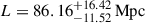 , indicating correlations between scales around 90 Mpc apart. The correlation length obtained for this model is also shown in Figure 3 as a continuous light blue line. The comparison of the minimum χ2 values between the constant model ℳ1 and the Gaussian model with constant amplitude and width ℳ2 strongly favors the latter (
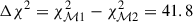 , with an improvement of 6.4σ significance). The improvement in the fitting is marked by a reduced χ2 of χNd.o.f.2 ℳ2 = 1.17 (χNd.o.f.2 ℳ1 = 1.35, also AICℳ1 = 300.4 while AICℳ2 = 260.6).
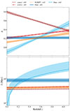 |
Fig. 3. Amplitude (top panel) and correlation length (bottom panel) as a function of redshift for different models and simulations. The continuous light blue (blue) lines are the results of fitting the observations with ℳ2 (ℳ3), a Gaussian model with constant (redshift-dependent) width and amplitude. The shaded regions represent the 1σ error on the A (L) parameters. The shaded blue region instead indicates the 16th and 84th percentiles of the A0-A1 (L0-L1) joint-posterior distribution, except for redshifts of z < 5.1, where only the 1σ upper limit of L is shown. The dashed brown, dash-dotted red, and dotted orange lines are the results of fitting the simulations (const λ, evolv λ, SCRIPT) with ℳ3. |
Only our last model ℳ3, Gaussian with a redshift-dependent amplitude and width, is able to capture the correlation at high redshifts and allow us to provide an estimate of its strength and length. For a fixed redshift, z1, the Gaussian profile evolves with z2 through its amplitude and width, both of which are allowed to vary linearly with z2 (see Table 1). This additional flexibility enables ℳ3 to better describe the evolution of correlations across redshifts. The residuals, shown in the bottom left panel of Figure 2c, demonstrate a significantly improved fit, particularly at high redshift. The posterior distribution (see Figure D.1c in Appendix D) shows a well-constrained amplitude of  , mildly evolving with redshift. The width, however, defined as L(z1, z2) = L0 + L1 ⋅ (z2 − 5), is less tightly constrained: while its evolution with redshift is well recovered in the MCMC run (through the L1 parameter), its constant counterpart (L0) is constrained only as an upper limit. The best-fit parameters read L0 ≤ 76.45 Mpc at the 2σ level and
  , suggesting a combination of a general, overall, correlation with a strong, redshift-dependent one. The correlation scale, L, as a function of redshift is shown in Figure 3 as a continuous blue curve, representing the maximum likelihood from the joint posterior distribution of the L0 and L1 parameters at each redshift. The shaded region indicates the 16th and 84th percentiles of these distributions, except for redshifts z < 5.1, where only an upper limit of L is shown. Our results suggest a redshift-dependent correlation length, from L ≤ 26.53 (68.47) Mpc at 1σ (2σ) at redshift z = 5.0 to
 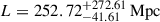 at redshift z = 6.1.
The best-fit χ2 obtained from the fitting procedure is 202.9, corresponding to a reduced χ2 of χNd.o.f.2 ℳ3 = 0.94 ∼ 1, strongly favoring ℳ3 over ℳ2 (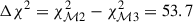 , with an improvement of 7σ significance). The AIC is 210.9 (AICM2 = 260.6).
In summary, all models detect correlations in the Lyman-α forest flux across redshift, with their inferred strength and scale depending on the model. The best-fit χ2 (and reduced χ2) is achieved with our most general function, ℳ3, which includes a redshift-dependent correlation length, suggesting coherent structures extending over ≳200 Mpc at the highest redshifts, z > 6. The resulting best-fit correlation scales as a function of redshift are shown in Figure 3.
Finally, in order to be as conservative as possible, we repeated the analysis, while allowing for a possible underestimation of the uncertainties arising from continuum flux reconstruction, which are correlated across all scales. To do this, we perturbed each quasar in the mock sample by a factor of 1 + 𝒢(1.5 ⋅ σz, QSOcont), i.e., with a increase of 50% in the uncertainties compared to the analysis above, and far more pessimistic than the accuracy measurements for the PCA-based reconstruction method we were employing. The results are shown in Figure F.1. The measurement of L(z) when increasing the continuum-reconstruction error by 50% are consistent within 10% with the fiducial analysis above.
5. Simulations
To gain insights into the physical processes occurring during the late EoR, we wish to compare our observational findings with physically motivated IGM simulations. For this study, we would ideally require a simulation box with a high dynamic range that preserves large-scale correlations while simultaneously capturing the small scale physics. However, that is unfortunately computationally intractable with currently available resources. Instead, we used a complementary method and employed an optimized approach using a semi-numerical technique developed by Maity et al. (2026). This method can efficiently generate large-volume lightcones of Ly-α transmission across the redshift range (z = 4.9 − 6.2, separated by a comoving length of ∼420 h−1 Mpc) relevant to our study. Below, we briefly summarize the simulation procedures of the BIBORTON (BIg BOxes for ReionizaTiON) suite of simulations that will be fully described in Maity et al. (in prep.).
In the semi-numerical setup, the Ly-α optical depth is assumed to depend on underlying cosmological density fluctuations, ultraviolet background (UVB) fluctuations, temperature fluctuations, and ionization fluctuations (if reionization is incomplete). These dependencies are calibrated against a high-resolution full hydrodynamic simulation (in this case Nyx, Almgren et al. 2013). Additionally, the semi-numerical reionization and UVB generation models require information on the collapsed halo mass fraction (fcoll) to quantify available ionizing sources. For the purpose of this work, we generated density fields with a large box size (L) of 1024 h−1 Mpc at a given redshift using the Zel’Dovich approximation (Zel’dovich 1970), while the collapsed fraction field was generated using excursion set formalism in Lagrangian space (ESF-L; Trac et al. 2022). This provides sufficient resemblance with full N-body simulations at large scales, while allowing us to efficiently investigate the EoR evolution. We worked with a spatial resolution (Δx) of 4 h−1 Mpc, allowing for an optimization between efficiency and accuracy. To get the lightcone evolution, we generated the boxes at a redshift interval of Δz = 0.1 and interpolated the redshifts in between. Given the density and source information, we utilized the EX-CITE model (Gaikwad et al. 2023) to efficiently generate UVB fluctuations, while incorporating local source contributions following Davies & Furlanetto (2016), Davies et al. (2024). This approach requires two input parameters: the effective mean free path of ionizing photons (λmfp) and the mean photoionization rate (⟨ΓHI⟩). Furthermore, ionization and temperature evolution were modeled using the photon-conserving reionization model, SCRIPT, which accounts for recombination effects (Choudhury & Paranjape 2018; Maity & Choudhury 2022). In this study, we did not explicitly include radiative feedback for computational convenience; instead, we accounted for its effects by imposing a constant threshold halo mass (Mmin = 109 M⊙), below which collapsed objects cannot form. We explored three different scenarios, which are listed below:
-
constλmfp: BIBORTON with constant λmfp: In this case, we assumed a constant mean free path (λmfp = 11.94 Mpc, Maity et al. 2026) throughout the redshift range for UVB generation. We further assumed that the reionization is over at redshift z ≥ 6.1 (i.e., no neutral island is left in the redshift range considered in this work) and the temperature was estimated using the standard power law relation with density, T = T0Δγ − 1 (with T0 = 104K and γ = 1.35, Maity et al. 2026).
-
evolvλ: BIBORTON with evolving λmfp: This is similar to the previous model except we now allowed for redshift-dependent evolution of λmfp. Specifically, we assumed a linear variation from 5.97 Mpc at z = 6.2 to 37.31 Mpc at z = 4.9.
-
SCRIPT: BIBORTON with SCRIPT (fiducial): This case incorporates a realistic reionization scenario (with reionization ending at z ≈ 5.7 and a neutral island present until this moment) generated with SCRIPT, as was described earlier. This model now incorporates self-consistent temperature fluctuations satisfying IGM temperature estimates (Gaikwad et al. 2020). The evolution of λmfp is assumed to be same as the previous one. The underlying matter density, the normalized photo-ionization rate, the flux, the temperature evolution, and the HI fraction for this model are shown in Figure 4.
In each of these cases, we tuned the mean photoionization rate at each redshift to match the observed distribution of mean transmission fluxes (Bosman et al. 2022). Once all the necessary fields were generated, we then constructed the lightcone volume for the redshift range studied in this work. Notably, the lightcones are not affected by any correlations coming from boundary discontinuities as our box size is large enough to cover the whole comoving length corresponding to the redshift range of our interest. Finally, we extracted 1000 random line-of-sight skewers that we used for the correlation-scale analysis.
In order to properly compare the random skewers extracted from the simulations with the observations, observational noise must be incorporated into the former. We achieved this by perturbing each simulated skewer at each redshift. Specifically, for each skewer, we randomly selected a quasar from the observed sample and, at each redshift, added a random noise component drawn from a Gaussian distribution 𝒢(σz, QSOobs) with a standard deviation, σz, QSOobs, equal to the observational uncertainty of the chosen quasar at that redshift. Given that the observational uncertainties were not correlated across redshift, each redshift in the simulated skewer was perturbed independently using the corresponding uncertainty of the selected quasar. Since the continuum-reconstruction uncertainties were accounted for at the observation level by subtracting their contribution from the observed correlation matrix (Section 3), we did not correct the simulations for the continuum-reconstruction procedure. This procedure ensures that the simulated skewers closely mimic the statistical properties of real observations, while preserving the underlying large-scale correlations.
5.1. Correlation matrix
We computed the correlation matrix for the 1000 random skewers extracted from lightcones in the BIBORTON simulation suite. The resulting correlation matrices, their standard deviations (each obtained by building N = 1000 correlation matrices of 67 random sightlines tailored to reproduce the observational sample), and their significance, are shown in the columns of Figure 5 (the autocorrelation is reported in Appendix C). Each row represents one of the lightcones of the simulation suite (constλ, evolvλ, SCRIPT). Interestingly, the correlation between redshift bins exhibited in the lightcones is consistently weaker than the one observed in the data. A mild correlation between nearby redshift bins is visible for a constant λmfp = 11.94 Mpc (constλ), both at high and low redshift, slightly increasing toward higher redshifts. In evolvλ, the mean free path evolves from λmfp = 5.97 Mpc at z = 6.2 to λmfp = 37.31 Mpc at z = 4.9 (i.e., λmfp(z = 5.95) = 11.94 Mpc); the correlation is lower then for constλ at high redshift, but remains comparable at low ones (where the mean free path is approximately triple), in line with the mild correlation at low redshift observed in the data. The last simulation, SCRIPT, has the same mean free path evolution of evolvλ but later ending of reionization (z ≈ 5.7); a broader, but weaker with respect to constλ and evolvλ, correlation is detected at all redshifts.
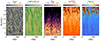 |
Fig. 4. Lightcone from BIBORTON simulations, with SCRIPT model (SCRIPT, see Section 5). From left to right, we show the underlying matter density, the normalized photo-ionization rate, the flux, the temperature, and the HI fraction. The lightcone fully covers the redshift range considered in this work and has a size of ∼1.5 cGpc. |
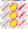 |
Fig. 5. Same as Figure 1, but for the BIBORTON simulations. Note the different ranges of color for the second and third columns. |
5.2. Modeling through BIBORTON simulations
The simple functional forms presented in Section 3.2 provide a clear interpretation and measure of the correlation length, either through the parameter L or its absence. Once such a correlation has been estimated, we aim to explore the underlying physical processes responsible for setting the observed correlation scale. For this reason, we compared the observations with the BIBORTON simulations, each representing a different model for the late stages of the EoR. In particular, both constλ and evolvλ assume an early-ending reionization scenario (z ≥ 6.1); in the former, the mean free path, λmfp, is held constant, whereas in the latter it is allowed to evolve with time. Meanwhile, SCRIPT incorporates a more realistic reionization history, ending at z ≈ 5.7 (with neutral islands present until then). The results are presented in Figure 2d for our fiducial simulation SCRIPT, in Figures E.3a and E.3b for the other models, and summarized in Table 1.
None of the simulations, however, successfully reproduce the observed correlations. While the behavior at low redshift is generally recovered (the residuals normalized by the standard deviation are in general consistent with zero and randomly distributed), the residual panels in each figure reveal a lack of correlation strength at high redshift. The poor fit is further confirmed by the χ2 and reduced χNd.o.f.2 values, which yield for constλ and evolvλ values of χNd.o.f.2 constλ = 392.3/221 = 1.76 and χNd.o.f.2 evolvλ = 278.8/221 = 1.26. This is furthermore confirmed by the corresponding AIC, of 392.3 and 278.8, respectively. The fiducial simulation SCRIPT shows the best agreement with observations (χNd.o.f.2 SCRIPT = 274.6/221 = 1.24, AICSCRIPT = 274.6), presenting a broad but weak correlation at all scales (but failing to reproduce the high-redshift one). This is despite the fact that all three simulations match the observed distribution of Lyman-α transmission at these redshifts, meaning that high optical depth in the forest is not sufficient to reproduce the correlations we observed.
We tested how our most general model, ℳ3, fit the simulations. As a Gaussian model with a redshift-dependent amplitude and width, ℳ3 can, in principle, reproduce both ℳ1 (which corresponds to no correlation, i.e., L ∼ 0 Mpc or considerably small) and ℳ2 (which assumes a redshift-independent correlation, i.e., L1 ∼ 0 Mpc). We present the results of this fit in Figures E.1, E.2 and Table 1, while the evolution of the correlation length with redshift is shown in Figure 3.
The model captures the main features of the lightcones, yielding minimum χ2 values that are generally higher than those obtained for the observational fits, though still comparable (χNd.o.f.2 constλ − ℳ3 = 1.23, χNd.o.f.2 evolvλ − ℳ3 = 1.45, χNd.o.f.2 SCRIPT − ℳ3 = 1.36). It is similar for the AIC (AICconstλ − ℳ3 = 269.8, AICevolvλ − ℳ3 = 323.4, AICSCRIPT − ℳ3 = 302.8).
The constraints on the free parameters differ significantly from those obtained in the observations. For instance, the redshift-dependent component of the amplitude, A1, is now constrained to be negative for constλ (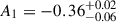 ), leading to an overall decreasing amplitude with redshift. The amplitude parameter, A, recovered for each simulation and when fitting the data is shown in the top panel of Figure 3. The amplitude recovered when fitting the data with ℳ3, strongly increases with redshift, while it has a milder evolution for constλ and evolvλ simulations.
The main difference, however, concerns the correlation length: a weak redshift dependence is now preferred over a strong one, with L1 consistent with zero in all cases. The correlation length recovered in each simulation is generally around ∼50 Mpc, much lower than the one recovered by fitting the data with the same model (spanning from 50 Mpc at low redshift to 250 Mpc at high redshift). The amplitude and correlation lengths constrained with the simulations, as a function of redshift, are shown in Figure 3 as the dashed brown line (constλ), the dash-dotted red line (evolvλ), and the dotted orange line (SCRIPT). The shaded regions are computed as the 16th and 84th percentiles of the A0-A1 and L0-L1 joint-posterior distribution.
For constλ, the simulation with constant mean free path, the correlation length suggested by fitting ℳ3 has a very weak dependence on redshift, going from 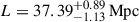 at redshift z = 5.0 to
 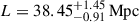 at redshift z = 6.1. A strong (S/N ≥3) correlation is detected between nearby redshift bins, with a scale of ∼3 times the constant mean free path implemented in the simulation.
When allowing the mean free path to vary with redshift (spanning from ∼6 Mpc to ∼37 Mpc), as for the simulation evolvλ, the correlation length results higher than for constλ, spanning from 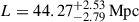 at redshift z = 5.0 to
  at redshift z = 6.1. Correlations with a S/N ≥2 are strongly detected between nearby redshift bins but only in the central redshift interval (∼5.3 − 5.8). The short mean free path implemented at high redshift does not allow the ionizing photons to causally connect more distant regions. Finally, postponing the end of the EoR to z ≈ 5.7 (i.e., introducing neutral islands) has a similar effect, leading to a correlation length of
  at redshift z = 5.0 to
  at redshift z = 6.1.
6. Summary and conclusion
The existence of GP troughs over 100 Mpc in length at z ≥ 5.7 signals the fact that the ionization state of the IGM is potentially correlated on scales far larger than the density field (Becker et al. 2015). We used 67 Lyman-α forest skewers including the E-XQR-30 dataset to quantify these correlation scales at 5.0 < z < 6.1 and investigate potential redshift evolution.
The normalized covariance matrix of the Lyman-α flux, computed in bins of Δz = 0.05, is shown in Figure 1. After carefully accounting for systematics as is described in Section 3, we find statistically significant correlations on extremely large scales: the transmitted flux at z = 5.6 is positively correlated with all higher redshifts along the same skewers.
We fit the correlation matrix and its uncertainties with a function describing a redshift-independent Gaussian correlation in redshift (ℳ2), finding a best-fit characteristic scale of 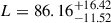 Mpc. This simple model is strongly preferred over a model with no correlation between redshifts (ℳ1): the minimum (reduced) χ2 drops from 298.4 to 256.6 (1.35 to 1.17) with the addition of one extra parameter.
Next, we allowed the Gaussian correlation scale to vary linearly with redshift (ℳ3), finding again a statistically significant improvement with the minimum (reduced) χ2 dropping to 202.9 (0.94) by adding two free parameters. The recovered characteristic correlation scales increase from L < 76.45 Mpc at z = 5.0 (2σ limit) to 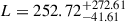 Mpc at z = 6.1. In other words, at z = 6.1, the Lyman-α forest is correlated on scales no smaller than 200 Mpc: far larger than typical numerical (and semi-numerical) models of the reionization process.
To explore whether semi-numerical models of the density field and reionization are able to reproduce correlations on such scales, we used the recent BIBORTON simulation framework (Maity et al. 2026). This suite uses a simulation of the density field in a very large box, 1024 h−1 Mpc on the side, onto which UVB fluctuations are added using EX-CITE (Gaikwad et al. 2023). We generated lightcones spanning the same redshift range as the observations, forward-modeled Lyman-α forest skewers, and computed the covariance matrix in the same way as for the observed dataset. We find that three versions of BIBORTON, assuming either a constant mean free path or an evolving mean free path, or fully processed through SCRIPT, all display significantly shorter correlation scales than the observations and provide a worse fit than our simple assumption of a redshift-independent Gaussian correlation (ℳ2) Despite the fact that they match the observed mean flux and scatter of the Lyman-α forest, the BIBORTON simulations all have characteristic correlation scales of < 60 cMpc at z = 6, in strong tension with our observations, by a factor of over four.
A correlation scale in excess of 100 Mpc is perhaps not surprising in the context of the existence of large GP troughs at z > 5.5 (Becker et al. 2015); however, such troughs are still rare at z < 6 (Zhu et al. 2021), so additional correlations within the transmissive regions of the IGM may still be required to explain our measurement. A hint of the excess correlations on large scales can be seen in autocorrelation function measurements of Wolfson et al. (2024): while they only considered scales up to L ∼ 15 cMpc (the size of our individual flux bins), they generally found indications of elevated large-scale correlations compared to simulations.
A potential explanation for these discrepancies lies in the reionization models implemented in the simulations. Both constλ and evolvλ assume an early and uniform end to reionization, with no surviving neutral islands at the redshifts of interest. While this could initially be considered a reason for the lack of correlation, SCRIPT, which includes neutral islands persisting to lower redshifts, still does not match the observations. This suggests that the presence of UVB fluctuations and neutral structures alone do not explain the observed correlation trends.
Furthermore, an evolving mean free path of ionizing photons does not seem, by itself, to significantly affect correlation strength, as is shown by the similarity in correlation behavior between constλ and evolvλ. Interestingly, in SCRIPT, where neutral islands persist, the correlation strength is lower than in evolvλ at redshifts where reionization is still ongoing. This suggests a complex relationship between the mean free path, neutral islands, and large-scale correlations.
Future z > 6 quasars to be soon discovered by Euclid (Euclid Collaboration: Mellier et al. 2025) and followed up on by ELT/ANDES (D’Odorico et al. 2024; Marconi et al. 2024) will enable a more precise characterization of large-scale IGM correlations. Euclid’s wide-area coverage will increase the number of high-z quasars, while the ELT will be able to deliver high-S/N spectra of these fainter sources. Potentially, the number of known quasars during the end of the EoR may one day be sufficiently large to enable the search for transverse correlations between sightlines in addition to the purely longitudinal ones considered in this work.
Data availability
The correlation matrix of the QSO sightlines computed and used in this work is available at the CDS via https://cdsarc.cds.unistra.fr/viz-bin/cat/J/A+A/706/A273
Acknowledgments
BS and SEIB are supported by the Deutsche Forschungsgemeinschaft (DFG) under Emmy Noether grant number BO 5771/1-1. Part of this work is based on observations collected at the European Southern Observatory under ESO programme 1103.A-0817. We thank Andrei Mesinger, Anna Pugno and Elena Marcuzzo for the useful comments and discussions.
References
- Akaike, H. 1974, IEEE Trans. Automat. Control, 19, 716 [Google Scholar]
- Almgren, A. S., Bell, J. B., Lijewski, M. J., Lukić, Z., & Van Andel, E. 2013, ApJ, 765, 39 [NASA ADS] [CrossRef] [Google Scholar]
- Battaglia, N., Trac, H., Cen, R., & Loeb, A. 2013, ApJ, 776, 81 [NASA ADS] [CrossRef] [Google Scholar]
- Becker, G. D., Bolton, J. S., Madau, P., et al. 2015, MNRAS, 447, 3402 [Google Scholar]
- Becker, G. D., Davies, F. B., Furlanetto, S. R., et al. 2018, ApJ, 863, 92 [NASA ADS] [CrossRef] [Google Scholar]
- Becker, G. D., D’Aloisio, A., Christenson, H. M., et al. 2021, MNRAS, 508, 1853 [NASA ADS] [CrossRef] [Google Scholar]
- Bolton, J. S., & Haehnelt, M. G. 2007, MNRAS, 382, 325 [NASA ADS] [CrossRef] [Google Scholar]
- Bosman, S. E. I. 2021, ArXiv e-prints [arXiv:2108.12446] [Google Scholar]
- Bosman, S. E. I., Fan, X., Jiang, L., et al. 2018, MNRAS, 479, 1055 [Google Scholar]
- Bosman, S. E. I., Ďurovčíková, D., Davies, F. B., & Eilers, A.-C. 2021, MNRAS, 503, 2077 [CrossRef] [Google Scholar]
- Bosman, S. E. I., Davies, F. B., Becker, G. D., et al. 2022, MNRAS, 514, 55 [NASA ADS] [CrossRef] [Google Scholar]
- Choudhury, T. R., & Paranjape, A. 2018, MNRAS, 481, 3821 [NASA ADS] [CrossRef] [Google Scholar]
- Christenson, H. M., Becker, G. D., D’Aloisio, A., et al. 2023, ApJ, 955, 138 [Google Scholar]
- Croft, R. A. C., & Altay, G. 2008, MNRAS, 388, 1501 [Google Scholar]
- D’Aloisio, A., McQuinn, M., Davies, F. B., & Furlanetto, S. R. 2018, MNRAS, 473, 560 [CrossRef] [Google Scholar]
- Davies, F. B., & Furlanetto, S. R. 2016, MNRAS, 460, 1328 [NASA ADS] [CrossRef] [Google Scholar]
- Davies, F. B., Hennawi, J. F., Bañados, E., et al. 2018, ApJ, 864, 142 [NASA ADS] [CrossRef] [Google Scholar]
- Davies, R. L., Ryan-Weber, E., D’Odorico, V., et al. 2023, MNRAS, 521, 289 [NASA ADS] [CrossRef] [Google Scholar]
- Davies, F. B., Bosman, S. E. I., Gaikwad, P., et al. 2024, ApJ, 965, 134 [NASA ADS] [CrossRef] [Google Scholar]
- Davies, F. B., Bosman, S. E. I., D’Odorico, V., et al. 2026, MNRAS, 542, 1862 [Google Scholar]
- D’Odorico, V., Bañados, E., Becker, G. D., et al. 2023, MNRAS, 523, 1399 [CrossRef] [Google Scholar]
- D’Odorico, V., Bolton, J. S., Christensen, L., et al. 2024, Exp. Astron., 58, 21 [Google Scholar]
- Euclid Collaboration (Mellier, Y., et al.) 2025, A&A, 697, A1 [Google Scholar]
- Fan, X., Carilli, C. L., & Keating, B. 2006a, ARA&A, 44, 415 [Google Scholar]
- Fan, X., Strauss, M. A., Becker, R. H., et al. 2006b, AJ, 132, 117 [NASA ADS] [CrossRef] [Google Scholar]
- Foreman-Mackey, D., Hogg, D. W., Lang, D., & Goodman, J. 2013, PASP, 125, 306 [Google Scholar]
- Furlanetto, S. R., & Mesinger, A. 2009, MNRAS, 394, 1667 [Google Scholar]
- Furlanetto, S. R., & Oh, S. P. 2016, MNRAS, 457, 1813 [NASA ADS] [CrossRef] [Google Scholar]
- Furlanetto, S. R., McQuinn, M., & Hernquist, L. 2006, MNRAS, 365, 115 [Google Scholar]
- Gaikwad, P., Rauch, M., Haehnelt, M. G., et al. 2020, MNRAS, 494, 5091 [Google Scholar]
- Gaikwad, P., Srianand, R., Haehnelt, M. G., & Choudhury, T. R. 2021, MNRAS, 506, 4389 [NASA ADS] [CrossRef] [Google Scholar]
- Gaikwad, P., Haehnelt, M. G., Davies, F. B., et al. 2023, MNRAS, 525, 4093 [NASA ADS] [CrossRef] [Google Scholar]
- Gnedin, N. Y., & Madau, P. 2022, Liv. Rev. Comput. Astrophys., 8, 3 [CrossRef] [Google Scholar]
- Greig, B., Mesinger, A., Davies, F. B., et al. 2022, MNRAS, 512, 5390 [NASA ADS] [CrossRef] [Google Scholar]
- Gunn, J. E., & Peterson, B. A. 1965, ApJ, 142, 1633 [Google Scholar]
- Jung, I., Finkelstein, S. L., Dickinson, M., et al. 2020, ApJ, 904, 144 [NASA ADS] [CrossRef] [Google Scholar]
- Keating, L. C., Weinberger, L. H., Kulkarni, G., et al. 2020, MNRAS, 491, 1736 [NASA ADS] [CrossRef] [Google Scholar]
- Kulkarni, G., Keating, L. C., Haehnelt, M. G., et al. 2019, MNRAS, 485, L24 [Google Scholar]
- Lidz, A., Oh, S. P., & Furlanetto, S. R. 2006, ApJ, 639, L47 [Google Scholar]
- Maity, B., & Choudhury, T. R. 2022, MNRAS, 511, 2239 [NASA ADS] [CrossRef] [Google Scholar]
- Maity, B., Davies, F., & Gaikwad, P. 2026, A&A, 706, A36 [NASA ADS] [CrossRef] [EDP Sciences] [Google Scholar]
- Marconi, A., Abreu, M., Adibekyan, V., et al. 2024, SPIE Conf. Ser., 13096, 1309613 [Google Scholar]
- Mason, C. A., Treu, T., Dijkstra, M., et al. 2018, ApJ, 856, 2 [Google Scholar]
- McGreer, I. D., Mesinger, A., & D’Odorico, V. 2015, MNRAS, 447, 499 [NASA ADS] [CrossRef] [Google Scholar]
- Mesinger, A. 2010, MNRAS, 407, 1328 [Google Scholar]
- Nasir, F., & D’Aloisio, A. 2020, MNRAS, 494, 3080 [Google Scholar]
- Planck Collaboration VI. 2020, A&A, 641, A6 [NASA ADS] [CrossRef] [EDP Sciences] [Google Scholar]
- Qin, Y., Mesinger, A., Bosman, S. E. I., & Viel, M. 2021, MNRAS, 506, 2390 [NASA ADS] [CrossRef] [Google Scholar]
- Sheinis, A. I., Bolte, M., Epps, H. W., et al. 2002, PASP, 114, 851 [Google Scholar]
- Spina, B., Bosman, S. E. I., Davies, F. B., Gaikwad, P., & Zhu, Y. 2024, A&A, 688, L26 [NASA ADS] [CrossRef] [EDP Sciences] [Google Scholar]
- Trac, H., Chen, N., Holst, I., Alvarez, M. A., & Cen, R. 2022, ApJ, 927, 186 [NASA ADS] [CrossRef] [Google Scholar]
- Vernet, J., Dekker, H., D’Odorico, S., et al. 2011, A&A, 536, A105 [NASA ADS] [CrossRef] [EDP Sciences] [Google Scholar]
- Wang, F., Davies, F. B., Yang, J., et al. 2020, ApJ, 896, 23 [NASA ADS] [CrossRef] [Google Scholar]
- Wilks, S. S. 1938, Ann. Math. Stat., 9, 60 [Google Scholar]
- Wold, I. G. B., Malhotra, S., Rhoads, J., et al. 2022, ApJ, 927, 36 [NASA ADS] [CrossRef] [Google Scholar]
- Wolfson, M., Hennawi, J. F., Bosman, S. E. I., et al. 2024, MNRAS, 531, 3069 [NASA ADS] [CrossRef] [Google Scholar]
- Yang, J., Wang, F., Fan, X., et al. 2020a, ApJ, 897, L14 [Google Scholar]
- Yang, J., Wang, F., Fan, X., et al. 2020b, ApJ, 904, 26 [Google Scholar]
- Zel’dovich, Y. B. 1970, A&A, 5, 84 [NASA ADS] [Google Scholar]
- Zhu, Y., Becker, G. D., Bosman, S. E. I., et al. 2021, ApJ, 923, 223 [NASA ADS] [CrossRef] [Google Scholar]
- Zhu, Y., Becker, G. D., Christenson, H. M., et al. 2023, ApJ, 955, 115 [CrossRef] [Google Scholar]
- Zhu, Y., Becker, G. D., Bosman, S. E. I., et al. 2024, MNRAS [Google Scholar]
Appendix A: QSO sample
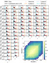 |
Fig. A.1. Fig. A.1: Quasar sample, as described in Sec. 2. Each quasar is displayed in a different panel, ordered by redshift, with a binning of Δz = 0.05. The detected flux as a function of redshift is shown as a black continuous line. The gray shaded region represents the continuum-reconstruction uncertainty. Data selected based on the OVI doublet emission line (semi-dashed light blue vertical line) are highlighted in red. The Lyman-α and Lyman-β lines are indicated by the dashed orange and dotted blue lines, respectively. The number of sightlines available in each redshift bin (and their combination) is reported in the bottom right panel. |
Appendix B: Alternative redshift bins
We have tested alternative redshift binnings of Δz = 0.01 and 0.1, recomputing the correlation matrix as in Fig. 1. With a finer binning (Δz = 0.01), small-scale correlations dominate the signal and obscure the large-scale component. Conversely, a coarser binning (Δz = 0.1) enhances the visibility of large-scale correlations but reduces the resolution, preventing a precise estimate of the correlation length. We therefore adopt Δz = 0.05 as a compromise between resolution and S/N.
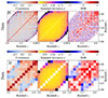 |
Fig. B.1. Same as Fig. 1 but with a finer (top) redshift binning (Δz = 0.01) and a coarser (bottom) redshift binning (Δz = 0.1). |
Appendix C: Normalized covariance
For comparison with more conventional statistical formulations, we also present the covariance matrix C normalized by  , which corresponds to the standard autocorrelation function. This quantity is shown for the finer (Fig. C.2), standard (Fig. C.1), and coarser (Fig. C.3) redshift binnings, as well as for the BIBORTON simulation suite (Fig. C.4). However, this formulation is highly sensitive to the steep evolution of the mean flux and is therefore not optimal for measuring the correlation length across the redshift range considered here.
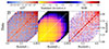 |
Fig. C.1. Covariance matrix, C, normalized by the mean flux |

Appendix D: Fitting the data: Models’ MCMC posteriors
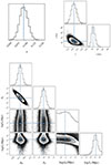 |
Fig. D.1. Posterior and best fit from the MCMC for the different models. Panel (a): constant model, ℳ1; panel (b): gaussian model with constant amplitude and width, ℳ2; panel (c): gaussian model with redshift-dependent amplitude and width, ℳ3 (for convenience, L0 and L1 are sampled logarithmically). |
Appendix E: Comparing simulations with the observations and model ℳ3
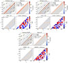 |
Fig. E.1. As Figure 2, but here the different simulations are fitted with model ℳ3. Panel (a): simulation constλ fitted with model ℳ3; panel (b): simulation evolvλ fitted with model ℳ3; panel (c): simulation SCRIPT fitted with model ℳ3. |
 |
Fig. E.2. Posterior distribution for Figure E.1, where the different simulations are fitted with model ℳ3. Panel (a): simulation constλ fitted with model ℳ3; panel (b): simulation evolvλ fitted with model ℳ3; panel (c): simulation SCRIPT fitted with model ℳ3. |
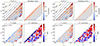 |
Fig. E.3. As Figure 2 for BIBORTON constλ and evolvλ simulations. Panel (a): BIBORTON simulation with constant λmfp; panel (b): BIBORTON simulation with an evolving with redshift λmfp. |
Appendix F: Underestimated continuum-reconstruction error
All Tables
All Figures
|
Fig. 1. Correlations in the Lyman-α forest flux across redshift. Top row: Correlation matrix for observed QSO sightlines, showing a positive correlation (in red) in the off-diagonal terms near the diagonal at all redshifts, and an increasing correlation length at higher redshifts. Bottom row: Mock sightlines with continuum-reconstruction uncertainties applied, leading to a slight increase in correlation at lower redshifts, while failing to account for the observed correlation at higher redshifts. First column: Correlation matrices. Second column: Standard deviation of the correlation matrices. Third column: Statistical significance of the correlation, estimated as the ratio between the correlation matrix and its standard deviation. The results suggest that while continuum-reconstruction uncertainties contribute to correlations at low redshifts, they cannot account for the correlations observed at higher redshifts. |
| In the text | |
|
Fig. 2. Results of the fitting for different models. For each model, we show in the top left panel the correlation matrix used for the fitting, obtained by removing the effects from the continuum-reconstruction from the data; isocontours corresponding to the comoving distances in megaparsecs at each redshift pair are also shown. The top right panel displays results from the best fitting of the model considered here, ℳ. The residuals between the data and the best fit of the model, ℱ − ℳ, are shown in the bottom left panel. Finally, the bottom right panel shows the S/N of the data. Analogous panels for the simulations BIBORTON constλ and evolvλ are displayed in Figure E.3. Panel (a): Model ℳ1; constant. Panel (b): Model ℳ2; Gaussian, constant amplitude and width. Panel (c): Model ℳ3; Gaussian, amplitude and width redshift-dependent. Panel (d): BIBORTON SCRIPT. |
| In the text | |
|
Fig. 3. Amplitude (top panel) and correlation length (bottom panel) as a function of redshift for different models and simulations. The continuous light blue (blue) lines are the results of fitting the observations with ℳ2 (ℳ3), a Gaussian model with constant (redshift-dependent) width and amplitude. The shaded regions represent the 1σ error on the A (L) parameters. The shaded blue region instead indicates the 16th and 84th percentiles of the A0-A1 (L0-L1) joint-posterior distribution, except for redshifts of z < 5.1, where only the 1σ upper limit of L is shown. The dashed brown, dash-dotted red, and dotted orange lines are the results of fitting the simulations (const λ, evolv λ, SCRIPT) with ℳ3. |
| In the text | |
|
Fig. 4. Lightcone from BIBORTON simulations, with SCRIPT model (SCRIPT, see Section 5). From left to right, we show the underlying matter density, the normalized photo-ionization rate, the flux, the temperature, and the HI fraction. The lightcone fully covers the redshift range considered in this work and has a size of ∼1.5 cGpc. |
| In the text | |
|
Fig. 5. Same as Figure 1, but for the BIBORTON simulations. Note the different ranges of color for the second and third columns. |
| In the text | |
|
Fig. A.1. Fig. A.1: Quasar sample, as described in Sec. 2. Each quasar is displayed in a different panel, ordered by redshift, with a binning of Δz = 0.05. The detected flux as a function of redshift is shown as a black continuous line. The gray shaded region represents the continuum-reconstruction uncertainty. Data selected based on the OVI doublet emission line (semi-dashed light blue vertical line) are highlighted in red. The Lyman-α and Lyman-β lines are indicated by the dashed orange and dotted blue lines, respectively. The number of sightlines available in each redshift bin (and their combination) is reported in the bottom right panel. |
| In the text | |
|
Fig. B.1. Same as Fig. 1 but with a finer (top) redshift binning (Δz = 0.01) and a coarser (bottom) redshift binning (Δz = 0.1). |
| In the text | |
|
Fig. C.1. Covariance matrix, C, normalized by the mean flux |
| In the text | |
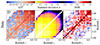 |
Fig. C.2. Same as Fig. C.1, but with a standard redshift binning (Δz = 0.05) |
| In the text | |
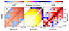 |
Fig. C.3. Same as Fig. C.1, but with a coarser redshift binning (Δz = 0.1) |
| In the text | |
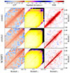 |
Fig. C.4. Same as Fig. C.1 for the BIBORTON simulations. |
| In the text | |
|
Fig. D.1. Posterior and best fit from the MCMC for the different models. Panel (a): constant model, ℳ1; panel (b): gaussian model with constant amplitude and width, ℳ2; panel (c): gaussian model with redshift-dependent amplitude and width, ℳ3 (for convenience, L0 and L1 are sampled logarithmically). |
| In the text | |
|
Fig. E.1. As Figure 2, but here the different simulations are fitted with model ℳ3. Panel (a): simulation constλ fitted with model ℳ3; panel (b): simulation evolvλ fitted with model ℳ3; panel (c): simulation SCRIPT fitted with model ℳ3. |
| In the text | |
|
Fig. E.2. Posterior distribution for Figure E.1, where the different simulations are fitted with model ℳ3. Panel (a): simulation constλ fitted with model ℳ3; panel (b): simulation evolvλ fitted with model ℳ3; panel (c): simulation SCRIPT fitted with model ℳ3. |
| In the text | |
|
Fig. E.3. As Figure 2 for BIBORTON constλ and evolvλ simulations. Panel (a): BIBORTON simulation with constant λmfp; panel (b): BIBORTON simulation with an evolving with redshift λmfp. |
| In the text | |
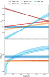 |
Fig. F.1. Same as Figure 3 but increasing the uncertainty on the continuum-reconstruction by 50%. |
| In the text | |
Current usage metrics show cumulative count of Article Views (full-text article views including HTML views, PDF and ePub downloads, according to the available data) and Abstracts Views on Vision4Press platform.
Data correspond to usage on the plateform after 2015. The current usage metrics is available 48-96 hours after online publication and is updated daily on week days.
Initial download of the metrics may take a while.