| Issue |
A&A
Volume 706, February 2026
|
|
|---|---|---|
| Article Number | A12 | |
| Number of page(s) | 12 | |
| Section | Numerical methods and codes | |
| DOI | https://doi.org/10.1051/0004-6361/202556476 | |
| Published online | 28 January 2026 | |
SPT-GloCal: Enhancing [O/Fe] and [Mg/Fe] determinations in metal-poor stars with UV-extended low-resolution CSST spectra
1
School of Mathematics and Statistics, Shandong University,
Weihai
264209,
Shandong,
PR China
2
CAS Key Lab of Optical Astronomy, National Astronomical Observatories,
Chinese Academy of Sciences A20 Datun Road, Chaoyang,
Beijing
100101,
PR China
3
School of Astronomy and Space Science, University of Chinese Academy of Sciences,
Beijing
100049,
PR China
4
School of Physics and Technology, Nantong University,
Nantong
226019,
PR China
5
School of Space Science and Technology, Shandong University,
Weihai
264209,
PR China
6
School of Airspace Science and Engineering, Shandong University,
Weihai
264209,
PR China
★ Corresponding author: This email address is being protected from spambots. You need JavaScript enabled to view it.
Received:
18
July
2025
Accepted:
28
November
2025
Abstract
Metal-poor stars (MP, [Fe/H]<−1.0) retain the chemical signatures of the early Universe, making their α-element invaluable for tracing the Galactic chemical evolution. Traditional optical spectroscopic methods and machine learning approaches often struggle at low metallicities and neglect the diagnostic power of ultraviolet (UV) spectral features (e.g., OH bands, Mg II/Mg I lines) that are accessible to the forthcoming Chinese Space Station Telescope (CSST). Using over 1.8 × 10⁵ simulated CSST spectra, we developed the spectral transformer (SPT)-GloCal model to quantify the impact of UV (2550−4000 Å) low-resolution (R ≈ 200) spectra on the precision of [O/Fe] and [Mg/Fe] estimates in MP stars. The model improves local attention through score-aware competitive filtering and integrates it with global attention via a learnable gating mechanism. We compared models trained on full spectra versus optical-only spectra. Incorporating UV spectra halved the mean absolute error (MAE) of [O/Fe] predictions from 0.0785 to 0.0367 dex and reduced the scatter (σ) from 0.135 to 0.063 dex. For [Mg/Fe], MAE decreased from 0.0010 to 0.0006 dex and σ from 0.054 to 0.0068 dex. Error analyses demonstrated that UV data lead to more stable and accurate estimates, especially at a high log g and low Teff. SPT-GloCal outperforms both its predecessor (SPT) and tree-based regressors, confirming the effectiveness of its global-local attention design. Furthermore, tests on spectra with simulated noise show that the model maintains consistent performance across a range of signal-to-noise ratios (S/N =30−50), with marginal gains over the SPT model at the lower S/N end. UV spectral features, even at low resolution (R ≈ 200), enhance α-element abundance determinations. The SPT-GloCal framework provides a scalable solution for upcoming space-based surveys. Future work will apply this model to real CSST data, thus extending it to other elements.
Key words: methods: data analysis / methods: statistical / techniques: spectroscopic / astrometry / ultraviolet: stars
© The Authors 2026
 Open Access article, published by EDP Sciences, under the terms of the Creative Commons Attribution License (https://creativecommons.org/licenses/by/4.0), which permits unrestricted use, distribution, and reproduction in any medium, provided the original work is properly cited.
This article is published in open access under the Subscribe to Open model. This email address is being protected from spambots. You need JavaScript enabled to view it. to support open access publication.
1 Introduction
Metal-poor (MP) stars of [Fe/H]<−1.0 dex in the Milky Way are old, and they provide a unique observational window into the conditions of the early Universe, including the physical and chemical properties of the gas from which the first generations of stars and galaxies formed. Over the past 12–13 billion years, the atmospheres of these old stars have preserved the local chemical signatures of the gas clouds from which they originated (e.g., Frebel & Norris 2015; Frebel & Ji 2023). As such, MP stars play an important role in the field of stellar archaeology. By investigating their chemical composition, we can reconstruct the formation and assembly history of the Milky Way and reveal the nature of the first stars, their supernova explosions, the onset of cosmic chemical evolution, the physics of nucleosynthesis, and early metal- and gas-mixing processes (e.g., Beers & Christlieb 2005; Frebel et al. 2005; Iwamoto et al. 2005; Frebel 2010; Joggerst et al. 2010; Joggerst & Whalen 2011; Susa et al. 2014; Zhao et al. 2016; Chen et al. 2017; Ishigaki et al. 2018; Hartwig et al. 2019; Chiaki & Tominaga 2020; Kolborg et al. 2022; Shi et al. 2025).
Oxygen (O) and magnesium (Mg) are typical α-elements, synthesized primarily through the explosions of massive stars as supernovae during their evolution (Timmes et al. 1995; Kobayashi et al. 2006; Ting et al. 2018; Palla et al. 2022; Santos-Peral et al. 2023). The [O/Fe] and [Mg/Fe] abundance ratios, representing the ratio of α-elements to iron, are widely used as important chemical fossils for tracing the chemical evolution of the Galaxy in Galactic archaeology (Arnone et al. 2005; Carretta et al. 2009; Marino et al. 2011). In MP stars, the [O/Fe] and [Mg/Fe] ratios are typically enhanced. These two elements have shorter nucleosynthesis timescales compared to iron from supernova Ia, resulting in distinct abundance distributions. By studying the abundances of these two elements in MP stars, we can reveal the physical and chemical mechanisms of early star formation, infer the initial mass function (IMF) of massive stars, estimate the contributions of different types of supernova explosions to stellar metallicity, and provide crucial information on the chemical enrichment of the early MW (Gratton et al. 2000; Krauss & Chaboyer 2003; Beers & Christlieb 2005; Mashonkina 2013; Bond et al. 2013; Li et al. 2022a; Frebel & Norris 2015; Sneden et al. 2023; Xing et al. 2023; Welsh et al. 2024; Guiglion 2025; Bonifacio et al. 2025).
Currently, the methods for estimating the [O/Fe] and [Mg/Fe] in MP stars can be primarily divided into traditional and machine learning. Traditional methods include spectral line index analysis, full spectral fitting, and non-local thermodynamic equilibrium (non-LTE) analysis. These methods typically rely on high resolution spectral observations, which are generally very expensive in terms of telescope time, thus limiting their application to large stellar samples. By analyzing spectral features, these methods derive the abundance ratios of [O/Fe] and [Mg/Fe] directly or indirectly. For instance, Carretta et al. (2000) used high resolution spectra and non-LTE analysis to measure the abundances of O and Mg, discussing their ratios in comparison to iron. Milone et al. (2011) used spectral index analysis to measure the [Mg/Fe] ratio in 76.3% of stars in the MILES spectral library. Ishigaki et al. (2012) conducted high resolution spectral analysis of 97 MP stars, applying one-dimensional local thermodynamic equilibrium (LTE) abundance analysis code to investigate the relationships between [O/Fe],[Mg/Fe],[Fe/H], and stellar dynamics. Magrini et al. (2017) used UVES spectral data from the Gaia-ESO survey to study the elemental abundance distribution of open clusters and young field stars in the Galactic disk, including [O/Fe] and [Mg/Fe]. Palla et al. (2022) employed the AMBRE: HARPS dataset to provide more precise estimates of [Mg/Fe] and reliable stellar ages, investigating the bimodality of [α/Fe] and the chemical evolution of the Galactic disk. These classical spectroscopic techniques are not confined to the Milky Way and have been successfully applied to extragalactic systems in order to measure the abundances in stars within nearby dwarf galaxies and globular clusters (e.g., Larsen et al. 2018, 2022; Hernandez et al. 2018). Moreover, in an effort to improve observational efficiency, some recent studies have started to push these techniques to “lower” spectral resolutions (e.g., Hernandez et al. 2017), with R ≈ 5000.
With the advancement of astronomical observation technologies, particularly the accumulation of large-scale spectral data, machine learning methods (Wu et al. 2023; Zhang et al. 2024c) have experienced widespread application due to their ability to handle high-dimensional data and efficiently process large samples. Crucially, this technique pushes this type of analysis to low-resolution data (e.g., R ≈ 1800), which is a huge step forward, as it enables the chemical characterization of millions of stars. Within Galactic archaeology, Xiang et al. (2019) employed the DD-Payne data driven framework to jointly predict 16 elemental abundances (including [O/Fe] and [Mg/Fe]) from LAMOST DR5 low-resolution (R ≈ 1800) spectra. Their results achieve an internal precision of 0.03−0.1 dex over the general metallicity range. Li et al. (2022b) used low-resolution LAMOST spectral data and convolutional neural networks (CNNs) to estimate the abundances of various elements, including [O/Fe] and [Mg/Fe]. The average absolute error (MAE) on the test set was approximately 0.03 dex for both [O/Fe] and [Mg/Fe]. Ting & Weinberg (2022) used normalizing flow methods to reconstruct the probability distributions of 15 elemental abundances in the Galactic disk, conditioned on [Fe/H] and [Mg/Fe]. The study found that the abundance residuals for most elements, conditioned on [Fe/H] and [Mg/Fe], were dispersed by less than 0.02 dex. Ambrosch et al. (2023) utilized CNNs to predict elemental abundances such as [Mg/Fe],[Al/Fe], and [Fe/H] from the GIRAFFE spectra of the Gaia-ESO project. The standard deviation (σ) for [Mg/Fe] was 0.03 dex. Ferreira Lopes et al. (2025) used multi-band photometric data from Southern Photometric Local Universe Survey (S-PLUS) in combination with deep neural networks (DNNs) and random forest (RF) methods to estimate the [Mg/Fe] and [O/Fe] ratios for approximately five million stars. Furthermore, these powerful techniques are now being extended to extragalactic studies. Asa’d et al. (2024) applied machine learning methods to Multi-Unit Spectroscopic Explorer (MUSE) spectral data for the first time, successfully deriving the abundances of [O/Fe],[Mg/Fe], and other elements in the NGC1856 star cluster.
However, the aforementioned methods have certain limitations, particularly because most of them rely solely on spectral lines or photometric information in the optical range (≈ 4000–8000 Å), with very limited utilization of the ultraviolet (UV) region (≤4000 Å). Traditional line-based abundance determinations typically depend on weak or medium strength absorption features in the optical to measure O and Mg abundances. For example, for O, the [O I] 6300 Å forbidden line is extremely weak at very low metallicities and is susceptible to contamination from nearby Ni I lines. The O I 7771–7775 Å infrared triplet, while more sensitive in MP stars, depends on non-LTE corrections and is sensitive to effective temperature (Teff) and surface gravity (log g) (Kiselman 2001; Asplund 2005). For Mg, the Mg b triplet (≈ 5170 Å) and the Mg I 8806 Å weak line are commonly used, but in stars with [Fe/H] ≤−2.5 dex, the strength of these lines approaches the noise level, leading to significantly increased measurement errors, and they are also susceptible to inaccuracies in the background continuum (Cayrel et al. 2004; Bergemann et al. 2017). Moreover, existing machine learning methods are largely based on low-resolution optical or nearinfrared spectra (≈ 3500−9000 Å) from surveys such as the Sloan Digital Sky Survey (SDSS) (Kollmeier et al. 2017; Kollmeier & The SDSS-V Collaboration 2025), and LAMOST (Zhao et al. 2012; Deng et al. 2012; Liu et al. 2014; Yan et al. 2022) do not fully exploit the critical information available in the UV region. This results in a lack of feature extraction capabilities for key UV absorption features such as the OH molecular bands, Mg II 2796/2803 Å doublet, and Mg I 2852 Å line, which are relatively stronger and have better line separation in MP environments, providing more sensitive diagnostic information for O and Mg abundances (Roederer et al. 2014; Barklem & Collet 2016; Amarsi et al. 2019).
The Chinese Space Station Telescope (CSST), scheduled for launch around 2027 (CSST Collaboration 2025), is poised to fill a critical gap in current stellar archives. Our search for existing observations revealed a significant scarcity of large-scale spectroscopic data for MP stars covering the NUV range, as ground-based surveys are restricted by the atmospheric cutoff and previous space missions lacked the survey efficiency for such vast samples. CSST addresses this limitation with several unique observational advantages. It is equipped with slitless grism spectroscopy, which covers three bands: GU (255−420 nm), GV (400−650 nm), and GI (620−1000 nm), spanning from 2550 to 10 000 Å with a spectral resolution power of R ≈ 200. This enables low-resolution spectra ranging from the near-ultraviolet (NUV) to the optical wavelengths. By operating in space, CSST can make it easier than ground-based surveys to detect weak absorption features and key UV spectral lines between 2550− 4000 Å without being limited by the atmospheric cutoff at short wavelengths (Zhang et al. 2024a). Although its resolution is only R ≈ 200, existing simulation analyses indicate that this resolution is sufficient to coarsely distinguish important features such as the OH bands, the Mg II doublet, and Mg I absorption, providing a foundation for deep learning models to extract absorption information. Furthermore, the large field of view of the CSST (∼1.1 deg2) and high limiting magnitude enable it to cover a larger area of the sky at high Galactic latitudes, making it possible to obtain a large sample of UV-inclusive MP stars.
Zhang et al. (2024b) used synthetic PHOENIX spectra data to simulate CSST observations in the 2550−10 000 Å range with R ≈ 200. By comparing inputs with UV data (2550−4000 Å) to inputs restricted to the optical range (4000-10 000 Å), they found that adding the UV band data improves the recall in [Fe/H], [α/Fe], and [C/Fe] predictions even the S/N as low as 10−20. Building on this, we further quantified the importance of the UV band data in estimating the abundances of [O/Fe] and [Mg/Fe] in MP stars by developing an improved deep learning algorithm. We also systematically investigated how UV band information affects regression accuracy under varying Teff,[Fe/H], and log g.
The paper is organized as follows: in Section 2, we introduce the data used in this study, including the synthetic spectra and their processing methods. Section 3 provides an overview of the research method, with a focus on the self-attention mechanism and the introduction of the SPT-GloCal model. Section 4 presents the experimental results, demonstrating that the inclusion of UV data in the spectra improves prediction accuracy, as well as an error analysis across different parameter spaces. Finally, Section 5 provides a summary of the research findings and a discussion on the implications of these results for future studies.
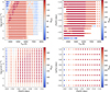 |
Fig. 1 Stellar atmospheric parameters of the synthetic spectra grid. Here, Nspec represents the number of spectra at each parameter combination. |
2 Data
2.1 Synthetic spectra
This work employed the SPECTRUM v2. 77 synthesis code (Gray & Corbally 1994) to perform radiative transfer calculations on the ATLAS9 grid of stellar atmospheric models of Castelli & Kurucz (2003). We first constructed a three-dimensional grid of model atmospheres covering Teff=3500−8000 K (Δ Teff= 100 K for Teff=3500−6000 K, then 250 K steps to 8000 K), log g=0.00−5.00 dex(Δ log g=0.25 dex), and [Fe/H]=−4.0 to −1.0 dex(Δ[Fe/H]=0.2), yielding 11 763 stellar atmospheric models (see Figure 1).
In the radiation transfer phase, we independently adjusted [O/Fe] and [Mg/Fe] with values of −0.2, 0.0, 0.2, 0.4, 0.6, 0.8, 1.0, and 1.2 dex. The process is as follows.
First, the solar logarithmic abundances of O or Mg are read from stdatom.dat as  ), and the metallicity [M/H] from the stellar atmospheric model header is added to all metal elements (in this study, we set [M/H]=[Fe/H]), resulting in
![Mathematical equation: $A_{X}^{\mathrm{model}}=A_{X}^{\odot}+[\mathrm{Fe}/\mathrm{H}].$](/articles/aa/full_html/2026/02/aa56476-25/aa56476-25-eq2.png) (1)
Therefore, to achieve a non-zero [X/Fe], an additional offset must be applied to the abundance of the element before reading.
(1)
Therefore, to achieve a non-zero [X/Fe], an additional offset must be applied to the abundance of the element before reading.
Then, for each grid point (Teff, log g,[Fe/H]) and the target differential [X/Fe]target, the corresponding abundance in stdatom.dat is modified:
![Mathematical equation: $A_{X}^{\text {file }}=A_{X}^{\odot}+[X/\mathrm{Fe}]_{\text {target }}.$](/articles/aa/full_html/2026/02/aa56476-25/aa56476-25-eq3.png) (2)
After reading, SPECTRUM adds the [Fe/H] value, resulting in the final abundance:
(2)
After reading, SPECTRUM adds the [Fe/H] value, resulting in the final abundance:
![Mathematical equation: $A_{X}^{\mathrm{model}}=A_{X}^{\odot}+[\mathrm{Fe}/\mathrm{H}]+[X/\mathrm{Fe}]_{\text {target }}.$](/articles/aa/full_html/2026/02/aa56476-25/aa56476-25-eq4.png) (3)
(3)
All spectra were computed with the nita switch and without the f option. Therefore, before output, the SPECTRUM program solves the radiative transfer equation with only continuous absorption, using the same stellar atmospheric model. The resulting composite spectrum is normalized by dividing the intensity spectrum Iλ by the pure continuum spectrum Ic, λ, yielding a normalized intensity spectrum with F/Fc=1. If the f switch is used, absolute flux is output instead. The distinction between the default “normalized-intensity spectrum” mechanism and the f switch is detailed in the document (Gray & Corbally 1994). For further explanation of the physical background and observational normalization techniques, see Gray (2021).
Additionally, we assigned microturbulent velocities vturb based on (Teff, log g,[Fe/H]) in the following segments (García Pérez et al. 2016; Holtzman et al. 2018): For log g ≥ 3.5 dex and Teff ≥ 5000 K,
 (4)
for log g ≥ 3.5 dex and Teff<5000 K,
(4)
for log g ≥ 3.5 dex and Teff<5000 K,
 (5)
for log g<3.5 dex and [Fe/H] ≥−1,
(5)
for log g<3.5 dex and [Fe/H] ≥−1,
 (6)
for log g<3.5 dex and [Fe/H]<−1,
(6)
for log g<3.5 dex and [Fe/H]<−1,
 (7)
(7)
The initial resolution of the synthetic spectra is 0.02 Å, covering a wavelength range from 2550 to 10 000 Å. Each stellar atmospheric model corresponds to 16 different values of [O/Fe] and [Mg/Fe], totaling approximately 11 763 × 16 ≈ 1.88 × 10⁵ spectra for subsequent regression analysis.
2.2 Low-resolution processing
As described in Section 1, CSST operates with a low spectral resolution of approximately R ≈ 200. Its wide field of view (∼1.1 deg2) and high limiting magnitude allow it to survey high Galactic latitude regions, thus identifying a large sample of MP stars together with crucial UV spectra. To evaluate the impact of including the UV band data on regression models for MP stars [O/Fe] and [Mg/Fe], this study quantifies the performance improvement enabled by UV spectra coverage and investigates the underlying spectroscopic reasons. To this end, we simulate low-resolution spectra as observed by CSST to provide data more closely resembling real observations, thereby supporting the development of deep learning algorithms. These algorithms are specifically designed to predict [O/Fe] and [Mg/Fe] from spectra that include UV spectra coverage under low resolution (R ≈ 200), which is introduced in detail in Section 3.
The core idea of the resolution degradation process is to use a convolution based method to blur the fine structures in the original high resolution spectra to match the target resolution. In this process, we construct the output wavelength grid {Λj} using a constant resolution R ≡ Λ/Δ Λ. Starting from Λ0=λmin, the grid is constructed recursively as
 (8)
until ΛN−1 ≤λmax. Each wavelength point has an effective width of
(8)
until ΛN−1 ≤λmax. Each wavelength point has an effective width of  to maintain constant resolution over the entire wavelength range.
For each target wavelength Λj, we performed a local Gaussian convolution on the trimmed high resolution spectrum {λi, Fi} to mimic the point spread function (PSF) of the spectrograph. The full width at half maximum (FWHM) of the Gaussian kernel is given by
 (9)
and the kernel is normalized to unit area as
(9)
and the kernel is normalized to unit area as
![Mathematical equation: $G_{j}(\lambda)=\frac{1}{\sigma_{j} \sqrt{2 \pi}} \exp \left[-\frac{\left(\lambda-\Lambda_{j}\right)^{2}}{2 \sigma_{j}^{2}}\right],$](/articles/aa/full_html/2026/02/aa56476-25/aa56476-25-eq12.png) (10)
where
(10)
where  .
.
The downsampled spectral flux at each Λj is computed by
 (11)
To accelerate the processing of nearly 1.9 × 10⁵ spectra, Python multiprocess.Pool was employed for parallel computation. For each target wavelength {Λj}, we first prepared extended subarrays {λi, Fi}, then distributed the convolution tasks across multiple CPU cores, and finally collected the downsampled spectra {Λj, F̃}. To reduce the computational load, the convolution range was truncated to ± 5 FWHM, which significantly cuts down computation time. In practice, continuous integration is replaced by discrete summation over the clipped original wavelength grid. The convolution for each Λj point was computed using the kernel function (e.g., Gaussian function), and normalized by dividing by the total kernel weight.
(11)
To accelerate the processing of nearly 1.9 × 10⁵ spectra, Python multiprocess.Pool was employed for parallel computation. For each target wavelength {Λj}, we first prepared extended subarrays {λi, Fi}, then distributed the convolution tasks across multiple CPU cores, and finally collected the downsampled spectra {Λj, F̃}. To reduce the computational load, the convolution range was truncated to ± 5 FWHM, which significantly cuts down computation time. In practice, continuous integration is replaced by discrete summation over the clipped original wavelength grid. The convolution for each Λj point was computed using the kernel function (e.g., Gaussian function), and normalized by dividing by the total kernel weight.
Figure 2 presents a comparison between the original high resolution spectra and the degraded low-resolution version. The distinction between the two spectra is evident, highlighting the effect of resolution degradation on spectral features.
2.3 Spectral analysis in different parameter spaces
Before quantitatively estimating the experiments, we first performed a qualitative analysis of the simulated CSST low-resolution spectra in the UV band, investigating the spectral features under different [O/Fe] and [Mg/Fe] abundance conditions to assess the potential contribution of the UV band to abundance estimation. Overall, the UV band data exhibited significant spectral line features in all of parameter spaces.
Figure 3 shows the variation of the OH molecular band and Mg lines in the UV band at different Teff. The depth of the OH molecular band initially increases and then decreases with rising Teff, with the peak occurring around K-type stars (approximately 4000−5000 K). At low Teff (around 3500 K, M-type stars), OH molecules are abundant, but the UV radiation is weak, causing the spectral lines to be inconspicuous. At intermediate Teff (around 4000−5000 K, from K-type to early G-type stars), UV radiation increases, and OH molecules still remain abundant, leading to a peak in line strength. At high Teff(>5500 K, from G-type to F- and A-type stars), the temperature rise causes OH molecules to dissociate extensively, weakening the spectral lines. By late F-type and A-type stars (approximately 7000-8000 K), the OH molecular band virtually disappears.
Similarly, the depth of the Mg I line first increases and then decreases with increasing Teff, with the peak occurring around K-type to G-type stars (approximately 4000−5800 K). At low Teff (around 3500 K, M-type stars), magnesium predominantly exists in its neutral Mg I form. At intermediate Teff (approximately 4000−5800 K, from K-type to G-type stars), as the Teff increases, the excitation effect dominates, enhancing the line strength; however, the ionization effect begins to emerge. At high Teff (>6000 K, from F-type to A-type stars), the ionization effect becomes dominant, reducing the amount of neutral Mg I, causing the line strength to decrease. By 8000 K in A-type stars, the Mg I line becomes extremely weak. Similarly, the Mg II line strength also follows a trend of first increasing and then decreasing with rising Teff.
Figure 4 shows the effect of different log g on the OH molecular band and Mg absorption lines in the UV band. As the log g increases, the depth of the OH molecular band becomes deeper and stronger. An increase in log g results in higher atmospheric pressure, which promotes the formation of OH molecules, thereby enhancing the strength of the OH absorption band in the UV band.
At the same time, the intensity of the Mg I line increases with increasing log g, while the Mg II line weakens. This is because, as log g increases, the higher atmospheric pressure leads to a more significant recombination of Mg II to Mg I, resulting in a decrease in Mg II and an increase in Mg I. Therefore, for stars with similar Teff, the Mg I lines of dwarf stars (high log g) are typically stronger than those of giant stars (low log g), while the Mg II lines of giant stars are typically stronger than those of dwarf stars.
Figure 5 illustrates the impact of [Fe/H] on key UV spectral features. It is important to note that the variations observed in the OH and Mg lines as a function of [Fe/H] arise from the design of the synthetic spectra. Specifically, the absolute elemental abundances are coupled through the standard relation, [Mg/H]=[Mg/Fe]+[Fe/H], where [Mg/Fe] better reflects the established empirical trends of Galactic chemical evolution (GCE).
As depicted in the figure, with decreasing [Fe/H], the strengths of OH molecular band, the Mg II doublet, and the Mg I line progressively increase, with the enhancement of the Mg II doublet being the most significant. For metallicities where [Fe/H]<−2.8, the strength of the Mg II doublet surpasses that of the Mg I line. As [Fe/H] decreases further, the difference in strength between these two features is amplified.
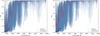 |
Fig. 2 Comparison between the original high resolution spectra (blue) and the low-resolution spectra (red) degraded to R ≈ 200 through Gaussian convolution. Both panels cover the 2550−10 000 Å range, with the left panel showing an MP star with [O/Fe]=0.4, [Mg/Fe]=0.0, Teff=4700 K, log g=5.0, and [Fe/H]=−2.0, and the right panel showing an MP star with [O/Fe]=0.0, [Mg/Fe]=0.4, and the same other parameters. |
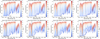 |
Fig. 3 Variation of UV spectral flux as a function of Teff with fixed parameters (log g=3.0,[Fe/H]=−1.0). Upper row: variation for the [O/Fe] ratio of −0.2,+0.2,+0.6, and +0.8. Lower row: same as the upper row but for [Mg/Fe] ratios. The depth of the OH molecular band first increases and then decreases with rising Teff, with the peak occurring around K-type stars (approximately 4000−5000 K). Similarly, the depth of the Mg I line increases and then decreases with rising Teff, with the peak occurring around K-type to G-type stars (approximately 4000−5800 K), while the Mg II line continuously strengthens with increasing Teff. |
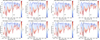 |
Fig. 4 Similar to Figure 3, but showing the variation of UV spectral flux as a function of log g. The synthetic spectra were calculated for fixed parameters (Teff=4500 K,[Fe/H]=−1.0). Upper row: variation for the [O/Fe] ratios of −0.2,+0.2,+0.6, and +0.8. Lower row: same as the upper row but for [Mg/Fe] ratios. As the log g increases, the depth of the OH molecular band becomes deeper. The intensity of the Mg I line increases with increasing log g, while the Mg II line weakens. |
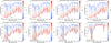 |
Fig. 5 Similar to Figures 3 and 4, but showing the variation of UV spectral flux as a function of [Fe/H]. The synthetic spectra were calculated for fixed parameters (Teff=4500 K, log g=3.0). Upper row: variation for the [O/Fe] ratios of +0.2,+0.4,+0.8, and +1.2. Lower row: same as the upper row but for [Mg/Fe] ratios. As [Fe/H] decreases, the strength of the OH molecular band, Mg II doublet, and Mg I line gradually increases, with the Mg II doublet showing a more significant increase. When [Fe/H]<−2.8, the strength of the Mg II doublet surpasses that of the Mg I line, and as [Fe/H] decreases further, the strength difference between the two increases. |
3 Methods
3.1 Preliminary
Self-attention, a cornerstone of the Transformer architecture (Vaswani et al. 2017), is a mechanism that allows a model to weigh the importance of different elements in an input sequence when processing a specific element. It enables the model to capture long range dependencies and contextual relationships within the sequence itself.
Let the input sequence be represented by a matrix X ∈ ℝn × dmodel, where n is the sequence length and dmodel is the dimension of the embedding for each token. From this input, we derive three distinct matrices: the query (Q), key (K), and value (V) matrices. These are produced by multiplying the input matrix X with three separate, learnable weight matrices WQ ∈ ℝdmodel × dk, WK ∈ ℝdmodel × dk, and WV ∈ ℝdmodel × dv: Q=XWQ; K = XWK; V = XWV. Here, dk is the dimension of the keys and queries, and dv is the dimension of the values.
The core of the self-attention mechanism is the Scaled Dot-Product Attention function. The output is computed as a weighted sum of the values, where the weight assigned to each value is determined by the dot-product similarity of the query with its corresponding key. The formula is as follows:
 (12)
In this equation, the term QK⊤ calculates the dot product between every query vector in Q and every key vector in K, resulting in a matrix of attention scores that reflects the similarity between each pair of positions in the sequence. To prevent the dot products from growing excessively large and pushing the softmax function into regions with vanishing gradients, the scores are scaled by a factor of
(12)
In this equation, the term QK⊤ calculates the dot product between every query vector in Q and every key vector in K, resulting in a matrix of attention scores that reflects the similarity between each pair of positions in the sequence. To prevent the dot products from growing excessively large and pushing the softmax function into regions with vanishing gradients, the scores are scaled by a factor of  . The softmax function is then applied to normalize the scaled scores into a probability distribution, yielding the attention weights. Finally, this matrix of attention weights is multiplied by the Value matrix V to produce the output of the self-attention layer. This output provides a new representation for each token that is a weighted average of all token values in the sequence, thereby encoding rich contextual information.
3.2 GloCal-Attention
To address the issue of scattered attention in traditional self-attention mechanisms, Zhang et al. (2024c) proposed an attention-enhanced operator and constructs the spectral transformer (SPT) model based on it. The SPT model was designed to estimate the age and mass of red giant stars from their spectra. Its core innovation is the multi-head Hadamard Self-Attention (multi-head HSA) mechanism. Unlike conventional self-attention that relies on dot-product similarity, the HSA operator computes attention scores using the Hadamard product (i.e., element-wise multiplication) between normalized Query and Key matrices. This is combined with an enhanced_softmax function to create a sharper and more focused attention distribution, better suited for continuous spectral data. However, as the sequence length increases, self-attention can still suffer from the problem of scattered attention. A typical example in transformers is the degradation of their performance and an increased tendency for hallucination as the input context length grows in large language models.
It can be fundamentally attributed to the mathematical properties of the self-attention mechanism, the core component of the Transformer architecture. The primary bottlenecks arise from attention score dilution. A critical vulnerability emerges from the interplay between the QK⊤ operation and the subsequent softmax normalization, especially as the sequence length, n, grows. The softmax function transforms the raw attention scores into a probability distribution, forcing the sum of weights across all n tokens to equal one. As n becomes exceedingly large (e.g., hundreds of thousands of tokens), the denominator of the softmax function,  , inflates due to the sheer volume of tokens. This leads to a phenomenon known as attention dilution. The weights assigned to a few genuinely critical tokens are suppressed, as the finite probability mass is distributed across a vast number of irrelevant or noisy tokens. The cumulative effect of these numerous, albeit individually small, weights on their corresponding Value vectors (V) can introduce significant noise that overwhelms the signal from a few pertinent tokens. This loss of focus prevents the model from concentrating its computational resources on the most relevant parts of the context, thereby increasing the likelihood of generating outputs that are unfaithful to the source material.
Therefore, to alleviate the issue of scattered attention in self-attention mechanisms under long-sequence spectra, we propose a self-attention method called SPT-GloCal, which combines a score-aware backbone attention with global attention. This approach aims to help self-attention better focus on the phenomenon of “perceptual isolation” caused by long sequences, where the attention scores across the sequence tend to approach zero more easily.
Score-aware information flow. In the context of long sequence data processing, the conventional softmax function, by its nature of normalizing scores into a probability distribution that sums to unity, can inadvertently dilute the influence of highly relevant features. The fixed total probability mass must be distributed across all elements in the sequence, which can lead to significant information being obscured by a long tail of low weight, noisy elements. To address this limitation, we introduce a score-aware information flow mechanism. This methodology is engineered to iteratively prune insignificant candidate items and re-emphasize the most salient information, thereby refining the information flow within the attention computation. The general algorithmic procedure is depicted in Figure 6.
First, we defined the model’s hyperparameters: the number of window layers n, the input sequence length l, and the number of competitive filtering layers p. The function Ψ refers to the enhanced softmax as detailed in the work by Zhang et al. (2024 c). Within the i-th sliding window and at the r-th competitive layer, we have:
 (13)
In this equation, Qi ∈ ℝnu × d* and Ki ∈ ℝnw × d* are the query and key matrices within the i-th window of length nw. The operator ○ denotes the Hadamard product (i.e., element-wise multiplication), and d* is the feature dimension of the query and key vectors at this competitive layer.
(13)
In this equation, Qi ∈ ℝnu × d* and Ki ∈ ℝnw × d* are the query and key matrices within the i-th window of length nw. The operator ○ denotes the Hadamard product (i.e., element-wise multiplication), and d* is the feature dimension of the query and key vectors at this competitive layer.
For each window, we select the top-n elements that satisfy a cumulative score contribution threshold α to proceed to the next competitive layer. The set of indices Iir is identified, and the scores for the subsequent layer are composed exclusively of the elements corresponding to these indices. This is formally expressed as:
![Mathematical equation: $\mathbf{I}_{\text {ir }}=\left\{j \mid \sum \operatorname{rank}\left(\operatorname{Score}\left(Q_{i}, K_{i}\right)_{r}\right)[j]<\alpha\right\}$](/articles/aa/full_html/2026/02/aa56476-25/aa56476-25-eq19.png) (14)
(14)
![Mathematical equation: $\operatorname{Score}\left(Q_{i}, K_{i}\right)_{r+1}=\left\{\left(\operatorname{Score}\left(Q_{i}, K_{i}\right)_{r}\right)[j] \mid j \in \mathbf{I}_{\mathbf{i r}}\right\}.$](/articles/aa/full_html/2026/02/aa56476-25/aa56476-25-eq20.png) (15)
(15)
Finally, the competitive process terminates when the number of candidate elements falls below a threshold γ. The output of the Score-aware information flow can then be represented as:
 (16)
where Vp denotes the value vectors corresponding to the attention scores retained in the final layer. In essence, the proposed procedure decouples the competitive selection mechanism of the softmax function from its inherent normalization constraint. This is achieved by first acquiring principal information from local regions through a layer wise competitive filtering process, followed by a final normalization step.
(16)
where Vp denotes the value vectors corresponding to the attention scores retained in the final layer. In essence, the proposed procedure decouples the competitive selection mechanism of the softmax function from its inherent normalization constraint. This is achieved by first acquiring principal information from local regions through a layer wise competitive filtering process, followed by a final normalization step.
Overall information flow. To integrate the global context with the salient local information derived from our proposed mechanism, the final output is formulated as a weighted combination:
 (17)
where the component set is C={original, flow}. The term gc ∈ [0, 1] is a learnable gating parameter that adaptively balances the contribution from the original attention output (Ooriginal) and the score-aware flow output (Oflow).
(17)
where the component set is C={original, flow}. The term gc ∈ [0, 1] is a learnable gating parameter that adaptively balances the contribution from the original attention output (Ooriginal) and the score-aware flow output (Oflow).
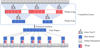 |
Fig. 6 Model framework. It employs a multi-round competitive selection mechanism. The process begins with input tokens (gray squares). In long sequences, the standard softmax function introduces a competition that can diminish the informational contribution of many tokens to near zero. To counteract this and decouple the selection process (“competition”) from the intrinsic value of the information, our model iteratively identifies and discards less salient features through multiple rounds. The “winner” tokens from each round are highlighted within the boxes outlined with blue dashes. The final set of “Winner” tokens, representing the most critical local information, is then integrated with the initial sequence to enrich the model’s overall perceptual field. |
3.3 Training details
To train and evaluate our SPT-GloCal model, we first randomly partitioned the full dataset of approximately 188 000 synthetic spectra into a training set (80%), a validation set (10%), and an independent test set (10%). The model is designed to take a low-resolution spectrum as input and regress the [O/Fe] and [Mg/Fe] abundance ratios.
The model architecture is based on the Vision Transformer (ViT), with the standard self-attention mechanism replaced by our proposed GloCal-Attention. The overall configuration adopts an embedding dimension of 768, 12 transformer blocks, and 12 attention heads per block, resulting in approximately 85.2 million trainable parameters. For model training, we adopted the following strategies:
Optimization. We employed the Adam optimizer for the training process. Its parameter settings were fixed at β1=0.9, β2=0.999, and ε=10−8 to ensure stable and efficient convergence.
Learning rate policy. An initial learning rate of 10−4 was used. To refine convergence in later stages, we applied a decay strategy, reducing the learning rate by a factor of 0.8 every 100 epochs.
Regularization. To mitigate overfitting, L2 regularization with a weight decay coefficient of 5 × 10⁻⁴ was applied. This encourages the model to learn smoother and more generalizable weight distributions.
Weight initialization. All model weights were initialized using a truncated normal distribution. This strategy was chosen to facilitate a stable starting point for the optimization.
Early stopping. An early stopping mechanism was implemented to prevent overfitting and save computational resources. If the model’s performance on the validation set did not show improvement over ten consecutive epochs, the training was terminated. The final model parameters were taken as the average of the weights from these last ten epochs to enhance robustness.
To investigate the impact of the UV data, two separate models were trained with identical configurations: one using the full spectral range (2550−10 000 Å) and another using only the optical range (4000–10 000 Å).
3.4 Evaluation metrics
To quantitatively assess the predictive accuracy of our models, we used two standard statistical metrics: the mean absolute error (MAE) and the standard deviation of the residuals (σ). All performance evaluations were conducted on the independent test set. The metrics are defined as follows:
 (18)
(18)
 (19)
where N is the total number of samples in the test set, yi is the true abundance ratio for the i-th sample, ŷi is the corresponding model prediction, and r̄ is the mean of all residuals (yi−ŷi).
(19)
where N is the total number of samples in the test set, yi is the true abundance ratio for the i-th sample, ŷi is the corresponding model prediction, and r̄ is the mean of all residuals (yi−ŷi).
Statistical comparison of prediction errors for [O/Fe] and [Mg/Fe] over the 2550−10 000 Å and 4000−10 000 Å spectral ranges.
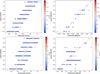 |
Fig. 7 Predicted versus true [O/Fe] (left) and [Mg/Fe] (right) on the test set. Upper row: model trained on 2550−10 000 Å spectra. Lower row: model trained on 4000–10 000 Å spectra. Colors encode the local point density; the dashed line marks the 1:1 relation. |
4 Results
4.1 Global regression performance of SPT-GloCal
We evaluated the performance of the SPT-GloCal model on the independent test set using the metrics defined in Section 3.4. Table 1 summarizes the prediction accuracy achieved by SPT-GloCal when the UV band (2550−4000 Å) is included or removed from the input spectra. For [O/Fe] the standard deviation of the residuals decreases from σ=0.135 to σ=0.063, and the MAE is halved, from 0.078 to 0.037. The effect is even more striking for [Mg/Fe]: the error scatter shrinks by almost an order of magnitude (from σ=0.054 to σ=0.0068) and the MAE drops from 0.010 to only 6.5 × 10⁻⁴.
Figure 7 shows the regression results for [O/Fe] and [Mg/Fe]. The upper row present the full band model (2550−10 000 Å), where the majority of the predicted values for both [O/Fe] and [Mg/Fe] closely follow the 1:1 relation. The lower row, based on a model trained only with the optical band (4000–10 000 Å), show systematic deviations in the predictions for [O/Fe] across all abundances, while [Mg/Fe] exhibits a broader tail at low abundances. These results highlight that, although the classical indicators for oxygen and magnesium are primarily found in the optical band, the diagnostic information provided by the UV range is crucial for improving prediction accuracy.
4.2 Error analysis in different parameter spaces
In different physical parameter spaces, we analyzed the predictive performance of [O/Fe] and [Mg/Fe]. As shown in Figures 8 and 9, the data that included the UV band demonstrated a better predictive performance for [O/Fe] and [Mg/Fe] in terms of Teff, log g,[Fe/H], and elemental distribution compared to the data without the UV band, with smaller corresponding mean squared error (MSE) and σ. Moreover, the prediction uncertainties in the data with UV band exhibited relatively smaller fluctuations, resulting in more stable predictions that were less affected by atmospheric parameters.
In detail, Figure 8 shows that the improvement in the UV band is most pronounced in the 4500−6000 K range, with the difference being significantly higher than in other temperature ranges. This indicates that the UV band spectra effectively reduces the estimation errors of [O/Fe] at these temperatures. For log g, the MSE and σ values for the non-UV band data increase significantly with higher log g, while the MSE and σ of the [O/Fe] estimates with the UV band data show a slight decreasing trend and smaller fluctuations. From the difference in the error curves, it is evident that the impact of the UV band spectra on improving the estimation accuracy of [O/Fe] becomes more significant as log g increases (with the difference between the curves increasing). Similarly, for [Fe/H], as its value decreases, the estimation errors of [O/Fe] without the UV band spectra increase monotonically in terms of MSE and σ. This result supports the general finding in the literature that [O/Fe] estimations for MP stars are typically challenging and subject to significant uncertainties, particularly when relying solely on standard optical diagnostics (e.g., Zhao et al. 2016; Amarsi et al. 2019). However, the introduction of the UV band spectra leads to a reduction in both MSE and σ, which provides new confidence for future estimates of [O/Fe] for MP stars and highlights the important role in the UV band plays in this process. Additionally, we observe that as the value of [O/Fe] increases, the estimation accuracy improves, which is consistent with the trend that the estimation accuracy of [O/Fe] increases as [Fe/H] decreases, since lower [Fe/H] generally correlates with higher abundance of α-elements.
In Figure 9, for Teff, the improvement with the UV band data is more noticeable in the 3500−5300 K and 6300−8000 K ranges, indicating that the UV band spectra is more effective at reducing the estimation errors of [Mg/Fe] in these temperature ranges. In comparison, the UV band data improves the [Mg/Fe] estimation accuracy less than [O/Fe], which is expected in our study. This is because, for [Mg/Fe], the estimation is already better with or without the UV band spectra than for [O/Fe], and thus the potential for further improvement is smaller. For log g, similar to [O/Fe], the MSE and σ for the data without the UV band increase with increasing log g, while the [Mg/Fe] estimates with the UV band data show smaller fluctuations. The difference in error curves indicates that the effect of the UV band spectra on improving [Mg/Fe] estimation accuracy becomes more significant as log g increases. For [Fe/H], as its value decreases, the MSE and σ curves for the data with the UV band exhibit smaller fluctuations, with only a small difference compared to the nonUV data. For the errors in the distribution of [Mg/Fe] values, the non-UV data show larger fluctuations and a bimodal pattern, while the errors with the UV band data are much smaller, indicating a more stable prediction.
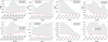 |
Fig. 8 Mean squared error (left) and σ (right) of the [O/Fe] prediction error across the four-dimensional parameter space (Teff, log g,[Fe/H], [O/Fe]). Red solid line: including the UV band data (2550−10 000 Å); blue dashed line: optical only (4000−10 000 Å). |
Performance of SPT-GloCal versus tree boosting baselines in estimating [O/Fe] and [Mg/Fe] over the 2550−10 000 Å spectral ranges.
Comparison of abundance determination performance for [Mg/Fe] and [O/Fe] across different methods and signal-to-noise ratios (S/N).
4.3 Model comparison
We compared the performance of the SPT-GloCal model with the SPT model proposed by Zhang et al. (2024c), which is designed to process low-resolution spectral data with UV band to predict [Fe/H] and [α/Fe], as well as several benchmark models based on tree boosting (XGBoost, LightGBM, and CatBoost) for predicting the [O/Fe] and [Mg/Fe] ratios of MP stars.
Table 2 presents the performance of different models in estimating the [O/Fe] and [Mg/Fe] abundance ratios over the spectral range of 2550−10 000 Å. The best results are highlighted in the table. As shown, SPT-GloCal outperformed the other models in terms of prediction accuracy for both [O/Fe] and [Mg/Fe]. Specifically, SPT-GloCal achieves a σ of 0.0629 and a MAE of 0.0367 for [O/Fe], outperforming XGBoost (σ=0.1262, MAE = 0.0615), LightGBM (σ=0.1358, MAE =0.0640), and CatBoost (σ=0.1269, MAE =0.0617). Similarly, for [Mg/Fe], SPT-GloCal also performs exceptionally well, with a σ of 0.0068 and an MAE of 0.0006, surpassing the other benchmark models.
Compared to the SPT model, SPT-GloCal shows an improvement in performance. For [O/Fe], the σ of SPT is 0.0736 and the MAE is 0.0453, both higher than the 0.0629 and 0.0367 of SPT-GloCal. For [Mg/Fe], the σ of SPT is 0.0079 and the MAE is 0.0007, still higher than those of SPT-GloCal. The introduction of a global attention mechanism in SPT-GloCal enhances the ability of the SPT model to process long sequence information, particularly in low-resolution spectral data. This improvement allows the model to capture key information more effectively, leading to enhanced prediction accuracy.
4.4 Performance on noisy spectra
To assess the robustness of our model under more realistic observational conditions, we conducted an additional analysis by introducing noise to the model spectra. We generated three versions of the test set by adding Gaussian noise to simulate average signal-to-noise ratios of 30, 40, and 50 per pixel. We then evaluated the performance of SPT-GloCal and all baseline models on these noisy spectra.
The results are summarized in Table 3. As expected, the precision of all models deteriorates as the S/N decreases. For instance, for [O/Fe], the SPT-GloCal model yields predictions where the σ increases from 0.2215 at S/N=50 to 0.3526 at S/N=30. A similar trend is observed for all other methods and for [Mg/Fe] predictions.
Despite the general performance degradation, SPT-GloCal consistently outperforms all other models across all tested S/N. For [O/Fe] at a challenging S/N of 30, SPT-GloCal achieves a σ of 0.3526, which is marginally better than its predecessor SPT (σ=0.3676) and substantially superior to the tree-based models (e.g., XGBoost with σ=0.6826). For [Mg/Fe], SPT-GloCal also maintains a clear advantage, demonstrating its superior ability to extract meaningful features even from noise-contaminated, low-resolution spectra. This analysis confirms that the architectural improvements in SPT-GloCal provide a tangible advantage in noise-limited scenarios, reinforcing its potential for reliable application to real CSST survey data.
5 Conclusion
This study presents a comprehensive framework for improving the abundance estimation of [O/Fe] and [Mg/Fe] in MP stars through the integration of UV spectral information and a novel deep learning model, SPT-GloCal. Motivated by the known limitations of traditional and machine learning methods in the optical only regime, especially for MP stars, we explored the diagnostic power of UV band spectra (2550−4000 Å), which is accessible to upcoming CSST survey.
To simulate realistic low-resolution observations, we generated over 180 000 synthetic spectra using SPECTRUM v2.77, spanning a wide stellar parameter grid. These spectra were processed to match the resolution of CSST (R ≈ 200) and were used to train and evaluate our models. Our analyses revealed that the key UV absorption features including OH molecular bands and Mg II/Mg I lines provide robust diagnostic signals for [O/Fe] and [Mg/Fe], especially in parameter regimes where optical lines are weak or absent.
We introduced the SPT-GloCal model, which extends the self-attention backbone with a score-aware information flow mechanism and a global-local integration strategy. This design addresses the attention dilution problem in long sequence spectral inputs, enabling the model to better preserve and extract relevant signals from complex spectra.
Quantitative results demonstrate the superiority of our approach. The inclusion of UV data reduced the MAE of [O/Fe] predictions from 0.0785 to 0.0367, and for [Mg/Fe] from 0.0010 to 0.0006. Error analyses across Teff, log g, and [Fe/H] further confirmed that UV band spectra enhance predictive stability, especially in challenging regions such as high surface gravity or low metallicity. Compared to the baseline SPT model and tree based regressors (XGBoost, LightGBM, CatBoost), SPT-GloCal consistently achieved lower residual errors, validating the effectiveness of both its architectural design and the UV inclusive spectral input.
This work highlights the underutilized potential of the UV spectra domain in stellar spectroscopy and demonstrates that even at low resolution, UV spectral features can play a critical role in stellar chemical analysis. The SPT-GloCal framework offers a scalable and physically informed solution for abundance regression, well suited to the next generation of space based spectroscopic surveys. In future work, we plan to apply this model to real CSST and UV survey data, extend its application to other α – and iron-peak elements, and incorporate uncertainty quantification into the model outputs.
Acknowledgements
This work is supported from the Strategic Priority Research Program of Chinese Academy of Sciences, grant No. XDB1160101. This study is also supported by the Natural Science Foundation of Shandong Province under grant No. ZR2024MA063, No. ZR2022MA076, and No. ZR2022MA089, the science research grants from the China Manned Space Project with No. CMS-CSST-2021-B05 and CMS-CSST-2021-A08, and the National Natural Science Foundation of China (NSFC) under grants No. 12090044, 11873037, 11803016, and 12573109.
References
- Amarsi, A. M., Nissen, P. E., Asplund, M., Lind, K., & Barklem, P. S., 2019, A&A, 622, L4 [NASA ADS] [CrossRef] [EDP Sciences] [Google Scholar]
- Ambrosch, M., Guiglion, G., Mikolaitis, Š., et al. 2023, A&A, 672, A46 [NASA ADS] [CrossRef] [EDP Sciences] [Google Scholar]
- Arnone, E., Ryan, S. G., Argast, D., Norris, J. E., & Beers, T. C., 2005, A&A, 430, 507 [NASA ADS] [CrossRef] [EDP Sciences] [Google Scholar]
- Asa’d, R., Hernandez, S., John, J. M., et al. 2024, AJ, 167, 265 [Google Scholar]
- Asplund, M., 2005, ARA&A, 43, 481 [Google Scholar]
- Barklem, P. S., & Collet, R., 2016, A&A, 588, A96 [NASA ADS] [CrossRef] [EDP Sciences] [Google Scholar]
- Beers, T. C., & Christlieb, N., 2005, ARA&A, 43, 531 [Google Scholar]
- Bergemann, M., Collet, R., Amarsi, A. M., et al. 2017, ApJ, 847, 15 [NASA ADS] [CrossRef] [Google Scholar]
- Bond, H. E., Nelan, E. P., VandenBerg, D. A., Schaefer, G. H., & Harmer, D., 2013, ApJ, 765, L12 [NASA ADS] [CrossRef] [Google Scholar]
- Bonifacio, P., Caffau, E., François, P., & Spite, M., 2025, arXiv e-prints [arXiv:2504.06335] [Google Scholar]
- Carretta, E., Gratton, R. G., & Sneden, C., 2000, A&A, 356, 238 [Google Scholar]
- Carretta, E., Bragaglia, A., Gratton, R., & Lucatello, S., 2009, A&A, 505, 139 [NASA ADS] [CrossRef] [EDP Sciences] [Google Scholar]
- Castelli, F., & Kurucz, R. L., 2003, in IAU Symposium, 210, Modelling of Stellar Atmospheres, ed. N. Piskunov, W. W. Weiss, & D. F. Gray, A20 [NASA ADS] [Google Scholar]
- Cayrel, R., Depagne, E., Spite, M., et al. 2004, A&A, 416, 1117 [NASA ADS] [CrossRef] [EDP Sciences] [Google Scholar]
- Chen, K.-J., Whalen, D. J., Wollenberg, K. M. J., Glover, S. C. O., & Klessen, R. S., 2017, ApJ, 844, 111 [Google Scholar]
- Chiaki, G., & Tominaga, N., 2020, MNRAS, 498, 2676 [Google Scholar]
- CSST Collaboration (Gong, Y., et al.) 2025, arXiv e-prints [arXiv:2507.04618] [Google Scholar]
- Deng, L.-C., Newberg, H. J., Liu, C., et al. 2012, Res. Astron. Astrophys., 12, 735 [Google Scholar]
- Ferreira Lopes, C. E., Gutiérrez-Soto, L. A., Ferreira Alberice, V. S., et al. 2025, A&A, 693, A306 [NASA ADS] [CrossRef] [EDP Sciences] [Google Scholar]
- Frebel, A., 2010, Astron. Nachr., 331, 474 [NASA ADS] [CrossRef] [Google Scholar]
- Frebel, A., & Ji, A. P., 2023, arXiv e-prints [arXiv:2302.09188] [Google Scholar]
- Frebel, A., & Norris, J. E., 2015, ARA&A, 53, 631 [Google Scholar]
- Frebel, A., Aoki, W., Christlieb, N., et al. 2005, Nature, 434, 871 [CrossRef] [Google Scholar]
- García Pérez, A. E., Allende Prieto, C., Holtzman, J. A., et al. 2016, AJ, 151, 144 [Google Scholar]
- Gratton, R. G., Carretta, E., Matteucci, F., & Sneden, C., 2000, A&A, 358, 671 [NASA ADS] [Google Scholar]
- Gray, D. F., 2021, The Observation and Analysis of Stellar Photospheres, 4th edn. (Cambridge University Press) [Google Scholar]
- Gray, R. O., & Corbally, C. J., 1994, AJ, 107, 742 [Google Scholar]
- Guiglion, G., 2025, A&A, 699, A191 [NASA ADS] [CrossRef] [EDP Sciences] [Google Scholar]
- Hartwig, T., Ishigaki, M. N., Klessen, R. S., & Yoshida, N., 2019, MNRAS, 482, 1204 [NASA ADS] [CrossRef] [Google Scholar]
- Hernandez, S., Larsen, S., Trager, S., Groot, P., & Kaper, L., 2017, A&A, 603, A119 [NASA ADS] [CrossRef] [EDP Sciences] [Google Scholar]
- Hernandez, S., Larsen, S., Trager, S., Kaper, L., & Groot, P., 2018, MNRAS, 476, 5189 [NASA ADS] [CrossRef] [Google Scholar]
- Holtzman, J. A., Hasselquist, S., Shetrone, M., et al. 2018, AJ, 156, 125 [Google Scholar]
- Ishigaki, M. N., Chiba, M., & Aoki, W., 2012, ApJ, 753, 64 [NASA ADS] [CrossRef] [Google Scholar]
- Ishigaki, M. N., Tominaga, N., Kobayashi, C., & Nomoto, K., 2018, ApJ, 857, 46 [Google Scholar]
- Iwamoto, N., Umeda, H., Tominaga, N., Nomoto, K., & Maeda, K., 2005, Science, 309, 451 [NASA ADS] [CrossRef] [Google Scholar]
- Joggerst, C. C., & Whalen, D. J., 2011, ApJ, 728, 129 [NASA ADS] [CrossRef] [Google Scholar]
- Joggerst, C. C., Almgren, A., Bell, J., et al. 2010, ApJ, 709, 11 [NASA ADS] [CrossRef] [Google Scholar]
- Kiselman, D., 2001, New A Rev., 45, 559 [Google Scholar]
- Kobayashi, C., Umeda, H., Nomoto, K., Tominaga, N., & Ohkubo, T., 2006, ApJ, 653, 1145 [NASA ADS] [CrossRef] [Google Scholar]
- Kolborg, A. N., Martizzi, D., Ramirez-Ruiz, E., et al. 2022, ApJ, 936, L26 [Google Scholar]
- Kollmeier, J., & The SDSS-V Collaboration 2025, in American Astronomical Society Meeting Abstracts, 245, American Astronomical Society Meeting Abstracts, 159.21 [Google Scholar]
- Kollmeier, J. A., Zasowski, G., Rix, H.-W., et al. 2017, arXiv e-prints [arXiv:1711.03234] [Google Scholar]
- Krauss, L. M., & Chaboyer, B., 2003, Science, 299, 65 [Google Scholar]
- Larsen, S. S., Brodie, J. P., Wasserman, A., & Strader, J., 2018, A&A, 613, A56 [NASA ADS] [CrossRef] [EDP Sciences] [Google Scholar]
- Larsen, S. S., Eitner, P., Magg, E., et al. 2022, A&A, 660, A88 [NASA ADS] [CrossRef] [EDP Sciences] [Google Scholar]
- Li, H., Aoki, W., Matsuno, T., et al. 2022a, ApJ, 931, 147 [NASA ADS] [CrossRef] [Google Scholar]
- Li, Z., Zhao, G., Chen, Y., Liang, X., & Zhao, J., 2022b, MNRAS, 517, 4875 [NASA ADS] [CrossRef] [Google Scholar]
- Liu, X. W., Yuan, H. B., Huo, Z. Y., et al. 2014, in IAU Symposium, 298, Setting the scene for Gaia and LAMOST, eds. S. Feltzing, G. Zhao, N. A. Walton, & P. Whitelock, 310 [Google Scholar]
- Magrini, L., Randich, S., Kordopatis, G., et al. 2017, A&A, 603, A2 [NASA ADS] [CrossRef] [EDP Sciences] [Google Scholar]
- Marino, A. F., Villanova, S., Milone, A. P., et al. 2011, ApJ, 730, L16 [NASA ADS] [CrossRef] [Google Scholar]
- Mashonkina, L., 2013, A&A, 550, A28 [NASA ADS] [CrossRef] [EDP Sciences] [Google Scholar]
- Milone, A. D. C., Sansom, A. E., & Sánchez-Blázquez, P., 2011, MNRAS, 414, 1227 [NASA ADS] [CrossRef] [Google Scholar]
- Palla, M., Santos-Peral, P., Recio-Blanco, A., & Matteucci, F., 2022, A&A, 663, A125 [NASA ADS] [CrossRef] [EDP Sciences] [Google Scholar]
- Roederer, I. U., Preston, G. W., Thompson, I. B., et al. 2014, AJ, 147, 136 [Google Scholar]
- Santos-Peral, P., Sánchez-Blázquez, P., Vazdekis, A., & Palicio, P. A., 2023, A&A, 672, A166 [NASA ADS] [CrossRef] [EDP Sciences] [Google Scholar]
- Shi, J., Zhao, G., Liu, S., et al. 2025, ApJ, 983, 127 [Google Scholar]
- Sneden, C., Boesgaard, A. M., Cowan, J. J., et al. 2023, ApJ, 953, 31 [CrossRef] [Google Scholar]
- Susa, H., Hasegawa, K., & Tominaga, N., 2014, ApJ, 792, 32 [NASA ADS] [CrossRef] [Google Scholar]
- Timmes, F. X., Woosley, S. E., & Weaver, T. A., 1995, ApJS, 98, 617 [NASA ADS] [CrossRef] [Google Scholar]
- Ting, Y.-S., & Weinberg, D. H., 2022, ApJ, 927, 209 [NASA ADS] [CrossRef] [Google Scholar]
- Ting, Y.-S., Conroy, C., Rix, H.-W., & Asplund, M., 2018, ApJ, 860, 159 [NASA ADS] [CrossRef] [Google Scholar]
- Vaswani, A., Shazeer, N., Parmar, N., et al. 2017, in Advances in Neural Information Processing Systems, 30, eds. I. Guyon, U. V. Luxburg, S. Bengio, H. Wallach, R. Fergus, S. Vishwanathan, & R. Garnett (Curran Associates, Inc.) [Google Scholar]
- Welsh, L., Cooke, R., Fumagalli, M., Pettini, M., & Rudie, G. C., 2024, A&A, 691, A285 [NASA ADS] [CrossRef] [EDP Sciences] [Google Scholar]
- Wu, F., Bu, Y., Zhang, M., et al. 2023, AJ, 166, 88 [NASA ADS] [CrossRef] [Google Scholar]
- Xiang, M., Ting, Y.-S., Rix, H.-W., et al. 2019, ApJS, 245, 34 [Google Scholar]
- Xing, Q.-F., Zhao, G., Liu, Z.-W., et al. 2023, Nature, 618, 712 [NASA ADS] [CrossRef] [Google Scholar]
- Yan, H., Li, H., Wang, S., et al. 2022, The Innovation, 3, 100224 [NASA ADS] [CrossRef] [Google Scholar]
- Zhang, J., Tang, B., Chang, J., et al. 2024a, Res. Astron. Astrophys., 24, 015011 [CrossRef] [Google Scholar]
- Zhang, M., Bu, Y., Wu, F., et al. 2024b, A&A, 691, A21 [NASA ADS] [CrossRef] [EDP Sciences] [Google Scholar]
- Zhang, M., Wu, F., Bu, Y., et al. 2024c, A&A, 683, A163 [NASA ADS] [CrossRef] [EDP Sciences] [Google Scholar]
- Zhao, G., Zhao, Y.-H., Chu, Y.-Q., Jing, Y.-P., & Deng, L.-C., 2012, Res. Astron. Astrophys., 12, 723 [NASA ADS] [CrossRef] [Google Scholar]
- Zhao, G., Mashonkina, L., Yan, H. L., et al. 2016, ApJ, 833, 225 [Google Scholar]
All Tables
Statistical comparison of prediction errors for [O/Fe] and [Mg/Fe] over the 2550−10 000 Å and 4000−10 000 Å spectral ranges.
Performance of SPT-GloCal versus tree boosting baselines in estimating [O/Fe] and [Mg/Fe] over the 2550−10 000 Å spectral ranges.
Comparison of abundance determination performance for [Mg/Fe] and [O/Fe] across different methods and signal-to-noise ratios (S/N).
All Figures
|
Fig. 1 Stellar atmospheric parameters of the synthetic spectra grid. Here, Nspec represents the number of spectra at each parameter combination. |
| In the text | |
|
Fig. 2 Comparison between the original high resolution spectra (blue) and the low-resolution spectra (red) degraded to R ≈ 200 through Gaussian convolution. Both panels cover the 2550−10 000 Å range, with the left panel showing an MP star with [O/Fe]=0.4, [Mg/Fe]=0.0, Teff=4700 K, log g=5.0, and [Fe/H]=−2.0, and the right panel showing an MP star with [O/Fe]=0.0, [Mg/Fe]=0.4, and the same other parameters. |
| In the text | |
|
Fig. 3 Variation of UV spectral flux as a function of Teff with fixed parameters (log g=3.0,[Fe/H]=−1.0). Upper row: variation for the [O/Fe] ratio of −0.2,+0.2,+0.6, and +0.8. Lower row: same as the upper row but for [Mg/Fe] ratios. The depth of the OH molecular band first increases and then decreases with rising Teff, with the peak occurring around K-type stars (approximately 4000−5000 K). Similarly, the depth of the Mg I line increases and then decreases with rising Teff, with the peak occurring around K-type to G-type stars (approximately 4000−5800 K), while the Mg II line continuously strengthens with increasing Teff. |
| In the text | |
|
Fig. 4 Similar to Figure 3, but showing the variation of UV spectral flux as a function of log g. The synthetic spectra were calculated for fixed parameters (Teff=4500 K,[Fe/H]=−1.0). Upper row: variation for the [O/Fe] ratios of −0.2,+0.2,+0.6, and +0.8. Lower row: same as the upper row but for [Mg/Fe] ratios. As the log g increases, the depth of the OH molecular band becomes deeper. The intensity of the Mg I line increases with increasing log g, while the Mg II line weakens. |
| In the text | |
|
Fig. 5 Similar to Figures 3 and 4, but showing the variation of UV spectral flux as a function of [Fe/H]. The synthetic spectra were calculated for fixed parameters (Teff=4500 K, log g=3.0). Upper row: variation for the [O/Fe] ratios of +0.2,+0.4,+0.8, and +1.2. Lower row: same as the upper row but for [Mg/Fe] ratios. As [Fe/H] decreases, the strength of the OH molecular band, Mg II doublet, and Mg I line gradually increases, with the Mg II doublet showing a more significant increase. When [Fe/H]<−2.8, the strength of the Mg II doublet surpasses that of the Mg I line, and as [Fe/H] decreases further, the strength difference between the two increases. |
| In the text | |
|
Fig. 6 Model framework. It employs a multi-round competitive selection mechanism. The process begins with input tokens (gray squares). In long sequences, the standard softmax function introduces a competition that can diminish the informational contribution of many tokens to near zero. To counteract this and decouple the selection process (“competition”) from the intrinsic value of the information, our model iteratively identifies and discards less salient features through multiple rounds. The “winner” tokens from each round are highlighted within the boxes outlined with blue dashes. The final set of “Winner” tokens, representing the most critical local information, is then integrated with the initial sequence to enrich the model’s overall perceptual field. |
| In the text | |
|
Fig. 7 Predicted versus true [O/Fe] (left) and [Mg/Fe] (right) on the test set. Upper row: model trained on 2550−10 000 Å spectra. Lower row: model trained on 4000–10 000 Å spectra. Colors encode the local point density; the dashed line marks the 1:1 relation. |
| In the text | |
|
Fig. 8 Mean squared error (left) and σ (right) of the [O/Fe] prediction error across the four-dimensional parameter space (Teff, log g,[Fe/H], [O/Fe]). Red solid line: including the UV band data (2550−10 000 Å); blue dashed line: optical only (4000−10 000 Å). |
| In the text | |
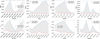 |
Fig. 9 Same as Figure 8, but showing the [Mg/Fe] prediction error. |
| In the text | |
Current usage metrics show cumulative count of Article Views (full-text article views including HTML views, PDF and ePub downloads, according to the available data) and Abstracts Views on Vision4Press platform.
Data correspond to usage on the plateform after 2015. The current usage metrics is available 48-96 hours after online publication and is updated daily on week days.
Initial download of the metrics may take a while.