| Issue |
A&A
Volume 706, February 2026
|
|
|---|---|---|
| Article Number | A153 | |
| Number of page(s) | 14 | |
| Section | The Sun and the Heliosphere | |
| DOI | https://doi.org/10.1051/0004-6361/202556711 | |
| Published online | 06 February 2026 | |
Evolution of Alfvénic slow wind parcels coming from the same solar source: observations by Parker Solar Probe, Solar Orbiter, and Wind
1
Institute for National Astrophysics, Institute for Space Astrophysics and Planetology, Via del Fosso del Cavaliere, 100 00133 Rome Italy
2
Istituto per la Scienza e la Tecnologia dei Plasmi, Consiglio Nazionale delle Ricerche Via Amendola 122/D 70126 Bari, Italy
3
Space and Plasma Physics, School of Electrical Engineering and Computer Science, KTH Royal Institute of Technology Teknikringen 31 114 28 Stockholm, Sweden
4
Advanced Heliophysics Inc, Pasadena CA 91106, USA
5
ASI – Italian Space Agency, Via del Politecnico snc 00133 Roma, Italy
6
Space Sciences Laboratory, University of California Berkeley CA 94720, USA
7
Earth, Planetary, and Space Sciences, University of California Los Angeles CA 90095, USA
8
National Institute for Astrophysics, Astrophysical Observatory of Torino Via Osservatorio 20 10025 Pino Torinese, Italy
9
Planetek Italia S.R.L., Via Massaua 12 70132 Bari BA, Italy
10
LEONARDO SpA Grottaglie 74023 Taranto, Italy
11
TSD-Space Via San Donato 23 80126 Napoli, Italy
12
University College London, Mullard Space Science Laboratory, Holmbury St. Mary Dorking Surrey RH5 6NT, UK
13
Institut de Recherche en Astrophysique et Planétologie, CNRS, Université de Toulouse CNES Toulouse, France
14
Southwest Research Institute 6220 Culebra Road San Antonio TX 78238, USA
★ Corresponding author: This email address is being protected from spambots. You need JavaScript enabled to view it.
Received:
1
August
2025
Accepted:
24
November
2025
Abstract
Context. At the end of April 2021, Parker Solar Probe (PSP) was in alignment with Solar Orbiter and one week later with Earth, observing solar wind streams originating from the same region of the Sun. During the first conjunction, PSP was at 0.10 au and Solar Orbiter at 0.89 au while, during the second conjunction with Earth, PSP was at 0.33 au.
Aims. During the two conjunctions, PSP, Solar Orbiter and Earth were connected to the same solar source, an open field region in the neighborhood of a pseudostreamer configuration that is a typical source of Alfvénic slow wind streams. This particular orbital configuration allows us to study not only the evolution of Alfvénic turbulence in the slow wind using multi-s/c measurements at different heliocentric distances, but also the magnetic evolution of the solar source region.
Methods. In this work, we reconstructed the solar source using a potential field source surface model and performed a spectral analysis by using magnetic field observations and plasma parameters from spacecraft located at different heliocentric distances to characterize solar wind fluctuations. We then investigated the radial evolution of the turbulent energy transfer rate through the Politano-Pouquet law.
Results. The open field region identified as the solar source of the different plasma parcels is characterized by a well-developed pseudostreamer configuration with strong non-monotonic expansion of the open magnetic field that gradually decayed one week later. In turn, in situ observations, although showing a general radial evolution of Alfvénicity due to solar wind expansion, may also reflect the changes experienced by the solar source. The radial weakening of the v-b alignment and the predominance of magnetic energy are associated with an increase in the intermittency of the fluctuations at MHD scales, providing insight on the interaction between Alfvénic fluctuations and turbulence in the heliosphere. The energy transfer rate shows a rapid decay as a function of the radial distance, indicating possible fast energy dissipation for the sample analyzed in this work.
Conclusions. Results show a strong radial dependence of Alfvénicity, energy equipartition, homogeneities of the fluctuations and turbulent energy transfer, highlighting how both the solar source evolution and the interaction with local inhomogeneities can shape the properties of solar wind turbulence in different points of the heliosphere.
Key words: turbulence / methods: data analysis / solar wind
© The Authors 2026
 Open Access article, published by EDP Sciences, under the terms of the Creative Commons Attribution License (https://creativecommons.org/licenses/by/4.0), which permits unrestricted use, distribution, and reproduction in any medium, provided the original work is properly cited.
This article is published in open access under the Subscribe to Open model. This email address is being protected from spambots. You need JavaScript enabled to view it. to support open access publication.
1. Introduction
The solar wind plasma is pervaded by large amplitude magnetic field and velocity fluctuations displaying a turbulent behavior (Bruno & Carbone 2013). Understanding the fundamental processes governing the origin and evolution of solar wind turbulence is crucial for understanding fundamental phenomena like solar wind heating, acceleration, and energetic particle transport in heliospheric and astrophysical plasmas. Indeed, plasma turbulence is pervasive throughout the universe, occurring in various settings such as stellar winds, black hole accretion disks, interstellar media, and terrestrial laboratory environments (e.g., Matthaeus & Velli 2011; Brandenburg & Nordlund 2011; Brandenburg & Lazarian 2013; Chen 2016; Beresnyak & Lazarian 2019). In this context, the solar wind offers a unique opportunity for studying plasma turbulence due to its accessibility by interplanetary probes. For this reason, the space science community has made significant efforts to investigate the characteristics and evolution of interplanetary magnetic field and solar wind velocity turbulent fluctuations. These fluctuations are strongly anisotropic, due to the presence of large scale magnetic fields, and exhibit power spectral densities that behave as power laws over a vast range of scales, with slopes that resemble predictions by Kolmogorov for fluids and Kraichnan for plasmas (Kolmogorov 1941; Iroshnikov 1963; Kraichnan 1965; Frisch 1995; Tu & Marsch 1995; Bruno & Carbone 2013; Tsurutani & Lakhina 2018).
The present picture of the radial evolution of solar wind turbulence (Bavassano et al. 1981, 1982a,b; Bruno et al. 2003; He et al. 2013; Bruno et al. 2014) in the inner heliosphere has mainly been derived from observations of high-speed streams at different heliocentric distances during a few consecutive solar rotations gathered by Helios (Schwenn & Marsch 1990). Reprocessed particle data from the Helios satellites between 0.3 and 1 au have been recently used to study the large-scale radial evolution of fast solar wind and its heating (Perrone et al. 2019a,b). The launch of Parker Solar Probe (PSP; Fox et al. 2016) and Solar Orbiter (Müller et al. 2020) has opened a new era in the investigation of the evolution of solar wind in the inner heliosphere, also exploring for the first time the solar environment as close as a few solar radii.
Solar wind streams with similar mean flow speed, observed by the same or different spacecraft at different heliocentric distances, can be used to gain a statistical overview of the behavior of solar wind turbulence in the inner heliosphere (see, e.g., Marsch & Tu 1996; Chen et al. 2020). However, it is possible to study the radial evolution of solar wind turbulence taking advantage of coordinated and synergistic measurements between several probes which cover the heliosphere up to Earth’s orbit during particular orbital configurations. For instance, differential radial alignments between spacecraft can be used to study the evolution of the same plasma parcel at different heliocentric distances, provided the travel time of the plasma is estimated correctly (e.g., Telloni et al. 2021).
Schwartz & Marsch (1983) reported the first radial alignment between the two Helios probes located at about 0.51 and 0.72 au, respectively. Although not focusing on the evolution of turbulence, these authors showed that particle adiabatic invariants are not conserved in fast wind, thus suggesting some ion perpendicular heating. Bruno & Trenchi (2014), Bruno et al. (2014), Telloni et al. (2015) investigated solar wind turbulence in the inner heliosphere exploiting alignments between MESSENGER and Wind, while Bruno & Trenchi (2014) and D’Amicis et al. (2010) studied the radial evolution of the same stream between L1 observatories and Ulysses at 1.4 au when the spacecraft was close to the ecliptic plane. More recently, Telloni et al. (2021) reported the first alignment between PSP (0.1 au) and Solar Orbiter (1 au) occurred in September 2020, and investigated the evolution of the magnetic field, finding a clear evolution from a highly Alfvénic solar wind parcel at 0.1 au, to a fully developed turbulence at 1 au. A similar scenario was found in Alberti et al. (2022) where spectral slopes and scaling laws of magnetic field fluctuations were analyzed by exploiting a radial alignment between PSP (orbiting near 0.17 au) and BepiColombo (orbiting near 0.6 au).
Another approach for studying the radial evolution of solar wind turbulence is to use streams coming from the same solar source and observed by different spacecraft at different heliocentric distances. In this context, Perrone et al. (2022) studied in detail the radial evolution of a homogeneous recurrent fast stream coming from the same solar source from 0.1 au to Earth. By means of combined observations by Solar Orbiter, which observed the stream close to Earth in two consecutive solar rotations, and PSP, which was connected to the same coronal hole during its sixth solar encounter, they investigated both large- and small-scale properties of turbulence within this recurrent stream. The authors also investigated the nature of the turbulent magnetic fluctuations around around proton scales in terms of their statistical association with the presence of coherent structures close to Sun and Earth in the expanding solar wind.
Until a few years ago, the study of the radial evolution of the solar wind turbulence were mainly focused on fast streams, since the slow wind evolution with heliocentric distance was observed to be comparatively weaker (e.g., Bruno et al. 2003; Bruno & Carbone 2013). Indeed, within the dichotomy between fast and slow wind, the latter is usually described by more standard fully developed turbulence, characterized by power laws and, in particular, exhibiting Kolmogorov-like spectral slopes in the inertial range and larger density fluctuations (Grappin et al. 1991). However, more recent studies have shown the existence of slow wind streams characterized by large amplitude Alfvénic fluctuations similar to that observed in fast wind, identifying the so called Alfvénic slow wind (for a review see D’Amicis et al. 2021a). The similarities observed between the two Alfvénic solar wind regimes can be traced back to a similar solar source, characterized by open magnetic field lines. Wang (1994), Wang et al. (2012), Wang (2013), Panasenco & Velli (2013), Panasenco et al. (2013) pointed out the relationship between the Alfvénic slow wind and over-expanded low-latitude coronal holes in the presence of pseudostreamers (Panasenco et al. 2019, 2020; D’Amicis et al. 2021b). The mechanisms of solar wind acceleration in this particular field topology would set the condition for an Alfvénic slow wind, rather than a fast one, thus providing important information on the general problem of solar wind acceleration.
In this paper, we present an in-depth analysis of two Alfvénic solar wind streams observed at different heliocentric distances coming from the same solar source. At different times, indeed, Solar Orbiter and Wind were embedded in a plasma coming from the solar source connected to PSP during its eighth encounter. This allows us to investigate not only the dynamics of the solar wind detected in situ but also the evolution of the solar source. We relate the statistical properties of magnetic and velocity field fluctuations and the turbulent energy transfer rate to the evolving solar source which is identified and reconstructed by means of the potential field source surface (PFSS) model.
2. Description of the orbital configuration and solar sources
The present study is based on a double conjunction during PSP encounter 8 when the s/c was aligned first with Solar Orbiter on April 30, 2021, and then one week later, with Wind on May 7, 2021. Figure 1 shows the three spacecraft (PSP in blue; Solar Orbiter in red; and Wind in green) on the ecliptic plane, in solar ecliptic (SE) coordinates, with the Sun at [0,0] (yellow dot), during the interval from 25 April to 15 May 2021.
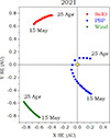 |
Fig. 1. Position of Parker Solar Probe (blue dots), Solar Orbiter (red dots) and Wind (green dots) during the interval 25 April – 15 May, 2021. The plot shows the projection of the orbit on the ecliptic plane in SE (solar ecliptic) coordinates, so that the Sun is at [0,0] (yellow dot). |
The direct alignment is useful, as we show below, because the solar wind measured by the aligned spacecraft originated from the same source of the Sun, and not because they sampled the same plasma parcel.
The magnetic connectivity of the three spacecraft to their solar sources was investigated separately for the two conjunctions using a PFSS model (Schrijver & De Rosa 2003). Indeed, Figure 2 shows the PFSS B2 contour maps and solar wind magnetic footpoints along PSP (blue) and Solar Orbiter (red) trajectories on 30 April 2021 (upper panel); and for Parker Solar Probe (blue) and Earth (green) positions on 07 May 2021 (lower panel). The orbital positions of PSP (blue diamond), Solar Orbiter (red square) and Earth (green dot) were projected, using the ballistic trajectories and measured in situ solar wind speed ±80 km s−1 in bins of 10 km s−1, on the source surface at 2.5 R⊙ and are shown as crosses. These were then connected to the solar wind source regions (circles) calculated for the height R = 1.1 R⊙ using PFSS modeling. Open magnetic field regions are calculated for the height 1.1 R⊙ and are shown in light blue and green colors for negative and positive polarity, respectively, while the neutral lines are shown as bold black lines. These whole sun maps indicate that, on 30 April 2021, PSP and Solar Orbiter were magnetically connected to the same solar wind source region at 1.1 R⊙; and, on 07 May 2021, PSP and Earth were connected to nearly the same area, which, however, evolved over the one-week interval between the conjunctions.
Figure 2 (bottom panels) shows close-ups of the PFSS B2 contour maps presented in Figure 2, with areas of magnetic sources zoomed for detailed view for 30 April 2021 (left panel) and 07 May 2021 (right panel). The symbols used in this figure are the same as those in Figure 2 and the maps were obtained in the same way. They confirm that on 07 May Earth/Wind was connected to the same helio-graphical region as PSP and Solar Orbiter one week earlier. The low corona solar wind sources identified in both zoomed maps are open magnetic field regions in the presence of a pseudostreamer configuration in different stages of evolution.
Pseudostreamer magnetic field configurations often provide favorable conditions for the acceleration of Alfvénic slow wind streams due to the typically very non-monotonic open magnetic field expansion low in the solar corona in the neighborhood of the closed lobe regions (Panasenco & Velli 2013; Panasenco et al. 2019; D’Amicis et al. 2021b).
The 3D magnetic field configurations of the pseudostreamers for both days are presented in Figure 3. The height of the pseudostreamer x-type null point on 30 April (left panel) lies above 1.1 R⊙ and the non-monotonic funnel topology of both adjacent (southern and northern) coronal holes with large non-monotonic expansion factors leads to the formation of the Alfvénic slow solar wind. Even when the overall open field expansion appears modest, when calculated near the source surface, field lines are nearly horizontal, with Br close to zero, at heights of 1.2–1.3 R⊙ in both PS branches. This fast and short over-expansion appears sufficient to lead to slow wind with high Alfvénicity, as illustrated in the left panel of Figure 3. The right panel shows the 3D model for the configuration on May 7. It still has remnants of the pseudostreamer we see on 30 April, but the configuration changed over the week and its x-type null point now is well below 1.1 R⊙; for this reason, Figure 2, right bottom panel shows only one open field area. However, when we take our model below 1.1 R⊙ a pseudostreamer can be seen with a weaker non-monotonic expansion branch in its northern coronal hole. Over the seven days, the pseudostreamer is gradually reducing its magnetic strength, while the surrounding coronal holes slowly merge. The more dynamic and faster moving coronal holes near the equator have a tendency to merge with their polar coronal hole extension counterparts in pseudostreamer formations, erasing the presence of the two neutral lines in the PS base with tripolar configuration.
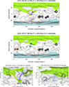 |
Fig. 2. Potential field source surface B2 contour maps and solar wind magnetic foot-points along Parker Solar Probe (blue), Solar Orbiter (red) and Earth (green) trajectories for April 30, 2021 (upper panel) and May 7, 2021 (middle panel). Open magnetic field regions shown in blue (negative) and green (positive), the neutral line is in black bold. Bottom panels: Zoom of each maps of the upper panels for April 30, 2021 (left panel) and May 7, 2021 (right panel). The solar wind source regions (red, blue and green circles) calculated for the height R = 1.1 R⊙. |
 |
Fig. 3. 3D PFSS modeling of the magnetic field lines of two pseudostreamer configurations on April 30, 2021 (left panel) and May 7, 2021 (right panel) using SDO/HMI data. The PFSS reconstructed magnetic field of pseudostreamers is rotated to the limb view, corresponding to a cut along the 150 degree Carrington Longitude in both panels of Figure 2. Green lines are the positive open magnetic field, black lines are closed magnetic field. |
3. In situ observations
3.1. Data description
The following sections focus on in situ plasma and magnetic field data. PSP plasma data were provided by the Solar Wind Electrons Alphas and Protons investigation (SWEAP) (Kasper 2016) which consists of the Solar Probe Cup (SPC), and the Solar Probe Analyzers (SPAN, including SPAN-A and SPAN-B)1. In particular, in this analysis, proton moments (i.e., number density, velocity components and temperature of the main proton population) at 3.5 s are taken from the SPAN-A instrument. The magnetic field is measured by the fluxgate magnetometer of the FIELDS instrument (Bale et al. 2016)2 averaged at the plasma resolution.
Solar Orbiter plasma data are provided by the Solar Wind Analyzer (SWA) (Owen et al. 2020) which consists of the Electron Analyzer System (EAS), the Proton and Alpha Particle Sensor (PAS) and the Heavy Ion Sensor (HIS). In particular, we use data from PAS that measures the 3D velocity distribution functions (VDFs) of protons and alpha particles. We use PAS ground moments (i.e number density, velocity vector, and temperature computed from the pressure tensor) derived from the VDFs at 4 s resolution. Magnetic field measurements are provided by the Magnetometer (MAG) instrument (Horbury et al. 2020), averaged at the plasma sampling time. Data are available on the Solar Orbiter Archive3.
Plasma data from Wind are obtained from the Three-Dimensional Plasma and Energetic Particle Investigation (3DP) (Lin 1995) and magnetic field data from the Magnetic Field Investigation (MFI) (Lepping 1995) instrument, averaged at the plasma sampling time4. In this paper, we use the 3DP ground moments at about 24 s resolution to show the overview time series, while the spectral analysis is performed using 3DP onboard moments at 3 s resolution, which are not used for showing time series because of quantization affecting onboard moments.
3.2. Conjunction between Parker Solar Probe and Solar Orbiter on April 30, 2021
Figure 4 shows PSP time series of relevant parameters covering day 30 April 2021, just after PSP passed its 8th perihelion. From top to bottom, this figure displays: the solar wind bulk speed, Vsw, in km/s; the velocity-magnetic field (v-b) correlation coefficient, Cvb, computed at 30 min scale using a running window, which corresponds to a typical Alfvénic scale (e.g., Marsch & Tu 1990); the radial component of the magnetic field, BR in nT; the angle the magnetic field forms with the velocity field, ΘVB in degree; the magnetic compressibility, measured by the square root of the ratio between the variance computed on the magnetic field magnitude over the sum of variances of the components, σB2/∑iσBi2, computed at 30 min scale; the plasma β. The gray box highlights the portion of the solar wind connected to the solar source in Figure 2 when PSP was located at 0.10 au. If we consider the fields V and B as a superposition of a background mean field and fluctuations, namely B = B0 + b and V = V0 + v, θVB is defined as the angle between V and B vectors. The correlation coefficient Cvb is computed from the Pearson’s correlation between the v-b fluctuating fields only, since the average field is subtracted within each 30-minute interval, so the resulting correlation reflects only the fluctuations of the field rather than the full vector alignment.
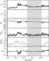 |
Fig. 4. First conjunction: Parker Solar Probe time series of relevant parameters. From top to bottom: solar wind bulk speed, Vsw, in km/s; v-b correlation coefficient computed at 30 min scale using a running window, Cvb; radial component of the magnetic field, BR in nT; angle the magnetic field forms with the velocity field, ΘVB in degree; magnetic compressibility, σB/σbi computed at 30 min scale; plasma beta β. The gray box identifies the connected solar wind when PSP was at 0.10 au from the Sun. |
This interval is characterized by slow wind (bulk speed less than 400 km/s) showing one-sided velocity fluctuations (Gosling et al. 2009) similar to what is observed in the fast wind, although with smaller amplitude fluctuations than the fast wind at those heliocentric distances.
The correlation coefficient Cvb is computed over the three v-b components separately using a running window of 30 min length and it is then defined as the average value of the three components ∑i = R, T, NCvbi/3. The sign of correlation is given by −sign(V ⋅ B). Since V is always positive, if the magnetic field has a negative polarity (B < 0), V and B components are correlated (Cvb > 0) while if the magnetic field polarity is positive, V and B components are anticorrelated (Cvb < 0) as in this case. It shows values close to −1, which are also related to low magnetic compressibility, indicating that fluctuations in the magnitude of the total magnetic field are much smaller than the magnitude of the field fluctuations, which is a typical signature of Alfvénic fluctuations.
The beginning of this interval was also studied in Bandyopadhyay et al. (2022), with the aim of characterizing turbulence properties of solar fluctuations in sub-Alfvénic intervals. Indeed, it was found to have Alfvén Mach number less than 1 and turbulent properties that differ from the typical super-Alfvénic ones (see paper for details).
Figure 5 shows Solar Orbiter time series of the same parameters presented in Figure 4 from 29.6 to 30.6 April 2021 during which the s/c was located at about 0.89 au from the Sun. The gray box identifies the portion of the solar wind connected to the solar source in the upper panel of Figure 2.
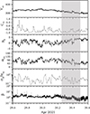 |
Fig. 5. First conjunction: Solar Orbiter time series of relevant parameters at 0.89 AU, similar to Figure 4. The gray box identifies the connected solar wind. |
This interval is characterized by a slow wind with bulk speed ranging from 300 km/s. Also in this case, Cvb is computed at 30 min scale and it is generally more fluctuating than in the Parker Solar Probe case, suggesting that Alfvénic fluctuations are less pure. This is also confirmed by the higher and more oscillating compressibility than the PSP case, ranging between 10−2 and 10−1, although still much less than 1. Focusing on the gray box, Cvb is found to be rather high (in absolute value) although less stable than the PSP case.
By inspecting the behavior of the plasma β, during the conjunction, in the blue shaded area of Figure 4, β remains around a stable value of ∼10−1. After the expansion at the Solar Orbiter position, the β parameter shows larger fluctuations and reaches greater values around 1.
3.3. Conjunction between Parker Solar Probe and Wind on May 7, 2021
During the second conjunction, PSP was at a heliocentric distance of 0.33 au. Although the average bulk speed was found to be around 277 km/s (as shown in Table 1), poor-quality plasma data did not allow us to use all the parameters shown for the first conjunction. Therefore, Figure 6 shows only BR, the magnetic field magnitube, B, and the magnetic field compressibility. The box identified in gray marks the back-mapped interval, characterized by a well-defined magnetic polarity. The indirect presence of Alfvénic fluctuations is suggested by a constant magnetic field magnitude, large amplitude fluctuations and low compressibility.
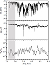 |
Fig. 6. From top to bottom: time series of BR, B and magnetic compressibility measured by PSP at 0.33 au during the second conjunction. The gray box is the connected solar wind. |
Figure 7 shows Wind time series of relevant parameters from 6.8 to 7.8 May 2021 similar to what is shown in Figures 4 and 5. The gray box identifies the portion of the solar wind connected to the solar source in the lower panel of Figure 2. In this case, Cvb is close to −1 and looks less fluctuating than in the Solar Orbiter case, indicating a slightly different Alfvénic character of the fluctuations, probably due to the different evolution of the source region from April 30 to May 7. This could explain the much lower density, higher Alfvén speed and lower plasma β observed at the Wind location.
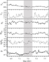 |
Fig. 7. Second conjunction: Wind time series of relevant parameters at 1.0 AU, similar to Figure 4. The gray box is the connected solar wind. |
4. Characterizing solar wind fluctuations
4.1. Spectral analysis of the solar wind streams
The solar wind velocity and magnetic field fluctuations show a self-similar behavior over several frequency decades. Their power spectra are characterized by power laws. Alfvénic intervals, in particular, are typically characterized by at least three frequency ranges:
-
The f−1 regime is observed at low frequencies (or large scales), and its origin is still debated. Several hypotheses have been proposed over the years, such as: the effect of superposed uncorrelated samples of turbulence of different solar origin (Matthaeus & Goldstein 1986), the signature of an inverse cascade of low-frequency modes (Dmitruk & Matthaeus 2007), the outward propagating modes reflected by large-scale solar wind gradients in the extended solar corona (Verdini et al. 2012), or more recently, the saturation of the magnetic field fluctuations to the amplitude of the local magnetic field (Matteini et al. 2018; Bruno et al. 2019; D’Amicis et al. 2020; Perrone et al. 2020).
-
The intermediate range, commonly referred as inertial range, shows a typical power law spectrum (Coleman 1968), which is generally characterized by a Kolmogorov scaling of f−5/3 in magnetic field fluctuations (Bruno & Carbone 2013), or an Iroshnikov-Kraichnan scaling of 3/2 within 1 au (Podesta et al. 2006, 2007; Salem et al. 2009; Borovsky 2012; D’Amicis et al. 2020) in velocity fluctuations (although it evolves toward an f−5/3 beyond the Earth’s orbit as shown by Roberts et al. 1987a). Observations by PSP based on a global survey of solar wind data have demonstrated that power spectra of magnetic field fluctuations undergo a radial evolution of the slope ranging from f−3/2 close to the Sun to a f−5/3 toward 1 au (Alberti et al. 2020; Chen et al. 2020). However, more recent observations based on single streams in different solar wind conditions have shown that the two scalings can coexist, thus constituting two sub-ranges at inertial scales, where the f−3/2 spectrum is observed at lower frequencies, whereas f−5/3 develops at higher ones (Telloni 2022; Sioulas et al. 2023; Wu et al. 2023; Mondal et al. 2025; D’Amicis et al. 2025; Wu et al. 2025; Sioulas et al. 2025).
-
Around proton scales, Leamon et al. (1998) and Smith et al. (2006) observed steeper spectra with a large variability of the spectral slope, between −3.75 and −1.75. Bruno et al. (2014) highlighted a transition of the spectral slope when moving along the trailing edge of the fast streams, where the speed is higher, and the lowest values appear within the subsequent slow wind, followed by a steeping of the spectra in the trailing edge of the fast streams. The spectral index seems to depend on the power characterizing the fluctuations within the inertial range: the higher the power, the steeper the slope, as also confirmed by D’Amicis et al. 2019. In particular, this slope tends to approach −5/3 within the slowest wind and a limiting value of −4.37 within the fast wind.
This section presents a spectral analysis to highlight similarities and differences in velocity and magnetic field fluctuations for the selected intervals observed by PSP, Solar Orbiter, and Wind. In this analysis we used higher-resolution Wind plasma data, i.e., 3 s corresponding to the onboard plasma data sampling time, to cover a larger frequency range comparable to those of PSP and Solar Orbiter. Plasma data at this sampling time show digitalization effects, which, however, do not affect power spectral density analysis (see also D’Amicis et al. 2020, and reference therein). Power spectral densities (PSDs) of velocity and magnetic field fluctuations are shown in Figure 8 for three different streams. The magnetic field PSDs are presented in the top panels along with a piecewise fit showing how the inertial frequency interval can be consistently described by two different scaling laws. A clear 1/f spectrum is observed at Wind and PSP, whereas Solar Orbiter exhibits a spectral bump possibly due to some large-scale drivers introducing some power at a specific scale in the detected fluctuations. However, the investigation of large-scale phenomena is beyond the scope of the present paper. Concerning PSP observation, we emphasize that in this case we clearly observe a well developed 1/f range close to the Sun at 0.1 au. This observation is consistent with recent findings reported by Huang et al. (2023) based on PSP data. Due to the reduced plasma resolution, the ion scales are not well-resolved. In Table 1, the resonance damping frequency, fR, was inserted for reference as a typical scale where the transition between fluid and kinetic scales in solar wind velocity and magnetic field power spectra may occur (Leamon et al. 1998; Bruno & Trenchi 2014; Telloni et al. 2015; Woodham et al. 2018; Wang et al. 2018; D’Amicis et al. 2019). For this reason, we limited our analysis to the MHD scales by resampling magnetic field data at the same cadence of the plasma data gathered by the three probes.
Bulk parameters averaged over the selected intervals.
Also in the case of velocity fluctuations (Figure 8 lower panels), the low frequency 1/f slope is clearly observed in PSP and Wind data samples, whereas the trend observed in the Solar Orbiter PSD resembles the property discussed for the magnetic field. At MHD scales, the slopes are generally shallower with respect to the magnetic field, with a clear onset of the instrumental noise toward the lower end of the inertial range, except for PSP. In the latter case, the power associated with the large amplitude fluctuations observed near the Sun in the higher frequency part of the spectrum exceeds the noise floor, revealing a clear Kolmogorov-like trend.
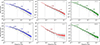 |
Fig. 8. PSD of the trace of B (top panels) and V (bottom panels). The gray lines indicate the full-frequency PSD, whereas the blue, red and green lines are the corresponding PSDs smoothed through the Welch’s method. Darker blue, red and green solid lines indicate the piecewise fits performed in different frequency intervals as marked by vertical dotted lines. Sectors where power-law fits are missing are strongly affected by instrumental noise. |
In the turbulent domain, we identify two sub-ranges in the PSDs of magnetic field and velocity fluctuations, characterized by a shallower slope at lower frequency, close to the one predicted by the Kraichnan theory, and a steeper slope at higher frequencies, resembling the Kolmogorov scaling f−5/3. To highlight the emergence of the two sub-ranges at inertial scales in Figure 8, we overlay the smoothed trend of the PSDs of B and V obtained by applying the Welch’s method to the full-range PSDs. This makes the transition clearly visible, as also emphasized by the piecewise power-law fits reported in the figure. This scenario is consistent with recent observations by D’Amicis et al. (2025), based on Solar Orbiter perihelion data, as well as with observations in different points of the heliosphere, such as PSP, Helios, and Ulysses (Mondal et al. 2025; Wu et al. 2025; Sioulas et al. 2025).
Figures 4, 5 and 7 show high values of Cvb and low compressibility, CB = σB/∑iσBi corresponding to fluctuations with a high Alfvénic correlation. However, Cvb and CB have been computed at a single Alfvénic scale, i.e., 30 min, which falls within the inertial range. Although Helios observations have shown that the most Alfvénic range of scales typically extends from tens of minutes to hours (Bruno 1985; Marsch & Tu 1990), the Alfvénic content of the fluctuations depends not only on the scale but also on the distance from the Sun and on the type of solar wind regime observed (Bruno & Carbone 2013). The complete range of Alfvénic scales can be identified through the spectral analysis of the Elsässer variables, z± (Elsässer 1950; Marsch & Tu 1990). These quantities are defined as z± = v ± b, where b is the magnetic field vector in Alfvén units, when the background magnetic field points toward the Sun, while z± = v ∓ b for the opposite polarity. Hence, z+ always identifies outward propagation modes while z− identifies inward fluctuations. Used for the first time to investigate solar wind turbulence by Tu et al. (1989) and Grappin et al. (1991), the Elsässer variables constitute a useful tool to visualize and quantify whether solar wind fluctuations contain Alfvénic correlations.
We first estimated the three components of z+ and z− in RTN coordinates for PSP and Solar Orbiter and GSE coordinates for Wind, and computed the PSD of each component. Figure 9 shows the trace of the power spectral density of the components, e± vs f, which identifies the energy associated with these propagating modes (either inward or outward).
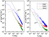 |
Fig. 9. Power spectra of e+ (left) and e− (right) corresponding respectively to PSP (blue), Solar Orbiter (red) and Wind (green) intervals identified in gray in Figs. 4, 5 and 7. |
We then computed the normalized cross-helicity in the frequency domain using the definition: σC(f) = (e+(f)−e−(f))/(e+(f)+e−(f)), as shown in the upper panel of Figure 10, for the three s/c (same color code used throughout the paper). By definition, σC measures the balance between the outward propagating mode with respect to the inward propagating one. In this view, σC equal to 1 (−1) indicates the presence of only the outward (inward) component, while |σC|< 1 corresponds to a mixture of both modes and/or non-Alfvénic fluctuations. It must be noted that σC is strongly linked with the v-b correlation coefficient via the following relation: Cvb = σC/(1 − σR2)1/2, indicating that σC is equal to Cvb only in the case of energy equipartition, σR = 0.
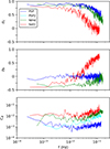 |
Fig. 10. From top to bottom: Power spectra of the normalized cross-helicity, σC, normalized residual energy, σR, and magnetic compressibility, CB, corresponding respectively to PSP (blue), Solar Orbiter (red) and Wind (green) intervals identified in cyan in Figs. 4, 5 and 7. The cyan line in the bottom panel is the power spectrum of the magnetic compressibility of PSP on May 7, 2021 (see interval identified by the cyan box in Figure 6). |
As expected, PSP shows the highest values of σC. The extension of the Alfvénic range, indicated as the frequency range for which σC > 0.75 for reference, reaches values up to 4 × 10⁻² Hz (corresponding to 25 s) at PSP, while it is reduced to the frequency range 1 × 10⁻⁴–8 × 10⁻³ Hz (corresponding to time scales ranging from 2 to almost 3 h) and 2 × 10⁻⁴–3 × 10⁻² Hz (corresponding to time scales ranging from 30 s to 1.30 h), for Solar Orbiter and Wind respectively. In general, we also observe a decrease in the value of σC at MHD scales as we move away from the Sun. This trend is expected for larger and larger time scales (Roberts et al. 1987a), or lower and lower frequencies in Figure 10. By comparing Figures 9 and 10, we can notice that the evolution of σC is mainly due to a decrease in the power associated with e+ when moving from PSP to Solar Orbiter or Wind. This seems to be in agreement with the findings by Bruno & Bavassano (1993), attributing this behavior to the interaction between Alfvénic fluctuations with static structures or magnetosonic perturbations, able to modify the homogeneity of the background medium, on a scale comparable to the wavelength of the solar wind fluctuations. On the other hand, a decrease in σC might be interpreted as an increase of inward modes produced, for example, within velocity shears where some plasma instability may be active (Matthaeus et al. 1982; Roberts et al. 1987a,b; Grappin & Velli 1996; Bavassano et al. 2000; Matthaeus et al. 2004), although Bavassano & Bruno (1989b) related the decrease of Alfvénicity to magnetic field and/or density enhancements most of the time, that would determine a decrease outward modes rather than the local generation of inward modes (Bavassano & Bruno 1989a; Bruno & Bavassano 1991).
We then considered the trace of the power spectral density of V (left bottom panel in Figure 7) and computed that of B in Alfvén units (indicated as ev(f) and eb(f), respectively) in order to evaluate σR(f) = (ev(f)−eb(f))/(ev(f)+eb(f)) (Tu & Marsch 1995), i.e., the imbalance between kinetic and magnetic energy in the frequency domain. σR equal to 1 (−1) indicates a kinetic (magnetic) energy imbalance, while σR = 0 corresponds to equipartition of energy and characterizes pure Alfvénic fluctuations. The most Alfvénic frequency range in PSP observations shows also quasi-equipartition of energy with σR ∼ 0. On the other hand, Solar Orbiter and Wind observations show a clear imbalance in favor of magnetic energy, resulting in σR between −0.3 and −0.4. This is confirmed by Bruno (1985) at a distance close to 1 au using Helios data, studying the Alfvén ratio rA. This quantity is the ratio between kinetic energy and magnetic energy in Alfvén units, ev/eb, and it is linked to σR by (rA − 1)/(rA + 1)). In addition, Belcher & Davis (1971), Solodyna & Belcher (1976), Matthaeus et al. (1982) showed that rA is usually < 1 and reaches a limit value around 0.45 at some au (Matthaeus et al. 1982; Roberts et al. 1990). This corresponds to a limit value of σR around −0.38, which is in agreement with our findings in this range of heliocentric distances. However, it must be noted that, beyond 30 au, in the outer heliosphere, Adhikari et al. (2015, 2017) found that the rA reverses its trend compared to what is observed in the inner heliosphere approaching 1, while σR changes accordingly, tending toward 0.
The lack of energy equipartition of solar wind fluctuations is still an open issue. Although numerical simulations by Matthaeus & Goldstein (1986) and Mininni et al. (2003) predict rA < 1, the results do not discard either a final excess of kinetic energy. On the other hand, also corrections related to the presence of alpha particles, or anisotropy in the thermal pressure (Belcher & Davis 1971) or the three fluid effect (Bavassano & Bruno 2000) are not able to explain the observed magnetic excess of the fluctuations. The increasing magnetic imbalance might be due either to a natural evolution of turbulence which might determine a final state dominated by magnetic energy (Grappin et al. 1991; Roberts et al. 1992; Roberts 1992; Mininni et al. 2003) or to an increase in the occurrence of magnetic structures (e.g., Tu & Marsch 1993).
Alfvénic turbulence is characterized not only by high v-b correlations but also by weak magnetic compressibility. Indeed, fluctuations in the magnitude of the total magnetic field are much smaller than the magnetic field fluctuations and fluctuations are considered to remain in a state of spherical polarization (Bruno et al. 2007; Matteini et al. 2015). This basically motivates the bottom panel showing magnetic compressibility defined as the ratio between the PSD of the magnitude of magnetic field over the trace of PSD of the magnetic field vector. In this panel, we observe an evolution toward an increase of magnetic compressibility as the Alfvénic content of the fluctuations decreases, basically confirming the findings by Telloni et al. (2021), in agreement with the decrease of Alfvénicity with the heliocentric distance. Only this quantity, relying on magnetic field measurements only, can be represented for the second PSP data sample (gray), due to the lack of plasma measurements.
As we move toward higher frequencies, caution is needed to interpret the high-frequency part of the PSDs reported in Figure 10, since it is due to the noise of plasma sensors. Indeed, the decrease of σC is associated with a flattening of e− rather than a decrease of e+ (see Figure 9). The tendency of σR to become positive, is related to a flattening of ev, due to instrument noise (for frequencies > 0.02 Hz), rather than a decrease of eb (see Figure 8). This is particularly true for Solar Orbiter, but the same effect is present also in Wind (see also D’Amicis et al. 2022).
4.2. Intermittency
When a nonlinear cascade of energy generates a Kolmogorov spectrum, the spatial distribution of the turbulent fluctuations becomes increasingly inhomogeneous as the scale decreases. Such phenomenon, known as intermittency in fully developed turbulence (Frisch 1995), arises from the properties of the nonlinear interactions and leads to efficient energy dissipation in localized small-scale, large amplitude structures, which occupy a small fraction of the volume. Quantitative analysis of intermittency in solar wind turbulence was used to characterize different regimes and plasma conditions, and represents a crucial tool for the correct description of the evolution of turbulence in the solar wind expansion (see Bruno 2019, and references therein). The standard tool to measure intermittency are the structure functions, Sq(Δt) = ⟨Δϕq⟩∼Δtζq, where Δϕ = ϕ(t + Δt)−ϕ(t) are scale-dependent increments of the field ϕ at a lag Δt (where the Taylor hypothesis is assumed to switch form time to space lags, Taylor 1938; Perri et al. 2017). The set of scaling exponents ζq captures the scale-dependent statistical properties of the increments (see Frisch 1995; Bruno & Carbone 2013, and references therein). A more compact estimator of intermittency is the flatness (or kurtosis), defined as the standardized fourth-order moment of the fluctuations, F(Δt) = S4/S22. Such statistical quantity describes the scale-dependent shape of the increments’ distribution function. For Gaussian-distributed increments, such as the uncorrelated large-scale fluctuations, F = 3. In a turbulent cascade, the flatness then increases as the lag decreases, marking the emergence of intense, localized and rare structures, which raise the tails of the distributions (Sorriso-Valvo et al. 1999; Bruno et al. 2003). Since both the fourth and second order structure functions have power-law scaling in the inertial range, their ratio will also scale as a power law, F ∼ Δt−κ. The scaling exponent κ = −ζ4 + 2ζ2 can be used to quantitatively estimate the relevance of intermittency in spacecraft measurements. In Navier-Stokes turbulence, the velocity typically has κ ≃ 0.1 (Anselmet et al. 1984), while in solar wind turbulence steeper power laws are observed for both velocity and magnetic field, κ ≃ 0.2 − 0.5 (Sorriso-Valvo et al. 2023). In Figure 11, we show the scale-dependent flatness of magnetic field (top) and velocity (bottom) fluctuations for PSP (left), Solar Orbiter (center) and Wind (right). In all the above panels, the same colors as in previous figures indicate the different intervals, and the horizontal dashed lines mark the reference Gaussian value, F = 3. Ranges of power-law scaling are identified in the MHD domain, often with a break separating two different sub-ranges, indicated by vertical lines. The double scaling range was recently observed in several samples of Alfvénic solar wind, and indicates that the more Alfvénic turbulence developed at larger scales tends to reduce the alignment between velocity and magnetic field fluctuations at smaller scales, evolving in a more fluid-like turbulence. These features thus coexist within the inertial range of solar wind (Wicks et al. 2011; Telloni 2022; Sorriso-Valvo et al. 2023; Sioulas et al. 2023; Wu et al. 2023; Mondal et al. 2025; D’Amicis et al. 2025; Wu et al. 2025). In the figure, the fits are represented by solid lines, and the corresponding exponents κ are given in colors. At PSP, in the smaller-scale MHD sub-range, where velocity and magnetic spectral exponents are close to Kolmogorov’s 5/3, the scaling exponents are compatible with previous observations in similar contexts, and indicate strong intermittency at all distances from the Sun. In the larger-scale sub-range, roughly corresponding to the 3/2 spectral range, a shallower power-law scaling is present, indicating reduced intermittency associated with more Alfvénic turbulence. For Solar Orbiter, magnetic field, the double scaling was not observed, but rather a single range emerged covering both sub-ranges emerging from the spectral analysis. This is in disagreement with previous observations (Telloni 2022; Sorriso-Valvo et al. 2023; Sioulas et al. 2023; Mondal et al. 2025; D’Amicis et al. 2025), and might be related to the presence of a few sharp mesoscale structures visible in the time series. Solar Orbiter velocity also presents one single scaling range with moderate intermittency, with small scales dominated by the noise. At Wind, the magnetic field again shows one single inertial range (there is no clear break visible around Δt ≃ 100 s, as observed in the spectrum). However, the range of scales corresponding to the 1/f spectral range shows power-law scaling. This was previously observed in Helios data (Sorriso-Valvo et al. 2023), and suggests that even the low-frequency range typically associated with uncorrelated fluctuations include weaker yet effective nonlinear interactions (Dmitruk & Matthaeus 2007; Verdini et al. 2012; Matteini et al. 2018). Finally, as for PSP, the flatness of the velocity shows a break in the middle of the inertial range, corresponding to the observed break between the 3/2 and 5/3 spectral sub-ranges.
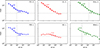 |
Fig. 11. Scaling of the flatness, F(Δt), for the intervals measured by PSP (left panels), Solar Orbiter (central panels) and Wind (right panels). The flatness was averaged over the three components of magnetic field (top panels) and velocity (bottom panels). Power-law fits F ∝ Δt−κ are indicated (solid lines), together with the corresponding scaling exponent κ. The horizontal dashed gray line indicates the Gaussian reference value F = 3. When a break separates the two scaling ranges, vertical dashed lines indicate its time scale. |
In contrast with previous observations (Telloni 2022; Sorriso-Valvo et al. 2023; Mondal et al. 2025), there is no apparent dependency of intermittency on the heliocentric distance in the Kolmogorov range. This suggests that for the present interval the intermittency evolution might not be determined solely by the expansion and by the associated natural decay of the fluctuations. Other factors, such as local interactions with the surrounding plasma or with the heliospheric current sheet, might contribute to modify the intermittency and the efficiency of dissipative processes. However, in the lower-frequency (Alfvénic turbulence) range intermittency increases considerably from PSP to Solar Orbiter and Wind, indicating that in this range the radial evolution of the turbulent cascade is more evident. Moreover, in the same range of scales we observe a radial evolution of σC and σR, as reported in Section 4.1, characterized by a decay of the v-b alignment and a corresponding dominance of the magnetic energy at Solar Orbiter and Wind. The concurrent increase in the intermittency suggests that Alfvénic fluctuations can be weakened by the interaction with the turbulent structures that emerge in the MHD range as the distance from the Sun increases.
5. Energy transfer
In the MHD inertial range, the turbulent energy cascade described in previous sections can be examined in more quantitative detail by means of the Politano-Pouquet (PP) law (Politano & Pouquet 1998). In its simplest version, such law, obtained from the MHD equations under the assumption of homogeneity, stationarity, isotropy, incompressibility and large Reynolds’ number (for a discussion on the alternative versions of the PP law, see Marino & Sorriso-Valvo 2023, and references therein), prescribes the linear scaling of the mixed third-order structure function
 (1)
(1)
In Equation (1), ΔϕL indicates longitudinal increments of the component of a generic scalar or vector component, ϕ, along the sampling direction. The mean solar wind speed, Vsw, is used to switch between spatial scales, Δl, to temporal scales, Δt, so that, under the usual assumptions of the Taylor hypothesis, Δl = −VswΔt (Taylor 1938). The PP law has been applied in various space environments, spanning from the sub-Alfvénic solar wind (Zhao et al. 2022) to the inner and outer heliosphere (e.g., Sorriso-Valvo et al. 2007; Bandyopadhyay et al. 2020; Wu et al. 2022; Sorriso-Valvo et al. 2023), and to planetary environments (Hadid et al. 2018; Andrés et al. 2020; Richard et al. 2024). The intervals studied here display different data quality levels, which affects the possibility to observe the PP law. Only the PSP interval of April 30, 2021 presents no issues, and provides sufficient data resolution and statistical convergence for the correct determination of the energy transfer rate (Dudok De Wit 2004). Unfortunately, as remarked before, the Solar Orbiter plasma measurements suffer from severe instrumental noise at scales smaller than 200 s (see for example the spectral and flatness flattening). This makes the estimates of the PP law incomplete in the inertial range. Indeed, it is likely that the energy term of Equation (1) (the first of the two right-hand-side terms), which is usually the dominating positive contribution and accounts for energy transfer associated to velocity gradients, vanishes due to the random velocity fluctuations. On the other hand, the typically negative cross-helicity term (the second of the two right-hand-side terms), which accounts for the transfer of correlated velocity and magnetic field fluctuations associated to magnetic gradients, may still contribute to the linear scaling. To improve statistical convergence, the Wind interval was extended to include the neighboring plasma measured from May 5 to May 8. This results in the inclusion of non-Alfvénic portions of solar wind. Additionally, as we have seen in Section 3, the source region has probably evolved and cannot be considered as strictly stationary during the two observations. Finally, the PSP 7 May 2021 interval was obviously excluded for the complete lack of plasma data.
With the above caveats, we computed the mixed third-order moments Y(Δt) for the three indicated samples. A broad range of linear scaling with fixed sign of Y(Δt) emerges for the PSP and Solar Orbiter samples, as shown in the top panel of Figure 12. The third-order moments for Solar Orbiter are negative, as could be expected since the velocity-gradient contribution is dominated by noise. For the Wind interval, the linear scaling is not as clear and only extends to slightly less than one decade. In all cases, a break in the linear scaling is observed around Δt ≃ 200 s, approximately compatible with the observed break in the PSD and in the flatness (∼100 s). Hence, linear fits were performed between a few seconds and such break, corresponding to a few minutes. For PSP and Wind, such scales match the spectral range where the Kolmogorov (or Kraichnan) scaling are observed (see Figure 8), and the smaller-scale sub-range for the flatness. At larger scales, including the larger-scale intermittency sub-range and typically extending in the 1/f spectral range, the PP law is not verified (Sorriso-Valvo et al. 2023). This suggests that in the 3/2 spectral range the turbulence might not satisfy all the requirements for the PP law (for example, isotropy), which are met in the 5/3 region. The fitting coefficients obtained in the inertial range were then used to estimate the energy transfer rate, ε, indicated next to each fit in MJ kg−1 s−1. Although only the estimate at PSP is reliable, the values measured at the three spacecraft are broadly consistent with previous observations at similar distances from the Sun (Smith et al. 2009; Hernández et al. 2021; Zhao et al. 2022; Sorriso-Valvo et al. 2023; Brodiano et al. 2023; Marino & Sorriso-Valvo 2023).
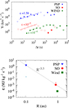 |
Fig. 12. Top panel: scaling of the mixed third-order moment, Y(Δt), for the intervals measured by PSP (blue triangles), SO (red circles) and Wind (black squares, estimated using a 3-day extended interval). Positive and negative values are indicated with full and open markers, respectively. Linear fits are indicated (gray lines), and the resulting energy transfer rates, ε, are indicated in MJ kg−1 s−1 (color coded). Bottom panel: estimated turbulent energy transfer rate versus radial distance from the Sun, for PSP, SO and extended Wind intervals (same colors as in the top panel). A power-law (dashed line) with decay exponent -3.3 (fitting PSP and SO transfer rates at the first alignment) is shown for reference. The smaller, lighter symbols indicate the estimated turbulent heating rate εT. |
In the bottom panel of Figure 12, we plot the magnitude of ε for the three cases as a function of the distance from the Sun. Using the values at the alignment between PSP and Solar Orbiter, and assuming power-law radial decay, a fit of the two values obtained from PSP and Solar Orbiter would provide the decay exponent −3.3, suggesting that the energy of the magnetohydrodynamic fluctuations has been rapidly removed from the system during the expansion. This estimate should be considered as an order of magnitude reference, with the important caveat that the value obtained at Solar Orbiter may be affected by the plasma instrument noise. For the Wind interval, the measured energy transfer is even smaller, which would correspond to a steeper decay when the PSP value at the first alignment is considered. However, as noticed above, the extended Wind interval includes portions of non-Alfvénic solar wind, and the coronal source region appears to have undergone some topology evolution between the two observations. For comparison, the decay exponent obtained here is considerably larger than those previously estimated using recurrent streams measured by Helios 2, which were reported as −1.83 and −2.33 for fast Alfvénic and slow non-Alfvénic solar wind, respectively (Sorriso-Valvo et al. 2023). Using the average proton temperature and speed at the two aligned points, T(R) and Vsw(R), and the cooling rate obtained fitting the temperature profile to a power law T(R)∝R−ξ (Smith et al. 2006b; Sorriso-Valvo et al. 2023), it is possible to estimate the turbulence heating rate, εT, representing the turbulent energy that must be dissipated into heat to provide the observed proton temperature non-adiabatic decay. The heating rate was modeled by Verma and Vasquez as (Verma et al. 1995; Vasquez et al. 2007):
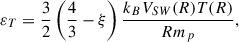 (2)
(2)
where kB is the Boltzmann constant and mp is the proton mass, and the decay exponent obtained for the PSP-SO alignment is ξ = 0.23, indicating a very slow cooling. Because of the lack of PSP plasma parameters, we could not estimate the cooling and turbulent heating rates for the alignment between PSP and Wind. The turbulence heating rates from the Verma-Vasquez model (2) are shown in the bottom panel of Figure 12 as smaller symbols and in lighter colors with respect to the energy transfer rate. At PSP, the modeled heating is two orders of magnitude smaller than the available turbulent energy transfer rate, while at Solar Orbiter it is slightly larger. Such excess of energy at PSP could result in different forms of plasma energization, not examined here.
6. Summary and conclusions
In this paper, we focus on a particular orbital configuration involving PSP during E8, Solar Orbiter at 0.89 au and Wind, over about a week. Remarkably, the different plasma parcels observed by all the s/c originated from the same solar source region, allowing us to study not only the evolution of the solar wind detected in situ but also of its solar source, using different s/c at different heliocentric distances and different times. Each s/c observed a slow wind with a different Alfvénic content of the fluctuations. The first conjunction in particular identifies an open field region of the solar wind sources characterized by a well-developed pseudostreamer configuration with strong non-monotonic expansion of the open magnetic field. The gradual evolution of this pseudostreamer created opportunity to sample the solar wind from its decaying configuration a week later during the second conjunction. The collapsing pseudostreamer configuration allowed us to follow and connect in situ data with the evolution of the large-scale coronal configurations of magnetic funnels formed as parts of the pseudostreamer topology.
Solar wind fluctuations were characterized performing a spectral analysis with the aim to study the evolution of the Alfvénic range. This task was performed by studying σC, σR and CB in the frequency domain. Previous studies related to the Helios mission, spanning heliocentric distances from 1 au and as close as 0.29 au, have shown that the Alfvénic range typically extends from tens of minutes to hours (Bruno 1985; Marsch & Tu 1990). Our analysis shows that we can further extend the Alfvénic range to tens of sec when the s/c is closer to the Sun. Indeed, as expected, PSP shows the highest value of Alfvénicity that results not only in high v-b correlations but also in the largest amplitude fluctuations. This occurs in the widest range of scales, up to 4 × 10⁻² Hz, corresponding to a time scale of 25 s. On the other hand, the Alfvénic range is reduced at Solar Orbiter and Wind locations to the frequency range 1 × 10⁻⁴ − 8 × 10⁻³ Hz and 2 × 10⁻⁴ − 3 × 10⁻² Hz, respectively. Although the comparative spectral analysis seems to clearly show different extensions for the Alfvénic ranges for the different streams, the shrinking of the frequency range far away from the Sun is also due to instrumental noise affecting some plasma instruments at high frequency, especially for Solar Orbiter and Wind measurements.
In addition, the spectral analysis clearly shows the evolution of the energy partition in solar wind fluctuations with the heliocentric distance. While magnetic and velocity fluctuations observed at PSP are in equipartition of energy, Solar Orbiter and Wind observations show a clear magnetic energy imbalance in agreement with previous findings (e.g., Matthaeus et al. 1982; Bruno 1985; Roberts et al. 1990). This is not surprising since PSP spans heliocentric distances that have not been explored before and investigates a region close to the Sun where we expect Alfvénic fluctuations to dominate and to be purer. The lack of energy equipartition far from the Sun is still not fully understood. Indeed, although we take into account also the presence of alpha particles, or anisotropy in the thermal pressure (Belcher & Davis 1971) or the three fluid effect (Bavassano & Bruno 2000), we would not be able to fully correct the observed magnetic excess of the fluctuations. This is probably due to a natural evolution of turbulence which might determine a final state dominated by magnetic energy (Grappin et al. 1991; Roberts et al. 1992; Roberts 1992; Mininni et al. 2003) or to an increase of emergence of magnetic structures (e.g., Tu & Marsch 1993). The decrease of Alfvénicity with the heliocentric distance is also accompanied by an increase of magnetic compressibility, as expected, confirming previous findings by Telloni et al. (2021).
The properties of turbulence were also described through the level of intermittency, estimated using the power-law scaling law of the flatness of the fluctuations. A double scaling range was identified for the magnetic fluctuations at PSP, but not at Solar Orbiter and Wind. For the velocity, the double scaling was observed at PSP and Wind. The intermittency did not show evident radial evolution in the higher-frequency part (i.e., the Kolmogorov-like spectrum) of the inertial range, which appears to be in contrast with previous observations of clearly evolving intermittency. However, we observe an increasing level of intermittency in the Alfvénic turbulence range (where the spectral exponent is 3/2), as the distance from the Sun increases, associated with a degradation in the v-b correlation and with a predominance of magnetic energy. This suggests that pristine Alfvénic fluctuations observed at 0.1 au then interact with the structures of the developing turbulence.
Finally, we estimated the cross-scale turbulent energy transfer rates via the third-order moment scaling law, and its radial decay. Although with some degree of uncertainty due to non optimal experimental conditions, we observed a faster energy decay compared to previous observations, indicating a possible rapid energy dissipation in this particular sample. In order to determine if and how such fast decay depends on solar wind parameters, more cases will need to be studied.
This study represents a good example of solar wind parcels observed by different s/c connected to the same solar source that evolves over a week. The stationarity or evolution of the solar source could partly explain why Alfvénicity can be maintained or lost within slow solar wind streams when observed at different heliocentric distances (e.g., D’Amicis et al. 2021a). However, in addition to the conditions at the origin, one should also take into account local inhomogeneities that would determine the degradation of v-b correlations as, for example, the presence of compressible phenomena (e.g., Bruno & Bavassano 1991). The investigation of similar case studies (evolution of the solar source) or radial alignments (evolution of the same plasma parcel) involving PSP, Solar Orbiter and L1 s/c would be fundamental to better understand the processes leading to the origin and evolution of Alfvénicity in solar wind fluctuations. This would leverage coordinated remote and in situ observations to trace the solar wind down to the corona to reveal the processes leading to the origin and acceleration of the solar wind.
Acknowledgments
The Solar Orbiter mission is an international collaboration between ESA and NASA, operated by ESA. Solar Orbiter Solar Wind Analyzer (SWA) data are derived from scientific sensors which have been designed and created, and are operated under funding provided in numerous contracts from the UK Space Agency (UKSA), the UK Science and Technology Facilities Council (STFC), the Agenzia Spaziale Italiana (ASI), the Centre National d’Etudes Spatiales (CNES, France), the Centre National de la Recherche Scientifique (CNRS, France), the Czech contribution to the ESA PRODEX programme and NASA. The AMDA science analysis system is provided by the Centre de Données de la Physique des Plasmas (CDPP) supported by CNRS, CNES, Observatoire de Paris and Université Paul Sabatier, Toulouse. P.L. aknowledge CNES support for the PAS instrument and thank E. Penou, A. Barthe and CDPP for preparing PAS/SWA data. All the authors acknowledge T. Horbury for Solar Orbiter MAG data. The authors thank the FIELDS team (PI: Stuart D. Bale, UC Berkeley) and the Solar Wind Electrons, Alphas, and Protons (SWEAP) team (PI: Justin Kasper, BWX Technologies) for providing data. The authors are grateful to the following people and organizations for data provision: R. Lin (UC Berkeley) and R. P. Lepping (NASA/GSFC) for WIND/3DP and WIND/MFI data, respectively. M.V. acknowledges the support of the FIELDS experiment on the Parker Solar Probe spacecraft, designed and developed under NASA contract NNN06AA01C. O.P. was supported by the NASA grant 80NSSC20K1829. M.V. and O.P. acknowledge the support of the HERMES DRIVE NASA Science Center grant No. 80NSSC20K0604. L.S.-V. is supported by the Swedish Research Council (VR) Research Grant N. 2022-03352. Solar Orbiter/SWA work at INAF/IAPS is currently funded under ASI grant 2018-30-HH.1-2022. This study has been performed in the framework of the HEliospheric pioNeer for sOlar and interplanetary threats defeNce (HENON) mission Phase A/B and C. HENON is part of the Italian Space Agency (ASI) program Alcor and is being developed under the European Space Agency General Support Technology Programme (ESA-GSTP) through the support of the national delegations of Italy (ASI), UK, Finland, and Czech Republic.
References
- Adhikari, L., Zank, G. P., Bruno, R., et al. 2015, ApJ, 805, 63 [Google Scholar]
- Adhikari, L., Zank, G. P., Hunana, P., et al. 2017, ApJ, 841, 85 [Google Scholar]
- Alberti, T., Laurenza, M., Consolini, G., et al. 2020, ApJ, 920, 84 [Google Scholar]
- Alberti, T., Milillo, A., Heyner, D., et al. 2022, ApJ, 926, 174 [NASA ADS] [CrossRef] [Google Scholar]
- Andrés, N., Romanelli, N., Hadid, L. Z., et al. 2020, ApJ, 902, 134 [CrossRef] [Google Scholar]
- Anselmet, F., Gagne, Y., Hopfinger, E. J., & Antonia, R. A. 1984, J. Fluid Mech., 140, 63 [NASA ADS] [CrossRef] [Google Scholar]
- Bale, S. D., Goetz, K., Harvey, P. R., et al. 2016, Space Sci. Rev., 204, 49 [Google Scholar]
- Bandyopadhyay, R., Goldstein, M. L., Maruca, B. A., et al. 2020, ApJS, 246, 48 [Google Scholar]
- Bandyopadhyay, R., Matthaeus, W. H., McComas, D. J., et al. 2022, ApJ, 926, L1 [NASA ADS] [CrossRef] [Google Scholar]
- Bavassano, B., & Bruno, R. 1989a, J. Geophys. Res., 94, 168 [Google Scholar]
- Bavassano, B., & Bruno, R. 1989b, J. Geophys. Res., 94, 11977 [Google Scholar]
- Bavassano, B., & Bruno, R. 2000, J. Geophys. Res., 105, 5113 [NASA ADS] [CrossRef] [Google Scholar]
- Bavassano, B., Dobrowolny, M., Mariani, F., & Ness, N. F. 1981, J. Geophys. Res., 86, 1271 [NASA ADS] [CrossRef] [Google Scholar]
- Bavassano, B., Dobrowolny, M., Mariani, F., & Ness, N. F. 1982a, J. Geophys. Res., 87, 3617 [CrossRef] [Google Scholar]
- Bavassano, B., Dobrowolny, M., Fanfoni, G., Mariani, F., & Ness, N. F. 1982b, Sol. Phys., 78, 373 [CrossRef] [Google Scholar]
- Bavassano, B., Pietropaolo, E., & Bruno, R. 2000, J. Geophys. Res., 105, 12697 [NASA ADS] [CrossRef] [Google Scholar]
- Belcher, J. W., & Davis, L. 1971, J. Geophys. Res., 76, 3534 [Google Scholar]
- Beresnyak, A., & Lazarian, A. 2019, in Studies in Mathematical Physics, ed. De Gruyter [Google Scholar]
- Borovsky, J. E. 2012, J. Geophys. Res., 117, A05104 [Google Scholar]
- Brandenburg, A., & Lazarian, A. 2013, Space Sci. Rev., 178, 163 [NASA ADS] [CrossRef] [Google Scholar]
- Brandenburg, A., & Nordlund, A. 2011, Rep. Prog. Phys., 74, 046901 [Google Scholar]
- Brodiano, M., Dimitruk, P., & Andrés, N. 2023, Phys. Plasmas, 30, 032903 [NASA ADS] [CrossRef] [Google Scholar]
- Bruno, R., Bavassano, B., & Villante, U., 1985, J. Geophys. Res., 90, 4373 [NASA ADS] [CrossRef] [Google Scholar]
- Bruno, R. 2019, Earth Space Sci., 6, 656 [NASA ADS] [CrossRef] [Google Scholar]
- Bruno, R., & Bavassano, B. 1991, J. Geophys. Res., 96, 7841 [NASA ADS] [CrossRef] [Google Scholar]
- Bruno, R., & Bavassano, B. 1993, Plan. Space Sci., 41, 677 [Google Scholar]
- Bruno, R., & Carbone, V. 2013, Liv. Rev. Sol. Phys., 10, 2 [Google Scholar]
- Bruno, R., & Trenchi, L. 2014, ApJ, 787, L24 [NASA ADS] [CrossRef] [Google Scholar]
- Bruno, R., Carbone, V., Sorriso-Valvo, L., & Bavassano, B. 2003, J. Geophys. Res., 108, 1130 [NASA ADS] [CrossRef] [Google Scholar]
- Bruno, R., D’Amicis, R., Bavassano, B., et al. 2007, Ann. Geohpys., 25, 1913 [Google Scholar]
- Bruno, R., Telloni, D., Primavera, L., et al. 2014, ApJ, 786, 53 [NASA ADS] [CrossRef] [Google Scholar]
- Bruno, R., Trenchi, L., & Telloni, D. 2014, ApJ, 793, L15 [NASA ADS] [CrossRef] [Google Scholar]
- Bruno, R., Telloni, D., Sorriso-Valvo, L., et al. 2019, A&A, 627, A96 [NASA ADS] [CrossRef] [EDP Sciences] [Google Scholar]
- Chen, C. H. K. 2016, J. Plasma Phys., 82, 1 [Google Scholar]
- Chen, C. H. K., Bale, S. D., Bonnell, J. W., et al. 2020, ApJS, 246, 53 [Google Scholar]
- Coleman, P. J. 1968, ApJ, 153, 371 [Google Scholar]
- D’Amicis, R., Bruno, R., Pallocchia, G., et al. 2010, ApJ, 717, 747 [Google Scholar]
- D’Amicis, R., Matteini, L., & Bruno, R. 2019, MNRAS, 483, 4665 [NASA ADS] [Google Scholar]
- D’Amicis, R., Matteini, L., Bruno, R., & Velli, M. 2020, Sol. Phys., 295, 46 [CrossRef] [Google Scholar]
- D’Amicis, R., Perrone, D., Velli, M., & Bruno, R. 2021a, J. Geophys. Res., 126, e2020JA028996 [Google Scholar]
- D’Amicis, R., Bruno, R., Panasenco, O., et al. 2021b, A&A, 656, A21 [NASA ADS] [CrossRef] [EDP Sciences] [Google Scholar]
- D’Amicis, R., Perrone, D., Velli, M., et al. 2022, Universe, 8, 352 [CrossRef] [Google Scholar]
- D’Amicis, R., Velli, M., Panasenco, O., et al. 2025, A&A, 8, 352 [Google Scholar]
- Dmitruk, P., & Matthaeus, W. H. 2007, Phys. Rev. E, 76, 036305 [Google Scholar]
- Dudok De Wit, T. 2004, Phys. Rev. E, 70, 055302(R) [Google Scholar]
- Elsässer, W. M. 1950, Phys. Rev., 79, 183 [CrossRef] [Google Scholar]
- Fox, N. J., Velli, M. C., Bale, S. D., et al. 2016, Space Sci. Rev., 204, 7 [Google Scholar]
- Frisch, U. 1995, Turbulence (Cambridge: Cambridge University Press) [Google Scholar]
- Gosling, J. T., McComas, D. J., Roberts, D. A., & Skoug, R. M. 2009, ApJ, 695, L213 [Google Scholar]
- Grappin, R., & Velli, M. 1996, J. Geophys. Res., 101, 425 [NASA ADS] [CrossRef] [Google Scholar]
- Grappin, R., Velli, M., & Mangeney, A. 1991, Ann. Geophys., 1991(9), 416 [Google Scholar]
- Hadid, L. Z., Sahraoui, F., Galtier, S., & Huang, S. Y. 2018, Phys. Rev. Lett., 120, 055102 [NASA ADS] [CrossRef] [Google Scholar]
- He, J., Tu, C., Marsch, E., Bourouaine, S., & Pei, Z. 2013, ApJ, 773, 72 [NASA ADS] [CrossRef] [Google Scholar]
- Hernández, C. S., Sorriso-Valvo, L., Bandyopadhyay, R., et al. 2021, ApJ, 922, L11 [CrossRef] [Google Scholar]
- Horbury, T. S., O’Brien, H., Carrasco Blazquez, I., et al. 2020, A&A, 642, A9 [NASA ADS] [CrossRef] [EDP Sciences] [Google Scholar]
- Huang, Z., Sioulas, N., Shi, C., et al. 2023, ApJ, 9350, L8 [Google Scholar]
- Iroshnikov, P. S. 1963, Astronomicheskii Zhurnal, 40, 742 [NASA ADS] [Google Scholar]
- Kasper, J. C., et al. 2016, Space Sci. Rev., 204, 131 [NASA ADS] [CrossRef] [Google Scholar]
- Kolmogorov, A. N. 1941, Akademiia Nauk SSSR Doklady, 30, 301 [NASA ADS] [Google Scholar]
- Kraichnan, R. H. 1965, Phys. Fluids, 8, 1385 [Google Scholar]
- Leamon, R. J., Smith, C. W., Ness, N. F., et al. 1998, J. Geophys. Res., 103, 4775 [NASA ADS] [CrossRef] [Google Scholar]
- Lepping, R. P., et al. 1995, Space Sci. Rev., 71, 207 [NASA ADS] [CrossRef] [Google Scholar]
- Lin, R. P., et al. 1995, Space Sci. Rev., 71, 125 [CrossRef] [Google Scholar]
- Marino, R., & Sorriso-Valvo, L. 2023, Phys. Rep., 1006, 1 [NASA ADS] [CrossRef] [Google Scholar]
- Marsch, E., & Tu, C.-Y. 1990, J. Geophys. Res., 95, 8122 [NASA ADS] [Google Scholar]
- Marsch, E., & Tu, C.-Y. 1996, J. Geophys. Res., 101, 11149 [Google Scholar]
- Matteini, L., Horbury, T. S., Pantellini, F., Velli, M., & Schwartz, S. J. 2015, ApJ, 802, L11 [NASA ADS] [CrossRef] [Google Scholar]
- Matteini, L., Stansby, D., Horbury, T. S., & Chen, C. H. K. 2018, ApJ, 869, L32 [Google Scholar]
- Matthaeus, W. H., & Goldstein, M. L. 1986, Phys. Rev. Lett., 57, 495 [Google Scholar]
- Matthaeus, W. H., & Velli, M. 2011, Space Sci. Rev., 160, 145 [Google Scholar]
- Matthaeus, W. H., Goldstein, M. L., & Smith, C. 1982, Phys. Rev. Lett., 48, 1256 [Google Scholar]
- Matthaeus, W. H., Minnie, J., Breech, B., et al. 2004, Geophys. Res. Lett., 31, L12803 [Google Scholar]
- Mininni, P. D., Gómez, D. O., & Mahajan, S. M. 2003, ApJ, 587, 472 [Google Scholar]
- Mondal, S., Banerjee, S., & Sorriso-Valvo, L. 2025, ApJ, 982, 199 [Google Scholar]
- Müller, D., St. Cyr, O. C., Zouganelis, I., et al. 2020, A&A, 642, A1 [Google Scholar]
- Owen, C. J., Bruno, R., Livi, S., et al. 2020, A&A, 642, A16 [EDP Sciences] [Google Scholar]
- Panasenco, O., & Velli, M. 2013, in Solar Wind 13, (Melville, NY: AIP), AIP Conf. Proc., 1539, 50 [NASA ADS] [Google Scholar]
- Panasenco, O., Martin, S. F., Velli, M., et al. 2013, Sol. Phys., 287, 391 [NASA ADS] [CrossRef] [Google Scholar]
- Panasenco, O., Velli, M., & Panasenco, A. 2019, ApJ, 873, 25 [Google Scholar]
- Panasenco, O., Velli, M., D’Amicis, R., et al. 2020, ApJS, 246, 54 [Google Scholar]
- Perri, S., SErvidio, S., Vaivads, A., & Valentini, F. 2017, ApJS, 231, 4 [Google Scholar]
- Perrone, D., Stansby, D., Horbury, T. S., & Matteini, L. 2019a, MNRAS, 483, 3730 [Google Scholar]
- Perrone, D., Stansby, D., Horbury, T. S., & Matteini, L. 2019b, MNRAS, 488, 2380 [Google Scholar]
- Perrone, D., D’Amicis, R., De Marco, R., et al. 2020, A&A, 633, A166 [EDP Sciences] [Google Scholar]
- Perrone, D., Perri, S., Bruno, R., et al. 2022, A&A, 668, A189 [NASA ADS] [CrossRef] [EDP Sciences] [Google Scholar]
- Podesta, J. J., Roberts, D. A., & Goldstein, M. L. 2006, J. Geophys. Res., 111, A10109 [NASA ADS] [CrossRef] [Google Scholar]
- Podesta, J. J., Roberts, D. A., & Goldstein, M. L. 2007, ApJ, 664, 543 [NASA ADS] [CrossRef] [Google Scholar]
- Politano, H., & Pouquet, A. 1998, Geophys. Res. Lett., 25, 273 [NASA ADS] [CrossRef] [Google Scholar]
- Richard, L., Sorriso-Valvo, L., Yordanova, E., Graham, D. B. N. & Khotyaintsev, Yu. V., 2024, Phys. Rev. Lett., 132, 105201 [NASA ADS] [CrossRef] [Google Scholar]
- Roberts, D. A. 1992, in Solar Wind Seven, Proceedings of the 3rd COSPAR Colloquium, ed. E. Marsch, & R. Schwenn, (Oxford, New York: Pergamon Press), COSPAR Colloquia Series, 3, 533 [Google Scholar]
- Roberts, D. A., Klein, L. W., Goldstein, M. L., & Matthaeus, W. H. 1987a, J. Geophys. Res., 92, 11021 [Google Scholar]
- Roberts, D. A., Goldstein, M. L., Klein, L. W., & Matthaeus, W. H. 1987b, J. Geophys. Res., 92, 12023 [Google Scholar]
- Roberts, D. A., Goldstein, M. L., & Klein, L. W. 1990, J. Geophys. Res., 95, 4203 [Google Scholar]
- Roberts, D. A., Goldstein, M. L., Matthaeus, W. H., & Ghosh, S. 1992, J. Geophys. Res., 97, 17115 [Google Scholar]
- Salem, C., Mangeney, A., Bale, S. D., & Veltri, P. 2009, ApJ, 702, 537 [Google Scholar]
- Schrijver, C. J., & De Rosa, M. L. 2003, Sol. Phys., 212, 165 [Google Scholar]
- Schwartz, S. J., & Marsch, E. 1983, J. Geophys. Res., 88, 9919 [NASA ADS] [CrossRef] [Google Scholar]
- Schwenn, R., & Marsch, E. 1990, Physics of the Inner Heliosphere. I: Large-Scale Phenomena (Berlin, Heidelberg: Springer-Verlag) [Google Scholar]
- Sioulas, N., Velli, M., Zesen, H., et al. 2023, ApJ, 951, 141 [CrossRef] [Google Scholar]
- Sioulas, N., Velli, M., Shi, C., et al. 2025, arXiv e-prints [arXiv:2510.10106] [Google Scholar]
- Smith, C. W., Hamilton, K., Vasquez, B. J., & Leamon, R. J. 2006, ApJ, 645, L85 [NASA ADS] [CrossRef] [Google Scholar]
- Smith, C. W., Isenberg, P. A., Matthaeus, W. H., & Richardson, J. D. 2006b, ApJ, 638, 508 [Google Scholar]
- Smith, C. W., Stawarz, J. E., Vasquez, B. J., Forman, M. A., & MacBride, B. T. 2009, Phys. Rev. Lett., 103, 201101 [NASA ADS] [CrossRef] [Google Scholar]
- Solodyna, C. V., & Belcher, J. W. 1976, Geophys. Res. Lett., 3, 565 [Google Scholar]
- Sorriso-Valvo, L., Carbone, V., Veltri, P., Consolini, R., & Bruno, R. 1999, Geophys. Rev. Lett., 26, 1801 [Google Scholar]
- Sorriso-Valvo, L., Marino, R., Carbone, V., et al. 2007, Phys. Rev. Lett., 99, 115001 [CrossRef] [Google Scholar]
- Sorriso-Valvo, L., Marino, R., Foldes, R., et al. 2023, A&A, 672, A13 [NASA ADS] [CrossRef] [EDP Sciences] [Google Scholar]
- Taylor, G. I. 1938, Proc. R. Soc. Lond. A, 164, 476 [CrossRef] [Google Scholar]
- Telloni, D. 2022, Front. Astron. SpaceSci., 9, 923463 [Google Scholar]
- Telloni, D., Bruno, R., & Trenchi, L. 2015, ApJ, 805, 46 [NASA ADS] [CrossRef] [Google Scholar]
- Telloni, D., Sorriso-Valvo, L., Woodham, L. D., et al. 2021, ApJ, 912, L21 [NASA ADS] [CrossRef] [Google Scholar]
- Tsurutani, B. T., Lakhina, G. S., Sen, A., et al. 2018, J. Geophys. Res., 123, 2458 [NASA ADS] [CrossRef] [Google Scholar]
- Tu, C.-Y., & Marsch, E. 1993, J. Geophys. Res., 98, 1257 [NASA ADS] [CrossRef] [Google Scholar]
- Tu, C. Y., & Marsch, E. 1995, Space Sci. Rev., 73, 1 [Google Scholar]
- Tu, C.-Y., Marsch, E., & Thieme, K. M. 1989, J. Geophys. Res., 94, 11739 [NASA ADS] [CrossRef] [Google Scholar]
- Vasquez, B. J., Smith, C. W., Hamilton, K., MacBride, B. T., & Leamon, R. J. 2007, J. Geophys. Res., 112, A07101 [Google Scholar]
- Verdini, A., Grappin, R., Pinto, R., & Velli, M. 2012, ApJ, 750, L33 [Google Scholar]
- Verma, M. K., Roberts, D. A., & Goldstein, M. L. 1995, J. Geophys. Res., 100, 19839 [NASA ADS] [CrossRef] [Google Scholar]
- Wang, Y.-M. 1994, ApJ, 437, L67 [NASA ADS] [CrossRef] [Google Scholar]
- Wang, Y.-M. 2013, ApJ, 775, L46 [NASA ADS] [CrossRef] [Google Scholar]
- Wang, Y.-M., Grappin, R., Robbrecht, E., et al. 2012, ApJ, 749, 182 [NASA ADS] [CrossRef] [Google Scholar]
- Wang, X., Tu, C., He, J., & Wang, L. 2018, ApJ, 857, 136 [NASA ADS] [CrossRef] [Google Scholar]
- Wicks, R. T., Horbury, T. S., Chen, C. H. K., & Schekochihin, A. A. 2011, Phys. Rev. Lett., 106, 045001 [Google Scholar]
- Woodham, L. D., Wicks, R. T., Verscharen, D., & Owen, C. J. 2018, ApJ, 856, 49 [CrossRef] [Google Scholar]
- Wu, H., Tu, C., He, J., Wang, X., & Yang, L. 2022, ApJ, 927, 113 [NASA ADS] [CrossRef] [Google Scholar]
- Wu, H., Huang, S., Wang, X., et al. 2023, ApJ, 947, L22 [Google Scholar]
- Wu, H., Huang, S., He, J., et al. 2025, A&A, 697, A187 [NASA ADS] [CrossRef] [EDP Sciences] [Google Scholar]
- Zhao, L.-L., Zank, G. P., Telloni, D., et al. 2022, ApJ, 928, L15 [NASA ADS] [CrossRef] [Google Scholar]
All Tables
All Figures
|
Fig. 1. Position of Parker Solar Probe (blue dots), Solar Orbiter (red dots) and Wind (green dots) during the interval 25 April – 15 May, 2021. The plot shows the projection of the orbit on the ecliptic plane in SE (solar ecliptic) coordinates, so that the Sun is at [0,0] (yellow dot). |
| In the text | |
|
Fig. 2. Potential field source surface B2 contour maps and solar wind magnetic foot-points along Parker Solar Probe (blue), Solar Orbiter (red) and Earth (green) trajectories for April 30, 2021 (upper panel) and May 7, 2021 (middle panel). Open magnetic field regions shown in blue (negative) and green (positive), the neutral line is in black bold. Bottom panels: Zoom of each maps of the upper panels for April 30, 2021 (left panel) and May 7, 2021 (right panel). The solar wind source regions (red, blue and green circles) calculated for the height R = 1.1 R⊙. |
| In the text | |
|
Fig. 3. 3D PFSS modeling of the magnetic field lines of two pseudostreamer configurations on April 30, 2021 (left panel) and May 7, 2021 (right panel) using SDO/HMI data. The PFSS reconstructed magnetic field of pseudostreamers is rotated to the limb view, corresponding to a cut along the 150 degree Carrington Longitude in both panels of Figure 2. Green lines are the positive open magnetic field, black lines are closed magnetic field. |
| In the text | |
|
Fig. 4. First conjunction: Parker Solar Probe time series of relevant parameters. From top to bottom: solar wind bulk speed, Vsw, in km/s; v-b correlation coefficient computed at 30 min scale using a running window, Cvb; radial component of the magnetic field, BR in nT; angle the magnetic field forms with the velocity field, ΘVB in degree; magnetic compressibility, σB/σbi computed at 30 min scale; plasma beta β. The gray box identifies the connected solar wind when PSP was at 0.10 au from the Sun. |
| In the text | |
|
Fig. 5. First conjunction: Solar Orbiter time series of relevant parameters at 0.89 AU, similar to Figure 4. The gray box identifies the connected solar wind. |
| In the text | |
|
Fig. 6. From top to bottom: time series of BR, B and magnetic compressibility measured by PSP at 0.33 au during the second conjunction. The gray box is the connected solar wind. |
| In the text | |
|
Fig. 7. Second conjunction: Wind time series of relevant parameters at 1.0 AU, similar to Figure 4. The gray box is the connected solar wind. |
| In the text | |
|
Fig. 8. PSD of the trace of B (top panels) and V (bottom panels). The gray lines indicate the full-frequency PSD, whereas the blue, red and green lines are the corresponding PSDs smoothed through the Welch’s method. Darker blue, red and green solid lines indicate the piecewise fits performed in different frequency intervals as marked by vertical dotted lines. Sectors where power-law fits are missing are strongly affected by instrumental noise. |
| In the text | |
|
Fig. 9. Power spectra of e+ (left) and e− (right) corresponding respectively to PSP (blue), Solar Orbiter (red) and Wind (green) intervals identified in gray in Figs. 4, 5 and 7. |
| In the text | |
|
Fig. 10. From top to bottom: Power spectra of the normalized cross-helicity, σC, normalized residual energy, σR, and magnetic compressibility, CB, corresponding respectively to PSP (blue), Solar Orbiter (red) and Wind (green) intervals identified in cyan in Figs. 4, 5 and 7. The cyan line in the bottom panel is the power spectrum of the magnetic compressibility of PSP on May 7, 2021 (see interval identified by the cyan box in Figure 6). |
| In the text | |
|
Fig. 11. Scaling of the flatness, F(Δt), for the intervals measured by PSP (left panels), Solar Orbiter (central panels) and Wind (right panels). The flatness was averaged over the three components of magnetic field (top panels) and velocity (bottom panels). Power-law fits F ∝ Δt−κ are indicated (solid lines), together with the corresponding scaling exponent κ. The horizontal dashed gray line indicates the Gaussian reference value F = 3. When a break separates the two scaling ranges, vertical dashed lines indicate its time scale. |
| In the text | |
|
Fig. 12. Top panel: scaling of the mixed third-order moment, Y(Δt), for the intervals measured by PSP (blue triangles), SO (red circles) and Wind (black squares, estimated using a 3-day extended interval). Positive and negative values are indicated with full and open markers, respectively. Linear fits are indicated (gray lines), and the resulting energy transfer rates, ε, are indicated in MJ kg−1 s−1 (color coded). Bottom panel: estimated turbulent energy transfer rate versus radial distance from the Sun, for PSP, SO and extended Wind intervals (same colors as in the top panel). A power-law (dashed line) with decay exponent -3.3 (fitting PSP and SO transfer rates at the first alignment) is shown for reference. The smaller, lighter symbols indicate the estimated turbulent heating rate εT. |
| In the text | |
Current usage metrics show cumulative count of Article Views (full-text article views including HTML views, PDF and ePub downloads, according to the available data) and Abstracts Views on Vision4Press platform.
Data correspond to usage on the plateform after 2015. The current usage metrics is available 48-96 hours after online publication and is updated daily on week days.
Initial download of the metrics may take a while.