| Issue |
A&A
Volume 706, February 2026
|
|
|---|---|---|
| Article Number | A285 | |
| Number of page(s) | 17 | |
| Section | Extragalactic astronomy | |
| DOI | https://doi.org/10.1051/0004-6361/202556812 | |
| Published online | 18 February 2026 | |
Infrared emission from z ∼ 6.5 quasar host galaxies: a direct estimate of dust physical properties
1
Department of Physics and Astronomy, University of Bologna Via Gobetti 93/2 40129 Bologna, Italy
2
INAF – Istituto Nazionale di Astrofisica Via Gobetti 93/3 I-40129 Bologna, Italy
3
Sorbonne University, UPMC Paris 6 and CNRS, UMR 7095, Institut d’Astrophysique de Paris 98b bd. Arago 75014 Paris, France
4
Department of Astronomy, University of Geneva Chemin Pegasi 51 1290 Versoix, Switzerland
5
Cosmic Dawn Center (DAWN)
6
DTU Space Elektrovej 327 2800 Kgs. Lyngby, Denmark
7
Department of Physics “G. Occhialini”, University of Milano-Bicocca Piazza della Scienza 3 I-20126 Milan, Italy
8
Leiden Observatory, Leiden University Niels Bohrweg 2 NL-2333 CA Leiden, The Netherlands
9
Max-Planck Institute for Astronomy Königstuhl 17 69118 Heidelberg, Germany
10
Department of Astronomy, School of Physics, Peking University Beijing 100871, PR China
11
Kavli Institute for Astronomy and Astrophysics, Peking University Beijing 100871, China
★ Corresponding author: This email address is being protected from spambots. You need JavaScript enabled to view it.
Received:
11
August
2025
Accepted:
27
November
2025
Abstract
Quasars at the dawn of cosmic time (z > 6) are fundamental probes for investigating the early coevolution of supermassive black holes and their host galaxy. Nevertheless, their infrared spectral energy distribution currently remains poorly constrained because the photometric coverage that probes the far-infrared wavelength range in which the dust modified blackbody is expected to peak (∼80 μm) is limited. We studied the high-frequency dust emission via a dedicated ALMA Band 8 (∼400 GHz) campaign targeting 11 quasar host galaxies at 6 < z < 7. Combined with archival observations in other ALMA bands, this program enables a detailed characterization of their infrared emission, which allowed us to derive dust masses (Md), dust emissivity indexes (β), dust temperatures (Td), infrared luminosities (LIR), and associated star formation rates (SFRs). Our analysis confirmed that dust temperature is higher in this sample (34−65 K) than in local main-sequence galaxies, and this finding can be linked to the increased star formation efficiency we derived, as also suggested by the [CII]158 μm deficit. Most remarkably, we note that the average value of Td of this sample does not differ from the one that is observed in luminous, ultraluminous and hyperluminous infrared galaxies at different redshifts that show no signs of hosting a quasar. Finally, our findings suggest that the presence of a bright AGN does not significantly bias the derived infrared properties, although further high frequency observations with a high spatial resolution might reveal more subtle effects on subkiloparsec scales.
Key words: galaxies: high-redshift / galaxies: ISM / quasars: general / galaxies: star formation
© The Authors 2026
 Open Access article, published by EDP Sciences, under the terms of the Creative Commons Attribution License (https://creativecommons.org/licenses/by/4.0), which permits unrestricted use, distribution, and reproduction in any medium, provided the original work is properly cited.
This article is published in open access under the Subscribe to Open model. This email address is being protected from spambots. You need JavaScript enabled to view it. to support open access publication.
1. Introduction
Quasar (QSO) host galaxies at z > 6 are among the most extreme systems in the Universe. Large reservoirs of gas (with molecular gas masses MH2 > 1010 M⊙, Decarli et al. 2022; Kaasinen et al. 2024) fuel rapid AGN accretion (with mass accretion rates ṀBH > 10 M⊙/yr, see e.g. Farina et al. 2022; Tripodi et al. 2022) and intense bursts of star formation (with star formation rates SFR > 100 M⊙/yr, see e.g. Venemans et al. 2018). This means that according to the downsizing scenario (see e.g. Cimatti et al. 2006), the SFR of these sources peaks at z ∼ 6 the peak of their SFR, making them plausible candidates for being the progenitors of the most massive elliptical galaxies in the local Universe (see e.g. Renzini 2006). One of the most popular scenarios suggests that gas-rich major mergers play a primary role. The rapid inflow of gas that these events are able to trigger simultaneously fuels nuclear star formation episodes and feeds gas onto the central supermassive black hole (SMBH), thus activating the AGN. This marks the beginning of a dust-obscured accretion phase that lasts until dust is removed by either stellar or AGN feedback, and the black hole becomes visible as a traditional QSO in the optical band (Hopkins et al. 2008). Eventually, the winds driven by the accretion and star formation processes are able to disperse the residual gas, and thus completely quench the two processes (Somerville & Davé 2015), which finally leads to the formation of a massive elliptical galaxy with a quiescent SMBH (see e.g. Carnall et al. 2023).
It is hard to study the stellar continuum in (type 1) QSO host galaxies because the contrast of their rest-frame optical starlight to the bright central AGN is weak. As a result, it is difficult to obtain measurements of key stellar population-related properties unless we achieve the high angular resolutions necessary to separate the host galaxy emission from the AGN contribution (see e.g. Ding et al. 2022; Thomas et al. 2023). This means that at large cosmological distances, the best method for investigating QSO host galaxies today is through observations in the submillimeter and millimeter wavelengths, particularly using facilities such as the Atacama Large Millimeter/Submillimeter Array (ALMA), the Northern Extended Millimeter Array (NOEMA) or the Jansky Very Large Array (JVLA) in the radio band. Thanks to these observations we are now able to exploit multiple interstellar medium (ISM) tracers to gauge the gas mass and density in the molecular and ionized phase (see e.g. Novak et al. 2019; Pensabene et al. 2021), to study the kinematics of the system (see e.g. Neeleman et al. 2021; Wang et al. 2024), and to search for outflows (see e.g. Butler et al. 2023; Spilker et al. 2025). At the same time, it is fundamental to sample the rest-frame far-infrared (FIR) continuum emission originating from interstellar dust that is heated by either young stars or AGN radiation is fundamental for investigating the key properties of QSO host galaxies, such as dust masses (Md), dust emissivity indexes (β) and, most importantly, dust temperatures (Td). Reliable estimates of these parameters result in a robust constraint of the infrared (IR) spectral energy distribution (SED) of the source, thus allowing us to determine its infrared luminosity (LIR) and the associated star formation rate (SFR). To date, given the scarce amount of data sampling the rest-frame wavelength of ∼80 μm, these properties remain poorly constrained and the study of high-z QSO hosts relies on the assumption of templates (see e.g. Decarli et al. 2018; Gilli et al. 2022; Inami et al. 2022). To provide estimates of the dust temperature specifically is of crucial importance, because it strongly affects the energy budget as LIR ∝ Td4 or  assuming optically thick or thin conditions, respectively (Elia & Pezzuto 2016).
Moreover, in the past few years, several works reported evidence of an evolution of Td across redshift in UV-selected galaxies (Schreiber et al. 2018; Bouwens et al. 2020; Faisst et al. 2020), the origin of which they attributed to a higher SFR surface density (ΣSFR) induced by the higher star formation efficiency (SFE = SFR/MH2) or specific SFR (sSFR = SFR/M*, with M* being the stellar mass content) predicted by models at high z (Liang et al. 2019; Ma et al. 2019; Sommovigo et al. 2022a). The behavior of this trend at z > 6, however, is still quite uncertain. Recent works tried to extend the Td − z relation into the epoch of reionization, but relied on a somewhat limited photometric coverage (Sommovigo et al. 2022a; Mitsuhashi et al. 2024). The dust temperature probably also plays a role in defining the negative correlation between the [CII]158 μm line luminosity (L[CII]) to LIR ratio and LIR itself (known in the literature as the [CII]158 μm deficit). This phenomenon can be ascribed to an increase in the amount of dust that is heated to high temperatures in the ionized region of dust-bounded star-forming regions (Díaz-Santos et al. 2013, 2017), which is consistent with the picture of a larger ΣSFR in high-z galaxies. At z > 6, QSO hosts provide favorable cases for estimating dust temperatures, because their brightness and well-sampled SEDs yield multiple data points for a reliable analysis. However, the unresolved emission coming from a hot-dust component heated by the AGN can bias the derived results and mimic the effect of an increased ΣSFR by enhancing the derived LIR and Td (Venemans et al. 2020; Tripodi et al. 2024). Whether the amount of dust that is heated by the AGN is sufficient to account for a non-negligible fraction of the observed flux at the rest-frame wavelength of ∼80 μm is still a matter of debate (Symeonidis & Page 2021). To determine this contribution, high-resolution ALMA observations may be needed because they are able to probe the emission from the central region of the source, which might be powered by the AGN (see e.g. Tsukui et al. 2023; Meyer et al. 2025).
We present a systematic survey of the 400 GHz emission in z > 6 QSOs, a new set of Band 8 ALMA ACA observations targeting 11 6 < z < 7 QSOs. The combination of these data with flux measurements that sample the Rayleigh-Jeans tail of the dust emission allowed us to determine the IR SED of these sources without assuming a given Td, which resulted in a direct estimate of this parameter instead. In Section 2 we present the sample, the observations and the data reduction. In Section 3 we describe the adopted methods, the data analysis and the algorithms. Finally, in Section 4, we discuss the obtained results, place them in a broader scientific context and link our findings on Td with the results of various works. We also discuss how QSOs, star-forming and starburst galaxies compare to each other when it comes to dust temperature. In this work, we adopt the ΛCDM cosmology from Planck Collaboration VI (2020): H0 = 67.4 km s−1 Mpc−1, Ωm = 0.315 and ΩΛ = 0.685.
2. Sample, observations and data reduction
2.1. ALMA Band 8 observations
The sample of this study consisted of 11 type 1 radio-quiet QSOs at 6 < z < 7 observed with ALMA ACA Band 8 (ALMA project IDs: 2019.2.00053.S and 2021.2.00064.S, PI: Roberto Decarli). The sources for this observational campaign were selected so that their flux at the rest-frame wavelength of 158 μm was greater than 1.5 mJy and had no public flux measurement performed by Herschel/SPIRE. The sources are the QSOs AJ025–33, J0305–3150, J0439+1634, J2318–3029, J2348–3054, PJ007+04, PJ009–10, PJ036+03, PJ083+11, PJ158–14, and PJ231–20. All targets are listed in Table 1. These observations were carried out between 19 July 2021 and 25 September 2022, and within the frequency span of Band 8, they were tuned to 407 GHz, where the atmospheric transparency is most favorable. The calibrated visibilities were obtained by reducing the raw data using the default pipeline scripts executed in the Common Astronomy Software Applications (CASA, CASA Team 2022). After checking for emission lines, we then imaged the continuum emission by running the TCLEAN task in multi-frequency-synthesis mode. We adopted a 3σ cleaning threshold (σ is the rms of the noise) and a natural weighting scheme, in order to minimize the noise. We exploited the continuum maps obtained in this way to derive a flux measurement by fitting a 2D Gaussian to the sources via the CASA task IMFIT. The characteristics of the observations and the flux of the continuum emission are summarized in Table A.1 in the appendix. In Figure 1 we report the continuum map of the QSO J0305−3150 as an example, and the complete set of continuum maps is shown in Figure A.1 in the appendix.
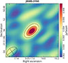 |
Fig. 1. 407 GHz dust continuum map of QSO J0305−3150 (contours at 3, 6, and 9σ). |
List of the sources analyzed in this work.
2.2. Multiwavelength data and size measurements
To perform the modified blackbody (MBB) fit, we collected additional dust continuum flux measurements at various frequencies available for the sources in our sample. These data were gathered from the specific literature and the available observations in the ALMA archive, which we reduced and analyzed using the same procedure as in the previous subsection. The complete list of flux measurements for the SED-fitting procedure is reported in Table C.1 in the appendix. Only a few corrections to our Band 8 and the published values were necessary. J0439+1634 is a strongly lensed QSO; we therefore scaled the fitted flux value down by the galaxy-integrated average magnification factor μ = 4.5 (Yue et al. 2021). A companion galaxy to PJ231−20 was instead found to be located ∼2 arcsec south of the quasar (Decarli et al. 2017). With a beam size of 4.34 × 2.92 arcsec, our observations lack the angular resolution necessary to disentangle the flux from the two galaxies. In this paper, we used as reference for the other flux measurements the data from Pensabene et al. (2021) where, however, the two sources are resolved. For this reason, we reduced and analyzed very high-resolution (with a beam size of 0.14 × 0.13 arcsec) Band 8 observations of this source from ALMA project 2022.1.00321.S (PI: Roberto Decarli), in which is possible to disentangle the quasar and the companion galaxy. We measured a flux of 8.4 ± 0.4 mJy at the observed frequency of 398 GHz for the quasar. In this map, the combined flux of the companion and QSO host agrees with the flux measured in the lower-resolution observation.
The appendix also features a size measurement of the emitting region derived from spatially resolved observations (see Table C.2), because this parameter is necessary to fit a MBB to the data. The angular extent of the emitting region Ω is computed as
 (1)
(1)
where a and b are respectively the full width at half maximum of the major and minor axis of the 2D Gaussian fit to the image plane in for spatially resolved observations. This equation corresponds to the area of an ellipse that subtends ∼98.9% of the total volume (flux) of that Gaussian. We will discuss this assumption and its impact on the fit in the following section, in light of the obtained results. For the size of QSO J0439+1439, it was necessary to convert the effective radius (re) reported by Yue et al. (2021) into the FWHM of a 2D Gaussian according to Voigt & Bridle (2010)
 (2)
(2)
where n = 1.58 is the Sérsic index and k = 1.9992n − 0.3271. For PJ083+11 instead, the angular size was computed from the physical size reported by Andika et al. (2020).
2.3. NOEMA Band 2 complementary data
In addition, we used a dedicated NOEMA program (ID: S24CH, P.I.s: Michele Costa, Leindert Boogaard) to secure dust continuum photometry of the Rayleigh-Jeans tail of the emission in PJ007+04 and PJ009−10. These observations sample the dust continuum at the observed frequency of 158 GHz, and the emission lines CO(9−8) at 1036.912 GHz, CO(10−9) at 1151.985 GHz, and H2O(32, 1–31, 2) at 1162.912 GHz rest frame. The observations and the flux of the continuum emission measured at the observed frequency of 158 GHz are summarized in Table B.1. All of them were carried out in array configuration C. The calibrated visibilities were obtained by reducing the raw data using the Grenoble Image and Line Data Analysis Software (GILDAS1). We imaged the cubes adopting a 3σ cleaning threshold, natural weighting, and a channel width of 50 km/s. To search for emission lines, we extracted the spectrum from a region centered on the brightest pixel of the continuum image, with the region size matching the clean beam. These spectra are reported in Figure B.1, along with the images of the dust emission obtained by combining the line-free channels from the two spectral windows. A continuum flux measurement was obtained from these maps with the same procedure adopted for ALMA Band 8 observations. No lines were found in the spectrum of PJ007+04, while for PJ009−10 we report a 3.4σ detection of the CO(9−8) line and a 2.4σ detection of the CO(10−9) line, obtained by fitting a Gaussian profile to the data centered at the expected transition frequency. We found a flux of  mJy km/s for the CO(9−8) line and of
  mJy km/s for the CO(10−9) line.
3. Methods and data analysis
The FIR emission of dusty astronomical objects is often modeled using multiple MBB components with different dust temperatures. In normal galaxies (see, e.g. Galametz et al. 2012), the heating of a cold dust component (Td ∼ 20 K) might be ascribed to the global starlight radiation field, which includes the contribution of evolved stars, while a warmer dust component (Td ∼ 60 K) is often associated with the emission from star-forming regions. In high-z QSOs, however, the high frequency regime in which this last component is expected to contribute most significantly is hardly accessible by current facilities. For this reason, the FIR SED of these sources is often fit using only a single dust component, even though the contribution from dust heated to higher temperatures near the SED peak is probably not negligible or might even be the primary emission source. Furthermore, in luminous QSOs, an additional hot dust component (Td > 60 K), potentially heated directly by the AGN, may dominate at rest-frame mid-infrared (MIR) wavelengths (see, e.g. Beelen et al. 2006). We carried out a spatially unresolved analysis, and assumed that the emission arises from a single dust component given by
}) \end{aligned} $$](/articles/aa/full_html/2026/02/aa56812-25/aa56812-25-eq6.gif) (3)
(3)
where νobs is the emitted frequency ν redshifted to the observer rest frame, Ω is the angular size of the emitting region, B(Td(z),ν) is the spectrum of a blackbody with temperature Td(z), B(TCMB(z),ν) is the CMB spectrum at a given redshift, and τ(ν) is the optical depth. The optical depth is defined as
 (4)
(4)
where k(ν) is the opacity, Md is the dust mass, and Ag is the physical size of the emitting region ( , with DL being the luminosity distance). Following Beelen et al. (2006) we parametrized the opacity as a power law,
 (5)
(5)
where k0 = 0.4 cm2/gr, ν0 = 250 GHz, and β is called emissivity index. To account for the effect of the dust interaction with the CMB at high redshift we followed da Cunha et al. (2013),
![Mathematical equation: $$ \begin{aligned} T_{\rm d}(z) = \left(T_{\rm d}^{4+\beta } + T_0^{4+\beta }\left[(1+z)^{4+\beta }-1\right]\right)^{1/(4+\beta )} \end{aligned} $$](/articles/aa/full_html/2026/02/aa56812-25/aa56812-25-eq10.gif) (6)
(6)
where T0 = 2.73 K is the CMB temperature at z = 0, Td(z) is the temperature of the dust at a given redshift, and Td is the intrinsic temperature of the dust at the net effect of the heating provided by the CMB. This step allowed us to compare the dust temperature in objects at different redshifts. The set of Equations (3), (4), (5) and (6) results in a full model for a source that emits as a MBB at a single temperature. We left the dust temperature, the dust mass, and the emissivity index, as free parameter and explored the 3D parameter space using a Markov chain Monte Carlo (MCMC) algorithm implemented in the EMCEE package (Foreman-Mackey et al. 2013). We assumed a uniform prior probability distribution for Td and Md in the ranges Td ∈ [1, 150] K and log Md/M⊙ ∈ [6, 10], while for β we modeled the prior probability distribution as a Gaussian with a mean value μG = 2.2 and a standard deviation σG = 0.6 (see, e.g. Bendo et al. 2025). We ran the algorithm using 45 chains, 5000 steps, and a burn-in phase of 1000 steps. In Figure 2 we show the fit SED of the QSO J0305−3150 as an example, together with the corresponding corner plots. The complete set can be found in Figure C.1 in the appendix. The SED of the QSO PJ158−14 is not shown, as the fitting algorithm did not converge because only two flux measurements were available, one in ALMA Band 8 and the other in ALMA Band 6.
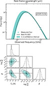 |
Fig. 2. Top panel: dust SED fit of QSO J0305−3150. Bottom panel: corner plot of the posterior probability distribution of the fit parameters. |
For each source we then computed the IR luminosity as
 (7)
(7)
where DL is the luminosity distance and S(λ) is the rest-frame specific flux emitted by the source, while for the SFR we adopted the conversion factor from Murphy et al. (2011)
 (8)
(8)
which relies on the assumption of a Kroupa initial mass function (see Kroupa & Weidner 2003). Finally, we derived the optical depths at a rest-frame frequency of 1900 GHz (τ1900) exploiting Equations (4) and (5) and the values of Md and β estimated in the fit.
4. Results
4.1. SED fit results
The physical parameters of the dust retrieved by the (converged) fits and the QSO IR luminosities, star formation rates, and optical depths at 1900 GHz are summarized in Table 2.
Infrared physical properties derived from the SED fit of the sources.
We found a mean temperature of 48 ± 3 K, which is higher than the typical dust temperatures of ∼20 K observed for main-sequence galaxies in the local universe. This result is explored in detail in the following subsection, also in view of the dust temperature evolution scenario (see, e.g. Sommovigo et al. 2022a). Interestingly, the most conspicuous outlier is QSO J0439+1634 ( K), for which the confidence value we report for the dust temperature is restricted by the upper limit of 150 K that we set as a prior in the fit (see the corresponding corner plot in Figure C.1 in the appendix). However, this source is affected by strong lensing, and the magnification factor for the central QSO derived from the Hubble Space Telescope (HST) imaging by Fan et al. (2019) has been shown to be much higher than the total magnification factor for the extended host galaxy. It is thus tempting to argue that the global temperature measured in our analysis might be enhanced due to the stronger magnification of a plausible hotter component associated with the inner regions of the QSO host. This also reflects in an extreme LIR and SFR. Therefore, J0439+1634 was not included in the plots, in the general discussion of the dust physical properties of the sample, or in the calculation of their average values.
As for dust masses, we found a mean value for log Md/M⊙ of 8.3 ± 0.1, which agrees well with the values found in Tripodi et al. (2024) for similar sources. It is of particular interest to study the relation between the gas-mass surface density ΣMd and the SFR surface density ΣSFR. We compare in Figure 3 these two physical quantities, assuming a gas-to-dust mass ratio (GDR) of 100 (see, e.g. Decarli et al. 2022; Feruglio et al. 2023). We also plot for comparison a sample of local sources from Kennicutt (1998). The strong correlation we observe (Pearson index R = 0.84, p-value p = 5 ⋅ 10−3) finds its explanation in the Kennicut-Schmidt law, while the starbursty nature of these objects seems to be linked to the low depletion time (τd < 0.01 Gyr) and not to the enhanced gas mass content, as also assessed by Kaasinen et al. (2024).
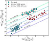 |
Fig. 3. Molecular gas-mass surface density obtained assuming a GDR = 100 vs SFR surface density. The dashed lines correspond to constant values of the gas depletion time, ranging from 1 Myr to 10 Gyr. |
Regarding dust emissivity indexes, we obtain a mean value of 2.1 ± 0.1. This parameter is directly related to the physical properties of dust grains and determines the behavior of opacity as a function of frequency (see, e.g. Draine 2003). The values we found appear to be consistent with those obtained in other studies involving similar objects (see, e.g. Witstok et al. 2023). For example, Witstok et al. (2023) found a mean value for β of 1.8 ± 0.3, without significant evolution across cosmic time, suggesting that the effective dust properties do not change dramatically with redshift. The Gaussian prior implemented in the fit also affected the derivation of this parameter little because the distribution of the derived emissivity indices exhibits a standard deviation much smaller than that of the adopted prior (0.3 and 0.6, respectively). If the derivation of β were dominated by the prior, comparable values would be expected. Its main role in the fitting procedure is to keep the uncertainties under control by discouraging the chains from exploring nonphysical values. We note that similar values for β were also obtained by Bendo et al. (2023) or in Liao et al. (2024).
Concerning infrared luminosities and star formation rates, we derive a mean value of 7.9 ± 0.9 ⋅ 1012 L⊙ and 1178 ± 140 M⊙ yr−1 respectively. These high values are justified by the construction of the sample (which selects the continuum-brightest QSOs at the rest-frame frequency of 1900 GHz) and by the high values derived for the dust temperatures. Dust emission is a thermal process (i.e., the IR radiation comes from a MBB that is in thermal equilibrium with the incident UV radiation field), and the SFRs we derived therefore probe timescales of about 100 Myr. In contrast, estimates from optical or IR lines (e.g. Hα or [OIII]88 μm) are often referred to as instantaneous SFR tracers because they are sensitive to timescales of about 10 Myr (see, e.g. Decarli et al. 2023).
Finally, the average optical depth at the rest-frame frequency of 1900 GHz for the sources in our sample is 0.26 ± 0.04. Noticeable outliers are QSOs PJ231−20 and PJ009−10 ( and
and  , respectively). The value of their optical depths is explained by the fact that these sources are either very compact (PJ231−20) or very extended (PJ009−10). At the same time, our analysis appears to point out that the widespread optically thin approximation for dust emission has to be handled with care. The high values of the emissivity index found in this sample, combined with the non-negligible optical depth at 1900 GHz, result in a rapid increase in τ(ν) with frequency, which can often exceed unity at the frequency probed by our Band 8 observations. To investigate this topic more, we plot in Figure 4 the logarithm of the dust temperature versus the logarithm of the SFR surface density ΣSFR. We then compared our data to the theoretical relation obtained by integrating Equation (3) for optically thick emission (e−τ(ν) ∼ 0) and assuming a CMB temperature TCMB(z = 6.5) = 20.5 K. This relation represents a theoretical upper limit for the sources because it traces the ΣSFR that we would obtain if these objects emitted as perfect blackbodies. The low discrepancy and the similar slope between our data and this theoretical relation suggests that the large majority of the energy emitted by the dust is radiated at frequencies where the system is optically thick, thus making the widely assumed approximation of optically thin emission questionable for this type of sources. QSO PJ009−10 is interestingly the most distant object from this theoretical relation because its relatively extended shape causes a lower optical depth than for the other sources. In contrast, the closest object is PJ231−20, which has the most compact sizes and therefore the highest value of τ1900.
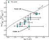 |
Fig. 4. Dust temperature vs SFR surface density. The dashed black line corresponds to the relation obtained by analytically integrating Equation (3) under optically thick conditions and assuming a z = 6.5 background CMB radiation field. The two sources indicated by the arrows are PJ009−10 and PJ231−20, which show the lowest and highest value of τ1900, respectively. |
Given that the compact size of the objects appears to be the primary driver of their optical thickness, and considering that our fits rely entirely on a single size measurement from ALMA Band 6, we decided to investigate the effect of a changed definition of the angular size of the source Ω on our results. In Figure 5 we plot the ratios Td/Td, thin and log Md/log Md, thin as a function of the assumed source size expressed in units of σ of the fitted Gaussian (Rσ). The subscript thin refers to the quantities derived by running the fit again under the optically thin MBB emission approximation of Equation (3)
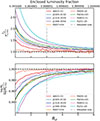 |
Fig. 5. Median values of the Td and Md posterior probability distribution as functions of the assumed size, normalized to the optically thin results. The dashed line marks the asymptotic limit of 1 expected for low optical depth. The upper x-axis shows the fractional luminosity enclosed within the corresponding σ distance from the Gaussian peak. |
![Mathematical equation: $$ \begin{aligned} S(\nu _{\rm obs})_{\rm thin} = \dfrac{(1+z)}{D_{\rm L}^{2}}[B(T_{\rm d}(z),\nu )-B(T_{\rm CMB}(z),\nu )]\cdot k(\nu )M_{\rm d}. \end{aligned} $$](/articles/aa/full_html/2026/02/aa56812-25/aa56812-25-eq76.gif) (9)
(9)
Under this assumption, this equation loses the dependence on the solid angle Ω, so at high-z it is often used when spatially resolved observations are not available. We recall that in our general analysis, we defined the source size as an ellipse encompassing 98.9% (3σ) of the total flux (volume) of the Gaussian. These plots show that, as expected, increasing the assumed size causes the quantities derived in the general case to asymptotically approach those obtained under the optically thin approximation. This is because the progressively lower optical depth increasingly justifies the optically thin assumption. This is also noticeable in the case of PJ009−10, for which the optically thin case appears to yield reliable results. Additionally, this approximation systematically underestimates the dust temperature and overestimates the dust mass, both by approximately 40%. In contrast, the emissivity index, although it still converges to βthin at high values of Rσ, displays no clear trend as the assumed size increases, and therefore we did not not include it in Figure 5.
4.2. Dust temperature in QSOs and galaxies across redshift
As mentioned in the previous section, the dust temperature of the in our sample ranged from 34 K to 65 K, which is higher than the temperatures derived for local, main-sequence galaxies. An evolution with redshift of this quantity in UV-selected star-forming galaxies as recently been suggested (see, e.g. Schreiber et al. 2018; Bouwens et al. 2020; Faisst et al. 2020; Ismail et al. 2023). However, while the studies agreed on the existence of the trend, the descriptions of its behavior at redshift higher than 4 vary widely. For example, Bouwens et al. (2020) reported that z and Td can be linked by a linear relation up to z ≃ 7.5, while Faisst et al. (2020) found that the relation seems to flatten at z > 4. While neither behavior was not fully explained by a complete physical model so far, theoretical works suggested that the increase oin the dust temperature with redshift might be related to the higher values of the sSFR or of the SFE in galaxies at high-z (see, e.g. Shen et al. 2022; Sommovigo et al. 2022a), which may translate into a dust distribution that is more concentrated in star-forming regions (see, e.g. Liang et al. 2019).
However, when only luminous, ultraluminous, and hyperluminous infrared galaxies (LIRGs, ULIRGs, and HLIRGs, respectively) are taken into consideration, the infrared luminosities of which are comparable to the ones of the quasar hosts in our sample, the picture is different. Figure 6, shows the dust temperature versus redshift for the sources we analyzed in this work and a sample of IR-luminous starburst galaxies selected to have LIR > 1011 L⊙. For this galaxy sample the dust temperature appears to remain constant across all redshifts, while also being comparable to the values derived for the QSO hosts in this study. This might seem like a trivial result, as we selected these galaxies because of their high IR luminosities, and we discussed above that Td is an important driver of LIR. The evolution of the dust temperature still lacks survey-like studies capable of accounting for observational biases that favor the selection of UV-brighter systems, however, which may exhibit hotter dust due to increased UV absorption and grain reprocessing, or even colder dust, if these objects appear UV bright because the radiation in these systems is less attenuated (and thus less reprocessed) by dust grains.
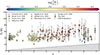 |
Fig. 6. Dust temperature versus redshift in a sample of LIRGs, ULIRGs and HLIRGs, and in our QSOs. The dashed area corresponds to the CMB temperature. Data from Yang et al. (2007), Younger et al. (2009), Magdis et al. (2010), Clements et al. (2018), Franco et al. (2020), Reuter et al. (2020), Witstok et al. (2023), Mitsuhashi et al. (2024). |
Despite this limitation, Sommovigo et al. (2022b,a) attempted to extend the study of the dust temperature across cosmic time by including single-band Td estimates that exploited the [CII]158 μm line luminosity and the underlying continuum flux for ALPINE and REBELS galaxies. They obtained an average value of Td = 48 ± 2 K and Td = 47 ± 2 K respectively. The objects targeted by these programs are mostly main-sequence galaxies, which nevertheless show higher Td than their local counterparts. This effect is likely linked to the evolution of the M*–SFR main sequence itself, as also discussed by Schreiber et al. (2018), which makes these galaxies progressively more similar to those we plot in Figure 6 as redshift increases. It is of particular interest that the Td they derived is not different to the one of 6 < z < 7 QSO hosts. This suggests that the processes that heat the dust are similar in all of these objects.
4.3. The [CII]158 μm deficit
For sources with a high IR luminosity as the one presented here, several works (see, e.g., Díaz-Santos et al. 2013, 2017; Decarli et al. 2018) have found that multiple FIR fine-structure lines, such as the [CII]158 μm, [NII]122 μm or the [OI]63 μm show a decrease, or deficit, in the ratio of their luminosity and the IR luminosity of the source as this last quantity increases. While the physical motivation of this phenomenon can not be ascribed to a single factor, one possible explanation was suggested to be a different spatial distribution of dust, with it being more concentrated inside the star-forming regions in higher-luminosity systems (see, e.g. Díaz-Santos et al. 2013). In this scenario, a larger fraction of UV photons emitted by stars is absorbed by dust within the HII region, efficiently heating the dust grains while simultaneously reducing the UV photon flux that reaches the photodissociation region (PDR). This leads to a deficit in photoelectrons produced by the ionization of polycyclic aromatic hydrocarbons (PAHs) and dust grains, thus affecting the emission of lines such as [CII]158 μm. This combination of effects can enhance the infrared luminosity emitted by the dust and suppress the [CII]158 μm line emission. The former of the two processes would also explain why the observed line deficits concern lines that trace different ISM phases, or which emission integrated along the line of sight includes contributions from more than one of these phases (see, e.g. Croxall et al. 2017; Ramos Padilla et al. 2023).
In Figure 7 we plot the ratio of [CII]158 μm to FIR luminosity against dust temperature for a sample of local IR galaxies from Díaz-Santos et al. (2017) and the QSOs in this work. This provides a direct link between the previously described scenario and the physical origin of the [CII]158 μm line deficit, with high dust temperature tracing the compact, dust-bounded nature of the star-forming regions responsible for the enhanced IR luminosity. While it is true that, for fixed values of Md, GDR, and physical properties of the [CII]158 μm-emitting gas, a higher Td leads to a more pronounced [CII]158 μm deficit by definition, it is important to point out that the physical conditions of the gas are not independent of Td. Several studies have shown that the dust temperature correlates with the kinetic temperature of the [CII] colliders (typically electrons in ionized regions and neutral atoms or H2 molecules in denser phases; see, Zhao et al. 2024 for an example), hence altering the excitation temperature of [CII]. This coupling can enhance the line emissivity and thereby partly compensate for the [CII]158 μm deficit. The behavior of our QSOs appears to agree with the empirical trend fit in Díaz-Santos et al. (2017), especially for lower values of Td, while for higher dust temperatures, these source effectively probe a regime that was previously not accessed.
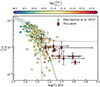 |
Fig. 7. [CII]158 μm line luminosity deficit as function of dust temperature for the sample of Díaz-Santos et al. (2017) and for the QSOs of this work. In the former sample the dust temperature is derived by the color index S63 μm/S158 μm, assuming MBB optically thin emission with β = 1.8. The dashed black line is the best fit from Díaz-Santos et al. (2017), and the two dashed lines represent the 1σ scatter from this relation. |
4.4. Contribution of the central AGN to the surrounding dust heating
It is possible to argue that the presence of a very bright active galactic nucleus may heat the innermost-located dust of the host galaxy, the emission of which could contaminate our unresolved Band 8 flux measurements. This raises the concern that the values obtained from the SED fitting for this quantity do not accurately represent the value at which the dust grains in the host are at thermodynamical equilibrium, leaving open the possibility that the temperature estimates in our sources could be biased. A temperature gradient that peaks in the galaxy center has been hinted by the results obtained for the lensed QSO J0439−1634. However, the contribution of this gradient to the rest of the sample remains unconstrained.
Nevertheless, Figure 6 shows that the QSOs of this work appear to follow the trend in dust temperature against redshift that is observed in LIRGs, ULIRGs, and HLIRGs, which is not expected for the case of AGN contamination. Additionally, given that 407 GHz observations do not seem to probe frequencies higher than the emission peak and that a single-temperature MBB seems to fit the observed SED in most of the sources well, the measured contribution of the AGN-heated dust component may be negligible (see also Sommovigo & Algera 2025). To fully determine the role that this factor plays in the dust properties derived here, high-resolution ALMA Band 9 or Band 10 observations are needed, however. These would be able to sample the SED in the rest-frame mid-infrared (MIR) band, where an eventual central hot dust (Td > 60 K) is expected to peak, and to disentangle it from the more diffused emission of the galaxy. Unfortunately, these type of data are available for very few sources so far. For example, Tsukui et al. (2023) fit a MBB law to the observed emission of a QSO at z = 4.4 by decomposing it into a galaxy-scale component and a component originating from the innermost resolution beam (effective radius of 720 pc). They reported a temperature of the cold dust component (associated with the galaxy-scale emission) of  K, and of
  K for the hot component (which is associated to AGN-heated dust, with a possible contribution from the dusty torus). Meyer et al. (2025) analyzed the source J2348−3054 based on new spatially resolved observation, which revealed a steep gradient in Td that peaked at
  K in the innermost region of 216 pc radius. When they include a torus model, however, this value is slightly reduced to
  K, suggesting the presence of a component of hot dust heated by AGN radiation that is physically distinct from the torus. Dust-temperature gradients at high redshift have also been observed in galaxies that do not host an AGN. Akins et al. (2022), for example, fit the FIR emission of A1689-zD1, a strongly lensed ULIRG at z = 7.13 with a magnification factor of μ = 9.3, which remained nearly constant across the entire spatial extent of the source (∼7 kpc). They reported a galaxy-averaged dust temperature of
  K, while the temperature reached approximately 50 K in central 900 pc. Both values are consistent within the uncertainties with the average dust temperatures derived in this work for QSO host galaxies. In this context, the temperature gradient in A1689-zD1 likely reflects a higher fraction of dust heated by intense central star formation.
5. Conclusions
We presented a sample of 11 QSO host galaxies for which we had new ALMA ACA Band 8 observations. For 10 of them we were able to constrain their interstellar dust physical properties, infrared luminosities and star formation rates. The main results are summarized below.
-
The SED fitting of all the IR emission of the sources confirmed the extreme starbursty nature of QSOs host galaxies, which is likely driven by the short gas depletion times.
-
The high value of their optical depths at 1900 GHz, as well as the behavior of their ΣSFR as function of Td, revealed that the large majority of their energy is radiated at frequencies at which the system is optically thick. This discourages the use of the commonly assumed optically thin approximation when their IR emission is fit.
-
The values of the dust temperature we derived agree quite well with the temperature found for LIRGs, ULIRGs, and HLIRGs across different cosmic times. The physical explanation of this is likely to be found in the short depletion times (high SFEs) that these sources were already confirmed to have. This scenario is consistent with a larger fraction of dust being situated in SF regions with respect to local star-forming galaxies.
-
The dusty nature of SF region also appears to be confirmed by the link between the [CII]158 μm deficit and the dust temperature, with our QSOs sampling a regime that was previously not probed.
-
We found no strong evidence that the AGN affects the results obtained by the unresolved SED fit, but to fully assess the role it plays in the energetic of the dust emission further high-frequency, high-resolution ALMA observations are needed.
Acknowledgments
M.C., R.D., and F.X. acknowledge support from the INAF GO grant 2022 “The birth of the giants: JWST sheds light on the build-up of quasars at cosmic dawn”, INAF Minigrant 2024 “The interstellar medium at high redshift”, and by the PRIN MUR “2022935STW”, RFF M4.C2.1.1, CUP J53D23001570006 and C53D23000950006. R.A.M. acknowledges support from the Swiss National Science Foundation (SNSF) through project grant 200020_207349. A.P. acknowledges the support from the Fondazione Cariplo grant “2020-0902”. This paper makes use of the following ALMA data: ADS/JAO.ALMA#2019.2.00053.S, ADS/JAO.ALMA#2019.1.00147.S, ADS/JAO.ALMA#2021.2.00064.S, ADS/JAO.ALMA#2021.2.00151.S, ADS/JAO.ALMA#2022.1.00321.S, ADS/JAO.ALMA#2023.1.01450.S, and ADS/JAO.ALMA#2024.1.00071.S. ALMA is a partnership of ESO (representing its member states), NSF (USA) and NINS (Japan), together with NRC (Canada), NSTC and ASIAA (Taiwan), and KASI (Republic of Korea), in cooperation with the Republic of Chile. The Joint ALMA Observatory is operated by ESO, AUI/NRAO and NAOJ. This work is based on observations carried out under project number S24CH with the IRAM NOEMA Interferometer. IRAM is supported by INSU/CNRS (France), MPG (Germany) and IGN (Spain).
References
- Akins, H. B., Fujimoto, S., Finlator, K., et al. 2022, ApJ, 934, 64 [NASA ADS] [CrossRef] [Google Scholar]
- Andika, I. T., Jahnke, K., Onoue, M., et al. 2020, ApJ, 903, 34 [Google Scholar]
- Ansarinejad, B., Shanks, T., Bielby, R. M., et al. 2022, MNRAS, 510, 4976 [Google Scholar]
- Beelen, A., Cox, P., Benford, D. J., et al. 2006, ApJ, 642, 694 [NASA ADS] [CrossRef] [Google Scholar]
- Bendo, G. J., Urquhart, S. A., Serjeant, S., et al. 2023, MNRAS, 522, 2995 [NASA ADS] [CrossRef] [Google Scholar]
- Bendo, G. J., Bakx, T. J. L. C., Algera, H. S. B., et al. 2025, MNRAS, 540, 1560 [Google Scholar]
- Bouwens, R., González-López, J., Aravena, M., et al. 2020, ApJ, 902, 112 [NASA ADS] [CrossRef] [Google Scholar]
- Butler, K. M., van der Werf, P. P., Topkaras, T., et al. 2023, ApJ, 944, 134 [NASA ADS] [CrossRef] [Google Scholar]
- Carnall, A. C., McLure, R. J., Dunlop, J. S., et al. 2023, Nature, 619, 716 [NASA ADS] [CrossRef] [Google Scholar]
- CASA Team (Bean, B., et al.) 2022, PASP, 134, 114501 [NASA ADS] [CrossRef] [Google Scholar]
- Cimatti, A., Daddi, E., & Renzini, A. 2006, A&A, 453, L29 [NASA ADS] [CrossRef] [EDP Sciences] [Google Scholar]
- Clements, D. L., Pearson, C., Farrah, D., et al. 2018, MNRAS, 475, 2097 [NASA ADS] [CrossRef] [Google Scholar]
- Croxall, K. V., Smith, J. D., Pellegrini, E., et al. 2017, ApJ, 845, 96 [Google Scholar]
- da Cunha, E., Groves, B., Walter, F., et al. 2013, ApJ, 766, 13 [Google Scholar]
- Decarli, R., Walter, F., Venemans, B. P., et al. 2017, Nature, 545, 457 [Google Scholar]
- Decarli, R., Walter, F., Venemans, B. P., et al. 2018, ApJ, 854, 97 [Google Scholar]
- Decarli, R., Pensabene, A., Venemans, B., et al. 2022, A&A, 662, A60 [NASA ADS] [CrossRef] [EDP Sciences] [Google Scholar]
- Decarli, R., Pensabene, A., Diaz-Santos, T., et al. 2023, A&A, 673, A157 [NASA ADS] [CrossRef] [EDP Sciences] [Google Scholar]
- Díaz-Santos, T., Armus, L., Charmandaris, V., et al. 2013, ApJ, 774, 68 [Google Scholar]
- Díaz-Santos, T., Armus, L., Charmandaris, V., et al. 2017, ApJ, 846, 32 [Google Scholar]
- Ding, X., Silverman, J. D., & Onoue, M. 2022, ApJ, 939, L28 [NASA ADS] [CrossRef] [Google Scholar]
- Draine, B. T. 2003, ARA&A, 41, 241 [NASA ADS] [CrossRef] [Google Scholar]
- Eilers, A.-C., Hennawi, J. F., Decarli, R., et al. 2020, ApJ, 900, 37 [Google Scholar]
- Elia, D., & Pezzuto, S. 2016, MNRAS, 461, 1328 [Google Scholar]
- Faisst, A. L., Fudamoto, Y., Oesch, P. A., et al. 2020, MNRAS, 498, 4192 [NASA ADS] [CrossRef] [Google Scholar]
- Fan, X., Wang, F., Yang, J., et al. 2019, ApJ, 870, L11 [Google Scholar]
- Farina, E. P., Schindler, J.-T., Walter, F., et al. 2022, ApJ, 941, 106 [NASA ADS] [CrossRef] [Google Scholar]
- Feruglio, C., Maio, U., Tripodi, R., et al. 2023, ApJ, 954, L10 [NASA ADS] [CrossRef] [Google Scholar]
- Foreman-Mackey, D., Hogg, D. W., Lang, D., & Goodman, J. 2013, PASP, 125, 306 [Google Scholar]
- Franco, M., Elbaz, D., Zhou, L., et al. 2020, A&A, 643, A30 [NASA ADS] [CrossRef] [EDP Sciences] [Google Scholar]
- Galametz, M., Kennicutt, R. C., Albrecht, M., et al. 2012, MNRAS, 425, 763 [NASA ADS] [CrossRef] [Google Scholar]
- Gilli, R., Norman, C., Calura, F., et al. 2022, A&A, 666, A17 [NASA ADS] [CrossRef] [EDP Sciences] [Google Scholar]
- Hopkins, P. F., Hernquist, L., Cox, T. J., & Kereš, D. 2008, ApJS, 175, 356 [Google Scholar]
- Inami, H., Algera, H. S. B., Schouws, S., et al. 2022, MNRAS, 515, 3126 [NASA ADS] [CrossRef] [Google Scholar]
- Ismail, D., Beelen, A., Buat, V., et al. 2023, A&A, 678, A27 [Google Scholar]
- Kaasinen, M., Venemans, B., Harrington, K. C., et al. 2024, A&A, 684, A33 [NASA ADS] [CrossRef] [EDP Sciences] [Google Scholar]
- Kennicutt, R. C. 1998, ApJ, 498, 541 [NASA ADS] [CrossRef] [Google Scholar]
- Kroupa, P., & Weidner, C. 2003, ApJ, 598, 1076 [NASA ADS] [CrossRef] [Google Scholar]
- Liang, L., Feldmann, R., Kereš, D., et al. 2019, MNRAS, 489, 1397 [NASA ADS] [CrossRef] [Google Scholar]
- Liao, C.-L., Chen, C.-C., Wang, W.-H., et al. 2024, ApJ, 961, 226 [NASA ADS] [CrossRef] [Google Scholar]
- Ma, X., Hayward, C. C., Casey, C. M., et al. 2019, MNRAS, 487, 1844 [NASA ADS] [CrossRef] [Google Scholar]
- Magdis, G. E., Elbaz, D., Hwang, H. S., et al. 2010, MNRAS, 409, 22 [NASA ADS] [CrossRef] [Google Scholar]
- Meyer, R. A., Walter, F., Di Mascia, F., et al. 2025, A&A, 695, L18 [NASA ADS] [CrossRef] [EDP Sciences] [Google Scholar]
- Mitsuhashi, I., Harikane, Y., Bauer, F. E., et al. 2024, ApJ, 971, 161 [NASA ADS] [CrossRef] [Google Scholar]
- Murphy, E. J., Condon, J. J., Schinnerer, E., et al. 2011, ApJ, 737, 67 [Google Scholar]
- Neeleman, M., Novak, M., Venemans, B. P., et al. 2021, ApJ, 911, 141 [NASA ADS] [CrossRef] [Google Scholar]
- Novak, M., Bañados, E., Decarli, R., et al. 2019, ApJ, 881, 63 [NASA ADS] [CrossRef] [Google Scholar]
- Pensabene, A., Decarli, R., Bañados, E., et al. 2021, A&A, 652, A66 [NASA ADS] [CrossRef] [EDP Sciences] [Google Scholar]
- Planck Collaboration VI. 2020, A&A, 641, A6 [NASA ADS] [CrossRef] [EDP Sciences] [Google Scholar]
- Ramos Padilla, A. F., Wang, L., van der Tak, F. F. S., & Trager, S. C. 2023, A&A, 679, A131 [NASA ADS] [CrossRef] [EDP Sciences] [Google Scholar]
- Renzini, A. 2006, ARA&A, 44, 141 [NASA ADS] [CrossRef] [Google Scholar]
- Reuter, C., Vieira, J. D., Spilker, J. S., et al. 2020, ApJ, 902, 78 [NASA ADS] [CrossRef] [Google Scholar]
- Schreiber, C., Elbaz, D., Pannella, M., et al. 2018, A&A, 609, A30 [NASA ADS] [CrossRef] [EDP Sciences] [Google Scholar]
- Shen, X., Vogelsberger, M., Nelson, D., et al. 2022, MNRAS, 510, 5560 [NASA ADS] [CrossRef] [Google Scholar]
- Somerville, R. S., & Davé, R. 2015, ARA&A, 53, 51 [Google Scholar]
- Sommovigo, L., & Algera, H. 2025, MNRAS, 540, 3693 [Google Scholar]
- Sommovigo, L., Ferrara, A., Pallottini, A., et al. 2022a, MNRAS, 513, 3122 [NASA ADS] [CrossRef] [Google Scholar]
- Sommovigo, L., Ferrara, A., Carniani, S., et al. 2022b, MNRAS, 517, 5930 [NASA ADS] [CrossRef] [Google Scholar]
- Spilker, J. S., Champagne, J. B., Fan, X., et al. 2025, ApJ, 982, 72 [Google Scholar]
- Symeonidis, M., & Page, M. J. 2021, MNRAS, 503, 3992 [NASA ADS] [CrossRef] [Google Scholar]
- Thomas, M. O., Shemmer, O., Trakhtenbrot, B., et al. 2023, ApJ, 955, 15 [NASA ADS] [CrossRef] [Google Scholar]
- Tripodi, R., Feruglio, C., Fiore, F., et al. 2022, A&A, 665, A107 [NASA ADS] [CrossRef] [EDP Sciences] [Google Scholar]
- Tripodi, R., Feruglio, C., Fiore, F., et al. 2024, A&A, 689, A220 [NASA ADS] [CrossRef] [EDP Sciences] [Google Scholar]
- Tsukui, T., Wisnioski, E., Krumholz, M. R., & Battisti, A. 2023, MNRAS, 523, 4654 [NASA ADS] [CrossRef] [Google Scholar]
- Venemans, B. P., Walter, F., Decarli, R., et al. 2017, ApJ, 845, 154 [Google Scholar]
- Venemans, B. P., Decarli, R., Walter, F., et al. 2018, ApJ, 866, 159 [Google Scholar]
- Venemans, B. P., Walter, F., Neeleman, M., et al. 2020, ApJ, 904, 130 [Google Scholar]
- Voigt, L. M., & Bridle, S. L. 2010, MNRAS, 404, 458 [Google Scholar]
- Wang, F., Yang, J., Fan, X., et al. 2024, ApJ, 968, 9 [NASA ADS] [CrossRef] [Google Scholar]
- Witstok, J., Jones, G. C., Maiolino, R., Smit, R., & Schneider, R. 2023, MNRAS, 523, 3119 [NASA ADS] [CrossRef] [Google Scholar]
- Yang, M., Greve, T. R., Dowell, C. D., & Borys, C. 2007, ApJ, 660, 1198 [NASA ADS] [CrossRef] [Google Scholar]
- Yang, J., Venemans, B., Wang, F., et al. 2019, ApJ, 880, 153 [NASA ADS] [CrossRef] [Google Scholar]
- Younger, J. D., Omont, A., Fiolet, N., et al. 2009, MNRAS, 394, 1685 [Google Scholar]
- Yue, M., Yang, J., Fan, X., et al. 2021, ApJ, 917, 99 [NASA ADS] [CrossRef] [Google Scholar]
- Zhao, X., Tang, X. D., Henkel, C., et al. 2024, A&A, 687, A207 [NASA ADS] [CrossRef] [EDP Sciences] [Google Scholar]
Appendix A: ALMA Band 8 observations
Characteristics of the ALMA Band 8 observations analyzed in this work.
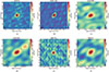 |
Fig. A.1. 407 GHz dust continuum maps for the sources analyzed in this work. The clean beam is reported in the bottom left corner of each panel. Panel (a): QSO AJ025-33 (contours at 3, 9, 15, 21 and 27 σ). Panel (b): QSO J0439+1634 (contours at 3, 9, 15, 21 and 27 σ). Panel (c): QSO J2318-3029 (contours at 3, 6 and 9 σ). Panel (d): QSO J2348-3054 (contours at 3, 6, 9 and 12 σ). Panel (e): QSO PJ007+04 (contours at 3, 9 and 15 σ). Panel (f): QSO PJ009-10 (contours at 3, 6 and 9 σ). Panel (g): QSO PJ036+03 (contours at 3, 9 and 15 σ). Panel (h): QSO PJ083+11 (contours at 3, 6, 9 and 12 σ). Panel (i): QSO PJ158-14 (contours at 3, 9 and 15 σ). Panel (j): QSO PJ231-20 (contours at 3, 6 and 9 σ). |
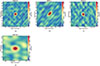 |
Fig. A.1. continued. |
Appendix B: NOEMA Band 2 observations
Characteristics of the NOEMA Band 2 observations analyzed in this work.
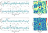 |
Fig. B.1. NOEMA Band 2 spectra and dust continuum maps for the QSOs PJ007+04 and PJ009-10. The clean beam is reported in the bottom left corner of each continuum map. Panel (a): spectrum of the QSO PJ007+04 extracted over a region corresponding to the clean beam, with channel widths of 50 km/s. The light blue curve represents the fitted model, consisting of a constant continuuum and, in case of detection, some Gaussian line components. Panel (b): 158 GHz dust continuum map of the QSO PJ007+04 (contours at 3, 6 and 9 σ). Panel (c): same as panel (a) but for the QSO PJ009-10. Panel (d): same as panel (b) but for the QSO PJ009-10 (contours at 3, 9, 15, 21 and 27 σ). |
Appendix C: SED fitting
Data used to fit the SEDs.
Spatial extent of the sources analyzed in this work.
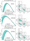 |
Fig. C.1. Left panels: fits of the IR-SED of the QSOs in this sample. Right panels: corner plots of the parameters’ posterior probability distribution. We only report the sources for which the algorithm converged |
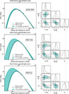 |
Fig. C.1. continued. |
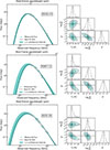 |
Fig. C.1. continued. |
All Tables
All Figures
|
Fig. 1. 407 GHz dust continuum map of QSO J0305−3150 (contours at 3, 6, and 9σ). |
| In the text | |
|
Fig. 2. Top panel: dust SED fit of QSO J0305−3150. Bottom panel: corner plot of the posterior probability distribution of the fit parameters. |
| In the text | |
|
Fig. 3. Molecular gas-mass surface density obtained assuming a GDR = 100 vs SFR surface density. The dashed lines correspond to constant values of the gas depletion time, ranging from 1 Myr to 10 Gyr. |
| In the text | |
|
Fig. 4. Dust temperature vs SFR surface density. The dashed black line corresponds to the relation obtained by analytically integrating Equation (3) under optically thick conditions and assuming a z = 6.5 background CMB radiation field. The two sources indicated by the arrows are PJ009−10 and PJ231−20, which show the lowest and highest value of τ1900, respectively. |
| In the text | |
|
Fig. 5. Median values of the Td and Md posterior probability distribution as functions of the assumed size, normalized to the optically thin results. The dashed line marks the asymptotic limit of 1 expected for low optical depth. The upper x-axis shows the fractional luminosity enclosed within the corresponding σ distance from the Gaussian peak. |
| In the text | |
|
Fig. 6. Dust temperature versus redshift in a sample of LIRGs, ULIRGs and HLIRGs, and in our QSOs. The dashed area corresponds to the CMB temperature. Data from Yang et al. (2007), Younger et al. (2009), Magdis et al. (2010), Clements et al. (2018), Franco et al. (2020), Reuter et al. (2020), Witstok et al. (2023), Mitsuhashi et al. (2024). |
| In the text | |
|
Fig. 7. [CII]158 μm line luminosity deficit as function of dust temperature for the sample of Díaz-Santos et al. (2017) and for the QSOs of this work. In the former sample the dust temperature is derived by the color index S63 μm/S158 μm, assuming MBB optically thin emission with β = 1.8. The dashed black line is the best fit from Díaz-Santos et al. (2017), and the two dashed lines represent the 1σ scatter from this relation. |
| In the text | |
|
Fig. A.1. 407 GHz dust continuum maps for the sources analyzed in this work. The clean beam is reported in the bottom left corner of each panel. Panel (a): QSO AJ025-33 (contours at 3, 9, 15, 21 and 27 σ). Panel (b): QSO J0439+1634 (contours at 3, 9, 15, 21 and 27 σ). Panel (c): QSO J2318-3029 (contours at 3, 6 and 9 σ). Panel (d): QSO J2348-3054 (contours at 3, 6, 9 and 12 σ). Panel (e): QSO PJ007+04 (contours at 3, 9 and 15 σ). Panel (f): QSO PJ009-10 (contours at 3, 6 and 9 σ). Panel (g): QSO PJ036+03 (contours at 3, 9 and 15 σ). Panel (h): QSO PJ083+11 (contours at 3, 6, 9 and 12 σ). Panel (i): QSO PJ158-14 (contours at 3, 9 and 15 σ). Panel (j): QSO PJ231-20 (contours at 3, 6 and 9 σ). |
| In the text | |
|
Fig. A.1. continued. |
| In the text | |
|
Fig. B.1. NOEMA Band 2 spectra and dust continuum maps for the QSOs PJ007+04 and PJ009-10. The clean beam is reported in the bottom left corner of each continuum map. Panel (a): spectrum of the QSO PJ007+04 extracted over a region corresponding to the clean beam, with channel widths of 50 km/s. The light blue curve represents the fitted model, consisting of a constant continuuum and, in case of detection, some Gaussian line components. Panel (b): 158 GHz dust continuum map of the QSO PJ007+04 (contours at 3, 6 and 9 σ). Panel (c): same as panel (a) but for the QSO PJ009-10. Panel (d): same as panel (b) but for the QSO PJ009-10 (contours at 3, 9, 15, 21 and 27 σ). |
| In the text | |
|
Fig. C.1. Left panels: fits of the IR-SED of the QSOs in this sample. Right panels: corner plots of the parameters’ posterior probability distribution. We only report the sources for which the algorithm converged |
| In the text | |
|
Fig. C.1. continued. |
| In the text | |
|
Fig. C.1. continued. |
| In the text | |
Current usage metrics show cumulative count of Article Views (full-text article views including HTML views, PDF and ePub downloads, according to the available data) and Abstracts Views on Vision4Press platform.
Data correspond to usage on the plateform after 2015. The current usage metrics is available 48-96 hours after online publication and is updated daily on week days.
Initial download of the metrics may take a while.