| Issue |
A&A
Volume 706, February 2026
|
|
|---|---|---|
| Article Number | A272 | |
| Number of page(s) | 19 | |
| Section | Interstellar and circumstellar matter | |
| DOI | https://doi.org/10.1051/0004-6361/202556867 | |
| Published online | 17 February 2026 | |
Chemical study of two starless cores in the B213/L1495 filament
1
Centro de Astrobiología (CSIC-INTA),
Ctra. de Ajalvir, km 4, Torrejón de Ardoz,
28850
Madrid,
Spain
2
European Space Agency (ESA), European Space Astronomy Centre (ESAC),
Camino Bajo del Castillo s/n,
28692
Villanueva de la Cañada,
Madrid,
Spain
3
Observatorio Astronómico Nacional (OAN),
Alfonso XII, 3,
28014
Madrid,
Spain
4
Observatorio de Yebes (IGN),
Cerro de la Palera s/n,
19141
Yebes,
Guadalajara,
Spain
5
Instituto de Astrofísica de Canarias (IAC),
Avda Vía Láctea s/n,
38200
La Laguna,
Tenerife,
Spain
6
Departamento de Astrofísica, Universidad de La Laguna,
38205
La Laguna,
Tenerife,
Spain
★ Corresponding author: This email address is being protected from spambots. You need JavaScript enabled to view it.
Received:
14
August
2025
Accepted:
28
November
2025
Abstract
Context. The chemical evolution of pre-stellar cores during their transition to a protostellar stage is not yet fully understood. Detailed chemical characterizations of these sources are needed to better define their chemistry during star formation.
Aims. Our goal is to characterize the chemistry of the starless cores C2 and C16 in the B213/L1495 filament of the Taurus Molecular Cloud, and to understand how it relates to the environmental conditions and the evolutionary state of the cores.
Methods. We made use of two complete spectral surveys at 7 mm of these sources, carried out using the Yebes 40-m telescope. Derived molecular abundances were compared with those of other sources in different evolutionary stages and with values computed by chemical models.
Results. Including isotopologs, 22 molecules were detected in B213-C2, and 25 in B213-C16. The derived rotational temperatures have values of between ∼5 K and ∼9 K. A comparison of the two sources shows lower abundances in C2, except for l-C3H and HOCO+, which have similar values in both cores. Model results indicate that both cores are best fit assuming early-time chemistry, and point to C2 being in a more advanced evolutionary stage, as it presents a higher molecular hydrogen density and sulfur depletion, and a lower cosmic-ray ionization rate. Our chemical modeling successfully accounts for the abundances of most molecules, including complex organic molecules and long cyanopolynes (HC5N, HC7N), but fails to reproduce those of the carbon chains CCS and C3O.
Conclusions. Chemical differences between C2 and C16 could stem from the evolutionary stage of the cores, with C2 being closer to the pre-stellar phase. Both cores are better fit assuming early-time chemistry of t ~ 0.1 Myr. The more intense UV radiation in the northern region of B213 could account for the high abundances of l-C3H and HOCO+ in C2.
Key words: astrochemistry / line: identification / stars: formation / stars: low-mass / ISM: abundances / ISM: molecules
© The Authors 2026
 Open Access article, published by EDP Sciences, under the terms of the Creative Commons Attribution License (https://creativecommons.org/licenses/by/4.0), which permits unrestricted use, distribution, and reproduction in any medium, provided the original work is properly cited.
This article is published in open access under the Subscribe to Open model. This email address is being protected from spambots. You need JavaScript enabled to view it. to support open access publication.
1 Introduction
The Herschel Space Telescope has transformed our understanding of star-forming regions. Images of giant molecular clouds and dark cloud complexes have revealed spectacular networks of filamentary structures where stars are born (André et al. 2010). Now we think that interstellar filaments are present throughout the Milky Way and are the preferred sites for star formation. These filaments funnel interstellar gas and dust into increasingly dense concentrations. These concentrations then contract and fragment, leading to gravitationally bound pre-stellar cores that will eventually form stars (André et al. 2010; Molinari et al. 2010; Juvela et al. 2012).
Gas chemistry plays a pivotal role in the process of star formation by regulating critical processes, such as gas cooling and the ionization fraction. Molecular filaments have been observed to fragment into dense cores due to the cooling of the gas by molecules (Goldsmith & Langer 1978), thereby reducing the thermal support relative to self-gravity. The ionization fraction exerts a critical influence on the coupling of magnetic fields with the gas, thereby driving the dissipation of turbulence and angular momentum transfer. Consequently, it plays a crucial role in the cloud collapse (isolated vs. clustered star formation) and the dynamics of accretion discs (see Padovani et al. 2013; Zhao et al. 2021). The gas ionization fraction and molecular abundances are contingent upon the elemental depletion factors, as was demonstrated in Caselli et al. (1998). In particular, carbon (C) is the primary electron donor in the cloud surface (Av < 4 mag), and sulfur (S) is the primary donor in the range of AV = 3.7-7 magnitudes, which encompasses a significant fraction of the molecular cloud mass, given its lower ionization potential and its status as a non-depleted element (Goicoechea et al. 2006). Therefore, sulfur depletion constitutes a valuable piece of information for our understanding of the grain composition and evolution.
Dense cores set the initial conditions for the process of star formation (see, e.g., Shu et al. 1987; Bergin & Tafalla 2007). Gas and solids undergo a continuous evolution from their early stages in molecular clouds to their incorporation into a growing planet through a proto-planetary disk. Although this evolution takes place over the course of several million years, it is now believed that the chemical composition of the disk is largely influenced by the physical and chemical conditions present in the progenitor molecular cloud (Visser et al. 2009; Öberg et al. 2011; Navarro-Almaida et al. 2024). In fact, some of the molecules detected in planet-forming disks and comets are thought to be inherited from the pre-stellar phase (Mumma & Charnley 2011; Öberg et al. 2023). The physical and chemical properties of cold, dense cores and their evolution into a collapsing core must be characterized in order to be able to predict the properties of the stars and planetary systems that will be formed in their centers. Despite significant advances in recent decades, with several studies on the chemistry of both starless (e.g. Bacmann et al. 2012; Vastel et al. 2018; Lattanzi et al. 2020; Spezzano et al. 2022) and protostellar cores (e.g. Hirota et al. 2010; Fuente et al. 2016; Araki et al. 2017; Agúndez et al. 2019; Esplugues et al. 2022), the chemical evolution of dense cores during their transition from a starless to a protostellar stage is not yet fully understood. Particularly, it is still uncertain whether changes in chemical composition are tied to their evolutionary stage or environmental factors. Detailed chemical characterizations of pre-stellar and protostellar objects are needed in order to expand the molecular census in these objects and to better define the chemistry of dense cores during star formation.
In this work, we present a λ = 7 mm line survey toward two starless cores, B213-C2 and B213-C16, located in the B213/L1495 filament of the Taurus Molecular Cloud, which were observed with the Yebes 40 m telescope in the 31.3-50.6 GHz frequency range. This is a rather unexplored window that offers the possibility to study large molecules such as carbon chains, which would be more difficult to detect at higher frequencies due to the high energy associated with the transitions lying at 3, 2, or 1.3 mm. To better characterize the physical conditions of the gas, these surveys have been combined in Sect. 6 with molecular abundances obtained within the IRAM 30 m Large Program “Gas phase Elemental abundances in Molecular CloudS” (GEMS) (Fuente et al. 2019). The observed abundances are then compared with the values computed by a chemical model. Moreover, we take advantage of this wealth of molecular data to further confirm our estimation of the sulfur depletion in this filament (Fuente et al. 2023). The comparison of the two sources provides an insight into the relationship between the chemical composition and evolutionary stage of low-mass dense cores, as both starless cores lie within the same filament, reducing the impact of environmental differences.
2 The sources
The Taurus molecular cloud, at a distance of 145 pc (Yan et al. 2019), is considered to be a prototype of a low-mass star-forming region. It has been the target of previous chemical, cloud evolution, and star formation studies (e.g. Ungerechts & Thaddeus 1987; Mizuno et al. 1995; Goldsmith et al. 2008; Spezzano et al. 2022; Fuente et al. 2023), and has been widely mapped in CO (Cernicharo & Guelin 1987; Onishi et al. 1996; Narayanan et al. 2008) and visual extinction (Cambrésy 1999; Padoan et al. 2002; Schmalzl et al. 2010). The B213/L1495 filament constitutes one of the longest and most prominent filaments within the cloud, extending for over 10 pc (Tafalla & Hacar 2015). It has been largely studied in the (sub)millimeter range (e.g. Palmeirim et al. 2013; Hacar et al. 2013; Marsh et al. 2014; Tafalla & Hacar 2015; Bracco et al. 2017; Shimajiri et al. 2019). The density of stars decreases from north to south, which is suggestive of a different dynamical and chemical age along the filament (Rodríguez-Baras et al. 2021; Esplugues et al. 2022). The magnetic field lines at the boundary of the B213 filament are oriented perpendicular to its long axis (Goldsmith et al. 2008). The presence of low-density striations parallel to the magnetic field suggests a process of mass accretion into this part of the B213/L1495 complex (Goldsmith et al. 2008; Palmeirim et al. 2013; Shimajiri et al. 2019).
Several dense cores can be found within this filament, some of them associated with young stellar objects (YSOs) of different ages (Luhman et al. 2009; Rebull et al. 2010), while others show no sign of star formation. This dense core population has been studied using species such as NH3, H13CO+, N2H+, and SO (Benson & Myers 1989; Onishi et al. 2002; Tatematsu et al. 2004; Hacar et al. 2013; Punanova et al. 2018). To better understand the chemical composition of dense cores and how it relates to active star formation, we have centered our study around two starless cores, one of them located close to the most active starforming region of the filament and the other one in a rather quiescent region. These cores are #2 and #16 in the nomenclature of Onishi et al. (2002) and Hacar et al. (2013). Hereafter, we refer to these cores as B213-C2 and B213-C16. The coordinates of these clumps are shown in Table 1.
List of sources.
3 Observations
The observations were carried out using the Yebes 40-m radio telescope at Yebes (Guadalajara, Spain) (project 20A006). The 7 mm NANOCOSMOS high-electron-mobility transistor (HEMT) receiver and the fast Fourier-transform spectrometers (FFTSs) with 8 × 2.5 GHz bands per linear polarization were used, covering the frequency range of 31.3-50.6 GHz and an instantaneous bandwith of 18 GHz with a spectral resolution of 38 kHz (Tercero et al. 2021). The observing mode was frequency switching to optimize telescope efficiency, eliminating the need for an off position to subtract the signal from the sky. Two spectral setups were performed at a slightly different central frequency to identify spurious signals and to cover the full Q band bandwidth. The size of the Yebes telescope’s beam in Q band is shown in each panel of Fig. 1.
Data reduction was conducted using the CLASS-GILDAS software1. The Cologne Database for Molecular Spectroscopy2 (Müller et al. 2005) and the JPL Molecular Spectroscopy Catalog3 (Pickett et al. 1998) were used to assign the detected lines to known molecular rotational transitions. Only emission features whose peak intensity is above three times the root mean square (rms) noise level and whose line width is larger than one channel width, were considered as detections.
4 Data analysis and results
We have detected a total of 122 emission lines: 56 of them corresponding to C2, and 66 to C16. The observed lines come from 22 different species for C2, and 25 for C16, including isotopologs. The observed molecules include O-bearing molecules, hydrocarbons, and N-bearing and S-bearing molecules. The detected species are listed in Table 2.
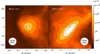 |
Fig. 1 B213-C2 and B213-C16 molecular hydrogen column density maps derived by Palmeirim et al. (2013), reconstructed at an angular resolution of 18.2″. Contour levels are (5,10,15 and 20) × 1021 cm−2 in the left panel and (5,10,15,20 and 25) × 1021 cm−2 in the right panel. The beam of the Yebes telescope in the Q band (HPBW≈42.5″) is plotted in each panel. |
4.1 Line profiles
We fit a Gaussian function to each observed line profile making use of the CLASS program. From these Gaussian profiles, we derived the peak velocity (vLSR), line width, line intensity (antenna temperature, T*A, corrected for atmospheric absorption and for antenna ohmic and spillover losses), and equivalent width. To convert the antenna temperature to the main-beam brightness temperature (TMB), the following expression was used:
 (1)
(1)
where ηeff is the forward efficiency and ηMB is the main-beam efficiency4. The results are shown in Tables A.1-A.2.
There are some species in B213-C2 whose transition lines present a double peak emission. These two velocity components, visible in a few rotational transitions, are displaced by approximately 1 km s−1, as is illustrated in both panels of Fig. 2. These two-peak profiles had been noticed in previous observations of this filament (e.g. Duvert et al. 1986; Goldsmith et al. 2008; Li & Goldsmith 2012; Hacar et al. 2013). The right panel of Fig. 2 shows the comparison between the observed line profiles for two different transitions of CH3OH. This comparison reveals that one of the velocity components present in the two-peaked transitions aligns in velocity with the component observed across all single-peaked transitions. This suggests that, unlike other dense cores such as L483 (Agúndez et al. 2019) or B335 (Esplugues et al. 2023), where the presence of multiple velocity peaks is due to self-absorption, the two-peak profiles observed in B213-C2 are most probably an indication of kinematically distinct components. We fit a Gaussian profile to each velocity peak in two-peaked transitions. However, because these two velocity components are only visible in a few low-energy transitions corresponding to abundant molecules, for subsequent calculations we exclusively considered the component visible across all observed transitions, at approximately 7 km s−1. The Gaussian fits obtained for both sources can be found in Zenodo.
4.2 Column densities: Rotational diagrams
For molecules with multiple detected transitions, we determined a rotational temperature (Trot) and column density (Ntot) using the rotational diagram method (Goldsmith & Langer 1999). For this, we assumed a single rotational temperature for all energy levels and local thermodynamic equilibrium (LTE). For optically thin emission, assuming that the source fills the beam, the column density, Nu, of the upper level is given by
 (2)
(2)
where gu is the statistical weight of the upper level, νul is the frequency of the transition,  is the integrated line intensity and Aul is the Einstein coefficient for spontaneous emission. Making use of this expression and applying Boltzmann’s equation, the following expression was derived:
 (3)
(3)
where Eu/k is the energy of the upper level and Q is the partition function at Trot, given by
 (4)
(4)
Considering Eq. (3) as a linear equation, the rotational temperature, Trot, and total column density, Ntot, can be derived from the slope and intercept of the regression line, respectively. The values of ln(Q) for each molecule at Trot were derived by linear interpolation from the data collected in CDMS5. The resulting rotational diagrams are shown in Figs. 3 and 4. The derived Trot and Ntot values are listed in Table A.3. The uncertainties shown in Table A.3 were obtained from the uncertainties in the least squares fit of the rotational diagrams.
The calculated rotational temperatures for both cores take values in the range of 4.68 ≲ Trot ≲ 9.17 K, with mean values and standard deviations of Trot, C2 = 8.43 ± 3.46 K and Trot, C16 = 6.38 ± 2.27 K. Two notable exceptions are OCS in C16 and HC7N in C2, with rotational temperatures of 2.62 K and 14.15 K, respectively. The low Trot derived for OCS hints at emission from a moderate- or low-density region, with the gas being subthermally excited. On the other hand, even though the derived value for HC7N is higher than expected for a cold dense core, considering the elevated uncertainty computed for this rotational temperature, this measure is still compatible with a rotational temperature of ~10 K. The rest of the calculated values are coherent with emission arising from a cold region. Previous ammonia mappings of Taurus cores derived a median temperature of 9.5 K (Jijina et al. 1999; Seo et al. 2015).
In those cases in which it was not possible to apply rotational diagrams, i.e., molecules with a single detected transition or molecules with multiple detected transitions but very similar upper level energies, we assigned each of these molecules a rotational temperature of 8 K, which is consistent with the Trot values previously derived by rotational diagrams. Column densities were then determined from Eqs. (2) and (3).
To estimate the impact of the uncertainties in the rotational temperature, we also calculated the total column densities and abundances assuming a fixed temperature of 8 K for those species with rotational diagrams (species in Figs. 3 and 4). The calculated values are shown in Table A.3. As can be derived from the table, the values obtained following both methods are compatible in the majority of cases.
The upper limits of the column densities were determined for the undetected species. The 3σ upper limit was derived from the rms (σ), the velocity resolution of the spectrum (∆v), and the line width (∆V), assuming ∆V = 1 km s−1. The upper limit to the equivalent width is given by
 (5)
(5)
Detected species in each source, number of observed lines, and minimum and maximum upper energies of the detected transitions.
4.3 Abundances
Fractional abundances relative to H2 were calculated from the column densities previously obtained, using the expression N(X)/N(H2) and the H2 column density and dust temperature maps of B213 (see Fig. 1), obtained by Palmeirim et al. (2013) derived from the Herschel Gould Belt Survey (André et al. 2010) and Planck data (Bernard et al. 2010) at an angular resolution of 18.2″. The total column density of H2, N(H2), is related to the visual extinction by the expression N(H2) = 1021 Av (Bohlin et al. 1978), with Av given by the extinction maps. Abundances were derived considering N(H2)C2 = 2.09 × 1022 cm−2 and N(H2)C16 = 2.48 × 1022 cm−2. The calculated abundances can be found in Table A.3.
For B213-C2, the derived fractional abundances take values of between 3.04 × 10⁻¹² and 3.35 × 10⁻⁹, with CC34S being the least abundant molecule and CS the most abundant. For C16, abundances take values of between 4.44 × 10⁻¹² and 2.59 × 10⁻⁹ with the least and most abundant molecules being, respectively, HSCN and CH3CCH.
 |
Fig. 2 Left : velocity components observed in CS overlapped with the two velocity components observed in C34S for the detected transitions in B213-C2. Right : superposition of the emission lines detected in B213-C2 for CH3OH with both one and two visible velocity components. |
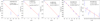 |
Fig. 3 Rotational diagrams for the detected molecules in B213-C2. The calculated values for the rotational temperature, Trot, and column density, Ntot, are indicated for each molecule. |
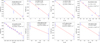 |
Fig. 4 Rotational diagrams for the detected molecules in B213-C16. The calculated values for the rotational temperature, Trot, and column density, Ntot, are indicated for each molecule. |
5 Discussion
5.1 Chemical comparison: C2 and C16
One of the goals of this paper is to explore the chemical evolution of starless cores in their process to become a collapsing core. Previous works suggest that the cores located in the northern part of B213, such as B213-C2, are more evolved than those located in the south (Spezzano et al. 2022; Esplugues et al. 2022). The wealth of species detected in our 7 mm survey allows us to perform a more complete chemical comparison. Figure 5 shows fractional abundance ratios between B213-C2 and B213-C16. As is seen in the figure, almost all the detected molecules are significantly more abundant in B213-C16. This would imply a higher molecular depletion in B213-C2, as is expected in a more evolved core. The only exceptions to this rule are l-C3H and HOCO+.
The decrease in the density of stars from north to south makes B213-C2, located in the northern part of the filament, more likely to be affected by the presence of low-mass stars located nearby. The cones of the outflows of these stars carve out the medium, allowing the interstellar radiation field to penetrate the molecular cloud (Spezzano et al. 2022). Although the inner parts of the cloud are shielded from UV radiation by the dust, the subsequent exposure to UV radiation in the outer regions could contribute to reduce abundances for some species and an increase in the abundances of certain molecules such as HOCO+, related with irradiated ices (Minh et al. 1991). In the same line, the radical l-C3H is known to present enhanced abundances in photodissociation regions (Pety et al. 2012; Guzmán et al. 2015). As can be seen in Fig. 5, these molecules display similar fractional abundances in both sources.
Another possible cause of the chemical differentiation observed between C16 and C2 could be the accretion of background molecular gas. Goldsmith et al. (2008) and Palmeirim et al. (2013) found that the B213 region of the B213/L1495 filament is surrounded by a large number of low-density striations that are oriented approximately perpendicular to the main filament and parallel to the magnetic field. Blueshifted and red-shifted components in both 12CO(1-0) and 13CO(1-0) emission are also visible to the southwest and northeast of the B213 filament. This morphology is suggestive of mass accretion along the field lines into the filament. Shimajiri et al. (2019) proposed that the filament was initially formed by large-scale compression of HI gas and is now growing in mass as a result of the gravitational accretion of molecular gas of the ambient cloud. It is possible that this accretion of ambient material into this part of the B213/L1495 filament along the magnetic field lines is enhancing the molecular abundances in the embedded cores. However, these low-density striations are not present in the B7-B10 region (see Fig. 2 of Hacar et al. 2013) of the B213/L1495 filament, where C2 is located. Chapman et al. (2011) indicated that above core 7, where the filament presents a sharp turn to the north, the magnetic field switches from being perpendicular to the filament to becoming parallel. In the presence of a magnetic field, motions of ionized gas encounter a significant magnetic resistance perpendicular to the field lines (Nagai et al. 1998) and, under these conditions, the accretion of background material is mainly parallel to the field lines.
Finally, as was commented on above, the lower abundances observed in C2 could stem from the evolutionary state of the cores, with B213-C2 constituting a more evolved object, closer to the pre-stellar core phase. A higher density would cause the depletion of some molecules, which would condense out onto dust grain surfaces. This would be reflected in reduced abundances in B213-C2. These factors are not exclusive, and the observed differences in molecular abundances between the two sources are most likely the result of their addition.
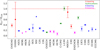 |
Fig. 5 Fractional abundance ratios between B213-C2 and B213-C16, for all the detected species. Lower limits of the ratios, corresponding to molecules detected in B213-C16 but not in B213-C2, are marked with downward triangles. Conversely, upper limits of the ratios, for molecules detected in B213-C2 but not in B213-C16, are indicated with upward triangles. |
5.2 Chemical comparison with other sources
Once a protostar is formed, it heats the surrounding material, increasing dust temperature, and releasing the icy molecules to the gas phase. At this early stage, the cold envelope is still infalling and its chemical composition remains similar to the parent core. Figures 6 and 7 show fractional abundances relative to H2 in C2 and C16 compared with those in five reference sources representative of the earliest stages of the formation of a low-mass star: TMC-1, B 335, B1-b, L1527, and L483.
The considered sources present different evolutionary stages, including both starless cores and cores with indications of star formation. Taurus Molecular Cloud-1 (TMC-1) is a cold dense cloud with no signs of star formation, located at the centre of the Taurus Molecular Cloud at a distance of  pc (Galli et al. 2019). Barnard 335 (B 335) is a prototypical example of a large, isolated dust globule (Keene et al. 1980), which is associated with an embedded far-infrared source, IRAS 19347+0727 (Keene et al. 1983). The presence of saturated complex organic molecules (COMs) identifies B 335 as a hot corino (Cazaux et al. 2003; Imai et al. 2016). The source Barnard 1b (B1-b) is a dark cloud that hosts two young protostellar objects, B1b-N and B1b-S (Huang & Hirano 2013). The high HCS+∕CS ratio for B 335 (Esplugues et al. 2023) compared to the value observed in B1-b (Fuente et al. 2016) suggests an early evolutionary stage of B 335 compared to B1-b, as rate coefficients for ion-CS reactions increase at low temperatures (Clary et al. 1985). On the other hand, the source L483 is an optical dark cloud with an embedded infrared source, which is classified as a Class 0/I object (Tafalla et al. 2000; Agúndez et al. 2019). Finally, the dense core L1527 contains a solar-type Class 0/I protostar, IRAS04368+2557 (Yoshida et al. 2019). Therefore, the sources can be approximately ordered in an evolutionary sequence as with starless cores B213-C2 and B213-C16 being in an evolutionary state between TMC-1 and B 335. The order of the plots in Figs. 6 and 7 follows this evolutionary sequence.
For TMC-1, column densities are mostly taken from the line survey of the cyanopolyyne peak position of TMC-1 (TMC-1(CP)) carried out with the Nobeyama 45 m telescope (Kaifu et al. 2004), revised by Gratier et al. (2016), and also from the QUIJOTE line survey of TMC-1 (CP) (Cernicharo et al. 2024) and from Agúndez & Wakelam (2013). In the case of the source B 335, abundances are based on a study of its sulfur chemistry through observations in the spectral range λ = 7, 3 and 2 mm, conducted with the Yebes-40 m and IRAM-30 m telescopes (Esplugues et al. 2023). B1-b data is based on the chemical studied carried out by Fuente et al. (2016). Abundances for L1527 were taken from a λ = 3 mm line survey conducted with the Nobeyama-45 m telescope (Yoshida et al. 2019). Finally, for the source L483, colum densities were taken from the λ = 3 mm line survey carried out with the IRAM-30 m telescope in the 80-116 GHz frequency range (Agúndez et al. 2019). Most of the abundances plotted in Figs. 6 and 7 have been measured at similar spatial scales (3000-6000 au), which makes their comparison reasonable. However, B 335 and L1527 present smaller spatial scales.
As can be seen in Figs. 6 and 7, TMC-1 presents the highest abundances of all the compared sources. This is to be expected, as previous studies have shown that TMC-1 is a particularly molecule-rich dark cloud, especially in carbon chains (Agúndez & Wakelam 2013). A high cosmic-ray ionization rate, ζH2, has been suggested as an explanation for the richness of TMC-1 in this type of molecule (Agúndez & Wakelam 2013). This target is considered to be a prototype for the starless core stage prior to the collapse.
The source B 335 presents a clear chemical differentiation with respect to C2 and C16. The overabundance of sulfur-bearing species is particularly pronounced when comparing abundances of sulfur carbon chains. Recent studies on sulfur chemistry in B 335 have identified it as an especially rich source in this type of molecule, unlike other Class 0 sources (Esplugues et al. 2023). B 335 presents an early evolutionary stage comparable to the ages of pre-stellar condensations (Caselli & Ceccarelli 2012). This could be the result of the isolated source nature of B 335 compared to other protostars formed in dense molecular clouds. Accretion of diffuse cloud material has also been proposed as a possible cause of the different chemistry observed in B 335 (Esplugues et al. 2023). In any case, the lower molecular abundances observed in both C2 and C16 with respect to B 335 are likely a result of the chemical richness of this peculiar source.
The upper right panels of Figs. 6 and 7 show that the abundances of hydrocarbons and oxygen-bearing molecules in B1-b are of the same order as in C2 and C16. However, marked chemical differentiation is observed for S-bearing molecules. This difference could be explained in terms of freeze-out, as the sources present varying degrees of sulfur depletion. Previous works based on methanol observations suggest a chemical differentiation between the northern and southern cores of the B213 filament (Spezzano et al. 2022; Punanova et al. 2022). A recent study of the H2CS deuterated compounds (Esplugues et al. 2022) showed that the cores located in the northern part of the filament are more chemically evolved than the southern cores. Moreover, based on observations of NS, Hily-Blant et al. (2022) proposed a correlation between sulfur depletion and chemical age, with more evolved cores presenting a higher sulfur depletion. On the other hand, the source B1-b presents a moderate sulfur depletion ([S/H] ~ 6.0 × 10⁻⁷), which could be the consequence of the star formation activity in the region with multiple outflows in the surroundings or the result of the rapid collapse of B1-b (Fuente et al. 2016). These differences in sulfur depletion could explain the higher abundances of S-bearing molecules observed in B1-b with respect to C2, located in the northern part of the B213 filament, and the lower abundances in B1-b with respect to C16, located south of the filament. The bottom panels of Figs. 6 and 7 show that, in general, L1527 presents lower molecular abundances than C2 and C16, with the exception of hydrocarbons, which take higher or similar values to those observed in C2. Abundances in L483 are overabundant with respect to C2 and underabundant when comparing with C16. Among carbon-chain molecules, the CnHm species seem especially abundant in both L1527 and L483, presenting similar values to those observed in C16, and even higher in the case of L483. A longer lifetime than the other carbon-chain molecules has been proposed as a possible cause of the high abundances of these molecules. Otherwise, the CnHm molecules may be regenerated near the protostar, as both L1527 and L483 are warm carbon-chain chemistry (WCCC) sources (Sakai et al. 2008; Oya et al. 2017). In the scenario of the production of unsaturated carbon chains, often referred to as WCCC (Sakai & Yamamoto 2013), this regeneration process would be driven by the evaporation of CH4 due to protostellar activity, as CH4 has a relatively low sublimation temperature (~30 K). The higher temperatures in the vicinity of the protostar can cause the CnHm to evaporate from dust grains, with the subsequent carbon-chain production in the gas phase. However, under the physical conditions prevailing in systems that result in WCCC, the formation of HCnN is slower than that of CnHm, due to slow neutral-neutral reactions, which would suppress the abundances of HCnN and other N-bearing species (Turner et al. 1998; Sakai et al. 2008; Yoshida et al. 2019). As can be seen in the bottom panels of Fig. 6, the abundance of HC5N in both L1527 and L483, takes similar values to the ones observed in C2.
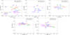 |
Fig. 6 Fractional abundance ratios between B213-C2 and five reference sources: TMC-1, B335, B1-b, L1527, and L483. Upper and lower limits are indicated with downward and upward triangles, respectively. L483: Agúndez et al. (2019). TMC-1: Gratier et al. (2016); Cernicharo et al. (2024); Agúndez & Wakelam (2013). L1527: Yoshida et al. (2019). B335: Esplugues et al. (2023). B1-b: Fuente et al. (2016); Loison et al. (2017); Widicus Weaver et al. (2017). N(H2) values used to obtain fractional abundances are 7.60 × 1022 cm−2 for B1-b (Daniel et al. 2013), and 1.80 × 1022 cm−2 for TMC-1 (Palmeirim et al. 2013; Rodríguez-Baras et al. 2021). Physical scales for each source are indicated in the upper left corner. |
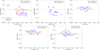 |
Fig. 7 Fractional abundance ratios between B213-C16 and five reference sources: TMC-1, B335, B1-b, L1527 and L483. Upper and lower limits are indicated with downward and upward triangles, respectively. L483: Agúndez et al. (2019). TMC-1: Gratier et al. (2016); Cernicharo et al. (2024); Agúndez & Wakelam (2013). L1527: Yoshida et al. (2019). B335: Esplugues et al. (2023). B1-b: Fuente et al. (2016); Loison et al. (2017); Widicus Weaver et al. (2017). N(H2) values used to obtain fractional abundances are 7.60 × 1022 cm−2 for B1-b (Daniel et al. 2013), and 1.80 × 1022 cm−2 for TMC-1 (Palmeirim et al. 2013; Rodríguez-Baras et al. 2021). Physical scales for each source are indicated in the upper left corner. |
6 Comparison with chemical models
To better constrain the physical and chemical properties of both C2 and C16, we compared the observational data to a set of chemical models. These models were computed by a neural emulator of the astrochemical code NAUTILUS 1.1 based on conditional neural fields (Asensio Ramos et al. 2024). This emulator reproduces Nautilus predictions with a precision well below 0.1 dex, allowing us to carry out a broad exploration of the space parameter in a reasonable time.
NAUTILUS 1.1 (Ruaud et al. 2016) is a three-phase model that considers gas, grain surface, and grain mantle phases, along with their interactions. Given a set of physical and chemical input parameters, it solves the kinetic equations for the gas-phase and the solid species at the surface of interstellar dust grains, calculating the evolution with time of chemical abundances. The use of neural networks to simulate the behaviour of chemical models considerably reduces the computation time, allowing a more in-depth exploration of the parameter space and reducing the uncertainties for all the considered species.
6.1 Parameter space
We ran a set of models with typical physical conditions in dark clouds, which were selected randomly in the intervals defined in Table 3. All the parameters except for the temperature, which is linearly sampled, are sampled uniformly in log space as they mostly span several orders of magnitude. The visual extinction takes the fixed values 10.5 and 12.4 for C2 and C16, respectively (Palmeirim et al. 2013; Rodríguez-Baras et al. 2021).
We considered chemical ages, t, between early chemistry (0.01 Myr) and steady-state chemistry (10 Myr). The sulfur elemental abundance [S/H] varied between the cases of no depletion, [S/H] = 1.5 × 10⁻⁵, and high-depletion, [S/H] = 7.5 × 10⁻⁸. These values correspond to different estimates of sulfur depletion in star-forming regions (Esplugues et al. 2014; Vastel et al. 2018; Navarro-Almaida et al. 2020, 2021). The cosmic-ray ionization rate, ζH2, was allowed to take values between ζH2 = 10−17 s−1, found in dense and evolved cores (Caselli et al. 2002), and ζH2 = 5 × 10⁻¹⁶ s−1, expected in diffuse molecular gas (Neufeld & Wolfire 2017). We considered χUV = 50 as the upper limit for the UV field strength in units of Draine field (Draine 1978), based on the values derived toward photon-dominated regions such as the Horsehead nebula (Pety et al. 2005; Goicoechea et al. 2006; Rivière-Marichalar et al. 2019).
6.2 Methodology
Our aim is to determine the values of t, nH, ζH2, [S/H], χUV, and T that best fit the observational data for each core. We need to select a parameter in order to describe the goodness of each model. The standard chi-squared χ2 is not adequate to estimate errors when the molecular abundances included in the fit differ from the observed abundances by several orders of magnitude. For this reason, we used the parameter Ddiff, defined as
![Mathematical equation: D_{diff} \ (t)=\frac{1}{n_{obs}}\sum_{i}[log_{10}(X^{i}_{mod})(t)-log_{10}(X^{i}_{obs})]^{2}](/articles/aa/full_html/2026/02/aa56867-25/aa56867-25-eq8.png) (6)
(6)
where nobs is the number of detected species in the source,  is the model predicted abundance for the i species at a time, t, and
  is the abundance derived from the observations. This parameter is the square of the “disagreement parameter” that has been previously used in astrochemistry by different authors (see e.g., Wakelam et al. 2006; Vastel et al. 2018; Fuente et al. 2023; Taillard et al. 2025).
First, we ran the models allowing the parameter t to vary among a range of discrete values in the interval 104−107 Myr, with the purpose of determining the evolution time that best reproduces the observational data. We then ran a new set of models fixing t to the best-fitting value previously determined. Reasonable intervals for the rest of the parameters were obtained from a set of best-fitting models including those whose Ddiff parameter differs from the minimum Ddiff value by less than 1%.
In our fitting, we used the molecular abundances derived in this paper as well as those of C18O, H13CO+, H13CN, SO, HNC, and H2S derived by Rodríguez-Baras et al. (2021) using the database of the IRAM LP GEMS database6. The abundances for CS, C18O, H13CO+, and H13CN were derived from those of C34S, CO, HCO+, and HCN, considering the isotopic ratios 32S∕34S = 22.5, 12C∕13C = 60, and 16O∕18O = 550 (Wilson & Rood 1994; Savage et al. 2002; Gratier et al. 2016).
Chemical model parameters.
6.3 Comparison with observations
Our first aim is to determine the chemical age, t, that best reproduces the observational data for each source. Figure 8 shows the Ddiff parameter as a function of time for a set of 103 models generated with the physical conditions listed in Table 3. From both panels of Fig. 8, we have deduced that the observed abundances are best fit assuming early time chemistry (t ~ 0.1 Myr), which is consistent with the idea that this filament is still accreting background material of the ambient cloud, keeping the gas chemistry far from the steady state (Fuente et al. 2023).
To constrain the values for the rest of the parameters, we ran another set of models, fixing the chemical age, t, to the best-fitting value for each core. Figure 9 shows the comparison between the observed abundances and the predictions of the bestfitting models shown in Table 4. Horizontal dashed lines indicate discrepancies by factors of 2, 5, and 10. Most molecules are well reproduced within a factor of <5, including CH3OH, and other COMs, such as cyanopolynes. However, a few are poorly reproduced by the model with discrepancies of more than one order of magnitude. In particular, the abundances for HNC, H2S, and the carbon chains C2S, and C3O are poorly reproduced in the two studied cores. The molecules HNC and H2S are over-reproduced by a factor of 10. In the case of HNC, the abundance derived from the GEMS database is uncertain since the observed line, HNC J=1→0, is expected to be optically thick in dense cores. Tasa-Chaveli et al. (2025) presented new observations of HN13C in C2 and C16. Assuming HN12C∕ HN13C=60, we estimate HNC abundances a factor of ~10 higher than those used in the fitting, in better agreement with model predictions. Opacity effects could also be significant in the case of H2S. Taking the N(H324S) column density derived by Rodríguez-Baras et al. (2023) toward C2, and assuming 32S∕34S= 22.5, we obtain a H2S abundance of H2S ~2.7 times higher than the value previously obtained by Rodríguez-Baras et al. (2021). Rodríguez-Baras et al. (2023) did not detect H342S toward C16. Even taking into account an uncertainty of a factor of ~3 in the H2S abundance, model predictions remain higher than the observed values. The cases of C2S and C3O cannot be attributed to opacity effects, according to the observed CCS∕CC34S and CCCS∕CCC34S column density ratios measured in this work. The poor agreement of the model predictions with observations is more likely related to uncertainties in the chemistry of these species. Our data suggests that although our state-of-the-art chemical models are doing a good job at predicting some COMs and nitrogen-bearing species, the description of sulfur chemistry and especially the formation of the sulfur and oxygen carbon chains needs to be improved.
To test the robustness of our modeling, we repeated the fitting assuming different chemical times. As is shown in Fig. 8, the best-fitting models for C2 reach Ddiff values within a 1% difference with respect to Ddiff, min for t ~ 0.1 Myr and remain within a 5 % difference for t values in the interval 0.10-0.17 Myr. For C16, we find larger variation, with the best-fitting models reaching Ddiff values within a 1% difference for t ~ 0.17 Myr, and up to a 5% difference for t values in the interval 0.13-1 Myr. To evaluate the uncertainties that fixing the time can introduce in the fitting of C16, we repeated it for t = 1 Myr. We found that the main difference between the different times is a decrease in density for longer times. Specifically, we obtain a density about 3 times lower, nH ~ 4.0 × 104 cm−3, adopting t = 1 Myr. The variations in the rest of parameters are within the uncertainties. Tasa-Chaveli et al. (2025) estimated densities of nH ~ 2.0 ×105 cm−3 toward this core based on a multi-transition analysis of DNC. This result provides further support for our best-fitting model in Table 4 being the more accurate one with the information available until now.
Chemical differences between starless cores can be due to different evolutionary stages, environmental conditions, and also the cloud history. Our fitting results show that C2 is best reproduced by nH = (1.94-1.99) × 105 cm−3, while C16 is best-fit by nH = (1.29-1.69) × 105 cm−3. These higher molecular hydrogen densities in C2 with respect to C16 are consistent with C2 being a denser, more evolved object, closer to the pre-stellar core phase. Regarding the sulfur elemental abundance, it also hints at this possibility, as C2 presents a higher sulfur depletion, which is suggestive of a more advanced evolutionary stage in agreement with Hily-Blant et al. (2022). Despite being embedded in a harsher environment, with a higher number of low-mass stars located nearby, C2 seems better fit by low cosmic-ray ionization rates (ζH2 = (1.33-1.63) × 10−17 s−1). This could also be related to a higher density in C2, as ζH2 is attenuated by an increasing gas column density (Padovani et al. 2009).
All physical and chemical indicators point to a more evolved stage for C2 than for C16, consistent with Esplugues et al. (2022).
Based on our chemical model, we cannot constrain the environmental UV field since the impinging radiation is strongly attenuated at high optical depths. The chemical age derived from our observations is similar in the two starless cores, contrary to the results based on other evolutionary indicators. Our 0D chemical model does not account for physical and chemical gradients along the line of sight. It does not account for either the dynamical evolution or turbulence effects, which could affect molecular abundances, especially of sulfurated species (Beitia-Antero et al. 2024). More sophisticated models accounting for chemistry and dynamics in a consistent way should be used to gain further insights into the accreting and collapsing history of this complex star-forming filament and the cores within it.
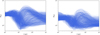 |
Fig. 8 Ddiff (t) for a set of 103 models considering the physical conditions listed for B213-C2 (left) and B213-C16 (right). |
 |
Fig. 9 Ratios between the best-fitting model prediction and the observed abundances for B213-C2 (left) and B213-C16 (right), indicated with blue bars. Discrepancies between model and observations of a factor 10, 5 and 2 are indicated with dashed blue, red, and orange lines, respectively. |
Parameters corresponding to the best-fitting models.
7 Summary and conclusions
We have carried out a λ = 7 mm line survey in the 31.350.6 GHz frequency range for the starless cores B213-C2 and B213-C16, using the Yebes 40-m telescope. We detected 122 emission lines, 56 of them corresponding to B213-C2 and the remaining 66 to B213-C16. Including isotopologs, 22 species were detected in B213-C2, while 25 were detected in B213-C16. The observed molecules include O-bearing molecules (CH3CHO, CH3OH, HOCO+), hydrocarbons (CH3CCH, c-C3H2, l-C3H, l-C3H2), N-bearing molecules (CH3CN, HC5N, HC7N, CH2CHCN), and S-bearing molecules (CS, H2CS, HCNS, HSCN, HCS+, OCS, SO2, CCS, C3S, 13CS, C34S, C33S, CC34S, CCC34S).
To determine column densities, we used the rotational diagram method, deriving rotational temperatures mostly in the range of 5 ≲ Trot ≲ 9 K, consistent with emission arising from a cold source. In general, fractional molecular abundances in B213-C2 are lower than in B213-C16. This could be the result of environmental factors such as C2 presenting a higher exposure to UV radiation from nearby low-mass stars, or a rejuvenation of the chemistry in C16 due to the accretion of background molecular gas. The lower molecular abundances in C2 could also stem from the evolutionary state of the cores, with C2 constituting a denser, more evolved object closer to the pre-stellar phase. A higher density would cause the depletion of some molecules, which would condense out onto dust grain surfaces.
The molecular abundances in both cores were also compared with those of five reference sources (TMC-1, B 335, B1-b, L1527, and L483) with different evolutionary stages. TMC-1 presents the highest abundances of all the compared sources. This is to be expected, as TMC-1 has been shown to be a particularly molecule-rich dark cloud. The source B 335 presents a clear chemical differentiation with respect to C2 and C16, with considerably higher abundances of sulfur carbon chains. This is probably due to B 335 being especially rich in this type of molecule, unlike other Class 0 sources. Hydrocarbons and oxygen-bearing molecules in B1-b are of the same order as in C2 and C16. However, marked chemical differentiation is observed for S-bearing molecules. This difference could be explained by the varying degrees of sulfur depletion in this source, with B1-b presenting moderate sulfur depletion (DS = 25). In general, L1527 presents lower molecular abundances than C2 and C16, while abundances in L483 are overabundant with respect to C2 and underabundant compared to C16.
The comparison with chemical models shows that both cores are best fit with t ~ 0.1 Myr. However, the parameters corresponding to the best-fitting models hint at C2 being at a more advanced evolutionary stage, as it presents a higher molecular hydrogen density and sulfur depletion than C16, and a lower cosmic-ray ionization rate. More complex simulations, coupling dynamics and chemistry, are required to describe in detail the evolution of a dense core during its collapse.
Data availability
The Gaussian fits obtained for both sources can be found at Zenodo.
Acknowledgements
This project has received funding from the European Research Council (ERC) under the European Union's Horizon Europe research and innovation programme ERC-AdG-2022 (GA No. 101096293). Views and opinions expressed are however those of the author(s) only and do not necessarily reflect those of the European Union or the European Research Council Executive Agency. Neither the European Union nor the granting authority can be held responsible for them. AF, MRB, GE, PRM and BT also thank project PID2022-137980NB-I00 funded by the Spanish Ministry of Science and Innovation/State Agency of Research MCIN/AEI/10.13039/501100011033 and by “ERDF A way of making Europe.” BT also thanks project PID2023-147545NB-I00. AAR acknowledges funding from the Agencia Estatal de Investigación del Ministerio de Ciencia, Innovación y Universidades (MCIU/AEI) under grant “Polarimetric Inference of Magnetic Fields” and the European Regional Development Fund (ERDF) with reference PID2022-136563NB-I00/10.13039/501100011033. The authors thank the anonymous referee for their valuable suggestions.
References
- Agúndez, M., & Wakelam, V. 2013, Chem. Rev., 113, 8710 [Google Scholar]
- Agúndez, M., Marcelino, N., Cernicharo, J., Roueff, E., & Tafalla, M. 2019, A&A, 625, A147 [Google Scholar]
- André, P., Men’shchikov, A., Bontemps, S., et al. 2010, A&A, 518, L102 [NASA ADS] [CrossRef] [EDP Sciences] [Google Scholar]
- Araki, M., Takano, S., Sakai, N., et al. 2017, ApJ, 847, 51 [Google Scholar]
- Asensio Ramos, A., Westendorp Plaza, C., Navarro-Almaida, D., et al. 2024, MNRAS, 531, 4930 [NASA ADS] [CrossRef] [Google Scholar]
- Bacmann, A., Taquet, V., Faure, A., Kahane, C., & Ceccarelli, C. 2012, A&A, 541, L12 [NASA ADS] [CrossRef] [EDP Sciences] [Google Scholar]
- Beitia-Antero, L., Fuente, A., Navarro-Almaida, D., et al. 2024, A&A, 688, A188 [NASA ADS] [CrossRef] [EDP Sciences] [Google Scholar]
- Benson, P. J., & Myers, P. C. 1989, ApJS, 71, 89 [Google Scholar]
- Bergin, E. A., & Tafalla, M. 2007, ARA&A, 45, 339 [Google Scholar]
- Bernard, J. P., Paradis, D., Marshall, D. J., et al. 2010, A&A, 518, L88 [NASA ADS] [CrossRef] [EDP Sciences] [Google Scholar]
- Bohlin, R. C., Savage, B. D., & Drake, J. F. 1978, ApJ, 224, 132 [Google Scholar]
- Bracco, A., Palmeirim, P., André, P., et al. 2017, A&A, 604, A52 [NASA ADS] [CrossRef] [EDP Sciences] [Google Scholar]
- Cambrésy, L. 1999, A&A, 345, 965 [NASA ADS] [Google Scholar]
- Caselli, P., & Ceccarelli, C. 2012, A&A Rev., 20, 56 [NASA ADS] [Google Scholar]
- Caselli, P., Walmsley, C. M., Terzieva, R., & Herbst, E. 1998, ApJ, 499, 234 [Google Scholar]
- Caselli, P., Walmsley, C. M., Zucconi, A., et al. 2002, ApJ, 565, 344 [Google Scholar]
- Cazaux, S., Tielens, A. G. G. M., Ceccarelli, C., et al. 2003, ApJ, 593, L51 [CrossRef] [Google Scholar]
- Cernicharo, J., & Guelin, M. 1987, A&A, 176, 299 [NASA ADS] [Google Scholar]
- Cernicharo, J., Agúndez, M., Cabezas, C., et al. 2024, A&A, 682, L4 [NASA ADS] [CrossRef] [EDP Sciences] [Google Scholar]
- Chapman, N. L., Goldsmith, P. F., Pineda, J. L., et al. 2011, ApJ, 741, 21 [NASA ADS] [CrossRef] [Google Scholar]
- Clary, D. C., Smith, D., & Adams, N. G. 1985, Chem. Phys. Lett., 119, 320 [CrossRef] [Google Scholar]
- Daniel, F., Gérin, M., Roueff, E., et al. 2013, A&A, 560, A3 [NASA ADS] [CrossRef] [EDP Sciences] [Google Scholar]
- Draine, B. T. 1978, ApJS, 36, 595 [Google Scholar]
- Duvert, G., Cernicharo, J., & Baudry, A. 1986, A&A, 164, 349 [NASA ADS] [Google Scholar]
- Esplugues, G. B., Viti, S., Goicoechea, J. R., & Cernicharo, J. 2014, A&A, 567, A95 [NASA ADS] [CrossRef] [EDP Sciences] [Google Scholar]
- Esplugues, G., Fuente, A., Navarro-Almaida, D., et al. 2022, A&A, 662, A52 [NASA ADS] [CrossRef] [EDP Sciences] [Google Scholar]
- Esplugues, G., Rodríguez-Baras, M., San Andrés, D., et al. 2023, A&A, 678, A199 [NASA ADS] [CrossRef] [EDP Sciences] [Google Scholar]
- Fuente, A., Cernicharo, J., Roueff, E., et al. 2016, A&A, 593, A94 [NASA ADS] [CrossRef] [EDP Sciences] [Google Scholar]
- Fuente, A., Navarro, D. G., Caselli, P., et al. 2019, A&A, 624, A105 [NASA ADS] [CrossRef] [EDP Sciences] [Google Scholar]
- Fuente, A., Rivière-Marichalar, P., Beitia-Antero, L., et al. 2023, A&A, 670, A114 [NASA ADS] [CrossRef] [EDP Sciences] [Google Scholar]
- Galli, P A. B., Loinard, L., Bouy, H., et al. 2019, A&A, 630, A137 [NASA ADS] [CrossRef] [EDP Sciences] [Google Scholar]
- Goicoechea, J. R., Pety, J., Gerin, M., et al. 2006, A&A, 456, 565 [NASA ADS] [CrossRef] [EDP Sciences] [Google Scholar]
- Goldsmith, P. F., & Langer, W. D. 1978, ApJ, 222, 881 [Google Scholar]
- Goldsmith, P. F., & Langer, W. D. 1999, ApJ, 517, 209 [Google Scholar]
- Goldsmith, P. F., Heyer, M., Narayanan, G., et al. 2008, ApJ, 680, 428 [Google Scholar]
- Gratier, P., Majumdar, L., Ohishi, M., et al. 2016, ApJS, 225, 25 [Google Scholar]
- Guzmán, V. V., Pety, J., Goicoechea, J. R., et al. 2015, ApJ, 800, L33 [CrossRef] [Google Scholar]
- Hacar, A., Tafalla, M., Kauffmann, J., & Kovács, A. 2013, A&A, 554, A55 [NASA ADS] [CrossRef] [EDP Sciences] [Google Scholar]
- Hily-Blant, P., Pineau des Forêts, G., Faure, A., & Lique, F. 2022, A&A, 658, A168 [NASA ADS] [CrossRef] [EDP Sciences] [Google Scholar]
- Hirota, T., Sakai, N., & Yamamoto, S. 2010, ApJ, 720, 1370 [Google Scholar]
- Huang, Y.-H., & Hirano, N. 2013, ApJ, 766, 131 [Google Scholar]
- Imai, M., Sakai, N., Oya, Y., et al. 2016, ApJ, 830, L37 [CrossRef] [Google Scholar]
- Jijina, J., Myers, P. C., & Adams, F. C. 1999, ApJS, 125, 161 [Google Scholar]
- Juvela, M., Ristorcelli, I., Pagani, L., et al. 2012, A&A, 541, A12 [NASA ADS] [CrossRef] [EDP Sciences] [Google Scholar]
- Kaifu, N., Ohishi, M., Kawaguchi, K., et al. 2004, PASJ, 56, 69 [Google Scholar]
- Keene, J., Hildebrand, R. H., Whitcomb, S. E., & Harper, D. A. 1980, ApJ, 240, L43 [NASA ADS] [CrossRef] [Google Scholar]
- Keene, J., Davidson, J. A., Harper, D. A., et al. 1983, ApJ, 274, L43 [NASA ADS] [CrossRef] [Google Scholar]
- Lattanzi, V., Bizzocchi, L., Vasyunin, A. I., et al. 2020, A&A, 633, A118 [NASA ADS] [CrossRef] [EDP Sciences] [Google Scholar]
- Li, D., & Goldsmith, P. F. 2012, ApJ, 756, 12 [NASA ADS] [CrossRef] [Google Scholar]
- Loison, J.-C., Agúndez, M., Wakelam, V., et al. 2017, MNRAS, 470, 4075 [Google Scholar]
- Luhman, K. L., Mamajek, E. E., Allen, P. R., & Cruz, K. L. 2009, ApJ, 703, 399 [NASA ADS] [CrossRef] [Google Scholar]
- Marsh, K. A., Griffin, M. J., Palmeirim, P., et al. 2014, MNRAS, 439, 3683 [NASA ADS] [CrossRef] [Google Scholar]
- Minh, Y. C., Brewer, M. K., Irvine, W. M., Friberg, P., & Johansson, L. E. B. 1991, A&A, 244, 470 [NASA ADS] [Google Scholar]
- Mizuno, A., Onishi, T., Yonekura, Y., et al. 1995, ApJ, 445, L161 [NASA ADS] [CrossRef] [Google Scholar]
- Molinari, S., Swinyard, B., Bally, J., et al. 2010, A&A, 518, L100 [NASA ADS] [CrossRef] [EDP Sciences] [Google Scholar]
- Müller, H. S. P., Schlöder, F., Stutzki, J., & Winnewisser, G. 2005, J. Mol. Struct., 742, 215 [Google Scholar]
- Mumma, M. J., & Charnley, S. B. 2011, ARA&A, 49, 471 [Google Scholar]
- Nagai, T., Inutsuka, S.-i., & Miyama, S. M. 1998, ApJ, 506, 306 [NASA ADS] [CrossRef] [Google Scholar]
- Narayanan, G., Heyer, M. H., Brunt, C., et al. 2008, ApJS, 177, 341 [NASA ADS] [CrossRef] [Google Scholar]
- Navarro-Almaida, D., Le Gal, R., Fuente, A., et al. 2020, A&A, 637, A39 [NASA ADS] [CrossRef] [EDP Sciences] [Google Scholar]
- Navarro-Almaida, D., Fuente, A., Majumdar, L., et al. 2021, A&A, 653, A15 [NASA ADS] [CrossRef] [EDP Sciences] [Google Scholar]
- Navarro-Almaida, D., Lebreuilly, U., Hennebelle, P., et al. 2024, A&A, 685, A112 [NASA ADS] [CrossRef] [EDP Sciences] [Google Scholar]
- Neufeld, D. A., & Wolfire, M. G. 2017, ApJ, 845, 163 [Google Scholar]
- Öberg, K. I., Boogert, A. C. A., Pontoppidan, K. M., et al. 2011, ApJ, 740, 109 [Google Scholar]
- Öberg, K. I., Facchini, S., & Anderson, D. E. 2023, ARA&A, 61, 287 [Google Scholar]
- Onishi, T., Mizuno, A., Kawamura, A., Ogawa, H., & Fukui, Y. 1996, ApJ, 465, 815 [NASA ADS] [CrossRef] [Google Scholar]
- Onishi, T., Mizuno, A., Kawamura, A., Tachihara, K., & Fukui, Y. 2002, ApJ, 575, 950 [NASA ADS] [CrossRef] [Google Scholar]
- Oya, Y., Sakai, N., Watanabe, Y., et al. 2017, ApJ, 837, 174 [Google Scholar]
- Padoan, P., Cambrésy, L., & Langer, W. 2002, ApJ, 580, L57 [NASA ADS] [CrossRef] [Google Scholar]
- Padovani, M., Galli, D., & Glassgold, A. E. 2009, A&A, 501, 619 [NASA ADS] [CrossRef] [EDP Sciences] [Google Scholar]
- Padovani, M., Hennebelle, P., & Galli, D. 2013, A&A, 560, A114 [NASA ADS] [CrossRef] [EDP Sciences] [Google Scholar]
- Palmeirim, P., André, P., Kirk, J., et al. 2013, A&A, 550, A38 [NASA ADS] [CrossRef] [EDP Sciences] [Google Scholar]
- Pety, J., Teyssier, D., Fossé, D., et al. 2005, A&A, 435, 885 [NASA ADS] [CrossRef] [EDP Sciences] [Google Scholar]
- Pety, J., Gratier, P., Guzmán, V., et al. 2012, A&A, 548, A68 [NASA ADS] [CrossRef] [EDP Sciences] [Google Scholar]
- Pickett, H. M., Poynter, R. L., Cohen, E. A., et al. 1998, J. Quant. Spec. Radiat. Transf., 60, 883 [Google Scholar]
- Punanova, A., Caselli, P., Pineda, J. E., et al. 2018, A&A, 617, A27 [NASA ADS] [CrossRef] [EDP Sciences] [Google Scholar]
- Punanova, A., Vasyunin, A., Caselli, P., et al. 2022, ApJ, 927, 213 [CrossRef] [Google Scholar]
- Rebull, L. M., Padgett, D. L., McCabe, C. E., et al. 2010, ApJS, 186, 259 [NASA ADS] [CrossRef] [Google Scholar]
- Rivière-Marichalar, P., Fuente, A., Goicoechea, J. R., et al. 2019, A&A, 628, A16 [Google Scholar]
- Rodríguez-Baras, M., Fuente, A., Riviére-Marichalar, P., et al. 2021, A&A, 648, A120 [NASA ADS] [CrossRef] [EDP Sciences] [Google Scholar]
- Rodríguez-Baras, M., Esplugues, G., Fuente, A., et al. 2023, A&A, 679, A120 [NASA ADS] [CrossRef] [EDP Sciences] [Google Scholar]
- Ruaud, M., Wakelam, V., & Hersant, F. 2016, MNRAS, 459, 3756 [Google Scholar]
- Sakai, N., & Yamamoto, S. 2013, Chem. Rev., 113, 8981 [Google Scholar]
- Sakai, N., Sakai, T., Hirota, T., & Yamamoto, S. 2008, ApJ, 672, 371 [Google Scholar]
- Savage, C., Apponi, A. J., Ziurys, L. M., & Wyckoff, S. 2002, ApJ, 578, 211 [NASA ADS] [CrossRef] [Google Scholar]
- Schmalzl, M., Kainulainen, J., Quanz, S. P., et al. 2010, ApJ, 725, 1327 [NASA ADS] [CrossRef] [Google Scholar]
- Seo, Y. M., Shirley, Y. L., Goldsmith, P., et al. 2015, ApJ, 805, 185 [Google Scholar]
- Shimajiri, Y., André, P., Palmeirim, P., et al. 2019, A&A, 623, A16 [NASA ADS] [CrossRef] [EDP Sciences] [Google Scholar]
- Shu, F. H., Adams, F. C., & Lizano, S. 1987, ARA&A, 25, 23 [CrossRef] [Google Scholar]
- Spezzano, S., Fuente, A., Caselli, P., et al. 2022, A&A, 657, A10 [NASA ADS] [CrossRef] [EDP Sciences] [Google Scholar]
- Tafalla, M., & Hacar, A. 2015, A&A, 574, A104 [NASA ADS] [CrossRef] [EDP Sciences] [Google Scholar]
- Tafalla, M., Myers, P. C., Mardones, D., & Bachiller, R. 2000, A&A, 359, 967 [NASA ADS] [Google Scholar]
- Taillard, A., Wakelam, V., Gratier, P., et al. 2025, A&A, 698, A278 [NASA ADS] [CrossRef] [EDP Sciences] [Google Scholar]
- Tasa-Chaveli, A., Fuente, A., Esplugues, G., et al. 2025, A&A, 700, A226 [NASA ADS] [CrossRef] [EDP Sciences] [Google Scholar]
- Tatematsu, K., Umemoto, T., Kandori, R., & Sekimoto, Y. 2004, ApJ, 606, 333 [NASA ADS] [CrossRef] [Google Scholar]
- Tercero, F., López-Pérez, J. A., Gallego, J. D., et al. 2021, A&A, 645, A37 [EDP Sciences] [Google Scholar]
- Turner, B. E., Lee, H.-H., & Herbst, E. 1998, ApJS, 115, 91 [Google Scholar]
- Ungerechts, H., & Thaddeus, P. 1987, ApJS, 63, 645 [Google Scholar]
- Vastel, C., Quénard, D., Le Gal, R., et al. 2018, MNRAS, 478, 5514 [Google Scholar]
- Visser, R., van Dishoeck, E. F., Doty, S. D., & Dullemond, C. P. 2009, A&A, 495, 881 [NASA ADS] [CrossRef] [EDP Sciences] [Google Scholar]
- Wakelam, V., Herbst, E., & Selsis, F. 2006, A&A, 451, 551 [NASA ADS] [CrossRef] [EDP Sciences] [Google Scholar]
- Widicus Weaver, S. L., Laas, J. C., Zou, L., et al. 2017, ApJS, 232, 3 [NASA ADS] [CrossRef] [Google Scholar]
- Wilson, T. L., & Rood, R. 1994, ARA&A, 32, 191 [Google Scholar]
- Yan, Q.-Z., Zhang, B., Xu, Y., et al. 2019, A&A, 624, A6 [NASA ADS] [CrossRef] [EDP Sciences] [Google Scholar]
- Yoshida, K., Sakai, N., Nishimura, Y., et al. 2019, PASJ, 71, S18 [NASA ADS] [CrossRef] [Google Scholar]
- Zhao, B., Caselli, P., Li, Z.-Y., et al. 2021, MNRAS, 505, 5142 [NASA ADS] [CrossRef] [Google Scholar]
Appendix A Additional tables
Line parameters of the detected molecules in B213-C2.
Line parameters of the detected molecules in B213-C16.
Values of Trot, Ntot and fractional abundances relative to H2 calculated for both sources.
All Tables
Detected species in each source, number of observed lines, and minimum and maximum upper energies of the detected transitions.
Values of Trot, Ntot and fractional abundances relative to H2 calculated for both sources.
All Figures
|
Fig. 1 B213-C2 and B213-C16 molecular hydrogen column density maps derived by Palmeirim et al. (2013), reconstructed at an angular resolution of 18.2″. Contour levels are (5,10,15 and 20) × 1021 cm−2 in the left panel and (5,10,15,20 and 25) × 1021 cm−2 in the right panel. The beam of the Yebes telescope in the Q band (HPBW≈42.5″) is plotted in each panel. |
| In the text | |
|
Fig. 2 Left : velocity components observed in CS overlapped with the two velocity components observed in C34S for the detected transitions in B213-C2. Right : superposition of the emission lines detected in B213-C2 for CH3OH with both one and two visible velocity components. |
| In the text | |
|
Fig. 3 Rotational diagrams for the detected molecules in B213-C2. The calculated values for the rotational temperature, Trot, and column density, Ntot, are indicated for each molecule. |
| In the text | |
|
Fig. 4 Rotational diagrams for the detected molecules in B213-C16. The calculated values for the rotational temperature, Trot, and column density, Ntot, are indicated for each molecule. |
| In the text | |
|
Fig. 5 Fractional abundance ratios between B213-C2 and B213-C16, for all the detected species. Lower limits of the ratios, corresponding to molecules detected in B213-C16 but not in B213-C2, are marked with downward triangles. Conversely, upper limits of the ratios, for molecules detected in B213-C2 but not in B213-C16, are indicated with upward triangles. |
| In the text | |
|
Fig. 6 Fractional abundance ratios between B213-C2 and five reference sources: TMC-1, B335, B1-b, L1527, and L483. Upper and lower limits are indicated with downward and upward triangles, respectively. L483: Agúndez et al. (2019). TMC-1: Gratier et al. (2016); Cernicharo et al. (2024); Agúndez & Wakelam (2013). L1527: Yoshida et al. (2019). B335: Esplugues et al. (2023). B1-b: Fuente et al. (2016); Loison et al. (2017); Widicus Weaver et al. (2017). N(H2) values used to obtain fractional abundances are 7.60 × 1022 cm−2 for B1-b (Daniel et al. 2013), and 1.80 × 1022 cm−2 for TMC-1 (Palmeirim et al. 2013; Rodríguez-Baras et al. 2021). Physical scales for each source are indicated in the upper left corner. |
| In the text | |
|
Fig. 7 Fractional abundance ratios between B213-C16 and five reference sources: TMC-1, B335, B1-b, L1527 and L483. Upper and lower limits are indicated with downward and upward triangles, respectively. L483: Agúndez et al. (2019). TMC-1: Gratier et al. (2016); Cernicharo et al. (2024); Agúndez & Wakelam (2013). L1527: Yoshida et al. (2019). B335: Esplugues et al. (2023). B1-b: Fuente et al. (2016); Loison et al. (2017); Widicus Weaver et al. (2017). N(H2) values used to obtain fractional abundances are 7.60 × 1022 cm−2 for B1-b (Daniel et al. 2013), and 1.80 × 1022 cm−2 for TMC-1 (Palmeirim et al. 2013; Rodríguez-Baras et al. 2021). Physical scales for each source are indicated in the upper left corner. |
| In the text | |
|
Fig. 8 Ddiff (t) for a set of 103 models considering the physical conditions listed for B213-C2 (left) and B213-C16 (right). |
| In the text | |
|
Fig. 9 Ratios between the best-fitting model prediction and the observed abundances for B213-C2 (left) and B213-C16 (right), indicated with blue bars. Discrepancies between model and observations of a factor 10, 5 and 2 are indicated with dashed blue, red, and orange lines, respectively. |
| In the text | |
Current usage metrics show cumulative count of Article Views (full-text article views including HTML views, PDF and ePub downloads, according to the available data) and Abstracts Views on Vision4Press platform.
Data correspond to usage on the plateform after 2015. The current usage metrics is available 48-96 hours after online publication and is updated daily on week days.
Initial download of the metrics may take a while.