| Issue |
A&A
Volume 706, February 2026
|
|
|---|---|---|
| Article Number | A93 | |
| Number of page(s) | 13 | |
| Section | Stellar structure and evolution | |
| DOI | https://doi.org/10.1051/0004-6361/202556921 | |
| Published online | 03 February 2026 | |
Empirical instability strip for classical Cepheids
II. The Small Magellanic Cloud galaxy
1
Nicolaus Copernicus Astronomical Center, Polish Academy of Sciences Bartycka 18 00-716 Warsaw, Poland
2
Astronomical Observatory, University of Warsaw Al. Ujazdowskie 4 00-478 Warsaw, Poland
★ Corresponding author: This email address is being protected from spambots. You need JavaScript enabled to view it.
Received:
20
August
2025
Accepted:
18
December
2025
Abstract
Aims. The aim of this study is to determine empirical intrinsic edges of the classical Cepheids instability strip (IS) in the Small Magellanic Cloud (SMC) galaxy; we considered various effects that alter its shape, and compared them with theoretical models and other galaxies.
Methods. We used the data of classical fundamental-mode (F) and first-overtone mode (1O) SMC Cepheids from the OGLE-IV variable star catalog, with the final cleaned sample including 2388 F and 1560 1O Cepheids. The IS borders are determined by tracing the edges of the color distribution along the strip. Based on that, and using evolutionary tracks, the IS crossing times were then calculated.
Results. We obtained the blue and red edges of the IS in V- and I-photometric bands and in the HR diagram, and detected breaks at periods between 1.4 and 3 days. Interestingly, the central SMC Cepheids are redder than those located farther away. A comparison with existing theoretical models showed good agreement for the blue edge and significant differences for the red edge. We also found that the IS of the SMC is wider than that of the Large Magellanic Cloud (LMC), with its red edge being redder despite its lower metallicity. The analysis of crossing times showed that the expected number of Cepheids as a function of period agrees with the observed distribution for P > 1 days, but differs for P < 1 days.
Conclusions. Slope changes along the SMC IS borders are most likely explained by the distribution of metallicity. The behavior of the blue loops at the SMC metallicity is not consistent with observations, and at the LMC metallicity the blue loops are too short for lower-mass stars. A comparison of theoretical edges with our empirical ISs imposes constraints on the models and enables the identification of valid ones. Based on the positions of the breaks, our study also suggests that fundamental-mode Cepheids with periods longer than 3 days should be used for distance determination.
Key words: stars: abundances / stars: evolution / stars: oscillations / stars: variables: Cepheids / Magellanic Clouds
© The Authors 2026
 Open Access article, published by EDP Sciences, under the terms of the Creative Commons Attribution License (https://creativecommons.org/licenses/by/4.0), which permits unrestricted use, distribution, and reproduction in any medium, provided the original work is properly cited.
This article is published in open access under the Subscribe to Open model. This email address is being protected from spambots. You need JavaScript enabled to view it. to support open access publication.
1. Introduction
The classical instability strip (IS) is a region in the Hertzsprung–Russell diagram (HRD) characterized by the presence of partially ionized layers of H and He in intermediate-mass stars. These layers play a crucial role in the excitation of radial pulsations through the κ and γ mechanisms, leading to the formation of classical Cepheids (see, e.g., Catelan & Smith 2015). These stars exhibit a relationship between their pulsation period and luminosity, which places them as crucial objects for determining extragalactic distances (for a recent review, see Bono et al. 2024). Additionally, classical Cepheids (hereafter Cepheids) are valuable for verifying stellar evolution and pulsation theories (some recent studies are, e.g., Hocdé et al. 2024; Marconi et al. 2024; Stuck et al. 2025; Deka et al. 2025). Typically, Cepheids first cross the IS during the H-shell burning phase after leaving the main-sequence phase. The second and third crossings occur during the He-core burning phase, commonly known as the blue loop. This evolutionary phase is highly sensitive to metallicity and adopted input physics, such as convective overshooting, nuclear reactions, and rotation (see, e.g., Xu & Li 2004; Walmswell et al. 2015; Espinoza-Arancibia et al. 2022; Zhao et al. 2023; Ziółkowska et al. 2024).
Numerous theoretical investigations have examined the effects of various physical properties on the IS. Among them, Marconi et al. (2005, and references therein) used nonlinear convective pulsation models with different metal and helium abundances. The authors noted that the IS edges shift to redder colors as metallicity increases (at fixed helium abundance) and that the red edge increases its effective temperature as helium abundance increases (at fixed metallicity). Anderson et al. (2016) investigated the impact of rotation on Cepheid models with varying metal content. Their results indicated that the blue edge of the IS is not significantly affected by rotation, whereas the red edge shows a slight shift toward red as rotation increases. Recently, De Somma et al. (2024, and references therein) analyzed the topology of the IS using updated opacity tables on nonlinear pulsation calculations, and obtained good agreement with their previous results, thus supporting the trend of the IS that gets redder as metallicity increases. Deka et al. (2024) investigated the effects of the free parameters of the convective model of the pulsation functionality of the code Modules for Experiments in Stellar Astrophysics (MESA; Paxton et al. 2011, 2013, 2015, 2018, 2019; Jermyn et al. 2023), Radial Stellar Pulsations (RSP; Smolec & Moskalik 2008; Paxton et al. 2019). Their results indicated that enabling additional physical processes in the convective model (by using more complex RSP parameter sets) shifts the edges of the IS toward redder colors. Recently, Khan et al. (2025) presented a comprehensive study of metallicity effects on Cepheid period–luminosity (P-L) relations using synthetic Cepheid populations computed with the Geneva stellar evolution models and the SYCLIST tool. In particular, they obtained the IS borders for metallicities representative of the Sun, the Large Magellanic Cloud (LMC), and the Small Magellanic Cloud (SMC), which were in good agreement with previous studies.
On the other hand, there are significantly fewer empirical studies that are focused on the IS properties. Among the initial efforts, Pel & Lub (1978), Fernie (1990), and Turner (2001) obtained an empirical IS of our Galaxy. Tammann et al. (2003) obtained the IS of the Galaxy and the Magellanic Clouds based on P-L and period–color relations. They found differences in the slopes of the ISs between the three galaxies. Sandage et al. (2004, 2009) studied samples of Cepheids from the LMC and the SMC. They identified breaks in the P-L relations at specific pulsation periods: 10 days for the LMC and 2.5 days for the SMC. The break observed in the LMC’s P-L relation was also observed at the IS edges. More recently, in Paper I (Espinoza-Arancibia et al. 2024), we computed an empirical IS of the LMC Cepheids, using a sample of 2058 fundamental-mode (F) and 1387 first-overtone mode (1O) Cepheids. We reported a break in the edges of the IS, located at the pulsation period of about 3 days. We compared our empirical boundaries with theoretical ones from the literature and found good agreement.
Following the same method as in Paper I, we aim to extend our results to the SMC by obtaining an empirical intrinsic IS for the Cepheids in that galaxy, using the most recent Cepheid catalogs available. The comparison between empirical and theoretical ISs can be used to constrain different physical processes that affect the position of the IS edges. Moreover, we can empirically study the effect of metallicity on the IS by comparing the results of this work with those of Paper I for the LMC.
The outline of this paper is as follows. Section 2 describes the sample selection procedure. Section 3 describes the method used to obtain the IS borders. Section 4 presents a discussion of our results, including a comparison with theoretical evolutionary tracks and ISs published in the literature. Finally, in Section 5 we present our conclusions.
2. Sample selection
We used data of F and 1O Cepheids in the SMC from the OGLE-IV variable stars catalog (Soszyński et al. 2017), and followed the same cleaning procedure as in Paper I. In short, we removed outliers from the reddening-free period-luminosity relation (also known as period-Wesenheit or PW relation) to get rid of binary Cepheids with luminous companions (Pilecki et al. 2021) or with otherwise affected luminosity (e.g., blended). In addition, we discarded Cepheids that presented remarks in the OGLE-IV catalog, and objects that deviated more than three sigma from the relation between the magnitude residuals of the I-band P–L relation and the corresponding residual of the P–W relation (Madore et al. 2017). We computed the reddening correction for each Cepheid using the reddening map by Skowron et al. (2021) and the coefficients of relative extinction by Schlegel et al. (1998) to calculate the intrinsic (V − I)0 color of the sample1. As a final step in the cleaning procedure, we discarded objects with reddening uncertainties above the 95th percentile of the reddening error distribution. We estimated individual distances to each Cepheid using the refined geometrical model of the SMC computed by Breuval et al. (2024) and used them to compute absolute I-band magnitudes. We discuss the geometrical shape of the SMC in Section 4.3. The distribution in the CMD of the final sample of 2388 F and 1560 1O Cepheids is shown in Fig. 1.
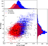 |
Fig. 1. CMD of the final sample of F (blue) and 1O (red) SMC Cepheids. The objects discarded in our cleaning procedure are shown as crosses. The distributions of the intrinsic color (V − I)0 and absolute magnitude MI are shown in the upper and right subpanels, respectively. |
3. Instability strip borders
To achieve our goal of determining the intrinsic empirical boundaries of the IS, we had to account for any factors that could influence its width. Only after making these corrections could we ensure that our results are comparable to theoretical models. In Section 2, we describe the criteria used to exclude outliers from our sample. The most significant remaining factor is the impact of reddening uncertainties. These uncertainties increase color scatter among Cepheids, thereby widening the IS. We note that, while photometric uncertainty also affects the IS width, its impact is approximately one order of magnitude smaller.
We performed the same method introduced in Paper I (Section 3 therein) to obtain intrinsic IS edges. First, we binned the whole Cepheids sample by I-band absolute magnitude. Most bins contain 200 stars, while the faintest contain around 100. We then determined each bin’s initial blue and red IS edges by locating the 1st and 99th percentiles of the color distribution. We then shifted each Cepheid’s intrinsic color by a random value drawn from a normal distribution with a standard deviation equal to the measured color uncertainty. Such a procedure results in some of them falling outside the initial edges. Subsequently, we separately counted the number of Cepheids that fell behind the red and blue edges. We repeated this process 10000 times and computed the median of the distribution of these numbers, namely nblue, nred. The final blue and red IS positions of each bin were obtained by moving the initial edges inward the IS by nblue and nred stars, respectively.
The Cepheids in the SMC have lower mean reddening than those in the LMC. In the LMC, the sample-average reddening is approximately 0.12 mag, whereas in the SMC it is 0.06 mag. Nevertheless, the reddening map from Skowron et al. (2021) shows similar average uncertainties of about 0.06 mag for both galaxies. This means that for the LMC and SMC, the effect of the IS widening due to the inaccurate dereddening of the sample, which affects the IS topology as discussed in Section 4.1, should be comparable.
The computed IS, including F and 1O Cepheids, are shown in Fig. 2 as red circles. Additionally, the median intrinsic colors (V − I)0 of each sample bin are shown as black circles. In this figure and throughout this paper, the periods of the 1O Cepheids were fundamentalized using equation (1c)2 in Pilecki (2024) and we overplotted constant period lines for 1, 3, and 10 days. These lines were calculated using the period-luminosity-color (PLC) relation computed using the I-band absolute magnitude and intrinsic color of the sample, and the periods provided in the OGLE catalog. Similar to our results in Paper I, we observe a change in slope of the calculated edges between faint and bright Cepheids close to the three-day constant period line. This change can also be noticed in the median intrinsic color along the IS (hereafter, median IS). To determine the break position in the IS edges, we use piecewise regression analysis (Muggeo 2003) implemented in Python by Pilgrim (2021). This technique employs a statistical hypothesis test to assess the significance of the break by testing whether at least one breakpoint exists against the null hypothesis of no breakpoints. We checked every fit of the IS boundaries, and in all cases the null hypothesis was rejected at a significance level below 1% (i.e., the probability of observing the data if the null hypothesis were true is below 1%). A larger number of breakpoints was not necessary; therefore, to describe the blue and red IS edges, we chose the model composed of two segments. Nevertheless, we kept the simplified wedge-shaped IS model (with no breaks) for comparison. Both IS models are shown in Fig. 2 and the coefficients of the fitted edges with 1-sigma uncertainties are listed in the Appendix (Table A.1). We emphasize that the wedge-shaped IS is just a crude approximation that has significant systematic deviations from the determined IS shape. Therefore, its formally determined uncertainties are not statistically meaningful, and are not provided. A discussion about the possible origin of the identified breaks can be found in Section 4.1.
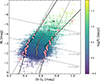 |
Fig. 2. CMD of F and 1O SMC Cepheids. The boundaries of our empirical IS are shown as red empty circles. The median intrinsic colors of each bin are shown as black empty circles. The upper and lower parts of the fitted red and blue edges are shown as black solid lines. The edges of the wedge-shaped IS are shown as dotted lines. The periods for these stars are shown with a color gradient. For 1O Cepheids, periods were fundamentalized. The overplotted dashed lines represent constant periods. |
Apart from the IS for the full sample, we also determined its edges separately for F and 1O Cepheids. The borders obtained for these subsamples are shown in Fig. 3 as red empty circles. Changes in the IS edge slope were detected in both sets, although at different pulsation periods compared with each other and with the full sample. As before, we fitted and presented in the figure both the two-segment linear models and a wedge-shaped IS. The corresponding coefficients for the IS edges are given in Table A.1.
4. Discussion
4.1. Topology of the IS boundaries in (V-I) color
Previous studies have reported breaks in the P-L relation of F and 1O Cepheids in the Magellanic Clouds. Bauer et al. (1999) noticed a slope change in the P-L relation for the SMC F Cepheids with periods shorter than two days, which was later confirmed by Sharpee et al. (2002), and Sandage et al. (2009). In a recent detailed analysis, Kurbah et al. (2025) identified multiple breaks in the period-amplitude, P-L, and amplitude-color relations of both F and FO Cepheids in the Magellanic Clouds. One of these breaks is located at a pulsation period of 2.5 days, which is close to the findings of previous studies. As shown graphically by Madore & Freedman (1991), the IS edges and the P-L relation are projections of the PLC relation onto the log L versus log T, and the log L versus log P plane, respectively. Therefore, features observed in one of these projections may also be visible in the others.
We observe changes in the slopes of the IS for our full sample, and also in the individual samples of F and 1O Cepheids. For our full sample, the break occurs at fundamentalized periods of around 2.5 days, specifically at absolute I-band magnitudes of −3.08 mag and −2.59 mag for the blue and red edges, respectively. This is similar to what we found for the LMC in Paper I, and consistent with the findings of Kurbah et al. (2025). On the other hand, for the individual F and 1O samples, we found changes in the slopes of the blue and red edges of the IS at different pulsation periods. For 1O Cepheids, the blue edge shows a break at a pulsation period of around 2 days (fundamentalized). However, the red edge shows the same feature at a shorter period of around 1.4 days (fundamentalized). The locations of these breaks in I-band absolute magnitude are −2.74 mag and −2.13 mag for the blue and red edge, respectively. In the case of F Cepheids, their blue edge shows a change in slope at a pulsating period of around 2 days, meanwhile, the red edge shows the same feature at around 3 days, similar to the full sample, which is expected since the red edge of the entire sample is dominated by F Cepheids, as seen in Fig. 1. These breaks are located at −2.59 and −3.38 I-band absolute magnitudes. Similar conclusions can be drawn for each sample when tracing the median along the IS. For the full sample, the break in the median IS is around 2.5 days, while for the F and 1O subsamples, the change in slope occurs between the breaks at the blue and red edges for a given pulsation mode. This indicates that the position of the break shifts gradually as we move from one edge to another.
In Paper I, we describe a break in the IS boundaries for LMC Cepheids with periods of around 3 days. A possible explanation for this feature is the depopulation of second and third-crossing Cepheids in the faint part of the IS. Since the extension of the blue loops decreases as the mass and period of Cepheids decrease, low-mass Cepheids would spend less time inside the IS, or they would not enter at all. This implies that Cepheids fainter than the break are likely on their first crossing of the IS. To test if the depopulation scenario could also produce features in the IS of the SMC, we used the stellar evolution code MESA (version r22.11.1) to calculate evolutionary tracks for nonrotating stars covering the mass range from 2 to 7 M⊙ in steps of 0.1 M⊙. The lower end of this mass range was extended, compared to the one used in Paper I, to consider all low-mass tracks that still crossed entirely or partially the SMC IS. We adopted Z = 0.001, 0.002, and 0.003 as representative metallicities for SMC stars (Choudhury et al. 2018). These tracks assume the solar mixture from Grevesse & Sauval (1998). We use a solar-calibrated mixing length parameter of αmlt = 1.9. For the convective boundaries, we use the predictive mixing scheme described in Paxton et al. (2018). Smolec et al. (2023) studied the behavior of blue loops as a function of core and envelope overshooting. They showed that the larger the envelope overshooting, the longer the blue loop. Based on this and after exploring parameters, we considered the exponential core and envelope overshooting with parameters f = 0.015 and f = 0.024, respectively. For this set of parameters, the extension of the blue loops qualitatively matches the observed IS, in particular, the resulting blue loops completely cross the IS. To account for mass loss during the evolution on the red giant branch (RGB), we use the Reimers (1975) prescription with a scaling factor ηR = 0.1.
The comparisons between evolutionary tracks and our empirical IS borders for the SMC (left panels) and LMC (Paper I, right panels) are shown in Fig. 4. In this figure, we show the extent of the blue loops (shaded areas) for each adopted metallicity. The tip of the RGB delimits these areas on the red side and the bluest extreme of the blue loop on the blue side. The upper limits are artificial and are defined by the evolutionary tracks for 7 M⊙-stars with different metallicities. Additionally, we show contours of the Cepheids’ density distributions of the 1O and F samples for both galaxies. The constant period lines were obtained independently for each galaxy. A discussion of the comparison between the SMC and LMC results can be found in Section 4.4.
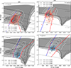 |
Fig. 4. CMD showing empirical IS edges (red empty circles) separately for SMC (left panels) and LMC (right panels) for 1O (upper panels) and F (lower panels) Cepheids. The black empty circles represent the median value of the intrinsic color of each bin of the corresponding sample. Fits for the blue and red edges, considering changes in slope at different pulsation periods, are shown as solid blue and red lines, respectively. Gray-shaded areas mark the blue loop extent (delimited by its bluest extreme and the tip of the RGB) for evolutionary tracks with representative Z for the SMC and LMC galaxies. The gray areas are created using tracks from 2 to 7 M⊙ for the SMC, and 3 to 7 M⊙ for the LMC. The upper limits for the areas are defined by the evolutionary tracks for 7 M⊙ and would extend farther up if tracks for higher masses were considered. |
In the case of the SMC, the model blue loops are particularly sensitive to metallicity, and their extensions vary in a more complex manner than in the LMC. For Z = 0.002 and 0.003, the extension “oscillates” around the IS as the mass of the star increases. For these models, the loops enter the IS at a Cepheid mass of 2.7 and 3.1 M⊙, respectively. These mass limits for blue loops are much lower than in the LMC (Paper I). Subsequently, their blue loop extension reaches a local maximum, gradually decreasing to a minimum extension at masses of 3.8 and 4.5 M⊙, respectively. We tried lower values of envelope overshoot, but the oscillatory effect was even more pronounced and the blue loops were clearly inconsistent with the data. On the other hand, the evolutionary tracks with Z = 0.001 show a more regular behavior since the extension of their blue loops increases as a function of stellar mass. These models enter the IS at a Cepheid mass of 2.3 M⊙, and their blue loops cover our F and 1O samples almost entirely.
The interpretation of results for the SMC is notably more intricate than that for the LMC due to a more complex influence of metallicity. Contrary to the LMC, the SMC model blue loops (except for Z = 0.003) cover almost completely the range of observed periods. This means that the depopulation scenario, which alters the slope of the IS, cannot be tested appropriately because the first and subsequent crossing Cepheids are mixed. However, the lower blue loop boundary for the highest metallicity correlates with the break for 1O Cepheids and the blue edge for F Cepheids. As the lower boundary for the lowest metallicity approaches the shortest periods in the sample, what we see as a change in slope may be an extended transition phase to a depopulated area. Such a transition phase is also present in the LMC, but because the lower blue loop boundaries for different Z values have a much smaller brightness spread, it is much tighter.
Another complication in interpreting the SMC data is the oscillation of the blue loop extensions mentioned above, which is absent in the LMC evolutionary tracks. This phenomenon suggests a significant decrease in the number of second- and third-crossing Cepheids with pulsation periods of around 3 to 10 days and a metallicity of Z = 0.003. This effect is not observed in our empirical results, which indicates there may be an issue with the choice of particular input physics that could affect blue loops in the evolutionary models. This effect has also been reported in the literature. As shown in Smolec et al. (2023), the extent of the blue loops shows nonlinear behavior as a function of mass for specific metallicity values and does not cross the IS for some masses (generally tracks with 4 or 5 M⊙). Furthermore, evolutionary tracks computed with the PARSEC v2.0 code (Costa et al. 2025), adopting a metallicity of Z = 0.002, and BaSTI (Hidalgo et al. 2018) tracks adopting Z = 0.003 show the same blue loop behavior. This could indicate that evolutionary models in general require fine-tuning for the loops at pulsation periods between 3 and 10 days to cross the IS. On the other hand, the distribution of metallicities of our Cepheids sample could be closer to lower metallicities than Z = 0.003. A more accurate understanding of the SMC metallicity distribution could let us better understand the IS’s topology.
4.2. Theoretical crossing times of the ISs
Using the evolutionary and pulsation models computed employing MESA and RSP, we estimated the expected number of Cepheids as a function of pulsation period, IS crossing, and metallicity, defined as
 (1)
(1)
where NF, 1O is the number of F and 1O Cepheids in our sample, and τF, 1O(P, Xing, Z) is the time that a Cepheid model with a pulsation period P and a metallicity Z spent inside a crossing (Xing) of our full-sample IS. The factor ξ(m)Δm is Salpeter (1955) initial mass function (IMF), where the dependency on mass was changed to dependency on period, using a period-mass relation computed from RSP models. This estimate assumes a constant star formation rate for the SMC. We compared the expected number of Cepheids with the observed number in our sample in Fig. 5 for the LMC (upper panels) and SMC (lower panels) galaxies. For this analysis, 1O periods were fundamentalized, as mentioned in Section 3.
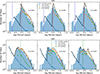 |
Fig. 5. Histogram of the number of LMC (upper panels) and SMC (lower panels) Cepheids, including F and 1O, as a function of fundamentalized pulsating period. The colored points show the expected number of Cepheids in each bin for different IS crossings, calculated using Eq. (1). The sum of the expected numbers of stars for all IS crossings is shown as a black solid line. The vertical blue, red, and green lines mark pulsation periods of 0.6 (the shortest period of our LMC models), 3, and 2.5 days, respectively. |
In the case of the LMC, the maximum of the Cepheid distribution is located at a pulsating period of 3 days. Then the number of stars gradually decreases as the period increases. For pulsating periods longer than 3 days, the expected number of Cepheids obtained for the second and third crossings is in good agreement with the observed number of stars. As mentioned in Paper I, for periods shorter than 3 days, the blue loops of our tracks do not cross the IS. Therefore, the expected number of short-period Cepheids drops significantly to only the first-crossing models. Since we computed evolutionary tracks starting from 2 M⊙, our results are limited to periods longer than 0.6 days, i.e., to the range in which the blue solid line in the upper panels of Fig. 5 is plotted.
A significant discrepancy between theoretical predictions and observations appears for Cepheids with pulsation periods shorter than 3 days. In the 1−3-day period range, the observed number of Cepheids decreases with period and, thus, with stellar mass. Conversely, theoretical models, primarily based on the first crossing of the IS, predict an increasing number of stars as the period shortens. This theoretical trend is influenced by two factors: a slower evolution rate for lower-mass stars, which increases their transit time across the IS, and the larger contribution of low-mass stars in the IMF.
Agreement between the expected and observed Cepheids is only achieved at a period of about 1 day. The observed excess of Cepheids between 1 and 3 days could potentially be explained by stars on a gradually narrowing blue loop that partially enter into the IS but do not cross it. However, current stellar evolution models fail to produce blue loops of sufficient extension to account for such objects in the LMC. An alternative scenario is that these Cepheids have lower metallicity than assumed in our models, as blue loops for more metal-poor stars may cross the IS at shorter periods.
For periods shorter than 1 day, the predicted number of Cepheids exceeds the observed number. For the shortest periods, however, the statistics of our sample are low, and the edges of the IS are poorly constrained (determined from only one sparsely populated bin). If all stars passing through the IS at a given brightness would pulsate, we would expect an increase in their number with decreasing mass (and shortening Cepheid period). Although some Cepheids exist in this zone, their number is much lower than predicted. This may indicate that, as mass decreases, the probability of exciting F or 1O pulsation modes decreases rapidly. On the other hand, this short-period region brings additional challenges for pulsation theory, which we use to determine the period of Cepheids passing the IS. Pulsation models presented by Buchler (2009, and references therein) showed that these short-period Cepheids present multi-mode pulsations (F/1O or involving higher overtones), together with hysteresis (i.e., the pulsational state depends on the evolutionary path). In such cases, determining the final pulsation mode and period requires nonlinear calculations that might alter the expected period distribution of Cepheids shown in Fig. 5. Nevertheless, such an analysis is beyond the scope of this paper.
In the case of the SMC galaxy, the peak of the Cepheid distribution occurs at significantly shorter periods than in the LMC, at around 1.4 days. There is close agreement between the observed and expected numbers of Cepheids with periods longer than 1 day, particularly for models with Z = 0.001. At higher metallicities, the expected number of stars differs from the observed number, likely due to the complex behavior of theoretical blue loops at such metallicities. Notably, the models for Z = 0.001 also successfully reproduce the observed Cepheid counts in the 1−3-day period range, whereas for the LMC, substantial disagreement was observed in that range across all considered values of Z.
Although for the SMC, better agreement is obtained for Z = 0.001, this does not mean its average metallicity is that low, as differences for this property between observations and theory for Cepheids are quite common (see, e.g., Taormina et al. 2018; Deka et al. 2025). Our theoretical value is still quite close to the one indicated by empirical studies, which is closer to Z = 0.002 (Breuval et al. 2024). Actually, our data could help calibrate theoretical models in terms of metallicity.
For periods shorter than 1 day, the expected number of stars differs significantly from the observed one. Given the low number of observed Cepheids in this period range, the same factors that produce such discrepancies for the LMC can apply to the SMC.
4.3. The geometry of the SMC
As shown by Jacyszyn-Dobrzeniecka et al. (2016), Cepheids trace an elongated shape along the line of sight of the SMC galaxy, covering a distance range between 50 and 80 kpc. This can increase the uncertainties in distance determinations for these objects, potentially affecting their positions in the CMD and, in turn, the IS shape. To mitigate this effect, we adopted the refined planar model by Breuval et al. (2024) to correct the distance to each Cepheid. Despite applying this procedure, we explored whether the spatial distribution of the SMC Cepheids could still affect the shape of the IS borders.
In Fig. 6, we show our full sample of Cepheids colored by their angular distance to the SMC center at  from Ripepi et al. (2017). Superimposed, we compare the IS edges of the full sample with those determined for a subsample of central Cepheids located within 0.6 deg from the SMC center. For clarity, here we join the points of the determined IS edges. Interestingly, these central Cepheids tend to be redder than those located farther away. The red edge is slightly, but systematically, shifted toward redder colors. For the blue edge, this depends on the luminosity: for fainter Cepheids, the difference is significant, but for brighter ones it decreases to zero.
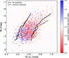 |
Fig. 6. CMD of F and 1O SMC Cepheids. The angular separation of Cepheids from the SMC center |

An inspection of the samples showed the mean intrinsic color uncertainties (which are dominated by the reddening uncertainties) are higher for central Cepheids compared to the complete sample, by 0.02 mag. Although this difference is significant, it should not ultimately affect the positions of the determined intrinsic edges. As mentioned in Section 3, higher uncertainties may indeed lead to a wider IS, but our correction procedure should return it to its original state. Moreover, any residual effect could leave the IS either slightly narrower or wider, but not shifted, and not by the observed amount. Although, in principle, the edges can also be affected by the uncertainty of the distance correction for Cepheids located farther from the center, we also do not expect it to result in a systematic shift in color.
The observed shift to redder colors may indicate that central Cepheids are more metal-rich than the average metallicity. Recently, Murray et al. (2024) showed that the SMC is composed of two substructures with different chemical compositions, separated by 5 kpc along the line of sight. Nevertheless, the difference in metallicity within their sample of stars is relatively small, and it is unlikely that it would be responsible for the shifts in the IS edges that we have observed. Another possibility for shifting the whole IS to redder colors is an additional reddening for the central Cepheids, which is not accounted for in the reddening maps we used. This is quite likely, as the procedure used by Skowron et al. (2021) is calibrated in the galaxy’s outer regions.
Actually, with the above test, we intended to check whether the IS for central Cepheids would be slightly narrower due to lower geometrical corrections to the absolute magnitudes. This, however, is not unambiguously observed.
4.4. Comparison with the LMC ISs
A source of uncertainty in the cosmic distance ladder that is still debated is the metallicity dependence of the P-L relations of classical Cepheids (see, e.g., Breuval et al. 2025; Khan et al. 2025). Using theoretical models, it was shown that metallicity affects the shape of the IS (Marconi et al. 2005), which, in turn, may alter the P-L relations (Madore & Freedman 1991). To study this effect empirically, we compare the ISs for F and 1O Cepheids in the LMC and SMC (Fig. 7). We included edges with breaks, in addition to the fitted median IS for both galaxies. The constant period lines shown in this figure are those computed for the SMC sample (they are slightly brighter than the same period lines calculated for the LMC). The following comparisons are based on the individual points of the IS boundaries and the mean values of the linear fits.
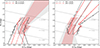 |
Fig. 7. Comparison of empirical ISs of the LMC (Paper I) and SMC (this work) in red and black, respectively. The dashed lines represent the middle of the ISs. The left panel compares only the ISs for 1O Cepheids, while the right panel shows F ISs. The shaded areas show the IS for F mode in the left panel and for 1O mode in the right panel, allowing comparison between the modes and illustrating their superposition. |
Taking into account the blue edge of 1O Cepheids and the red edge of F Cepheids, the IS for the LMC is narrower than for the SMC. The superposition of ISs for both pulsation modes (F and 10) is also narrower for the LMC. The breaks in slope and color of the ISs differ between the two galaxies considered, with those of the SMC occurring at shorter periods.
Regarding the IS for 1O Cepheids, the blue edge for the LMC is generally redder than the SMC, except for the longest periods. This is theoretically expected since more metal-rich pulsation models show redder IS borders. However, this explanation does not apply to the median and red edge of the empirical IS, which exhibit more complex behavior. For the LMC, both are bluer for periods longer than 3 days and shorter than 1 day. Between 1 and 2 days, the LMC median is redder, and the red edge is roughly consistent with that for the SMC. For the shortest periods, the difference between the two galaxies increases significantly, but this can be partly due to extrapolation. As mentioned in Section 4.2, this period range is poorly constrained due to low statistics of our sample below MI ∼ −1 mag (the faintest point for the SMC IS edge is located at MI = −1.5 mag).
For F Cepheids, the ISs for both galaxies are very similar, with the LMC IS being generally narrower compared to the SMC. The blue edge of the LMC IS is redder, and its red edge is bluer. The median LMC IS is very consistent with that of the SMC. This observed similarity in the ISs of F Cepheids of different metallicities is very fortunate for their use in distance determination. It minimizes the systematic error introduced when applying empirical relations to Cepheids in different environments. Based only on our current comparison, we can recommend using F Cepheids with periods longer than 3 days for distance determination. Given the dependence of the break position on metallicity and the lack of a similar analysis for Cepheids at solar metallicity, this period limit may be higher. Once we extend the comparison to higher-metallicity Cepheids, we will be able to provide a more accurate value.
The LMC blue edge is redder than the SMC blue edge, as expected from a theoretical perspective. However, the bluer color of the LMC red edge for F Cepheids is the opposite of expectations, and the similar color of the median ISs in both galaxies is also surprising. Further study will be needed to determine the cause of the discrepancy between theory and observation.
As an additional comparison, we fitted a P-L relation of the LMC and SMC samples. For the SMC, the P-L slope was fixed to the LMC value. We applied a shift to the intercept of the LMC P-L, which corresponds to the difference in distance modulus (DM) between the Magellanic clouds (δ DM = 0.5, Pietrzyński et al. 2019; Graczyk et al. 2020), to obtain the intercept of the SMC P-L. Using the PLC relation, we converted our empirical ISs (including their medians) to the period-luminosity plane and marked them as triangles (and circles). We then computed the residuals between the absolute I-band magnitudes and the P-L relations for each galaxy. These results are shown in Fig. 8. In this plane, it can be seen how the effect of metallicity on IS depends on pulsation period and position within the IS. It is important to note that several other physical effects, in addition to metallicity, contribute to the observed scatter in the P-L relation. These factors can include, among others, helium content, rotation, and geometrical corrections of the Magellanic Clouds (see, e.g., Marconi et al. 2005; Anderson et al. 2016; Breuval et al. 2022). In Fig. 8, it can be noted that, comparing SMC Cepheids near the red edge with LMC Cepheids near the blue edge can yield results that differ entirely from those obtained when comparing SMC Cepheids near the blue edge with LMC Cepheids near the red edge. Also, based on the median IS, the slope of the SMC relation differs from that for LMC. Although, on average, the shift between the two relations is consistent with the difference in distance moduli between the SMC and the LMC, the median values at distinct periods are considerably different. For example, using SMC Cepheids near log P = 0.2 versus those near log P = 0.6 would yield a systematic difference of 0.15 mag. In Khan et al. (2025), the difference in P-L intercepts between the SMC and Milky Way metallicities is generally smaller than ∼0.1 mag (see, e.g., Fig. 9 and Table B.1 of their work), therefore using SMC Cepheid samples with different average periods may significantly affect the slope of the metallicity dependence. For the I-band, the difference between the LMC and SMC P-L intercepts in Khan et al. (2025) ranges from 0.005 to 0.075 mag, depending on the pivot period, also indicating period dependence. Moreover, generally, the wider SMC IS results in higher scatter in the P-L relation across all pulsation periods.
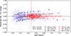 |
Fig. 8. Residuals between I-band absolute magnitudes of SMC and LMC F Cepheids and P-L relations for each galaxy, while maintaining the slope fixed to the value obtained for the LMC. In addition, the residuals of the IS edges of both LMC and SMC, as well as their corresponding median parts, are shown as red and black triangles and empty circles. The SMC and LMC median ISs are connected with black and red lines, respectively. The vertical red line marks a pulsation period of 3 days. |
Taking into account the samples’ locations within the instability strip may lead to a more accurate estimate of the metallicity dependence of the P-L relations. This can be done in two ways: either by selecting a sample representative of the IS part we want to study (with a proper distribution along the period and color axes), or by applying a sample-dependent correction for its position within the IS. Both procedures should allow for separating metallicity effects from other biases, homogenize results across different samples, and ultimately increase their accuracy.
4.5. Comparison with theoretical ISs
The theoretical IS edges have been extensively studied in the literature, exploring how various micro- and macrophysical effects alter the IS shape. Often, these studies provide the IS edges in the log Teff − log L plane; thus, converting our results to this plane is necessary for comparison.
Following the same procedure as in Paper I, each point of our IS for F Cepheids in the CMD plane was converted to the log Teff − log L plane using the color-temperature and bolometric correction calibration presented by Worthey & Lee (2011). The points were fitted in the same way as for the IS in the CMD. The coefficients of the empirical IS in the log Teff − log L plane are presented in Table A.2. In the following part of this section, we compared our two-part IS with literature results; thus, conclusions may differ between the lower and upper parts of our IS.
The theoretical ISs for F Cepheids presented by Anderson et al. (2016), and also used in Khan et al. (2025), are shown in Fig. 9. Their results were computed using the Geneva code of stellar evolution (Eggenberger et al. 2008), for different metallicities and rotation rates, and an extended version of the method described in Saio et al. (1983) to perform a linear non-adiabatic radial pulsation analysis. We compare our results with their ISs of Z = 0.002, and three rotation rates ω = 0.0, 0.5, and 0.9. We reproduced their IS boundaries based on the three crossings of the IS from their Table A.3, which provides the effective temperature and luminosity of models that enter or exit the IS for each mass. Similar to the comparison performed in Paper I for the LMC, their theoretical blue edge agrees remarkably well with the bright part of our empirical one. However, the faintest portion of our blue edge is systematically cooler. Regarding their red edge, its central part is similar to our empirical red edge; however, it deviates significantly for faintest and brightest Cepheids. As for rotation, our empirical results favor models with a high rotation rate, which is consistent with the conclusions for the LMC (see Paper I).
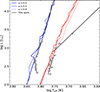 |
Fig. 9. Comparison of theoretical F ISs presented in Anderson et al. (2016) (blue and red) and our empirical IS (black lines and black points with white centers) in an HRD. The different line styles represent different rotation rates ω, expressed as a fraction of critical velocity on ZAMS. |
In Fig. 10, we compare our results with the theoretical IS for F Cepheids computed by De Somma et al. (2022) with a metallicity of Z = 0.004. Their nonlinear pulsational analysis was performed using the Stellingwerf code (Stellingwerf 1982) with updated opacity tables. Their nonlinear pulsation calculations approximate the effects of overshooting by considering an increase in the luminosity, over their canonical models (case A), of Δ(log L/L⊙) = 0.2 dex (case B), and Δ(log L/L⊙) = 0.4 dex (case C). Additionally, they consider three values for the superadiabatic convection efficiency of αml = 1.5, αml = 1.7, and αml = 1.9. We note good agreement for the blue edge, considering their case C, and αml = 1.7 and αml = 1.9. In the case of the red edge, our results globally align closer to their borders with the lowest αml, and case B. Quite a good agreement is also obtained for the central part for αml = 1.7 and case B.
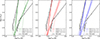 |
Fig. 10. Comparison of theoretical F ISs for Z = 0.004 presented in De Somma et al. (2024) and our empirical IS (black lines and black points with white centers) in an HRD. From left to right, the superadiabatic convection efficiency αml of their models increases. In addition, the different line styles represent different increases of the luminosity applied by the authors to their canonical model. |
For theoretical ISs of De Somma et al. (2022), the agreement of the red edge with our empirical one is better than for the red edge of Anderson et al. (2016). In particular, a χ2 calculated between the red edge considering αml = 1.5 and case B from De Somma et al. (2022) and our empirical red edge, is 28% lower than the one obtained considering ω = 0.9 from Anderson et al. (2016). This result is expected since the location of the red edge depends on the interplay between pulsation and convection, the latter quenching pulsation, which is better described by nonlinear pulsational calculations. These nonlinear models of De Somma et al. (2022) also show a gradual diminishing of the IS in the faintest part, which may support our aforementioned observation of the rapidly decreasing number of Cepheids with the shortest periods.
More recently, Deka et al. (2024) studied the effects on the IS using different sets of convective parameters in RSP. These parameters can be found in Table 4 of Paxton et al. (2019), from set A to set D, increasing the complexity of the convective modeling with each consecutive set. The set A represents the simplest convective model; set B considers radiative cooling; set C takes into account turbulent pressure and turbulent flux; and set D adds all the previous effects simultaneously. A comparison between our results for 1O and F Cepheids with those obtained by Deka et al. (2024) is shown in Fig. 11. We observed good agreement between our blue edges and their results for both samples, considering their set B. In the case of our red edge, it appears to be closer to their results using sets A and B. Contrary to the LMC case (Paper I), the RSP set D does not show satisfactory agreement with our empirical results. The latter highlights the complex interplay between metallicity and convection in the calculation of theoretical ISs.
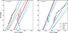 |
Fig. 11. Comparison of theoretical ISs for Z = 0.002 presented in Deka et al. (2024) and our empirical IS (black lines and black points with white centers) in a CMD. The ISs of 1O Cepheids are shown in the left panel, while ISs of F Cepheids are shown in the right panel. The different colors represent the sets of RSP convective parameters considered by the authors. |
5. Conclusions
We used a sample of SMC Cepheids from the OGLE-IV catalog to compute the empirical, intrinsic IS. We determined the IS edges for F and 1O Cepheids, together and separately, using I and V bands. In all cases, a change of slope of the IS was observed at pulsating periods between 1.4 and 3 days. The break is most prominent in the red edges, but it is also easily noticeable in the median IS.
Using a grid of evolutionary tracks computed with the stellar evolution code MESA, we investigated the connection between the observed shape of the IS and the evolution of intermediate-mass stars. Our results showed that the metallicity of the evolutionary tracks strongly influences the behavior of the blue loops. While some of this behavior coincides with observed changes in the IS (e.g., the red edge of the 1O IS), the oscillatory behavior of the blue loops does not produce observable changes in the IS’ shape. This indicates that this complex feature of our models is most likely due to the physical input parameters, rather than a physical process within the star. More detailed studies of this phenomenon should be conducted to improve our understanding of Cepheids with low metallicity.
For the SMC, the lower mass limit at which the blue loops enter the IS is low enough to cover our entire Cepheid sample. This means that the first and subsequent crossing Cepheids are mixed, and depopulation cannot explain any significant change in the shape of the IS, as we proposed in Paper I for the LMC, unless we reject the models with lower metallicity. However, for both galaxies, the break also coincides with the effect of the metallicity gradient on the lower blue loop boundary. In the LMC, the transition phase between the lower and upper parts of the IS is narrow in luminosity, whereas in the SMC it is broader and can be treated as a separate component with a different slope. Therefore, the metallicity gradient can be another factor responsible for shaping the IS in a given galaxy.
We performed a more detailed comparison between our theoretical and empirical results by calculating the expected number of Cepheids as a function of period, based on the IS crossing time of our evolutionary tracks. In the case of the LMC, we found close agreement between the expected and observed numbers of Cepheids with pulsating periods longer than 3 days. On the contrary, for shorter periods (between 1 and 3 days), our evolutionary tracks are not able to reproduce enough second and third crossing Cepheids to match the observed number of stars. This may indicate a problem with theoretical models in this range, which do not produce sufficiently extended blue loops for lower-mass stars. For periods shorter than 1 day, the expected number of stars is larger than the observed one. On the other hand, the SMC results showed close agreement between empirical and theoretical results for pulsating periods as short as 1 day. For shorter periods, the expected number of stars is much larger than the observed number, which is likely related to a problem in our linear pulsating models and the extrapolation of our empirical IS where the statistics are low. Generally, the results for both galaxies indicate that short-period Cepheids remain a modeling challenge for current stellar evolution codes. A similar conclusion, although for other reasons, was drawn in our recent study of a short-period binary Cepheid OGLE LMC-CEP-1347 (Espinoza-Arancibia & Pilecki 2025). The analysis of this and other binary Cepheids also indicates that the number of short-period Cepheids can be affected by merger origin from lower-mass stars (Pilecki et al. 2022, 2024).
The elongated geometry of the SMC poses an additional challenge for the detailed study of the IS, as it increases the uncertainty in the calculated distances to Cepheids. To study its impact on the shape of the IS, we applied our method to a subsample of Cepheids near the center of the SMC. We report a significant shift of the blue edge of the IS to cooler temperatures. This effect is also observed at the red edge, but to a lesser extent. A possible explanation is that this subsample of Cepheids shows higher reddening than indicated by the reddening maps. Additionally, a shift to redder colors can be explained by a higher metallicity than in the full sample. The latter is consistent with previous studies, although the magnitude of this effect remains uncertain.
To test the effect of metallicity on the IS, we compared our empirical results for the SMC and LMC. The SMC showed a wider IS for both pulsating modes. Furthermore, the blue edges in both galaxies follow the expected theoretical trend: the more metal-rich LMC blue edge is redder than its SMC counterpart. The red edge, on the other hand, presents a more complex behavior. Its position is strongly influenced by changes in slope at different luminosities, and it displays a metallicity dependence opposite to theoretical predictions. This implies that accurately locating a Cepheid sample within the IS is crucial for precisely determining the metallicity dependence in P-L relations. In particular, selecting Cepheids located in different parts of the IS could yield different determined metallicity effects. On the other hand, the transition of 1O to F Cepheids, delimited by the red edge of the 1O IS and the blue edge of the F IS, does present a complex dependence on metallicity. This could be further explored by studying the precise location of double-mode Cepheids in a CMD, which may be switching between F and 1O pulsation modes. An important conclusion from the comparison of ISs for the LMC and SMC is that, within this metallicity range, F Cepheids with periods longer than 3 days should be relatively safe for distance determination. However, at higher metallicities, there is no similar analysis. In the future, we will extend our study to higher metallicities (e.g., in the Milky Way) and provide a precise recommendation considering this environment.
We compared our empirically determined IS with prior theoretical studies. The bright part of the F blue edge of Anderson et al. (2016) shows good agreement with our empirical IS, while the bright end of their F red edge deviates from it significantly. The edges obtained in De Somma et al. (2022) can reproduce our IS well, but no unique combination of their parameters can reproduce both red and blue edges. Our blue edge is closer to their Case C, considering moderate and high convection efficiency (αml = 1.7 and αml = 1.9). On the other hand, our red edge agrees better with their results for Case B and low convection efficiency (αml = 1.5). In the case of the results by Deka et al. (2024), only our blue edge can be reproduced satisfactorily, in particular using their set B (for both 1O and F Cepheids), or their set A (only F Cepheids). The slopes of our red edge cannot be reproduced by their results.
Our study of the instability strip in the Magellanic Clouds demonstrates its value for future Cepheid research. This includes, among others, constraining theoretical evolutionary and pulsational models, investigating the behavior of short-period Cepheids, and understanding the role of metallicity in shaping the relation between the period, luminosity, and color of Cepheids. Furthermore, these IS edges can be applied to other low-metallicity environments with fewer stars to efficiently identify and select Cepheids, also depending on their pulsation mode.
Data availability
Data points describing the IS edges in a machine-readable form are available at https://doi.org/10.5281/zenodo.17277341
Acknowledgments
We thank the anonymous referee for the constructive comments and suggestions. We acknowledge support from the Polish National Science Center grant SONATA BIS 2020/38/E/ST9/00486. This research has made use of NASA’s Astrophysics Data System Service.
References
- Anderson, R. I., Saio, H., Ekström, S., Georgy, C., & Meynet, G. 2016, A&A, 591, A8 [NASA ADS] [CrossRef] [EDP Sciences] [Google Scholar]
- Bauer, F., Afonso, C., Albert, J. N., et al. 1999, A&A, 348, 175 [NASA ADS] [Google Scholar]
- Bono, G., Braga, V. F., & Pietrinferni, A. 2024, A&ARv, 32, 4 [Google Scholar]
- Breuval, L., Riess, A. G., Kervella, P., Anderson, R. I., & Romaniello, M. 2022, ApJ, 939, 89 [NASA ADS] [CrossRef] [Google Scholar]
- Breuval, L., Riess, A. G., Casertano, S., et al. 2024, ApJ, 973, 30 [Google Scholar]
- Breuval, L., Anand, G. S., Anderson, R. I., et al. 2025, ArXiv e-prints [arXiv:2507.15936] [Google Scholar]
- Buchler, J. R. 2009, AIP Conf. Ser., 1170, 51 [Google Scholar]
- Catelan, M., & Smith, H. A. 2015, Pulsating Stars (Weinheim: Wiley-VCH) [Google Scholar]
- Choudhury, S., Subramaniam, A., Cole, A. A., & Sohn, Y. J. 2018, MNRAS, 475, 4279 [NASA ADS] [CrossRef] [Google Scholar]
- Costa, G., Shepherd, K. G., Bressan, A., et al. 2025, A&A, 694, A193 [NASA ADS] [CrossRef] [EDP Sciences] [Google Scholar]
- De Somma, G., Marconi, M., Molinaro, R., et al. 2022, ApJS, 262, 25 [NASA ADS] [CrossRef] [Google Scholar]
- De Somma, G., Marconi, M., Cassisi, S., & Molinaro, R. 2024, ApJ, 977, 1 [Google Scholar]
- Deka, M., Bellinger, E. P., Kanbur, S. M., et al. 2024, MNRAS, 530, 5099 [Google Scholar]
- Deka, M., Ahlborn, F., Braun, T. A. M., & Weiss, A. 2025, A&A, 699, A351 [NASA ADS] [CrossRef] [EDP Sciences] [Google Scholar]
- Eggenberger, P., Meynet, G., Maeder, A., et al. 2008, Ap&SS, 316, 43 [Google Scholar]
- Espinoza-Arancibia, F., & Pilecki, B. 2025, ApJ, 981, L35 [Google Scholar]
- Espinoza-Arancibia, F., Catelan, M., Hajdu, G., et al. 2022, MNRAS, 517, 1538 [Google Scholar]
- Espinoza-Arancibia, F., Pilecki, B., Pietrzyński, G., Smolec, R., & Kervella, P. 2024, A&A, 682, A185 [NASA ADS] [CrossRef] [EDP Sciences] [Google Scholar]
- Fernie, J. D. 1990, ApJ, 354, 295 [NASA ADS] [CrossRef] [Google Scholar]
- Graczyk, D., Pietrzyński, G., Thompson, I. B., et al. 2020, ApJ, 904, 13 [Google Scholar]
- Grevesse, N., & Sauval, A. J. 1998, Space Sci. Rev., 85, 161 [Google Scholar]
- Hidalgo, S. L., Pietrinferni, A., Cassisi, S., et al. 2018, ApJ, 856, 125 [Google Scholar]
- Hocdé, V., Smolec, R., Moskalik, P., Singh Rathour, R., & Ziółkowska, O. 2024, A&A, 683, A233 [NASA ADS] [CrossRef] [EDP Sciences] [Google Scholar]
- Jacyszyn-Dobrzeniecka, A. M., Skowron, D. M., Mróz, P., et al. 2016, Acta Astron., 66, 149 [NASA ADS] [Google Scholar]
- Jermyn, A. S., Bauer, E. B., Schwab, J., et al. 2023, ApJS, 265, 15 [NASA ADS] [CrossRef] [Google Scholar]
- Khan, S., Anderson, R. I., Ekström, S., Georgy, C., & Breuval, L. 2025, A&A, 702, A235 [NASA ADS] [CrossRef] [EDP Sciences] [Google Scholar]
- Kurbah, K., Kanbur, S. M., Deb, S., et al. 2025, MNRAS, 541, 2594 [Google Scholar]
- Madore, B. F., & Freedman, W. L. 1991, PASP, 103, 933 [Google Scholar]
- Madore, B. F., Freedman, W. L., & Moak, S. 2017, ApJ, 842, 42 [NASA ADS] [CrossRef] [Google Scholar]
- Marconi, M., Musella, I., & Fiorentino, G. 2005, ApJ, 632, 590 [Google Scholar]
- Marconi, M., De Somma, G., Molinaro, R., et al. 2024, MNRAS, 529, 4210 [NASA ADS] [CrossRef] [Google Scholar]
- Muggeo, V. M. R. 2003, Stat. Med., 22, 3055 [Google Scholar]
- Murray, C. E., Hasselquist, S., Peek, J. E. G., et al. 2024, ApJ, 962, 120 [NASA ADS] [CrossRef] [Google Scholar]
- Paxton, B., Bildsten, L., Dotter, A., et al. 2011, ApJS, 192, 3 [Google Scholar]
- Paxton, B., Cantiello, M., Arras, P., et al. 2013, ApJS, 208, 4 [Google Scholar]
- Paxton, B., Marchant, P., Schwab, J., et al. 2015, ApJS, 220, 15 [Google Scholar]
- Paxton, B., Schwab, J., Bauer, E. B., et al. 2018, ApJS, 234, 34 [NASA ADS] [CrossRef] [Google Scholar]
- Paxton, B., Smolec, R., Schwab, J., et al. 2019, ApJS, 243, 10 [Google Scholar]
- Pel, J. W., & Lub, J. 1978, in The HR Diagram – The 100th Anniversary of Henry Norris Russell, eds. A. G. D. Philip, & D. S. Hayes, 80, 229 [Google Scholar]
- Pietrzyński, G., Graczyk, D., Gallenne, A., et al. 2019, Nature, 567, 200 [Google Scholar]
- Pilecki, B. 2024, ApJ, 970, L14 [NASA ADS] [CrossRef] [Google Scholar]
- Pilecki, B., Pietrzyński, G., Anderson, R. I., et al. 2021, ApJ, 910, 118 [NASA ADS] [CrossRef] [Google Scholar]
- Pilecki, B., Thompson, I. B., Espinoza-Arancibia, F., et al. 2022, ApJ, 940, L48 [NASA ADS] [CrossRef] [Google Scholar]
- Pilecki, B., Thompson, I. B., Espinoza-Arancibia, F., et al. 2024, A&A, 686, A263 [NASA ADS] [CrossRef] [EDP Sciences] [Google Scholar]
- Pilgrim, C. 2021, J. Open Source Softw., 6, 3859 [NASA ADS] [CrossRef] [Google Scholar]
- Reimers, D. 1975, Mem. Soc. Roy. Sci. Liege, 8, 369 [Google Scholar]
- Ripepi, V., Cioni, M.-R. L., Moretti, M. I., et al. 2017, MNRAS, 472, 808 [Google Scholar]
- Saio, H., Winget, D. E., & Robinson, E. L. 1983, ApJ, 265, 982 [Google Scholar]
- Salpeter, E. E. 1955, ApJ, 121, 161 [Google Scholar]
- Sandage, A., Tammann, G. A., & Reindl, B. 2004, A&A, 424, 43 [NASA ADS] [CrossRef] [EDP Sciences] [Google Scholar]
- Sandage, A., Tammann, G. A., & Reindl, B. 2009, A&A, 493, 471 [NASA ADS] [CrossRef] [EDP Sciences] [Google Scholar]
- Schlegel, D. J., Finkbeiner, D. P., & Davis, M. 1998, ApJ, 500, 525 [Google Scholar]
- Sharpee, B., Stark, M., Pritzl, B., et al. 2002, AJ, 123, 3216 [NASA ADS] [CrossRef] [Google Scholar]
- Skowron, D. M., Skowron, J., Udalski, A., et al. 2021, ApJS, 252, 23 [Google Scholar]
- Smolec, R., & Moskalik, P. 2008, Acta Astron., 58, 193 [NASA ADS] [Google Scholar]
- Smolec, R., Ziolkowska, O., Rathour, R. S., & Hocde, V. 2023, PLATO Stellar Science Conference, 2023, 7 [Google Scholar]
- Soszyński, I., Udalski, A., Szymański, M. K., et al. 2017, Acta Astron., 67, 103 [NASA ADS] [Google Scholar]
- Stellingwerf, R. F. 1982, ApJ, 262, 330 [NASA ADS] [CrossRef] [Google Scholar]
- Stuck, M., Pratt, J., Baraffe, I., et al. 2025, A&A, 698, A304 [NASA ADS] [CrossRef] [EDP Sciences] [Google Scholar]
- Tammann, G. A., Sandage, A., & Reindl, B. 2003, A&A, 404, 423 [NASA ADS] [CrossRef] [EDP Sciences] [Google Scholar]
- Taormina, M., Pilecki, B., & Smolec, R. 2018, in The RR Lyrae 2017 Conference. Revival of the Classical Pulsators: from Galactic Structure to Stellar Interior Diagnostics, eds. R. Smolec, K. Kinemuchi, & R. I. Anderson, 6, 325 [Google Scholar]
- Turner, D. G. 2001, Odessa Astron. Publ., 14, 166 [NASA ADS] [Google Scholar]
- Walmswell, J. J., Tout, C. A., & Eldridge, J. J. 2015, MNRAS, 447, 2951 [NASA ADS] [CrossRef] [Google Scholar]
- Worthey, G., & Lee, H. 2011, ApJS, 193, 1 [Google Scholar]
- Xu, H. Y., & Li, Y. 2004, A&A, 418, 213 [NASA ADS] [CrossRef] [EDP Sciences] [Google Scholar]
- Zhao, L., Song, H., Meynet, G., et al. 2023, A&A, 674, A92 [NASA ADS] [CrossRef] [EDP Sciences] [Google Scholar]
- Ziółkowska, O., Smolec, R., Thoul, A., et al. 2024, ApJS, 274, 30 [CrossRef] [Google Scholar]
We considered AI/AV = 0.594, and E(V − I) = 1.238 E(B − V).
PF/P1O = 1.356 + 0.068log P1O.
Appendix A: Tables with coefficients of the red and blue edges of the IS
Coefficients of the red and blue edges of the IS in the color–magnitude plane.
Coefficients of the red and blue edges of the IS in the temperature–luminosity plane.
All Tables
Coefficients of the red and blue edges of the IS in the color–magnitude plane.
Coefficients of the red and blue edges of the IS in the temperature–luminosity plane.
All Figures
|
Fig. 1. CMD of the final sample of F (blue) and 1O (red) SMC Cepheids. The objects discarded in our cleaning procedure are shown as crosses. The distributions of the intrinsic color (V − I)0 and absolute magnitude MI are shown in the upper and right subpanels, respectively. |
| In the text | |
|
Fig. 2. CMD of F and 1O SMC Cepheids. The boundaries of our empirical IS are shown as red empty circles. The median intrinsic colors of each bin are shown as black empty circles. The upper and lower parts of the fitted red and blue edges are shown as black solid lines. The edges of the wedge-shaped IS are shown as dotted lines. The periods for these stars are shown with a color gradient. For 1O Cepheids, periods were fundamentalized. The overplotted dashed lines represent constant periods. |
| In the text | |
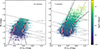 |
Fig. 3. Same as Fig. 2, but independently for 1O (left panel) and F (right panel) Cepheids. |
| In the text | |
|
Fig. 4. CMD showing empirical IS edges (red empty circles) separately for SMC (left panels) and LMC (right panels) for 1O (upper panels) and F (lower panels) Cepheids. The black empty circles represent the median value of the intrinsic color of each bin of the corresponding sample. Fits for the blue and red edges, considering changes in slope at different pulsation periods, are shown as solid blue and red lines, respectively. Gray-shaded areas mark the blue loop extent (delimited by its bluest extreme and the tip of the RGB) for evolutionary tracks with representative Z for the SMC and LMC galaxies. The gray areas are created using tracks from 2 to 7 M⊙ for the SMC, and 3 to 7 M⊙ for the LMC. The upper limits for the areas are defined by the evolutionary tracks for 7 M⊙ and would extend farther up if tracks for higher masses were considered. |
| In the text | |
|
Fig. 5. Histogram of the number of LMC (upper panels) and SMC (lower panels) Cepheids, including F and 1O, as a function of fundamentalized pulsating period. The colored points show the expected number of Cepheids in each bin for different IS crossings, calculated using Eq. (1). The sum of the expected numbers of stars for all IS crossings is shown as a black solid line. The vertical blue, red, and green lines mark pulsation periods of 0.6 (the shortest period of our LMC models), 3, and 2.5 days, respectively. |
| In the text | |
|
Fig. 6. CMD of F and 1O SMC Cepheids. The angular separation of Cepheids from the SMC center |
| In the text | |
|
Fig. 7. Comparison of empirical ISs of the LMC (Paper I) and SMC (this work) in red and black, respectively. The dashed lines represent the middle of the ISs. The left panel compares only the ISs for 1O Cepheids, while the right panel shows F ISs. The shaded areas show the IS for F mode in the left panel and for 1O mode in the right panel, allowing comparison between the modes and illustrating their superposition. |
| In the text | |
|
Fig. 8. Residuals between I-band absolute magnitudes of SMC and LMC F Cepheids and P-L relations for each galaxy, while maintaining the slope fixed to the value obtained for the LMC. In addition, the residuals of the IS edges of both LMC and SMC, as well as their corresponding median parts, are shown as red and black triangles and empty circles. The SMC and LMC median ISs are connected with black and red lines, respectively. The vertical red line marks a pulsation period of 3 days. |
| In the text | |
|
Fig. 9. Comparison of theoretical F ISs presented in Anderson et al. (2016) (blue and red) and our empirical IS (black lines and black points with white centers) in an HRD. The different line styles represent different rotation rates ω, expressed as a fraction of critical velocity on ZAMS. |
| In the text | |
|
Fig. 10. Comparison of theoretical F ISs for Z = 0.004 presented in De Somma et al. (2024) and our empirical IS (black lines and black points with white centers) in an HRD. From left to right, the superadiabatic convection efficiency αml of their models increases. In addition, the different line styles represent different increases of the luminosity applied by the authors to their canonical model. |
| In the text | |
|
Fig. 11. Comparison of theoretical ISs for Z = 0.002 presented in Deka et al. (2024) and our empirical IS (black lines and black points with white centers) in a CMD. The ISs of 1O Cepheids are shown in the left panel, while ISs of F Cepheids are shown in the right panel. The different colors represent the sets of RSP convective parameters considered by the authors. |
| In the text | |
Current usage metrics show cumulative count of Article Views (full-text article views including HTML views, PDF and ePub downloads, according to the available data) and Abstracts Views on Vision4Press platform.
Data correspond to usage on the plateform after 2015. The current usage metrics is available 48-96 hours after online publication and is updated daily on week days.
Initial download of the metrics may take a while.