| Issue |
A&A
Volume 706, February 2026
|
|
|---|---|---|
| Article Number | A24 | |
| Number of page(s) | 15 | |
| Section | Extragalactic astronomy | |
| DOI | https://doi.org/10.1051/0004-6361/202557085 | |
| Published online | 27 January 2026 | |
ODIN: Using multiplicity of Lyman-alpha emitters to assess star formation activity in dark matter halos
1
Instituto de Astronomía Teórica y Experimental (IATE), CONICET-UNC Laprida 854 X500BGR Córdoba, Argentina
2
Facultad de Matemática, Astronomía, Física y Computación, Universidad Nacional de Córdoba, Bvd. Medina Allende s/n Ciudad Universitaria X5000HU Córdoba, Argentina
3
Observatorio Astronómico de Córdoba, Universidad Nacional de Córdoba Laprida 854 X5000BGR Córdoba, Argentina
4
Department of Physics and Astronomy, Rutgers, the State University of New Jersey Piscataway NJ 08854, USA
5
Universidad Andres Bello, Facultad de Ciencias Exactas, Departamento de Fisica y Astronomia, Instituto de Astrofisica, Fernandez Concha 700 Las Condes Santiago RM, Chile
6
Department of Physics and Astronomy, Purdue University 525 Northwestern Avenue West Lafayette IN 47906, USA
7
Korea Institute for Advanced Study 85 Hoegi-ro Dongdaemun-gu Seoul 02455, Republic of Korea
8
Korea Astronomy and Space Science Institute, 776 Daedeokdae-ro Yuseong-gu Daejeon 34055, Republic of Korea
9
Department of Astronomy and Astrophysics, The Pennsylvania State University University Park PA 16803, USA
10
Institute for Gravitation and the Cosmos, The Pennsylvania State University University Park PA 16803, USA
11
Millennium Nucleus for Galaxies (MINGAL), Chile
12
Astronomy Program, Department of Physics and Astronomy, Seoul National University 1 Gwanak-ro Gwanak-gu Seoul 08826, Republic of Korea
13
SNU Astronomy Research Center, Seoul National University 1 Gwanak-ro Gwanak-gu Seoul 08826, Republic of Korea
14
Australian Astronomical Optics – Macquarie University 105 Delhi Road North Ryde NSW 2113, Australia
15
Escuela de Ingeniería, Universidad Central de Chile, Avenida Francisco de Aguirre 0405 171-0614 La Serena Coquimbo, Chile
16
Steward Observatory, University of Arizona 933 North Cherry Avenue Tucson AZ 85721, USA
★ Corresponding author: This email address is being protected from spambots. You need JavaScript enabled to view it.
Received:
2
September
2025
Accepted:
22
November
2025
Abstract
Aims. We investigate if systems of multiple Lyman-alpha emitters (LAEs) can serve as a proxy for dark matter halo mass, assess how their radiative properties relate to the underlying halo conditions, and explore the physics of star formation activity in LAEs and its relation to possible physically related companions.
Methods. We used data from the One-hundred-deg2 DECam Imaging in Narrowbands (ODIN) survey, which targets LAEs in three narrow redshift slices. We identified physically associated LAE multiples in the COSMOS field at z = 2.4, z = 3.1, and z = 4.5, and we used a mock catalog from the IllustrisTNG100 simulation to assess the completeness and contamination affecting the resulting sample of LAE multiples. We then studied their statistical and radiative properties as a function of multiplicity, for which we adopted the term “multiplicity” to refer to the number of physically associated LAEs.
Results. We find a strong correlation between LAE multiplicity and host halo mass in the mocks, with higher multiplicity systems preferentially occupying more massive halos. In both the ODIN and the mock sample, we find indications that the mean Lyα luminosity and UV magnitude of LAEs in multiples increase with multiplicity. The halo-wide LAE surface brightness densities in Lyα and UV increase with multiplicity, reflecting more compact and actively star-forming environments. The close agreement between the model and ODIN-COSMOS observations supports the validity of the Lyα emission model in capturing key physical processes in LAE environments. Finally, a subhalo-based perturbation-induced star formation model reproduces the minimum subhalo mass distribution in simulations at z = 2.4, suggesting that local perturbations–rather than the presence of LAE companions–drive star formation activity in these systems. For the higher redshift samples, neighbor perturbations do not seem to be the main driver that triggers star formation.
Key words: galaxies: groups: general / galaxies: halos / galaxies: high-redshift
© The Authors 2026
 Open Access article, published by EDP Sciences, under the terms of the Creative Commons Attribution License (https://creativecommons.org/licenses/by/4.0), which permits unrestricted use, distribution, and reproduction in any medium, provided the original work is properly cited.
This article is published in open access under the Subscribe to Open model. This email address is being protected from spambots. You need JavaScript enabled to view it. to support open access publication.
1. Introduction
The high-redshift Universe, a period of rapid galaxy formation, provides a unique laboratory for studying galaxy evolution. Lyman-alpha emitting galaxies (LAEs), characterized by strong emission in the Lyα line, are powerful probes of this era. Their properties, such as their high star formation rate and low metallicity, offer insights into the early stages of galaxy formation and the physical processes that drive their evolution (see Ouchi et al. 2020, for a review). The LAEs are typically young star-forming low-mass systems with minimal dust and metal content (e.g., Gawiser et al. 2007; Guaita et al. 2010; Ono et al. 2010). They exhibit strong Lyα emission due to hydrogen recombination in their interstellar media (ISM), driven by active star formation or the presence of an active galactic nucleus (AGN; e.g., Kunth et al. 1998; Konno et al. 2016). Although the mechanism behind the Lyα emission is still not fully understood, it originates at a rest-frame wavelength of 121.6 nm and is redshifted into the optical range at redshifts 2 ≲ z ≲ 5, making LAEs observable from the ground. While LAEs are generally dust-poor low-stellar mass galaxies (M* ≤ 109 M⊙, e.g., Lai et al. 2008; Ono et al. 2010; Kusakabe et al. 2018), a small fraction may include high-stellar mass dusty galaxies.
The complex radiative transfer processes undergone by Lyα photons make it difficult to find correlations between Lyα luminosity and other physical properties. However, some studies have shown a clear correlation between Lyα and UV continuum luminosities and halo mass by using observational data over the redshift range 2.5 < z < 6 (Khostovan et al. 2019; Herrero Alonso et al. 2023), confirming previous tentative trends (Ouchi et al. 2003; Kusakabe et al. 2018).
Several studies have shown that LAEs are reliable tracers of matter distribution, making them ideal for studying the large-scale structure of the Universe (e.g., Ouchi et al. 2020; Huang et al. 2022; Im et al. 2024). From clustering measurements, Herrero Alonso et al. (2023) find that the typical halo mass increases from log(Mh/[h−1 M⊙]) ≈ 10.0 to ≈11.43 between Lyα luminosities of 1040.97 and 1042.53 erg s−1, while Khostovan et al. (2019) report an increase from log(Mh/[h−1 M⊙]) ≈ 9.75 to ≈12.8 over the range 1041.7 to 1043.6 erg s−1. These results fit well within the widely assumed framework in which star-forming galaxies that reside in more massive halos have higher star formation rates and therefore exhibit more luminous nebular emission lines (e.g., Kusakabe et al. 2018; Jun et al. 2025). This suggests that Lyα luminosity may also serve as an indirect tracer of strong star formation activity and dark-matter halo mass. The study of this relation could help bring better understanding of the star formation processes at high redshifts.
Depending on the selection process, the number of galaxies in a halo can be related to the halo mass in a monotonic way (e.g., Zehavi et al. 2018). Halo occupation distribution (HOD) analyses of LAEs have suggested that the most common scenario is the presence of a single-detected LAE per halo, with a small but robust satellite fraction (Herrero Alonso et al. 2023). In principle, if multiple LAEs are present within halos, even if these are rare, LAE occupancy could be used to select halos of different masses since occupancy in halo models typically increases monotonically with halo mass (e.g., Berlind & Weinberg 2002; Yang et al. 2008). A sample of multiples from LAEs could then be used to study the relation between halo mass and the physics of star formation. For this purpose, a large and reliable sample of LAEs over a wide area of the sky is required in order to build a sample of LAE multiples with significant numbers.
For the study of LAEs with large uniform samples and at different cosmic epochs, an ideal dataset is the One-hundred-deg2 DECam Imaging in Narrowbands (ODIN; Lee et al. 2024) survey. This program aims to detect more than 100 000 LAEs over large contiguous areas using narrow-band filters, allowing one to map the Universe at redshifts of 2.4, 3.1, and 4.5. Preliminary samples from several ODIN fields have already been utilized in various recent studies, demonstrating their significant utility in both protocluster identification and clustering analyses. For instance, Ramakrishnan et al. (2025) conducted a systematic search for protoclusters at Cosmic Noon using ODIN LAEs as tracers and identified 150 protocluster candidates at z = 2.4 and z = 3.1 across 13.9 deg2, showing a high clustering signal and providing insights into the redshift evolution of cluster progenitors. In a complementary study, Andrews et al. (2025) analyzed galaxies in simulated protocluster environments at Cosmic Noon using IllustrisTNG. By modeling the LAE population, they provided expectations for the ODIN survey and reinforced the idea that the large-scale environment significantly impacts galaxy evolution. Herrera et al. (2025) studied the clustering of over 14 000 ODIN LAEs in 9 deg2 at three redshifts, finding that LAEs typically occupy a small fraction (3 − 5%) of dark matter halos and appear unusually luminous relative to their host halo masses. Firestone et al. (2025), in turn, investigated the star formation histories of 74 LAEs from ODIN, finding that ∼95% are undergoing their largest burst of star formation to date, supporting the idea that LAEs are in a formative stage and differ from other star-forming galaxy populations, such as Lyman break galaxies.
In this work, we use the ODIN data to propose LAE multiplicity as an alternative proxy for halo masses based on the hypothesis that, in principle, a higher number of LAEs implies a greater mass. This assumption allows us to study how star formation depends on the local halo environment. We used mock catalogs to assess the completeness and contamination of our multiples. The mock catalogs were built using the IllustrisTNG100 simulation, coupled with the Dijkstra & Wyithe (2012) model for Lyα emission, ensuring consistent number densities as well as Lyα, rest-frame UV luminosity functions and Lyα equivalent width distributions. With these mock samples, we tested whether the multiplicity hypothesis is indeed related to halo mass. To find multiples, we based our approach on a previously developed method for identifying minor galaxy systems in the local Universe (Cerdosino et al. 2024), adapted here to ODIN LAEs. With this new independent method, we aim to confirm that Lyα luminosity is higher for halos with larger masses, M200. Additionally, our analysis allowed us to study how the total luminosity (in both UV and Lyα) and the virial density of these quantities depend on multiplicity and halo mass. This approach provides an opportunity to investigate the mechanisms that trigger star formation in intermediate stellar mass galaxies at high redshift, which in turn is the main process responsible for producing detectable Lyα emission. Additionally, we test the validity of previous empirical models that relate the physical properties of galaxies to Lyα luminosity (see, e.g., Weinberger et al. 2019) and explore the effect of halo mass on the star formation activity in LAEs.
This paper is organized as follows. Section 2 presents the ODIN dataset we use in this work and the mock catalogs we use to interpret the results. In Sect. 3 we carefully define the behavior of LAEs in the mocks and the LAE samples. In Sect. 4 we describe the method to obtain associations of multiple LAEs in both the data and the simulation, including the optimization process and the resulting multiples. Section 5 shows the results, including their dependence on Lyα and UV luminosities, followed by a discussion about the potential of LAEs to trace the group- or halo-wide projected Lyα and UV luminosity densities and the perturbation-induced star formation. Finally, we present our conclusions in Sect. 6. Throughout this paper, we assume the standard Λ cold dark matter cosmology of Planck Collaboration XIII (2016), with Ωm = 0.3089, ΩΛ = 0.6911, and h = 0.6774.
2. Data
2.1. Observational data
The ODIN survey utilizes the Dark Energy Camera (DECam, Flaugher et al. 2015) on the Víctor M. Blanco 4m telescope at the Cerro Tololo Inter-American Observatory (CTIO) in Chile. This project employs three custom-designed narrowband filters with central wavelengths at 419 nm (N419), 501 nm (N501), and 675 nm (N673) to target LAE candidates at redshifts 2.4, 3.1, and 4.5, respectively. The survey aims to discover an unprecedented number of LAEs across seven deep and wide fields, covering a final area of ∼100 deg2, which will allow ODIN to construct samples of the galaxy population in three distinct epochs in cosmological history. Here, we use the observations at redshifts 2.4, 3.1, and 4.5 of the COSMOS field (∼9 deg2).
The method used to select LAEs is described in Firestone et al. (2024); here, we summarize the selection process. As a first step, all data were corrected for galactic dust and aperture corrections to estimate flux densities. Additionally, starmasking was applied to remove data contaminated by saturated stars and the effects of pixel oversaturation in the camera. Further cuts were also applied to improve the quality of the data. To select LAE candidates, the ODIN team developed a new “hybrid-weighted double-broadband continuum estimation technique”. Their method estimates the expected continuum emission at the narrowband’s effective wavelength by using data from two nearby broadband filters. Then, to infer the presence of an emission line at the redshifted Lyα wavelength, they look for excess flux density in the narrowband with respect to the estimated continuum. If this excess is higher than the minimum value of the rest-frame Lyα equivalent width (REW), set at 20 Å, then the source is considered an LAE candidate. The ODIN team applied this technique to select LAE candidates at the three redshifts, using broadband data from the Hyper Suprime-Cam Subaru Strategic Program (HSC-SSP) (Kawanomoto et al. 2018; Aihara et al. 2019) and narrowband data collected with DECam. They used the N419, r, and g bands for the z = 2.4 LAE selection; the N501, g, and r bands for z = 3.1; and the N673, g, and i bands for z = 4.5. Finally, they developed a method to identify the largest known sources of contamination and to enhance the purity of the LAE samples.
In addition, the ODIN group derived the REWs for the LAE samples (Firestone et al. 2024), following the methodologies of Venemans et al. (2005) and Guaita et al. (2010). They also estimated the Lyα line fluxes, which we used to compute the Lyα luminosities. We then derived the UV continuum magnitudes, MUV, from the UV continuum flux densities fcont, Lyα at the wavelength of the Lyα line. This quantity can be estimated from the observed measurements of the Lyα line flux, Fline, Lyα, and the REW mentioned above by following the equation
 (1)
(1)
where λ0 and λ1 define the integration range, which is the width of the Lyα line, and fNB, Lyα is the flux density of the narrowband. This approximation is valid if fcont, Lyα ≪ fNB, Lyα. We then apply a correction to shift the magnitudes to 1600 Å, to match the rest-frame wavelength of the mock magnitudes (see Section 2.2).
To define our LAE sample, we applied selection cuts: Lyα luminosities above 1042 erg s−1 and REWs exceeding 20 Å (see Firestone et al. 2024). These criteria resulted in samples of 5714, 5710, and 4101 LAEs at redshifts 2.4, 3.1, and 4.5, respectively. The solid green lines in Figure 1 show the volume-normalized distributions of Lyα luminosity, REW, and UV absolute magnitudes for the ODIN-COSMOS LAE samples at the three redshifts. This criterion, in addition to being consistent with those adopted by the rest of the ODIN collaboration, is also aligned with the fact that selecting LAEs with relatively high luminosities (Lyα Lum ≈ 1042 erg s−1) increases the likelihood of probing higher density regions (Herrero Alonso et al. 2023), which is particularly useful for our sample of multiples.
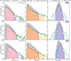 |
Fig. 1. Lyman-alpha luminosity (left panels), REW (middle panels), and UV absolute magnitude (MUV, right panels) distributions per unit volume for redshifts z = 2.4 (top panels), z = 3.1 (middle panels), and z = 4.5 (bottom panels). The solid green line shows the ODIN-COSMOS LAE sample (Lyα Lum ≥ 1042 erg s−1 and REW ≥ 20 Å), while the shaded gray area shows the same sample in the TNG100 simulation. The solid blue line shows a randomly selected subset representing 25%, 33%, and 40% of the LAEs in TNG100 at z = 2.4, 3.1, and 4.5, respectively. The shaded pink areas show the latter samples applying a minimum luminosity cut of 1042.04, 1042.18, and 1042.37 erg s−1 (vertical dashed line shown in the left panels), respectively. The shaded orange areas show the REW distributions noisified by photometric uncertainties, while the sky blue shaded regions show the corresponding noisified MUV distributions (see text). |
2.2. Mock data
We model LAEs following Andrews et al. (2025), who implement a model for LAE galaxies in The Next Generation Illustris (IllustrisTNG, Nelson et al. 2019; Pillepich et al. 2018). The IllustrisTNG is a set of magneto-hydrodynamical cosmological simulations run with the AREPO moving mesh code (Springel 2010). These simulations include sub-grid models that account for star formation, radiative metal-line gas cooling, chemical enrichment from supernovae types II and Ia, as well as asymptotic giant branch stars, stellar feedback, and supermassive black holes growth and kinetic feedback. The differing particle resolutions and box sizes render the IllustrisTNG simulations complementary, allowing them to be particularly useful for distinct analyzes depending on the specific goals of each study. In particular, IllustrisTNG100-1 (hereafter TNG100), is a box with a side length of 110.7 cMpc run using initial conditions with 18203 dark matter particles of mass 7.5 × 10⁶ M⊙ and 18203 gas cells with a mass of 1.4 × 10⁶ M⊙.
The LAE model follows the prescription given in Dijkstra & Wyithe (2012) and is further developed by Gronke et al. (2015), Weinberger et al. (2019). It assigns the Lyα luminosity, LLyα, to galaxies based on their UV luminosity density, LUV, ν, (in our case derived from Vogelsberger et al. 2020, model c), and a randomly drawn REW from a probability distribution function, P(REW | MUV), according to the following equation:
 (2)
(2)
where να = 2.47 × 10¹⁵ Hz, λα = 1216 Å, β = −1.7 is the UV spectral slope, and λUV = 1600 Ådenotes the rest-frame wavelength at which the UV continuum flux density was measured. The probability distribution P(REW | MUV) follows the form
 (3)
(3)
where REWc is a characteristic REW that depends on the UV magnitude, and N is a normalization constant. For more details, see Andrews et al. (2025).
In this work, we use the model applied to TNG100 with a lower stellar mass of M* > 108.14 M⊙ to ensure completeness of the modeled galaxy sample in TNG100. The resulting mock sample has the same minimum halo mass estimated from ODIN observations (Herrera et al. 2025), as well as similar clustering and bias obtained assuming a uniform HOD.
3. Samples of LAEs
3.1. LAE samples in IllustrisTNG
As with the ODIN data (Section 2.1), mock galaxies are classified as LAEs if they satisfy the same conditions, Lyα luminosity ≥1042 erg s−1 and REW ≥ 20 Å (gray shaded area in Fig. 1). However, we noticed that the number density of LAEs in TNG100 is higher than in ODIN-COSMOS, with values of (4 − 5)×10−3 Mpc−3 and 1 × 10⁻³ − 6 × 10⁻⁴ Mpc−3, respectively. This discrepancy between the observed and predicted number densities is expected as described by Andrews et al. (2025) and Dijkstra & Wyithe (2012) through a normalization factor F. The mismatch arises because the model does not fully capture the complexities of Lyα radiative transfer, including the internal structure and geometry of dust and gas, as well as the star formation histories of LAEs, which can add a stochastic component to LAE detection. Therefore, only a fraction of galaxies that satisfy the conditions to be detected as LAE actually make it into the observed LAE sample. This is likely due in part to viewing-angle effects, such as Lyα emission being unobscured only along certain lines of sight. Consequently, we randomly select a fraction of the simulated LAEs to match the observed amplitude of the distribution of ODIN LAE luminosities. For z = 2.4, we used 25% of the simulated sample, for z = 3.1, we used 33%, and for z = 4.5, we used 40%. These subsamples are shown as solid blue lines in Figure 1. It is important to note that this random subsampling alone does not guarantee that the space densities of the mock and observed samples will match. To achieve a precise correspondence, an additional criterion based on luminosity must be applied, as detailed below.
We also noticed an incompleteness in the observed Lyα luminosity distribution of ODIN-COSMOS LAEs compared to the mocks (see the left panels of Fig. 1), which can be attributed to limitations in the observational setup. This incompleteness is evident at the faint end of the distribution, where the number of LAEs is underestimated in the observational data. As a result, a clear drop in source counts is visible at lower luminosities. For that reason, we applied a minimum luminosity cut to the TNG100 LAEs to remove a percentage of the lowest-luminosity sources that are less complete in the observations. The cut was chosen to produce a volumetric number density that matches the number densities of the ODIN samples. This corresponds to luminosity thresholds of 1042.04 erg s−1 for z = 2.4, 1042.18 erg s−1 for z = 3.1 and 1042.37 erg s−1 for z = 4.5 (vertical dashed lines in the left panels of Fig. 1). These subsamples are shown in shaded pink histograms and are the TNG100 samples that we consider to identify the LAE multiples in later sections.
It is important to note that to make the mock catalogs comparable to the line-of-sight “thickness” of the observational data, we constructed 2D projections of the simulation over line-of-sight depths of ∼74 cMpc at z = 2.4, ∼60 cMpc at z = 3.1, and ∼50 cMpc at z = 4.5 (Lee et al. 2024). We added together different projection axes and several different random seeds when selecting the LAE fractions so as to match the comoving volumes of the observations at each redshift.
The left panels of Fig. 1 also show that ODIN-COSMOS LAEs exhibit a high-luminosity tail, which is typically attributed to the presence of AGNs (e.g., Konno et al. 2016; Sobral et al. 2018). This feature is not reproduced by the model as it does not include the AGN emission.
In addition, it is important to note that the model only reproduces systems with REWs up to 300 Å (middle panels of Fig. 1). Extremely high REW values (greater than 240 Å) observed in the ODIN-COSMOS sample may represent genuine signals (e.g., Inoue 2011; Kashikawa et al. 2012), but they could also result from spurious measurements introduced by low signal-to-noise ratios in photometry (Firestone et al. 2024). This discrepancy at the high end of the REW distribution appears to be a systematic effect introduced when real photometry is used. Specifically, the observed excess of high REW values could be driven by sources with large photometric uncertainties in the broadband filters used to estimate the continuum. These uncertainties would amplify the derived REWs, particularly for objects with faint continuum detections. To test this, we constructed a flat (top-hat) input REW distribution sampled from real ODIN data with associated photometric errors. By perturbing the narrowband and double broadband magnitudes within their 1σ uncertainties and recalculating the REW, we reproduce an artificial tail of high REW values. We find that this tail persists even when only the double broadband is noisified, which suggests that the broadband errors dominate the effect. This is consistent with expectations, as LAEs with large REWs are often faint in the continuum, leading to significant broadband uncertainties. To account for this in the mock sample, we applied a “noisification” procedure to the REW values derived from the model. The resulting mock sample, including these photometric uncertainties, is shown as the orange shaded distribution in Fig. 1. In this way, the tail of the high REWs is reproduced and no additional REW cut is required.
Regarding the UV magnitude distributions (right panels in Fig. 1), the observations display a greater dispersion toward both brighter and fainter values. At higher redshifts the ODIN-COSMOS distributions align well with those of the simulation samples once the stochastic fraction and the minimum LAE luminosity are adjusted for ODIN incompleteness. Once again, we aim to assess the effect introduced by using real broadband photometry in the continuum estimations. To do so, we compute the UV magnitudes from the noisified REW distributions, effectively assuming this noise is mostly due to the continuum flux estimate, using Equation (2). The resulting distributions are shown as sky blue shaded regions and exhibit increased scatter, which tends to better reproduce the observed MUV.
3.2. Analysis of LAE host halos in IllustrisTNG
Lyman-alpha emitting galaxies are crucial for understanding galaxy formation at high redshifts. However, their representativeness within the overall galaxy population remains uncertain. In TNG100, only 15%, 17%, and 18% of the total galaxy population are classified as LAEs at z = 2.4, z = 3.1, and z = 4.5, respectively, according to our LAE selection criteria (i.e., Lyα Lum ≥ the adopted threshold and REW ≥ 20 Å). These fractions suggest that LAEs may not fully represent the diversity of high-redshift galaxy populations. In Appendix B we further analyze the behavior of LAEs and their fraction relative to the total galaxy population, where we find that LAEs preferentially reside in halos of intermediate mass, as well as in galaxies with intermediate stellar masses and moderate star formation rates, consistently across the three redshifts.
Depending on the galaxy selection, more massive halos can host a greater number of galaxies. Here, we explore whether this is the case for the number of LAEs using a simulated catalog. Furthermore, we can make further tests, such as whether higher-mass halos contain more luminous LAEs, and whether the virial UV and Lyα luminosity densities depart from a constant value, as is the case of the virial mass density. Based on the analysis in Appendix B, we expect that only about 10 − 20% of massive halo populations are represented by LAEs. Therefore, we investigate whether multiple LAEs can be found within the same halo in our TNG100 samples. To do this, we examine the relationship between the halo mass M200 and the number of LAEs each halo contains.
The solid lines in Figure 2 show the mean mass of the modeled halos at the three redshifts as a function of the number of LAEs they contain. The LAE samples used here are defined in Section 3, based on the corresponding 2D projections. From this analysis, we find that ∼97 − 98% of LAEs are the only LAE within their host halo, which typically has a mean mass of M200 ∼ 1011.4 − 1011.9 M⊙, increasing toward lower redshifts. In other words, if we consider a survey that includes exclusively LAEs, we may safely assume that most of these galaxies are isolated. However, there are ∼2 − 3% of halos that host two LAEs, and about ∼0.1 − 0.2% that contain three or more. This is something we took into account to limit our selection of LAE multiples.
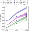 |
Fig. 2. Mean halo mass as a function of the number of LAEs within the halo at z = 2.4 (blue), z = 3.1 (magenta), and z = 4.5 (green). The TNG100 true multiples are shown with solid lines, while the TNG100 multiples identified using projected distances of rpmax = 100 pkpc at z = 2.4, 70 pkpc at z = 3.1 and 50 pkpc at z = 4.5 are displayed using dashed lines. Shaded regions and error bars show the error of the mean. As the number of LAEs in a halo increases, the true mean halo mass also increases, suggesting that the number of physically associated LAEs can serve as a proxy of halo mass. The identified multiples follow the underlying trend more closely at higher redshift. |
In addition, Figure 2 reveals that as the number of LAEs within a halo increases, the halo mass also increases. The mean M200 increases from 1011.9 to 1013 M⊙ at z = 2.4, from 1011.6 to 1012.5 M⊙ at z = 3.1, and from 1011.4 to 1012.26 M⊙ at z = 4.5 with increasing the number of LAEs from 1 to > 2.
Building on this, in the following Section we search for LAE multiples in the mock catalog and in ODIN. A mass dependence on LAE multiplicity implies that multiple LAEs are more likely to be influenced by interactions with nearby galaxies, potentially leading to observable differences in key physical properties such as stellar mass and star formation rate.
4. Identification of galaxy multiples
4.1. Optimizing the identification method
We now proceed to identify LAE multiples with the aim of identifying physically associated systems of varying masses and properties. To do so, we take advantage of the fact that our LAEs are located at similar redshifts due to the narrow width of the ODIN custom filters. The ODIN survey provides redshift precision of Δz ∼ 0.03 − 0.04, which is significantly better than the precision typically achievable with photometric redshifts derived from broadband filters (Δz ∼ 0.1 − 0.4 at z ≳ 2, e.g., Shi et al. 2020; Huang et al. 2022). Specifically, the FWHM of the N419, N501 and N673 filters corresponds to Δz = 0.061, 0.062 and 0.082, respectively, in redshift space (Lee et al. 2024).
Several methods for identifying galaxy systems have been developed over the years (e.g., Lambas et al. 2003; O’Mill et al. 2012). In this work, we adapt a technique originally applied to minor galaxy systems at low redshift (Cerdosino et al. 2024), modifying it for application to our high-redshift LAE samples. Robust system identification requires a methodology that carefully balances both the purity and completeness of detected systems. These two aspects are best evaluated using mock catalogs, which allow for precise control over the true physical associations between galaxies (e.g., Rodriguez et al. 2020). For this purpose, we use our mock LAE catalog (described in Section 3) which provides both the projected positions and host halo information for each LAE.
We computed the projected distances between LAEs and impose a minimum separation of 10 pkpc. This lower limit is motivated by the observational angular resolution of ODIN, which corresponds to ∼1.2, ∼1.3, and ∼1.5 arcsec at z = 2.4, z = 3.1, and z = 4.5, respectively. In cases where two mock LAEs are closer than this limit, we retain only the one with the higher Lyα luminosity. This minimum distance is consistent with definitions commonly adopted in other works on galaxy systems at high redshift (e.g., Matthee et al. 2023). While this choice represents a simplifying assumption, favoring the brighter source, in real observations such close pairs would be merged. Additionally, it is likely that not all the luminosity of the fainter unresolved source would be accounted for in the merged one. It is worth noting, however, that this situation accounts for fewer than 0.5% of galaxies in all cases. We also estimate that the impact of peculiar velocities is negligible, as they are on the order of a few hundred km s−1, representing only a small fraction of the survey depth.
To group the LAEs, we searched for neighboring LAEs within a maximum projected separation rpmax around each one and use a graph-based method to connect them. In this approach, pairs of galaxies separated by less than rpmax are linked without repeating galaxies, and the connected components of the resulting graph are interpreted as galaxy associations. Each association corresponds to a set of galaxies that are spatially connected to one another within the adopted distance threshold. We then determine the optimal value of rpmax that provides the best balance between contamination and completeness. We use two definitions to classify our LAE multiples. The first, “TNG100 true”, refers to cases where all LAEs are in the same halo in projection, without applying a maximum projected separation. The second, “TNG100 identified”, includes multiples identified in projection after imposing a maximum projected distance cut-off. This latter definition is intended to mimic the identification applied to observations.
To evaluate our selection method, we use two definitions: contamination and fraction of halos recovered (completeness). A detailed description of these definitions, together with the methodology used to compute them, is provided in Appendix A. To ensure that contamination remains reasonably low while maintaining a substantial fraction of recovered halos, we chose a maximum projected distance of 100 pkpc for z = 2.4, 70 pkpc for z = 3.1, and 50 pkpc for z = 4.5. This choice results in a recovered halo fraction of approximately 54%, 51%, and 54% with a contamination of about 55%, 58%, and 49% at z = 2.4, z = 3.1, and z = 4.5, respectively. These values were selected not only to balance completeness and contamination, but also to optimize the correlation between halo mass and the number of LAEs in the identified multiples (see next subsection).
These values of contamination are higher than what can be obtained with other low-z surveys (Cerdosino et al. 2024). Our current ODIN LAEs still contain limited information available only including UV luminosities, Lyα luminosities, and equivalent widths, with a fixed photometric redshift error. We carefully searched for ways to improve contamination using the true and falsely identified LAE associations in the TNG100 mocks and found no differences in the distributions of relative UV or Lyα luminosities that could have been used to help reduce contamination. As the survey progresses, the addition of physical properties estimated for the LAE candidates may help to improve future searches for multiples in ODIN. However, this first sample provides interesting insights into LAE groups and their physical properties, as we show below.
4.2. Multiples of LAEs
We used the TNG100 identified multiples to assess whether the median mass of the halos increases according to the number of associated LAEs, as previously observed for the TNG100 trues in Figure 2. The dashed blue line in that figure shows the multiples identified with a rpmax of 100 pkpc at z = 2.4, the dashed magenta line represents those identified with 70 pkpc at z = 3.1, and the dashed green line those with 50 pkpc at z = 4.5. The mean halo masses recovered from the TNG100-identified multiples follow the overall trend observed in the TNG100-true cases, with the correlation between halo mass and number of LAEs being more evident at higher redshifts. We observe a systematic effect that tends to lower the mean halo masses of identified groups with higher LAE multiplicity. This bias is primarily driven by the incorrect inclusion of low-mass, isolated LAEs in the identification of multiples, which artificially lowers the recovered masses.
Using the same rpmax values, we identified the multiples in the ODIN-COSMOS LAE sample. Table 1 presents the number of identified multiples for both the mock and observational datasets, as well as the percentage relative to the total number of LAEs in each sample.
Number and percentage of multiples.
The vast majority of LAEs in both the simulated and observational samples are isolated, with more than 96% of sources appearing as single LAEs across the three redshifts. Only a small fraction are identified as multiples of two LAEs (∼1 − 3%), and even fewer (≤0.2%) as part of larger associations. These trends are consistent across the TNG100-true, TNG100-identified, and ODIN-COSMOS samples. However, ODIN-COSMOS shows a slightly higher fraction of isolated LAEs (∼98 − 99%) and correspondingly lower percentage of higher-order multiples. The similarity between the TNG100 true and TNG100 identified multiplicity distributions suggests that our graph-based method is effective in retrieving the overall statistics of LAE multiples. The close agreement between the multiplicity statistics in the observational and TNG100 samples is strongly dependent on the stochasticity introduced when constructing the mock catalog, where only a fraction of the simulated LAEs is randomly selected. Without this selection step, the simulation produces a significantly larger number of LAE multiples, which is inconsistent with observational findings. This can be taken as an additional indication that the Lyα luminosity model applied to TNG100 galaxies is able to capture quite successfully the physics and stochasticity behind this type of emission. The small remaining discrepancy in the ODIN-COSMOS sample, particularly for associations with more than two members, may be attributed to observational limitations, such as ODIN sensitivity thresholds or projection effects due to the filter’s depth along the line of sight.
As discussed in Section 3 regarding the potential presence of AGNs in our sample of LAEs, we further classified our ODIN-COSMOS multiples into two categories: those in which all LAEs have Lyα luminosities less than 1043.5 erg s−1 and those containing at least one LAE with a Lyα luminosity exceeding this threshold, which could indicate the presence of a potential AGN (Konno et al. 2016; Sobral et al. 2018). The majority of the multiples are composed of LAEs with lower luminosities, with only ≤2% containing a possible AGN for the samples at redshifts 2.4 and 3.1. At z = 4.5, this percentage is a bit higher (3.4%). To compare these results with a matched random sample, we selected pairs and triples of isolated LAEs in higher proportions than those found in the identifications, choosing as many pairs and triples as possible from random realizations without replacement (27% for pairs and 18% for triples). The random sample yielded similar percentages: at z = 2.4 and z = 3.1, fewer than 2% of multiples have a LAE with luminosities above 1043.5 erg s−1, while slightly higher values (3 − 5%) are found at z = 4. Interestingly, none of the multiples consisting of more than 2 LAEs at z = 2.4 includes a potential AGN. However, this is similar to the result of the random samples indicating no clear relation between AGN activity and LAE multiplicity, an assertion that can be revisited with the larger final ODIN samples. Note that this behavior is not typically expected based on studies of protoclusters. At redshifts between 2 and 6, AGNs are often found to be more prevalent in overdense environments, as shown in several works (e.g., Lehmer et al. 2009; Casey et al. 2015; Shah et al. 2024). This contrasts with the local Universe, where AGN activity is generally suppressed in the densest regions, such as galaxy clusters, due to environmental quenching and gas stripping (e.g., Kauffmann et al. 2004). The enhanced AGN fraction at high redshift has been interpreted as evidence that black hole fueling is more efficient at earlier cosmic times, likely driven by processes such as mergers and interactions (e.g., Lemaux et al. 2022) but at least in our current sample we are not able to confirm this with ODIN.
5. Results
5.1. Dependency with Lyα luminosity and UV magnitude
To investigate the relationship between LAE multiplicity and intrinsic galaxy properties, we analyzed the mean Lyα luminosity and rest-frame UV magnitude of LAEs within identified multiples. In Figure 3, the top panels show the mean Lyα luminosity of individual LAEs as a function of the number of LAEs in multiples at the three redshifts: z = 2.4 (left), z = 3.1 (middle), and z = 4.5 (right). We compared the results for the TNG100-true (solid black lines), TNG100-identified (dashed pink lines), and ODIN-COSMOS (dotted cyan lines) datasets using the previously defined rpmax. To ensure a fair comparison, we considered only the ODIN-COSMOS multiples with Lyα luminosities below 1043.5 erg s−1, thus avoiding possible AGN contaminants.
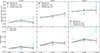 |
Fig. 3. Mean Lyα luminosity (top panels) and UV magnitude (bottom panels) as a function of the LAE multiplicity for redshifts z = 2.4 (left), z = 3.1 (middle), and z = 4.5 (right). Solid black lines correspond to the TNG100-true multiples, dashed pink lines show the TNG-identified multiples (with rpmax = 100 pkpc at z = 2.4, 70 pkpc at z = 3.1, and 50 pkpc at z = 4.5), and dotted cyan lines correspond to the ODIN-COSMOS sample under the same selection criteria. The lighter black and pink lines indicate the mean UV magnitudes perturbed by photometric uncertainties for the mock samples. Error bars represent the standard error of the mean. Overall, both Lyα luminosity and UV magnitude tend to increase slightly with LAE multiplicity, supporting the idea that multiple LAEs trace more massive and actively star-forming halos. |
We find that the mean Lyα luminosity either shows a slight tendency to increase with multiplicity or remains roughly constant in the mock samples (except for the TNG100 true sample at z = 2.4, where it decreases for multiples with more than two LAEs). In the observational data, this trend is more evident at z = 2.4 and z = 4.5, suggesting that higher multiplicity systems at these redshifts are preferentially associated with more luminous LAEs, assuming the incompleteness and contamination are similar to those in the mock. We also performed a comparison with a random sample of pairs and triples drawn from the isolated LAEs, finding that their mean luminosities and magnitudes remain constant. This supports the interpretation that the observed variations in the real sample reflect a genuine trend. However, it should be noted that the dispersion introduced by the error bars prevents us from establishing a conclusive trend, particularly for the TNG100-true sample at z = 2.4 which shows an opposite behavior. Furthermore, the offset between the mock and ODIN-COSMOS mean values could reflect the effects of contamination and incompleteness in the identification process, as discussed earlier.
Both the halo mass (Fig. 2) and the mean Lyα luminosity show an increase with redshift. This result, however, seems to be at odds with Khostovan et al. (2019) and Herrero Alonso et al. (2023) who find no significant redshift evolution in the typical halo masses hosting LAEs, indicating that LAEs reside in halos of similar mass across cosmic time. Moreover, Herrero Alonso et al. (2023) points to the possibility that the observed clustering dependence on Lyα luminosity is driven by cosmic evolution of the clustering of objects of similar mass.
The bottom panels of Fig. 3 display the mean MUV magnitudes as a function of LAE multiplicity. A similar trend is observed in the mock samples: LAEs show a weak tendency to be more UV-luminous as the multiplicity increases. This indicates that more massive halos hosting higher LAE multiplicities could also drive more vigorous star formation. However, the ODIN-COSMOS sample shows a significant dependence on the LAEs of multiples with more than 2 LAEs. We also show, in gray and lighter pink, the mean noisyfied MUV magnitudes (as described in Section 3) for the TNG100-true and TNG100-identified samples, and they follow similar trends as the noise-free magnitudes.
Our samples of multiple LAEs appear to exhibit broadly consistent trends between the mock and observational data, with a possible increase in the mean Lyα and UV luminosities as the number of LAEs per multiple rises. These multiples represent physical associations of star-forming galaxies at relatively high redshifts, where star formation is at its densest in the history of the Universe. We therefore attempt to characterize the local conditions where these LAEs reside in the following subsection, and in the subsequent one, we propose a method to test the physical connection between LAE multiples and star formation due to the presence of perturbing neighbors.
5.2. Group-wide Lyα and UV luminosity surface densities
In this section, we analyze the virial projected Lyα and UV luminosity densities of LAEs, defined as the sum of the luminosities of all galaxies in a multiple, divided by an estimate of the projected area of the halo. These quantities can help to gain insights into the star formation processes within virialized halos and their relation to the presence of physically associated neighbors. By examining the correlation between the local UV luminosity virial density, and observable quantities, such as the number of LAEs or the relative fraction of LAEs among halo galaxies (accessible in simulations), we hope to obtain insights into how star formation activity is distributed within halos and whether the presence of LAEs in multiples affects this distribution.
We define the virial luminosity density, corresponding to the total Lyα (or UV) luminosity of LAEs or galaxies, as the sum of their individual luminosities divided by the projected area π ⋅ (distmax/2)2 computed using two distinct but closely related spatial scales in the simulations and the one available to ODIN for observations. The “physical scale” corresponds to the maximum 3D radius that contains all galaxies within a given halo. We defined distmax as the largest 3D separation between any two halo member galaxies. This scale provides a comprehensive view of the luminosity distributions across the full extent of the halos in the mock and are presented in the left panels of Figure 4. The “observational scale” was defined observationally (in the mock and in ODIN), where distmax represents the maximum projected radius that encloses the galaxies identified as part of a LAE multiple. This approach uses observationally available information and aligns directly with ODIN data, where only LAEs are mapped, ensuring consistency in system-size measurements. For high multiplicities, distmax is defined as the maximum projected separation between all LAEs, corrected by a factor in the case of pairs to account for central–satellite and satellite–satellite configurations which we obtained from the mock catalog. For isolated LAEs, distmax was set as the mean projected separation of the two-LAE multiples. This observational-scale analysis is shown in the right panels of Fig. 4.
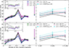 |
Fig. 4. Virial surface brightness of Lyα (erg s−1 kpc−2) and UV (erg s−1 Hz−1 kpc−2) luminosities as a function of LAE multiplicity. Left panels: Mean virial surface luminosities for Lyα (top) and UV (bottom) emissions in TNG100, defined as the total luminosity per projected area, at z = 2.4 (blue), z = 3.1 (magenta), and z = 4.5 (green), plotted as a function of the fraction of LAEs relative to the total number of galaxies in the halo. Solid lines correspond to LAE-based densities, while dotted lines correspond to galaxy-based densities. Insets display the mean total luminosity before normalization. Error bars represent the standard error of the mean. Both Lyα and UV virial densities increase with the LAE fraction, reaching a peak at ∼0.5. This behavior is mainly driven by the Lyα model, which produces a more compact spatial distribution of LAE galaxies within halos. Right panels: Mean virial surface luminosities as a function of LAE multiplicity. Black lines show the TNG100-true values, pink lines show the TNG100-identified sample, and cyan lines are for the ODIN-COSMOS data. The solid, dashed, and dotted line styles denote z = 2.4, z = 3.1, and z = 4.5, respectively. Error bars represent the standard error of the mean in each bin. Higher LAE multiplicity appears to be associated with increased virial surface brightness densities. |
The left panels of Fig. 4 show the mean total Lyα luminosity (top panel) and UV luminosity (bottom) of normal galaxies (dotted lines) and LAEs (solid lines) in the mock catalog at z = 2.4 (blue), z = 3.1 (magenta) and z = 4.5 (green), normalized by the physical-scale area, as a function of the number of LAEs relative to the total number of galaxies in the halo. At high LAE fractions (> 0.4), the densities traced by all galaxies closely follow that traced by LAEs, indicating that halos with high LAE fractions are predominantly UV- or Lyα-luminous due to LAEs themselves. At lower fractions, a divergence emerges, especially in the case of UV, reflecting contributions from non-LAE galaxies. The agreement is tighter in Lyα across the entire LAE fraction range.
For LAEs, both Lyα and UV densities increase with increasing LAE fraction, peaking at around ∼0.5, although errorbars for this fraction are large as this point receives contributions from halos with pairs or a few LAEs. Errors diminish for larger fractions which correspond to halos with larger numbers of LAEs. This behavior suggests that the adopted Lyα luminosity model predicts a higher fraction of LAEs in regions with enhanced UV radiation density from star formation – at least up to halos with LAEs making up half the halo population. Notably, this trend is not driven by changes in the average UV or Lyα luminosity of LAEs and normal galaxies. As shown in the insets, the mean total Lyα luminosity remains approximately constant, while the UV luminosity slightly decreases with increasing LAE fraction. This highlights that the increase in surface densities arises primarily from the Lyα model tending to produce a more compact spatial distribution of LAE galaxies, rather than from intrinsic luminosity enhancements.
For our previously defined sample of LAE multiples, the right-hand panels of Fig. 4 show the mean total Lyα luminosity (top) and UV luminosity (bottom) of LAEs within each multiple, normalized by the observational-scale area, as a function of LAE multiplicity at z = 2.4 (solid lines), z = 3.1 (dashed lines) and z = 4.5 (dotted lines). In both cases, the virial surface density values are systematically higher at z = 4.5 than at z = 3.1, which in turn are higher than at z = 2.4, suggesting more intense star formation activity or more compact associations at earlier cosmic times for both ODIN-COSMOS and TNG100 multiples.
Both the TNG100-identified sample and the ODIN-COSMOS data also exhibit a positive trend, with higher LAE multiplicity associated with increased virial surface brightness densities. This supports the hypothesis that environments hosting multiple LAEs are more actively star-forming and/or denser, which enhances both Lyα and UV emission densities. However, the TNG100-true sample shows a different behavior, particularly at z = 2.4. In this case, the projected separations (rpmax) of true systems can reach up to ∼700 pkpc. Due to our imposed rpmax cut for multiples identification, many of these extended multiples are split into multiple smaller multiples or identified as isolated LAEs, underestimating the true multiplicity. As a result, the surface brightness appears to decline at high multiplicities. At z = 3.1 and 4.5, halos are generally more compact, and this issue is mitigated, leading to a more consistent trend with increasing multiplicity. Still, the increase in luminosity density of identified multiples could be an artifact of the identification rather than a physical trend.
It is important to note that this trend could be affected by the method adopted to define the radius of the virialized object. However, we find that it is also present when the normalization is defined using the average value of the halo radius, R200 (see Fig. C.1 in Appendix C) corresponding to each sample.
It should still be noticed the excellent consistency between the mock and ODIN observations, which supports the validity of the Lyα emission model by Dijkstra & Wyithe (2012) in accurately reproducing the observed properties of LAE multiples within dark matter halos (with our samples). This agreement suggests that the model effectively captures the key physical processes governing Lyα radiative transfer and star formation activity in dense environments, such as those traced by multiple LAEs in the same halo.
With larger samples such as the full ODIN survey, it may be possible to have a better sample of multiples with many LAEs. Confirming an increasing or decreasing trend of virial UV and Lyα luminosity density in multiples, unaffected by the low number statistics and the fragmentation of halos into pairs or triplets, could help put star formation in the framework of disk instabilities set off by perturbers.
The insights of Mo et al. (1998), which point that bursts of star formation can take place in flattened gas disks because they are susceptible to perturbations that can ignite star formation and consume the gas within them, could be put to the test with the full ODIN survey, given the expected high star formation activity of LAEs. In a halo containing multiple galaxies (subhalos), it is plausible that interactions among these galaxies act as the triggers for such perturbations, leading to significant hydrogen line emissions, as is characteristic of Lyα emitting galaxies. Alternatively, the triggering of star formation could also be due to direct infall of cold gas, as proposed by Dekel et al. (2009). We next make an attempt to tell these two possible effects apart with the mock catalog.
5.3. Star formation due to instabilities triggered by members of LAE multiples
We tested whether star formation in LAEs is driven by nearby perturbations using the mock LAE samples extracted from TNG100. This analysis is further motivated by the apparent excess of disk morphologies seen in galaxies at the ODIN-COSMOS redshifts, as revealed from optical rest-frame imaging by JWST (e.g., Kuhn et al. 2024). It is important to note that the degree of star formation enhancement resulting from such perturbations may vary across different simulations, depending on the specific numerical implementations of the star formation models. While perturbations can generally induce local density peaks that may promote star formation, the extent of this enhancement is sensitive to the adopted subgrid physics and feedback prescriptions.
We started by assuming that all galaxies within the halo experience a perturbation capable of triggering a star-forming event when the perturber induces a change in the disk gravitational potential proportional to the disk’s own gravitational potential by a factor fϕ:
 (4)
(4)
Here, Δϕ and ϕd are the perturbation and disk gravitational potentials, respectively, and we write the disk potential as a function of its mass (Md) and radius (Rd).
Assuming that subhalos have a minimum mass (Msh, min) and taking advantage of the steep slope of the subhalo mass function, we adopted the approximation that only subhalos with this minimum mass are present in the halo. Under this assumption, the perturbation can be approximated by the gravitational potential of these subhalos,
 (5)
(5)
where ⟨dsh, min⟩ is the mean distance between substructures. Combining Eqs. (4) and (5), we found
 (6)
(6)
Considering that Vsh, min, a cubic volume with side length of ⟨dsh, min⟩, and that the mass (or volume) of the halo can be approximated as the product of the number of subhalos and their respective masses (or volumes), we can express
 (7)
(7)
where ρc(z) is the critical density at that redshift. For our calculations, we assumed that the mass and radius of the disk are proportional to the mass and radius of the subhalo following the relations Md = fMMsh and Rd = fRRsh, where Msh is the total mass for the subhalo and Rsh is the subhalo half mass radius. Consequently, Equation (7) depends on the perturbation factor fϕ and the ratio of the proportionality factors fM/fR. This ratio fM/fR reflects the relationship between the fraction of the subhalo mass contributing to the galaxy’s disk (fM) and the fraction of the subhalo’s radius defining the galaxy’s disk size (fR). This parameter essentially encapsulates how the properties of the subhalo translate into the disk characteristics, such as its gravitational potential and physical extent. This approach allows us to explore the relationship between subhalo interactions and, in our particular case, LAEs.
Using the values of Msh and Rsh for the galaxies from TNG100, together with Md and Rd from the literature, we can obtain a simple estimate of the ratio fM/fR. For this, we adopt the results of Ma et al. (2024), who measured the cold gas mass and half-mass radius for different galaxy samples at different redshifts in TNG50. For consistency with our analysis, we use their most massive sample (referred to in their paper as M4), which matches the properties of the LAEs in TNG100. We obtain the mean values of fM/fR = 2.43, 0.78, and 0.63 at redshifts 2.4, 3.1, and 4.5, respectively. Using these values and varying the perturbation factor fϕ, we can test how well our model reproduces the distribution of subhalo masses and gain insight into the role of subhalos in driving galaxy evolution.
Figure 5 presents the resulting distributions of the minimum subhalo masses obtained using our model with TNG100 and its various subsets, at z = 2.4 (left panels), z = 3.1 (middle panels), and z = 4.5 (right panels). For comparison, the top panels display the distribution of minimum subhalo masses for all TNG100 halos as shaded black histograms. The model predictions for the full galaxy sample are shown as dashed black lines, using the fM/fr values mentioned above and the fϕ values that minimize the difference between the expected and model histograms. We find fϕ = 0.11, 0.39, and 0.50 at z = 2.4, 3.1, and 4.5, respectively. The model generally shows good agreement with the actual masses of subhalos in the simulation, but tends to underpredict the low-mass tail, which is largely introduced by satellite galaxies that the model fails to reproduce. In addition, it overpredicts the number of high-mass central subhalos, leading to an artificial excess at the high-mass end. The perturbation factor fϕ increases with redshift, indicating that stronger perturbations are required to trigger star formation at earlier cosmic times. Note that it is quite unlikely that a perturber will induce fϕ > 0.1 as this would imply strong interactions. We interpret the values for this quantity obtained for z = 3.1 and 4.5 as indications that, at least in the simulation, the instabilities driving star formation are not due to interactions with other satellites (in line with Dekel et al. 2009). Colored shaded histograms show the minimum subhalo masses for halos hosting LAEs, while the colored dashed lines represent the model predictions for all TNG100 LAEs using the same scaling factors. In this case, the fit improves significantly, as LAEs do not exhibit the low- or high-mass tails seen in the full halo sample. In the middle and bottom panels, we compare the minimum masses of the LAE subhalos with the model applied to the TNG100 True multiples with one (dotted orange lines, middle panels) and two (dash-dotted red lines, bottom panels) LAEs, with the same parameters.
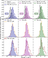 |
Fig. 5. Distribution of minimum subhalo masses in the halos at z = 2.4 (left panel), z = 3.1 (middle panel), and 4.5 (right panel). In the top panels, the minimum subhalo mass distributions from TNG100 are shown as shaded black histograms, while the model predictions described in Section 5.3 are overplotted as dashed black lines (with fϕ = 0.11 and fM/fr = 2.43 at z = 2.4, fϕ = 0.39 and fM/fr = 0.78 at z = 3.1, and fϕ = 0.50 and fM/fr = 0.63 at z = 4.5). Using these factors, we test the model against all TNG100 LAEs (colored dashed lines in the top panels), TNG100 true 1 LAEs (dotted orange lines in the middle panels), and TNG100 true 2 LAEs (dash-dotted red lines in the bottom panels), comparing them with the corresponding minimum subhalo mass distributions of TNG100 LAES (shaded colored histograms). The model shows a good agreement with the minimum subhalo mass distribution for all galaxies, for all LAEs, and isolated LAEs, but struggles to reproduce as closely the distribution for LAE pairs. |
It is significant that the model successfully reproduces the distribution of the minimum subhalo mass present in the simulation at z = 2.4 with a reasonable level required for the perturbation of the potential. This alignment suggests that indeed the simulation effectively traces subhalo-driven perturbations at z ≲ 3, which are critical for triggering star formation. Such consistency is expected, as the star formation prescription in IllustrisTNG includes the requirement that the gas forming stars must be in a locally collapsing state. This condition naturally aligns with the onset of instabilities, which can be induced by intra halo perturbations among other processes such as cold gas inflows. Therefore, the ability to match Msh, min in the mock at these lower redshifts lends confidence to both the simulation’s physical modeling and our interpretation of a shift from subhalo driven to cold flows perturbations at z > 3 a crucial test that will hopefully be achievable with the full ODIN survey.
It is interesting to note that the inferred fϕ perturbation factor can be used to fit the underlying minimum subhalo mass distribution for all galaxies, LAEs, and LAEs in single multiples. The agreement between single LAEs – not necessarily isolated as they can have non-LAE satellites – and the overall LAE distribution is largely reproduced, as isolated LAEs constitute the majority of the sample. In contrast, applying the same model values to pairs of LAEs yields multimodal distribution but still in reasonable agreement, with the slight discrepancies showing signs of an increase at higher redshifts. This result again suggests that the presence of a neighboring LAE influences star formation activity at z = 2.4, at least within the framework of this model.
The minimum mass threshold which is reproduced by our model with a reasonable level of perturbation of the potential for z = 2.4 also hinges on the fraction of LAEs that we select in order to reproduce the abundance of observed LAEs. In future work one can improve the model also taking into account the expected recurrence timescale of such events. In halos hosting multiple subhalos above Msh, min, the typical orbital periods of these companions could naturally lead to quasi-periodic episodes of enhanced star formation and Lyα emission that would explain the fraction that we apply by hand. In this framework, the observed multiplicity of LAEs and their visible fraction could be seen as a tracer of the characteristic duty cycle of their Lyα-bright phases.
6. Conclusions
In this study, we used data from the ODIN survey–the largest narrowband filter survey conducted to date. The survey employs three custom-designed narrowband filters to detect LAEs across three equally spaced epochs in cosmic history. Using the LAE samples at redshifts 2.4, 3.1, and 4.5, we searched for multiple LAE associations as a proxy for halo masses. This approach was supported by an analysis using a model (Dijkstra & Wyithe 2012) that reproduces the LAE population, and it was applied to the IllustrisTNG100 simulations (Andrews et al. 2025). These simulations allowed us to test our selection method and test for systematic effects present in the comparison. To this end, we constructed a sample of LAEs that is consistent between simulations and ODIN observations. Our main results are listed below.
-
In the mock catalog, we find that it is possible to find physical multiples of LAEs, with controlled contaminants and reasonable completeness. The resulting multiples show a clear correlation between the number of LAEs and the mass of their host dark matter halos. Although most LAEs are isolated, systems with a higher multiplicity tend to reside in more massive halos. Our method for selecting LAE multiples successfully recovers this trend to a significant degree.
-
In both ODIN and mock samples, we find indications that the mean Lyα luminosity and UV magnitudes of LAEs in the multiples increase with multiplicity, supporting a connection between Lyα emission, multiplicity, and halo mass. However, this trend is not conclusive given the dispersion of the error bars, and further statistical analysis is required to confirm or refute it.
-
The UV and Lyα virial (or halo-wide) surface brightness densities increase with LAE multiplicity, suggesting that more massive halos trace denser, more actively star-forming regions. Tests with the mock catalog suggest that this trend seems to be driven by a spatial compactness of LAEs and not by higher individual luminosities. We also find that LAEs are able to trace the UV virial density in an unbiased way. We observed a redshift dependence, with higher halo-wide surface brightness densities at z = 4.5 and z = 3.1 than at z = 2.4, consistent with more vigorously star-forming environments at earlier cosmic times.
-
We find strong agreement between the modeled and ODIN-COSMOS fractions of singles and higher-membership multiples. This trend is also consistent with the observed Lyα properties. These results validate the Lyα emission model by Dijkstra & Wyithe (2012) and Andrews et al. (2025), confirming its ability to reproduce the spatial and radiative characteristics of LAEs within dark matter halos.
-
Our subhalo-based model for perturbation-triggered star formation events accurately reproduces the minimum subhalo mass distribution of TNG100 LAEs for the z = 2.4 sample, supporting the idea that intra-halo perturbations–rather than LAE companions–are key to triggering star formation in these galaxies. Interestingly, at higher redshifts, we find that the required level of perturbation suggests that in TNG100, star formation is likely triggered by processes other than gravitational perturbations by subhalos.
Ultimately, our findings from the ODIN survey, corroborated by IllustrisTNG100 simulations, robustly establish Lyα emitter multiplicity as a powerful and observationally accessible proxy for tracing dark matter halo masses and the underlying processes of star formation in the distant Universe, thereby significantly advancing our understanding of galaxy evolution in cosmic dawn environments. The full ODIN survey will not only provide a larger sample of LAEs but also a wide set of physical properties derived from spectral energy distribution fitting, such as stellar mass and age, as well as structural parameters, such as galaxy size and morphology, from Hubble Space Telescope or JWST imaging. The availability of these ODIN LAE data will enable future analyses of correlations with additional physical properties.
Acknowledgments
This work utilizes observations at Cerro Tololo InterAmerican Observatory, NSF’s NOIRLab (Prop. ID 2020B0201; PI: K.S.L.), which is managed by the Association of Universities for Research in Astronomy under a cooperative agreement with the National Science Foundation. This work has been partially supported with grants from Agencia Nacional de Promoción Científica y Tecnológica, the Consejo Nacional de Investigaciones Científicas y Técnicas (CONICET, Argentina) and the Secretaría de Ciencia y Tecnología de la Universidad Nacional de Córdoba (SeCyT-UNC, Argentina). MCC acknowledges support from a CONICET Doctoral Fellowship. NP acknowledges support from PICT 2021-0700 and PICT Raices Federal 2023-0002. This material is based upon work supported by the NSF Graduate Research Fellowship Program under Grant No. DGE-2233066 to NF. EG and NF acknowledge support from NSF grant AST-2206222 and DOE grant DE-SC0010008. KSL acknowledges financial support from the National Science Foundation under grant Nos. AST-2206705 and AST-2408359, and from the Ross-Lynn Purdue Research Foundations. CG acknowledges support from NSF AST-240538. LG also gratefully acknowledges financial support from ANID – MILENIO – NCN2024_112, from FONDECYT regular project number 1230591, and from the ANID BASAL project FB210003. HSH acknowledges the support of Samsung Electronic Co., Ltd. (Project Number IO220811-01945-01), the National Research Foundation of Korea (NRF) grant funded by the Korea government (MSIT), NRF-2021R1A2C1094577, and Hyunsong Educational & Cultural Foundation. SL acknowledges support from the National Research Foundation of Korea (NRF) grant (RS-2025-00573214) funded by the Korea government (MSIT).
References
- Aihara, H., AlSayyad, Y., Ando, M., et al. 2019, PASJ, 71, 114 [Google Scholar]
- Andrews, M., Artale, M. C., Kumar, A., et al. 2025, A&A, 698, A280 [NASA ADS] [CrossRef] [EDP Sciences] [Google Scholar]
- Behroozi, P. S., Wechsler, R. H., & Conroy, C. 2013, ApJ, 770, 57 [NASA ADS] [CrossRef] [Google Scholar]
- Berlind, A. A., & Weinberg, D. H. 2002, ApJ, 575, 587 [Google Scholar]
- Casey, C. M., Cooray, A., Capak, P., et al. 2015, ApJ, 808, L33 [NASA ADS] [CrossRef] [Google Scholar]
- Cerdosino, M. C., O’Mill, A. L., Rodriguez, F., et al. 2024, MNRAS, 528, 4993 [Google Scholar]
- Dekel, A., Birnboim, Y., Engel, G., et al. 2009, Nature, 457, 451 [Google Scholar]
- Dijkstra, M. 2014, PASA, 31, e040 [Google Scholar]
- Dijkstra, M., & Wyithe, J. S. B. 2012, MNRAS, 419, 3181 [NASA ADS] [CrossRef] [Google Scholar]
- Firestone, N. M., Gawiser, E., Ramakrishnan, V., et al. 2024, ApJ, 974, 217 [Google Scholar]
- Firestone, N. M., Gawiser, E., Iyer, K. G., et al. 2025, ApJ, 986, L8 [Google Scholar]
- Flaugher, B., Diehl, H. T., Honscheid, K., et al. 2015, AJ, 150, 150 [Google Scholar]
- Gawiser, E., Francke, H., Lai, K., et al. 2007, ApJ, 671, 278 [NASA ADS] [CrossRef] [Google Scholar]
- Gronke, M., Dijkstra, M., Trenti, M., & Wyithe, S. 2015, MNRAS, 449, 1284 [Google Scholar]
- Guaita, L., Gawiser, E., Padilla, N., et al. 2010, ApJ, 714, 255 [NASA ADS] [CrossRef] [Google Scholar]
- Herrera, D., Gawiser, E., Benda, B., et al. 2025, ApJ, 988, L57 [Google Scholar]
- Herrero Alonso, Y., Miyaji, T., Wisotzki, L., et al. 2023, A&A, 671, A5 [NASA ADS] [CrossRef] [EDP Sciences] [Google Scholar]
- Huang, Y., Lee, K.-S., Cucciati, O., et al. 2022, ApJ, 941, 134 [Google Scholar]
- Im, S. H., Hwang, H. S., Park, J., et al. 2024, ApJ, 972, 196 [Google Scholar]
- Inoue, A. K. 2011, MNRAS, 415, 2920 [NASA ADS] [CrossRef] [Google Scholar]
- Jun, R. L., Theuns, T., Moriwaki, K., & Bose, S. 2025, MNRAS, 543, 1494 [Google Scholar]
- Kashikawa, N., Nagao, T., Toshikawa, J., et al. 2012, ApJ, 761, 85 [NASA ADS] [CrossRef] [Google Scholar]
- Kauffmann, G., White, S. D. M., Heckman, T. M., et al. 2004, MNRAS, 353, 713 [Google Scholar]
- Kawanomoto, S., Uraguchi, F., Komiyama, Y., et al. 2018, PASJ, 70, 66 [Google Scholar]
- Khostovan, A. A., Sobral, D., Mobasher, B., et al. 2019, MNRAS, 489, 555 [Google Scholar]
- Konno, A., Ouchi, M., Nakajima, K., et al. 2016, ApJ, 823, 20 [Google Scholar]
- Kuhn, V., Guo, Y., Martin, A., et al. 2024, ApJ, 968, L15 [NASA ADS] [CrossRef] [Google Scholar]
- Kumar, A., Artale, M. C., Montero-Dorta, A. D., et al. 2025, A&A, 698, A236 [NASA ADS] [CrossRef] [EDP Sciences] [Google Scholar]
- Kunth, D., Mas-Hesse, J. M., Terlevich, E., et al. 1998, A&A, 334, 11 [NASA ADS] [Google Scholar]
- Kusakabe, H., Shimasaku, K., Ouchi, M., et al. 2018, PASJ, 70, 4 [Google Scholar]
- Lai, K., Huang, J.-S., Fazio, G., et al. 2008, ApJ, 674, 70 [Google Scholar]
- Lambas, D. G., Tissera, P. B., Alonso, M. S., & Coldwell, G. 2003, MNRAS, 346, 1189 [NASA ADS] [CrossRef] [Google Scholar]
- Lee, K.-S., Gawiser, E., Park, C., et al. 2024, ApJ, 962, 36 [Google Scholar]
- Lehmer, B. D., Alexander, D. M., Geach, J. E., et al. 2009, ApJ, 691, 687 [Google Scholar]
- Lemaux, B. C., Cucciati, O., Le Fèvre, O., et al. 2022, A&A, 662, A33 [NASA ADS] [CrossRef] [EDP Sciences] [Google Scholar]
- Ma, H.-C., Du, M., Ho, L. C., Sheng, M.-J., & Liao, S. 2024, A&A, 689, A293 [NASA ADS] [CrossRef] [EDP Sciences] [Google Scholar]
- Matthee, J., Sobral, D., Oteo, I., et al. 2016, MNRAS, 458, 449 [Google Scholar]
- Matthee, J., Mackenzie, R., Simcoe, R. A., et al. 2023, ApJ, 950, 67 [NASA ADS] [CrossRef] [Google Scholar]
- Mo, H. J., Mao, S., & White, S. D. M. 1998, MNRAS, 295, 319 [Google Scholar]
- Nelson, D., Springel, V., Pillepich, A., et al. 2019, Comput. Astrophys. Cosmol., 6, 2 [Google Scholar]
- Okamoto, T., Gao, L., & Theuns, T. 2008, MNRAS, 390, 920 [Google Scholar]
- O’Mill, A. L., Duplancic, F., García Lambas, D., Valotto, C., & Sodré, L. 2012, MNRAS, 421, 1897 [CrossRef] [Google Scholar]
- Ono, Y., Ouchi, M., Shimasaku, K., et al. 2010, ApJ, 724, 1524 [NASA ADS] [CrossRef] [Google Scholar]
- Ouchi, M., Shimasaku, K., Furusawa, H., et al. 2003, ApJ, 582, 60 [Google Scholar]
- Ouchi, M., Ono, Y., & Shibuya, T. 2020, ARA&A, 58, 617 [Google Scholar]
- Partridge, R. B., & Peebles, P. J. E. 1967, ApJ, 147, 868 [Google Scholar]
- Pillepich, A., Springel, V., Nelson, D., et al. 2018, MNRAS, 473, 4077 [Google Scholar]
- Planck Collaboration XIII. 2016, A&A, 594, A13 [NASA ADS] [CrossRef] [EDP Sciences] [Google Scholar]
- Ramakrishnan, V., Lee, K.-S., Firestone, N., et al. 2025, ApJ, 982, 74 [Google Scholar]
- Rodriguez, F., Gonzalez, E. J., O’Mill, A. L., et al. 2020, A&A, 634, A123 [NASA ADS] [CrossRef] [EDP Sciences] [Google Scholar]
- Shah, E. A., Lemaux, B. C., Forrest, B., et al. 2024, ArXiv e-prints [arXiv:2409.02996] [Google Scholar]
- Shi, K., Toshikawa, J., Cai, Z., Lee, K.-S., & Fang, T. 2020, ApJ, 899, 79 [Google Scholar]
- Sobral, D., Matthee, J., Darvish, B., et al. 2018, MNRAS, 477, 2817 [Google Scholar]
- Springel, V. 2010, MNRAS, 401, 791 [Google Scholar]
- Venemans, B. P., Röttgering, H. J. A., Miley, G. K., et al. 2005, A&A, 431, 793 [NASA ADS] [CrossRef] [EDP Sciences] [Google Scholar]
- Vogelsberger, M., Nelson, D., Pillepich, A., et al. 2020, MNRAS, 492, 5167 [NASA ADS] [CrossRef] [Google Scholar]
- Weinberger, L. H., Haehnelt, M. G., & Kulkarni, G. 2019, MNRAS, 485, 1350 [NASA ADS] [CrossRef] [Google Scholar]
- Yang, X., Mo, H. J., & van den Bosch, F. C. 2008, ApJ, 676, 248 [Google Scholar]
- Zehavi, I., Contreras, S., Padilla, N., et al. 2018, ApJ, 853, 84 [NASA ADS] [CrossRef] [Google Scholar]
Appendix A: Contamination and completeness of LAE multiples
This Appendix presents the definitions and methodologies used to quantify contamination and completeness, which are applied in Section 4 to test our selection method for LAE multiples.
We define contamination as the fraction of detections in which not all members belong to the same halo (i.e., incorrectly identified associations), relative to the total number of true multiples. The left panel of Figure A.1 shows the contamination at the three redshifts (z = 2.4 in blue, z = 3.1 in magenta, and 4.5 in green). The solid lines represent all recovered multiples, while the dashed and dotted lines show the fractions corresponding to associations with 2 and 3 LAEs, respectively. As associations with 2 LAEs constitute the majority, the dashed line closely follows the total. We observe that contamination grows dramatically with projected distance, as expected due to the depth of the data, with only the smallest projections ensuring that the contamination is not unreasonably high. This analysis also reveals that multiples with more LAEs exhibit lower contamination, indicating they are more reliable tracers and more likely to reside within the same halos. However, such multiples are relatively rare in the present ODIN sample we analyze here.
On the other hand, we define the completeness as the fraction of recovered halos (with at least two galaxies). This is shown in the right panel of Figure A.1 as a function of the maximum projected distance (solid lines). As expected, this fraction increases with projected distance.
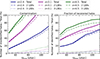 |
Fig. A.1. Fraction of detections in which not all members belong to the same halo (contamination, left panel) and fraction of halos with at least two galaxies that are recovered (completeness, right panel), as a function of the maximum projected distance rpmax, for the mock samples at z = 2.4 (blue), z = 3.1 (magenta) and z = 4.5 (green). The total fractions are shown with solid lines, while the fractions corresponding multiples of 2 LAEs are shown with dashed lines, and multiples of 3 LAEs with dotted lines. Both the contamination and the fraction of recovered halos increases with the rpmax, so it is necessary to find a compromise value between them. |
Appendix B: Analysis of LAEs (central and satellite) in IllustrisTNG
LAEs may not fully capture the diversity of high-redshift galaxy populations. In TNG100, only 15%, 17%, and 18% of galaxies are classified as LAEs at z = 2.4, z = 3.1, and z = 4.5, respectively, according to our LAE criteria (i.e., Lyα luminosity above the adopted threshold and REW ≥ 20 Å). Here, we analyze the fractions of LAEs relative to the overall galaxy population within halos and investigate how these fractions vary with different halo and galaxy properties.
The upper panel of Figure B.1 illustrates the fraction of LAEs relative to the total galaxies as a function of the logarithm of halo mass (M200), stellar mass (M*), and star formation rate (SFR) for the intrinsic TNG100 LAE population. This LAE sample represents the full set of LAEs, unaffected by stochastic detection but obtained by applying the lower luminosity cut for each redshift sample. The blue lines represent the population at z = 2.4, the magenta lines show the population at z = 3.1, and the green lines indicate z = 4.5. The errors were estimated based on error dispersion and by assuming Poisson errors.
The left panel shows that the LAE fraction peaks at intermediate halo masses (log10 (M200/M⊙)∼11.5) and decreases toward lower and higher masses. As halo mass increases, the relative fraction of LAEs within those halos decreases significantly, by approximately 20% at the three redshifts. This behavior suggests that Lyα emission is most likely to be observed in galaxies residing in moderately massive halos. Although more massive halos host a larger number of galaxies overall, they may be less efficient at producing LAEs. Therefore, halos with a higher number of galaxies become increasingly difficult to identify using LAEs. At lower halo masses, the decline in LAE fraction may be linked to inefficient star formation (e.g., Behroozi et al. 2013) or suppression due to photoionization and feedback processes (e.g., Okamoto et al. 2008; Dijkstra 2014). In contrast, at higher halo masses, the decrease could be attributed to dust attenuation (indirectly included via the LAE luminosity model) and the presence of more evolved stellar populations that reduce Lyα visibility. Notice that these fractions include the LAEs that were removed at random to account for a stochastic chance of the Lyα emission to escape the galaxy, here assumed to be independent of the halo mass.
The middle panel shows a similar trend with stellar mass, where the LAE fraction increases up to log10(M*/M⊙)∼10 (9.1 and 9.1) at z = 2.4 (3.1 and 4.5), remains roughly constant for a range, and then gradually decreases. Consequently, TNG100 LAEs are more likely to be found among galaxies with intermediate stellar masses. The drop at high stellar masses reinforces the interpretation that more massive galaxies are likely dustier (e.g., Kumar et al. 2025), which suppresses Lyα visibility. However, the dispersion is higher and the trend is not clear at redshift 4.5.
The SFR shows a similar behavior (right panel): LAEs are more prevalent at intermediate star formation rates, reaching fractions as high as 40%. This trend aligns with theoretical expectations by construction: Lyα emission originates from recombination in HII regions powered by young, massive stars (Partridge & Peebles 1967; Dijkstra & Wyithe 2012), so the probability of observing a galaxy as a LAE should initially increase with SFR until ∼10 M⊙ yr−1. However, at very high SFRs, the associated increase in dust content and complex gas kinematics is expected to result in enhanced Lyα resonant scattering and absorption (e.g., Matthee et al. 2016). This is reproduced here by the phenomenological Lyα luminosity model, leading to a reduced LAE fraction.
Taken together, these trends reveal that LAEs preferentially reside in halos of intermediate mass, as well as intermediate stellar masses and moderate star formation rates. The trends are consistent between redshifts, with a higher LAE fraction observed at z = 3.1 and z = 4.5 compared to z = 2.4, particularly at low halo and stellar masses.
In the bottom panel of Figure B.1, we show the LAE fraction as a function of M200, M* and SFR for the three redshifts, separated into central and satellite galaxies, where a galaxy is defined as the central of its halo if it holds the highest stellar mass. Centrals are depicted with dotted lines, and satellites with dot-dashed lines. We can see that central galaxies exhibit a higher fraction than satellites across most M200, M*, and SFR values, at the three redshifts.
The fraction peaks at similar SFRs for both centrals and satellites, suggesting that Lyα emission is related to specific galaxy properties that are less frequent in satellites. This behavior together with the preference for lower halo masses shown only by central LAEs and the similar behavior of the fractions as a function of stellar mass for centrals and satellites probably reflects the influence of the environment on the satellites, which is expected to make them less able to produce ionizing radiation due to the effect of their environment. This result reflects the influence of the environment. Satellite galaxies are more likely to reside in regions where environmental processes can suppress star formation and remove gas, thereby reducing the likelihood of detectable Lyα emission.
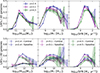 |
Fig. B.1. Fraction of intrinsic TNG100 LAEs relative to the total galaxy population, for the three redshifts: z = 2.4 (blue), z = 3.1 (magenta), and z = 4.5 (green). The LAE sample represents the intrinsic LAE population, not affected by our stochastic selection. Upper panel: Fraction of total LAEs relative to the total galaxy population as a function of different properties. Left: as a function of the halo mass, M200. Middle: dependence with stellar mass, M*. Right: as a function of the star formation rate (SFR). Shaded regions correspond to uncertainties, which were estimated based on the dispersion and by assuming Poisson errors. The trends indicate that LAEs preferentially reside in intermediate-mass halos, with moderate stellar masses and SFR, showing a consistent behavior across redshifts. Bottom panel: Same as the upper panel, but showing the fraction of LAEs separated into central galaxies (defined as those with the highest stellar mass within a halo, dotted lines) and satellite galaxies (dashed lines), relative to the total galaxy population in TNG100. |
Appendix C: Surface densities of Lyα and UV luminosities normalized by the virial area
As shown in the right panels of Figure 4, Figure C.1 shows the mean virial surface luminosities of Lyα (erg s−1 kpc−2, left panel) and UV (erg s−1 Hz−1 kpc−2, right panels) as a function of LAE multiplicity. In this case, the normalization is based on the area defined by the mean R200 (radius of the host halo whose mean density is 200 times the critical density of the Universe) obtained from the mock, applied to both mock and observations. The black lines correspond to the TNG100-true values, the pink lines to the TNG100-identified sample, and the cyan lines to the ODIN-COSMOS data, with solid, dashed, and dotted lines representing z = 2.4, z = 3.1, and z = 4.5, respectively. Error bars indicate the standard error of the mean in each bin. In most cases, higher LAE multiplicity is associated with enhanced surface brightness densities.
In the right panel, we also show the expected densities of halos without LAEs in blue for the three redshifts. These halos have radii within the ranges defined by the mean radii of the identified isolated systems, the pairs of LAEs, and the triplets of LAEs, including the corresponding data dispersion, respectively. We find that the same trend holds even for halos without Lyα emitters, indicating that our LAE-selected halos trace the UV density in an unbiased way.
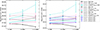 |
Fig. C.1. Mean virial surface luminosities of Lyα (erg s−1 kpc−2, left) and UV (erg s−1 Hz−1 kpc−2, right) as a function of LAE multiplicity. Normalization is based on the area defined by the mean R200 of the host halo. Black: TNG100-true; pink: TNG100-identified; cyan: ODIN-COSMOS; blue: halos without LAEs (see explanation in the text). Solid, dashed, and dotted lines correspond to z = 2.4, z = 3.1, and z = 4.5, respectively. Error bars show the standard error of the mean in each bin. |
All Tables
All Figures
|
Fig. 1. Lyman-alpha luminosity (left panels), REW (middle panels), and UV absolute magnitude (MUV, right panels) distributions per unit volume for redshifts z = 2.4 (top panels), z = 3.1 (middle panels), and z = 4.5 (bottom panels). The solid green line shows the ODIN-COSMOS LAE sample (Lyα Lum ≥ 1042 erg s−1 and REW ≥ 20 Å), while the shaded gray area shows the same sample in the TNG100 simulation. The solid blue line shows a randomly selected subset representing 25%, 33%, and 40% of the LAEs in TNG100 at z = 2.4, 3.1, and 4.5, respectively. The shaded pink areas show the latter samples applying a minimum luminosity cut of 1042.04, 1042.18, and 1042.37 erg s−1 (vertical dashed line shown in the left panels), respectively. The shaded orange areas show the REW distributions noisified by photometric uncertainties, while the sky blue shaded regions show the corresponding noisified MUV distributions (see text). |
| In the text | |
|
Fig. 2. Mean halo mass as a function of the number of LAEs within the halo at z = 2.4 (blue), z = 3.1 (magenta), and z = 4.5 (green). The TNG100 true multiples are shown with solid lines, while the TNG100 multiples identified using projected distances of rpmax = 100 pkpc at z = 2.4, 70 pkpc at z = 3.1 and 50 pkpc at z = 4.5 are displayed using dashed lines. Shaded regions and error bars show the error of the mean. As the number of LAEs in a halo increases, the true mean halo mass also increases, suggesting that the number of physically associated LAEs can serve as a proxy of halo mass. The identified multiples follow the underlying trend more closely at higher redshift. |
| In the text | |
|
Fig. 3. Mean Lyα luminosity (top panels) and UV magnitude (bottom panels) as a function of the LAE multiplicity for redshifts z = 2.4 (left), z = 3.1 (middle), and z = 4.5 (right). Solid black lines correspond to the TNG100-true multiples, dashed pink lines show the TNG-identified multiples (with rpmax = 100 pkpc at z = 2.4, 70 pkpc at z = 3.1, and 50 pkpc at z = 4.5), and dotted cyan lines correspond to the ODIN-COSMOS sample under the same selection criteria. The lighter black and pink lines indicate the mean UV magnitudes perturbed by photometric uncertainties for the mock samples. Error bars represent the standard error of the mean. Overall, both Lyα luminosity and UV magnitude tend to increase slightly with LAE multiplicity, supporting the idea that multiple LAEs trace more massive and actively star-forming halos. |
| In the text | |
|
Fig. 4. Virial surface brightness of Lyα (erg s−1 kpc−2) and UV (erg s−1 Hz−1 kpc−2) luminosities as a function of LAE multiplicity. Left panels: Mean virial surface luminosities for Lyα (top) and UV (bottom) emissions in TNG100, defined as the total luminosity per projected area, at z = 2.4 (blue), z = 3.1 (magenta), and z = 4.5 (green), plotted as a function of the fraction of LAEs relative to the total number of galaxies in the halo. Solid lines correspond to LAE-based densities, while dotted lines correspond to galaxy-based densities. Insets display the mean total luminosity before normalization. Error bars represent the standard error of the mean. Both Lyα and UV virial densities increase with the LAE fraction, reaching a peak at ∼0.5. This behavior is mainly driven by the Lyα model, which produces a more compact spatial distribution of LAE galaxies within halos. Right panels: Mean virial surface luminosities as a function of LAE multiplicity. Black lines show the TNG100-true values, pink lines show the TNG100-identified sample, and cyan lines are for the ODIN-COSMOS data. The solid, dashed, and dotted line styles denote z = 2.4, z = 3.1, and z = 4.5, respectively. Error bars represent the standard error of the mean in each bin. Higher LAE multiplicity appears to be associated with increased virial surface brightness densities. |
| In the text | |
|
Fig. 5. Distribution of minimum subhalo masses in the halos at z = 2.4 (left panel), z = 3.1 (middle panel), and 4.5 (right panel). In the top panels, the minimum subhalo mass distributions from TNG100 are shown as shaded black histograms, while the model predictions described in Section 5.3 are overplotted as dashed black lines (with fϕ = 0.11 and fM/fr = 2.43 at z = 2.4, fϕ = 0.39 and fM/fr = 0.78 at z = 3.1, and fϕ = 0.50 and fM/fr = 0.63 at z = 4.5). Using these factors, we test the model against all TNG100 LAEs (colored dashed lines in the top panels), TNG100 true 1 LAEs (dotted orange lines in the middle panels), and TNG100 true 2 LAEs (dash-dotted red lines in the bottom panels), comparing them with the corresponding minimum subhalo mass distributions of TNG100 LAES (shaded colored histograms). The model shows a good agreement with the minimum subhalo mass distribution for all galaxies, for all LAEs, and isolated LAEs, but struggles to reproduce as closely the distribution for LAE pairs. |
| In the text | |
|
Fig. A.1. Fraction of detections in which not all members belong to the same halo (contamination, left panel) and fraction of halos with at least two galaxies that are recovered (completeness, right panel), as a function of the maximum projected distance rpmax, for the mock samples at z = 2.4 (blue), z = 3.1 (magenta) and z = 4.5 (green). The total fractions are shown with solid lines, while the fractions corresponding multiples of 2 LAEs are shown with dashed lines, and multiples of 3 LAEs with dotted lines. Both the contamination and the fraction of recovered halos increases with the rpmax, so it is necessary to find a compromise value between them. |
| In the text | |
|
Fig. B.1. Fraction of intrinsic TNG100 LAEs relative to the total galaxy population, for the three redshifts: z = 2.4 (blue), z = 3.1 (magenta), and z = 4.5 (green). The LAE sample represents the intrinsic LAE population, not affected by our stochastic selection. Upper panel: Fraction of total LAEs relative to the total galaxy population as a function of different properties. Left: as a function of the halo mass, M200. Middle: dependence with stellar mass, M*. Right: as a function of the star formation rate (SFR). Shaded regions correspond to uncertainties, which were estimated based on the dispersion and by assuming Poisson errors. The trends indicate that LAEs preferentially reside in intermediate-mass halos, with moderate stellar masses and SFR, showing a consistent behavior across redshifts. Bottom panel: Same as the upper panel, but showing the fraction of LAEs separated into central galaxies (defined as those with the highest stellar mass within a halo, dotted lines) and satellite galaxies (dashed lines), relative to the total galaxy population in TNG100. |
| In the text | |
|
Fig. C.1. Mean virial surface luminosities of Lyα (erg s−1 kpc−2, left) and UV (erg s−1 Hz−1 kpc−2, right) as a function of LAE multiplicity. Normalization is based on the area defined by the mean R200 of the host halo. Black: TNG100-true; pink: TNG100-identified; cyan: ODIN-COSMOS; blue: halos without LAEs (see explanation in the text). Solid, dashed, and dotted lines correspond to z = 2.4, z = 3.1, and z = 4.5, respectively. Error bars show the standard error of the mean in each bin. |
| In the text | |
Current usage metrics show cumulative count of Article Views (full-text article views including HTML views, PDF and ePub downloads, according to the available data) and Abstracts Views on Vision4Press platform.
Data correspond to usage on the plateform after 2015. The current usage metrics is available 48-96 hours after online publication and is updated daily on week days.
Initial download of the metrics may take a while.