| Issue |
A&A
Volume 706, February 2026
|
|
|---|---|---|
| Article Number | A253 | |
| Number of page(s) | 16 | |
| Section | Galactic structure, stellar clusters and populations | |
| DOI | https://doi.org/10.1051/0004-6361/202557098 | |
| Published online | 17 February 2026 | |
Beyond the Clouds: S3 as the most distant extended Milky Way stream, not of LMC origin
1
Lund Observatory, Division of Astrophysics, Department of Physics, Lund University,
Box 43,
22100
Lund,
Sweden
2
Institute for Computational Cosmology, Department of Physics, Durham University,
South Road,
Durham
DH1 3LE,
UK
3
Institute for Astronomy, University of Edinburgh,
Royal Observatory Edinburgh, Blackford Hill,
Edinburgh
EH93HJ,
UK
★ Corresponding author: This email address is being protected from spambots. You need JavaScript enabled to view it.
Received:
4
September
2025
Accepted:
13
December
2025
Abstract
Context. While the influence of the LMC on Milky Way (MW) stellar streams has been extensively studied, streams associated with the Clouds have received far less attention. Beyond the Magellanic Stream, only four stream candidates (S1–S4) have been reported.
Aims. We focus on the S3 stream, a long (~30°) and narrow (~1.2°) structure at 60–80 kpc that is nearly aligned with the LMC. Our goals are: (1) to validate the stream through a kinematic analysis of S3 candidates with Gaia DR3 data; (2) to enlarge the sample of potential members with machine-learning methods; and (3) to model the stream in order to test its association with either the MW or the LMC.
Methods. We selected new S3 candidates with a supervised neural network classifier trained on Gaia DR3 astrometry and photometry, and further reduced contamination through a polygon cut in the proper-motion space. To investigate the origin of S3, we evolved stream models within time-dependent, deforming MW and LMC halos, thereby accounting for possible effects of the MW–LMC interaction.
Results. We identify 1542 high-confidence new S3 stream candidates and find that the stream’s apparent width has grown from ~1.2° to ~3–4° compared to previous studies. We also present a list of 440 potential S3 red clump stars, which are valuable targets for spectroscopic follow-up thanks to their well-defined luminosities and ability to yield precise distances. Both modelling and a comparison of S3 stars’ closest approach distance and velocity with the LMC’s escape velocity indicate that S3 likely does not originate from the LMC and instead represents a distant (~75 kpc) MW stream.
Conclusions. S3 is the most distant (~75 kpc) extended (~30° long, ~3–4° thick) MW stream known, offering a unique probe of the outer halo and the LMC’s recent influence. Its angular width corresponds to a physical thickness of ~4–5 kpc, making S3 among the thickest streams discovered.
Key words: Galaxy: halo / Galaxy: kinematics and dynamics / Magellanic Clouds / galaxies: structure
© The Authors 2026
 Open Access article, published by EDP Sciences, under the terms of the Creative Commons Attribution License (https://creativecommons.org/licenses/by/4.0), which permits unrestricted use, distribution, and reproduction in any medium, provided the original work is properly cited.
This article is published in open access under the Subscribe to Open model. This email address is being protected from spambots. You need JavaScript enabled to view it. to support open access publication.
1 Introduction
Stellar streams are elongated structures of stars that originate from the tidal disruption of globular clusters or dwarf galaxies as they interact with the gravitational potential of the host galaxy. These coherent structures are among the most powerful tracers of the host galaxy’s assembly history and its dark matter distribution (e.g. Springel & White 1999; Dubinski et al. 1999; Johnston et al. 1999, 2005; Binney 2008; Koposov et al. 2010; Law & Majewski 2010; Price-Whelan et al. 2014; Erkal et al. 2016; Bovy et al. 2016; Shipp et al. 2021; Pearson et al. 2022b; Koposov et al. 2023; Ibata et al. 2024). In the Local Universe (e.g. Martínez-Delgado et al. 2010; Bílek et al. 2020; Martínez-Delgado et al. 2023; Miró-Carretero et al. 2024; Martínez-Delgado et al. 2025) and beyond (e.g. Kado-Fong et al. 2018), dozens of tidal streams have been found thanks to facilities designed to detect low-surface-brightness features.
Closer, in our own Galaxy, the Milky Way (MW), we now count nearly 150 candidate stellar streams (Mateu 2023), with an explosion of stream discoveries over the past decade from surveys such as the Dark Energy Survey (DES; The Dark Energy Survey Collaboration 2005), the Sloan Digital Sky Survey (SDSS; Kollmeier et al. 2017, 2026), and, in particular, the Gaia mission (Gaia Collaboration 2018, 2021a, 2023). Thanks to Gaia, over the past 10 years, we have not only increased the number of known MW streams, but also, for the first time, uncovered their kinematics. This constrains their exact orbits as well as the origins and the complex structure of stellar streams, which point to dynamical histories shaped by significant perturbations. In the future, we anticipate that telescopes like the Vera Rubin Observatory (Ivezić et al. 2019) and the Nancy Grace Roman Space Telescope (Spergel et al. 2015) will find dozens more streams in both the MW and external galaxies (e.g. Pearson et al. 2022a, 2024; Bonaca & Price-Whelan 2025).
When detecting stellar streams, the primary difficulty comes from their intrinsic low stellar densities and brightness, which make them challenging to observe and study. Historically, the central approach to locating and characterising stellar streams focused on enhancing contrast against the foreground MW stars – either by targeting rare tracers more commonly associated with streams than with the field or by filtering datasets to boost the relative presence of stream stars. This approach, which focused on photometric data from the Galactic halo – where the background stellar density is naturally lower than in the disc or central regions – enabled the discovery of the first stellar streams and substructures around the Galaxy (e.g. Rockosi et al. 2002; Newberg et al. 2002; Grillmair & Dionatos 2006; Belokurov et al. 2006).
However, even though a stream can be detected using matched filtering on photometry alone, its density is usually not well constrained because the stream stars are frequently low signal-to-noise features over the background stellar density. Shortly after Gaia Data Release 2 (DR2), Price-Whelan & Bonaca (2018) demonstrated the power of combining kinematic and photometric data to identify stream members and estimate a stream’s density in the MW – applying this approach specifically to the GD-1 stream. They showed how the exceptional astrometric precision provided by Gaia enabled the development of a wide range of methods for probing the density structure of known streams (e.g. Koposov et al. 2019; Ferguson et al. 2022; Tavangar et al. 2022; Patrick et al. 2022; Starkman et al. 2023; Tavangar & Price-Whelan 2025) and paved the way for an entirely new class of techniques dedicated to discovering previously unknown streams in the MW’s halo (e.g. Malhan & Ibata 2018; Borsato et al. 2020; Necib et al. 2020; Gatto et al. 2020; Shih et al. 2022; Pettee et al. 2024). All of these methods take advantage of the kinematic data provided by Gaia to identify stellar over-densities across various projections or transformations of phase-space.
Moreover, the advent of Gaia kinematics has not only enabled the discovery of numerous new stellar streams, but has also provided a powerful means to reassess and validate previously identified ones with unprecedented precision. Among the most compelling and overlooked environments for such studies are the LMC and the SMC (collectively referred to as ‘the Clouds’ in this paper), located at a distance of approximately 50–60 kpc (Graczyk et al. 2014; Pietrzyński et al. 2019). As the most massive satellite galaxies of the MW, the Clouds offer a valuable opportunity to explore a range of dynamical phenomena. These include tidal interactions (e.g. Besla et al. 2012; Vasiliev 2024; Jiménez-Arranz et al. 2024b; Jiménez-Arranz & Roca-Fàbrega 2025), dynamical perturbations (e.g. Vasiliev 2018; Jiménez-Arranz et al. 2023b; Kacharov et al. 2024; Jiménez-Arranz et al. 2024a, 2025; Rathore et al. 2025; Schölch et al. 2025), and stream formation (e.g. Nidever et al. 2008; Lucchini et al. 2020, 2021; Chandra et al. 2023; Zaritsky et al. 2025). Crucially, the Clouds occupy a regime that is external to the MW yet close enough to allow detailed studies of resolved stellar populations and coherent dynamical structures.
While a considerable amount of effort has been devoted to understanding the impact of the LMC on the dynamics and morphology of MW stellar streams (e.g. Erkal et al. 2019; Koposov et al. 2019; Shipp et al. 2021; Vasiliev et al. 2021; Koposov et al. 2023; Lilleengen et al. 2023; Brooks et al. 2024), comparatively little work has focused on the streams that are themselves associated with the LMC and SMC. To the best of our knowledge, only four potential stellar streams associated with the Clouds have been reported in the literature – besides the well-known Magellanic Stream (e.g. Bajaja et al. 1985; Putman 2000; Putman et al. 2003; Nidever et al. 2008; D’Onghia & Fox 2016; Lucchini et al. 2021; Petersen et al. 2022a; Chandra et al. 2023; Zaritsky et al. 2025). In a seminal study, Belokurov & Koposov (2016, hereafter BK16) identified several narrow stellar streams and diffuse debris clouds, cataloguing the (four) most prominent – labelled S1 to S4 according to the distance modulus bin they occupy – by applying photometric filtering to blue horizontal branch (BHB) stars detected in DES (Diehl et al. 2014; Koposov et al. 2015). Following up on BK16, Navarrete et al. (2019, hereafter N19) conducted a spectroscopic follow-up programme of the four stellar stream candidates; only two of the four (S1 and S2) were confirmed to have an LMC or SMC origin. Discovered in the pre-Gaia era (2016, prior to Gaia DR2 in 2018), these streams have since been largely overlooked by the community, with no follow-up studies incorporating astrometric data to date.
In this work, we built upon these previous analyses, focusing on the S3 stream, a long (~30°) and narrow (~1.2°) stream at distances ranging from 60 to 80 kpc that points nearly exactly in the direction of the LMC. We pursued three primary objectives: (1) to extend the kinematic analysis of the S3 stellar candidates identified by N19 by incorporating astrometric data from Gaia Data Release 3 (DR3), with the goal of reassessing and validating the stream’s existence; (2) to expand the sample of potential S3 members using machine learning techniques; and (3) to generate stream models to determine S3’s association with either the MW or the LMC and to gain a better understanding of the data and future observation needs.
This paper is organised as follows: in Sect. 2 we describe the datasets used to (kinematically) confirm the existence of the S3 stellar stream. In Sect. 3, we present the methodology developed to identify new candidate members using machine learning techniques and to characterise the expanded sample of S3 candidates. In Sect. 4, we present stream models to better understand discrepancies in the data and to confirm that S3 is a MW stream. In Sect. 5, we contextualise and discuss our results. Finally, in Sect. 6 we summarise the main conclusions of this work.
2 Data
In this work, we made use of two distinct datasets. In Sect. 2.1 we present the S3 candidates from N19. In Sect. 2.2, we describe the Gaia DR3 bulk catalogue, which we used both to kinematically confirm the existence of the stream and to identify new S3 candidates (see Sect. 3.1).
Hereafter, every on-sky density figure is displayed in the orthographic projection (x, y, vx, vy) – namely, a method of representing 3D objects where the object is viewed along parallel lines that are perpendicular to the plane of the drawing – of the usual celestial coordinates (α, δ) and proper motions (μα*, μδ), centred in the LMC photometric centre, defined as (αc, δc) = (81.28°, −69.78°) by van der Marel (2001). Please refer to Eqs. (1) and (2) of Gaia Collaboration (2021b) and Fig. 11 of Jiménez-Arranz et al. (2023b) for additional details on the coordinate transformation.
2.1 BHB and BS S3 candidates from N19
The detection of an extended and lumpy stellar debris distribution around the Clouds was reported by BK16 using BHB stars found in DES Year 1 data. The authors of that work reported the discovery of several narrow streams and diffuse debris clouds, and they catalogued the (four) most important of the stellar substructures that were discovered – labelled from S1 to S4 according to the distance modulus bin they occupy. Among them, the BHB stars traced the long (~30°) and narrow (~1.2°) S3 stream, at distances ranging from 60 to 80 kpc, which runs along the great circle with the pole at (α, δ) = (250.15°, 152.35°) and points nearly exactly in the direction of the LMC. In that work, the authors postulated that the S3 stream could conceivably be a by-product of the LMC–SMC interaction because of its alignment with the proper motion of the Clouds and its overlap with its gaseous Stream.
As a logical extension of the project, and using the medium-resolution spectrograph FORS2 installed at the Very Large Telescope (VLT), N19 conducted a spectroscopic follow-up programme of the four stellar stream candidates found on the outskirts of the LMC by BK16. In that work, a quarter of the stellar stream candidates (25 out of 104) were found to be contaminants, primarily white dwarfs and quasi-stellar objects (QSOs). However, for the other 79 stellar stream candidates, the authors used the Balmer lines to create a classification system that distinguished the BHB stars from blue stragglers (BSs). According to their classification, 24 stars are of BHB type, 45 are BSs, and 10 have uncertain classification.
In this study we began with a sample of 11 BHB and BS stars identified as members of the S3 stream associated with the Clouds (labelled ‘MCs-M1’ or ‘MCs-M2’ in Table 1 of N19). This classification, originally proposed by N19, is based exclusively on distance and should therefore be interpreted with caution. After crossmatching with Gaia DR3 data (see Sect. 2.2), we removed one source (S3 05) that exhibited near-zero proper motion (μα*, μδ) ~ (0, 0) mas yr−1, which is indicative of still potential QSO contamination. This sample of 10 S3 stellar candidates, consisting of BHB and BS stars identified by N19, is first used to reassess and kinematically confirm the presence of the stream using Gaia DR3 data (see Sect. 2.2), and subsequently serves as the training set for identifying additional S3 candidates (see Sect. 3.1). The top panel of Fig. 1 displays the on-sky distribution of the clean S3 candidates (orange circles) from N19. This figure highlights the directionality and grouping of its member stars and demonstrates how the stream structure is coherent in density.
It is important to acknowledge some limitations of the N19 dataset. First, the classification between BHB and BS stars is uncertain, which directly impacts the inferred distances (see Sect. 5 for more details). Additionally, the reported line-of-sight velocities exhibit significant variation (see Fig. 10 of N19) that cannot be fully accounted for at this stage. While these issues introduce some ambiguity, we defer a detailed treatment to the modelling section (see Sect. 4), where we show that, across a reasonable range of line-of-sight velocity assumptions, the stars still trace a coherent stream.
2.2 Gaia DR3 data: Kinematic confirmation of the S3 stream
Building on the spectroscopic efforts of N19, which provided missing line-of-sight velocity measurements for stars scattered across the outskirts of the LMC identified by BK16, our study has two main objectives. First, we used Gaia DR3 data to incorporate proper motion information for the known S3 stellar candidates in order to reassess and validate the existence of the stream (see later in this section). Second, we aimed to identify new S3 candidates within the Gaia dataset (see Sect. 3.1).
The Gaia mission is a primarily astrometric (with also photometric and spectroscopic instruments) survey whose main goal is to create the most precise and detailed 3D map of our Galaxy. Insofar, it has catalogued and determined astrometric and photometric data for almost two billion stars (Gaia Collaboration 2016, 2018, 2021a, 2023), representing around 1% of all stars of the MW. Among the vast number of sources observed by Gaia, approximately 15 million stars are associated with the Clouds (Jiménez-Arranz et al. 2023a,b). This dataset has proven effective for investigating the internal kinematics of the LMC (e.g. Jiménez-Arranz et al. 2023b; Navarrete et al. 2023; Jiménez-Arranz et al. 2024a; Kacharov et al. 2024; Dhanush et al. 2024; Jiménez-Arranz et al. 2025; Rathore et al. 2025). Within the field of view considered in this study (see Fig. 1), there are approximately 28 million Gaia DR3 stars, comprising both stars from the Clouds and MW foreground halo stars. This Gaia DR3 sample forms the background for the two panels shown in Fig. 1.
We crossmatched the sample of 10 BHB and BS stars identified by N19 as potential S3 stream members (see Sect. 2.1) with the Gaia DR3 catalogue. We used this sample aiming to reassess and kinematically confirm the presence of the stream structure. Figure 1 (top panel) displays the on-sky distribution of the clean S3 candidates (orange circles), with arrows indicating their respective proper motions. The orientation and length of the arrows represent the direction and magnitude of the stars’ motion across the sky. This visualisation underscores both the spatial alignment and the coherent motion of the candidate members, illustrating that the stream is not only continuous in position but also coherent in proper motion space. The consistency in their motion provides strong kinematic evidence that S3 is a genuine stellar stream.
3 Identification of new S3 candidate members with Gaia data
In this section we present the methodology developed to identify new S3 candidate members within the Gaia DR3 dataset (see Sect. 2.2) and to characterise the expanded candidate sample. First, in Sect. 3.1 we introduce the neural network classifier used for the initial selection of new S3 candidate stars. Then, in the same section we examine the proper motion space of these candidates and identify an additional cut in the proper motion space that helps remove potential contaminants, yielding the final new list of 1542 S3 candidates based on Gaia data. Finally, in Sect. 3.2 we characterise the new resulting sample of highly reliable S3 stream candidates.
3.1 Neural network classifier and polygon selection in the proper motion space
Since our goal is to develop a classifier capable of identifying stars belonging to the S3 stream within the Gaia DR3 sample (see Sect. 2.2), we employed a machine learning approach – specifically, supervised learning. We emphasise that the neural network approach used in this work is not intended to provide a physical model of the stream, but rather serves as a practical tool for defining a multi-dimensional separation in a parameter space where manual tuning would be challenging.
Supervised learning requires a well-constructed, labelled training sample so that the classifier can learn to distinguish the characteristics of stars associated with the S3 stream from field stars. As introduced earlier in the manuscript, the training sample combines the 10 S3 stellar candidates – composed of BHB and BS stars identified by N19 (see Sect. 2.1) – with stars from the Gaia DR3 catalogue (see Sect. 2.2). Given the strong imbalance between the two datasets (10 stars vs 28 million stars), we replicated the S3 sample 20 times. While this procedure does not add new information and cannot mitigate the inherent uncertainty of such a small sample, it provides a simple way to reduce the class imbalance during training. From the Gaia DR3 catalogue, we randomly selected a subsample of 10 000 stars to represent the field population. While it is possible that a small number of genuine S3 members are be included in this sample, their presence is expected to be negligible and unlikely to significantly affect the performance of the classifier. The results in this work have been confirmed to be robust against reasonable variations in these sample sizes.
The neural network architecture employed in this work closely follows the design used by Jiménez-Arranz et al. (2023a,b). It consists of 11 input neurons, corresponding to 11 parameters either derived from or directly measured by Gaia (detailed below), and three hidden layers containing six, three, and two nodes, respectively. The network outputs a single value, P, representing the probability that a given star belongs to the S3 stream. A probability close to 1 indicates a high likelihood of S3 membership, whereas a value near 0 suggests the star is more likely associated with the MW halo or the Clouds. The activation function used in all hidden layers is the rectified linear unit (ReLU), and the model is optimised using the ‘adam’ stochastic gradient descent algorithm (Kingma & Ba 2017), with a constant learning rate. Training is performed by minimising the log-loss function, and to mitigate overfitting, we applied L2 regularisation with a strength of 1e-5.
As input variables, we used the orthographic positions (x, y), parallax and its uncertainty (ϖ, σϖ), orthographic proper motions and their uncertainties1 (vx, vy, σvx, σvy), and Gaia photometry (G, GBP, GRP). After testing various coordinate systems for the neural network input – such as equatorial coordinates (α, δ, μα*, μδ) and galactocentric coordinates (l, b, μl, μb) – we chose to adopt the orthographic projection (x, y, vx, vy). This choice avoids issues associated with coordinate singularities at the poles, which affected both the equatorial and galactocentric systems, and resulted in better performance for the classifier. The SKLEARN Python package (Pedregosa et al. 2011) was used to create the S3 classifier.
To convert the classifier’s output probabilities into a binary classification, we had to define a probability threshold. Then, a star is considered a candidate member of the S3 stream if its probability exceeds this threshold, i.e. P > Pcut. Choosing a lower Pcut increases completeness by ensuring that few, if any, true S3 members are missed, but this comes at the expense of higher contamination from non-members (field stars). In contrast, a higher threshold improves the purity of the selected sample by reducing contaminants, though it risks excluding genuine S3 stars and thus lowers completeness. In this work we adopted Pcut = 0.8 as our priority is to obtain a cleaner, less contaminated sample of S3 candidates, even at the cost of missing some true members2. However, the main results of this work remain unchanged across the probability threshold range of Pcut = 0.5–0.8. We refer the reader to Appendix A for the on-sky distribution of the S3 clean samples when using Pcut = 0.5.
To train and evaluate the performance of the classifier, we split the sample of 10 200 stars (including both S3 and field stars) into two subsets: 60% for training the algorithm and 40% for testing it. The classifier’s performance is assessed by computing the receiver operating characteristic (ROC) curve, the precision-recall curve, and their respective areas under the curve (AUCs). All these metrics indicate an almost perfect classifier – see Appendix B for full details. Nonetheless, these results should be interpreted with caution, as they reflect performance on the test portion of our simulated sample, not on the full Gaia DR3 dataset. In addition, also in Appendix B, we present an analysis of the SHAP (SHapley Additive exPlanations) values to gain insight into the internal decision-making process of the classifier and to better understand the contribution of each feature to the model’s output.
When applied to the Gaia DR3 sample (28 million sources; see Sect. 2.2), the neural network classifier identifies 25 536 potential S3 stream candidates (beige circles in the top panel of Fig. 1). The spatial distribution of these candidates shows a reasonable alignment with the BHB–BS training sample from N19 (orange circles; see Sect. 2.1). However, their proper motion vectors are not well aligned with the stream track or with those of the training sample. Figure 2 compares the proper motion distribution of the BHB–BS S3 training sample from N19 (orange circles) with that of the newly identified S3 candidates selected by the neural network (beige and red transparent circles). In the newly identified S3 candidates sample, we observe two distinct overdensities. The first, centred around (μα*, μδ) ~ (1, −1) mas yr−1, is consistent with the expected kinematics of the S3 stream. While there is some overlap with the kinematics of the SMC, the implications of this are addressed in Sect. 5. The second (and more prominent) overdensity, located near (μα*, μδ) ~ (0, 0) mas yr−1, is not associated with the stream and likely represents contamination from unrelated field stars – or QSOs, which typically exhibit very small proper motions.
This contaminating component is filtered out to produce a cleaner and more reliable sample of S3 candidates by applying a polygon selection in the proper motion space (dashed black and white line), computed from a convex hull encompassing the 1 − σ uncertainties of all S3 members’ of the training sample to define the region occupied by more reliable stream members. After applying the polygon selection in proper motion space, we retain 1542 highly reliable (P > 0.8) S3 stream candidates (beige circles). This is the refined sample that we characterise in Sect. 3.2 and use for modelling in Sect. 4.
We compared the neural network with analytic classifiers, specifically linear discriminant analysis (LDA) and a Mahalanobis distance model, using identical input features and training labels. In the presence of strong class imbalance, the neural network (precision-recall area under the curve, PR-AUC = 0.982; see the bottom panel of Fig. B.1) significantly outperforms both LDA and Mahalanobis classifiers, which achieve PR-AUC values of 0.464 and 0.034, respectively. While LDA shows moderate performance on a small test set, it fails to recover the stream in the full Gaia dataset, and the Mahalanobis approach essentially fails. The neural network’s flexible, piecewise-linear boundary effectively traces the stream in parameter space, highlighting its practical advantage over traditional analytic methods.
The bottom panel of Fig. 1 shows the on-sky distribution of the newly identified S3 candidates (beige circles) using both the neural network classifier and a polygon selection in proper motion space, where the arrows’ orientation and length indicate the direction and magnitude of the stars’ motion across the sky. In comparison to the neural network classifier only (top panel), we can see that the stream-like spatial distribution is preserved while the proper motions are more aligned to the stream track – except the part closer to the LMC, at the left of the stream, where the proper motion of the new S3 candidates do not align with the training sample.
We observe a significant increase in the apparent width of the S3 stream compared to previous studies. In BK16, S3 stream stars are traced out to ~1.2°, while in this work we identify members extending up to ~3°, and in some regions as wide as ~4°. In N19, the S3 stream appears even narrower, but this is likely a consequence of selection effects inherent to the spectroscopic sample. A key factor contributing to the broader extent in our analysis may be the difference in selection methodology. BK16 relied on photometric criteria targeting specific stellar types such as BHB and BS stars, which naturally limited the sample. In contrast, our neural network approach is more inclusive, allowing a wider range of stellar populations to be identified (see Sect. 3.2), potentially revealing a more complete and extended picture of the stream. If this broader structure is confirmed, S3 would rank among the thickest stellar streams discovered to date, with an apparent width of up to ~3–4°. At the median distance of the S3 training sample (~73.5 kpc), this corresponds to a physical thickness of ~4–5 kpc.
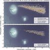 |
Fig. 1 Comparison of the on-sky distribution of the N19’s BHB–BS S3 training sample (orange circles) to the newly identified S3 candidates (beige circles), shown in the top panel using the neural network classifier alone, and in the bottom panel using both the neural network classifier and a polygon selection in proper motion space (see Sect. 3.1). The arrows’ orientation and length indicate the direction and magnitude of the stars’ motion across the sky, with a 2 mas yr−1 white arrow shown as a reference in the bottom panel. For the newly identified S3 candidates, we computed the median direction and magnitude of their motion across the sky within 1.6 × 1.6 deg2 bins, displaying the results only for bins containing more than 20 stars. The black arrows indicate the systemic motion of the LMC and SMC. The background image corresponds to a 2D histogram of the Gaia DR3 sample utilised in this study (see Sect. 2.2), consisting of 28 million stars that include both stars from the Clouds and foreground halo stars of the MW. Both panels are displayed using the orthographic projection (x, y, vx, vy) of the standard celestial coordinates (α, δ) and proper motions (μα*, μδ), centred in the LMC photometric centre, defined as (αc, δc) = (81.28°, −69.78°) by van der Marel (2001). |
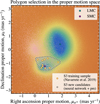 |
Fig. 2 Comparison of the proper motion distribution between the BHB–BS S3 training sample from N19 (orange circles) and the newly identified S3 candidates (beige and red transparent circles), overlaid on the Gaia DR3 sample (background histogram; see Sect. 2.2). The dashed black and white line indicates the polygon selection applied in proper motion space (see Sect. 3.1). The newly identified S3 candidates are shown in beige if they lie inside the polygon selection, and in transparent red if they fall outside it. The cyan and magenta crosses indicate the systemic motions of the LMC and SMC, respectively. In the background, regions of higher (lower) density are shown in bluer (redder) colour. |
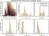 |
Fig. 3 Characterisation of the refined sample of 1542 new S3 stellar candidates (see Sect. 3.1). Top left panel: CMD of the S3 training sample by N19 (orange circles) and the new S3 candidates (beige circles). The background image corresponds to the CMD of the Gaia DR3 sample utilised in this study (see Sect. 2.2). Top centre and right panels: proper motion normalised distributions in right ascension (μα*) and declination (μδ), respectively. Bottom from left to right: parallax (ϖ) and proper motion error normalised distributions in right ascension (σμα*) and declination (σμδ). In the histograms, the S3 training sample from N19 is shown in orange and the new S3 candidates in beige. |
3.2 Characterisation of the new S3 candidate sample
In this section we analyse the refined sample of 1542 new S3 stellar candidates, identified through the combined application of the neural network classifier and a polygonal selection in proper motion space. The top panel of Fig. 3 compares the colour-magnitude diagram (CMD) of the training sample by N19 (orange circles) with the new 1542 S3 candidates (beige circles). We observe that the training sample is concentrated around GBP − GRP ~ 0–0.5 and G ~ 20, as expected given its composition of BHB and BS stars. However, the first step of our selection process – the neural network classifier – successfully generalises the search for new S3 stars, identifying candidates belonging to a broader range of stellar populations. When compared to the LMC evolutionary phases proposed in Gaia Collaboration (2021b), shifted to a distance of ~73.5 kpc – the median distance of the N19 training sample – we find that the sample of 1542 new S3 stellar candidates is (as a first indication) predominantly composed of red clump (RC; 29%) and RR Lyrae (25%) stars – further details are provided in Appendix C. We consider the overdensity at GBP − GRP ~ 1.5 and G ~ 19–20.5 to be of particular interest, as it may correspond to the RC population of the S3 stream, an especially valuable target for spectroscopic follow-up due to the RC stars’ well-defined luminosities and their potential to provide precise distance measurements3 (see further discussion in Sect. 5.2). Given that the CMD polygon cut proposed by Gaia Collaboration (2021b) indicated the possible presence of RR Lyrae stars within our S3 clean sample, we attempted to crossmatch this sample with the Gaia DR3 RR Lyrae catalogue (gaiadr3.vari_rrlyrae; Clementini et al. 2023), aiming to identify any overlap between the datasets. However, we found only 3 (7) RR Lyrae stars at distances greater than 50 kpc within the neural network S3 sample after (before) applying the proper motion cut. The distances are computed using the absolute magnitude derived in Iorio & Belokurov (2021), with approximate uncertainties of 10%. The individual distances of those 3 RR Lyrae stars are 60,55, and 73 kpc, placing some of them on the nearer side of the S3 stream. We refer the reader to Appendix D for details.
The top centre and right panels of Fig. 3 show the proper motion normalised distributions in right ascension (μα*) and declination (μδ), respectively. We can observe that the proper motion distribution of the new S3 candidates appears smoother and more Gaussian-like, closely resembling that of the training sample. The bottom left panel shows the parallax ϖ distribution where, again, the new S3 candidates show a Gaussian-like distribution. Finally, the bottom centre and right panels proper motion error normalised distributions in right ascension (σμα*) and declination (σμδ), respectively. Here, we observe that the training sample is clustered around σμα* and σμδ ~ 0.5 mas yr−1, whereas the new S3 sample exhibits a tail extending up to approximately ~2 mas yr−1.
4 Association of the distant S3 stream with the MW through dynamical modelling
Although the data are too sparse to confidently fit the stream, dynamical stream models can be used to gain a better understanding of the stream. To explore the association of the stream with either the MW or the LMC, and possible effects by either galaxy on the stream, we created models following a similar approach as Lilleengen et al. (2023, hereafter L23). We evolved the stream models in time-dependent and deforming MW and LMC potentials to take into account possible effects of the MW–LMC interaction (see e.g. Erkal et al. 2019; Garavito-Camargo et al. 2019; Petersen & Peñarrubia 2020; Garavito-Camargo et al. 2021; Petersen & Peñarrubia 2021; Petersen et al. 2022a; Koposov et al. 2023; Arora et al. 2024; Brooks et al. 2024, 2025, 2026; Weerasooriya et al. 2025; Yaaqib et al. 2025; Chandra et al. 2025).
4.1 Modelling approach
The MW–LMC simulation is evolved using the EXP method (Petersen et al. 2022b; Petersen & Weinberg 2025), where potential and density are modelled as a sum of orthogonal basis functions with an associated weight quantifying the contribution of the function to the total system. The coefficients vary over time to describe the time-dependent system, while the functions remain constant. This provides tabulated, i.e. fast and lightweight, access to force-replay for integrating orbits. The simulation consists of three components: the MW halo, the MW stellar component (disc and bulge), and the LMC halo. Further details are provided in L23, and access to the simulation is available through a dedicated Python package4.
We created a set of stream models using the modified Lagrange cloud stripping technique (Gibbons et al. 2014; Erkal et al. 2019). The progenitor is modelled as a Plummer sphere with a range of masses between 105 and 107 M⊙ and scale radii between 0.001 and 0.1 kpc. Present-day phase-space coordinates for the progenitor were estimated from the N19 candidates and the potential members identified in Sect. 3. We set the present-day phase-space position of the progenitor at fixed α = 18°, δ = −50°, μα* = 0.5 mas yr−1, μδ = −1.0 mas yr−1. The stream’s distance and radial velocities are more uncertain as discussed in Sect. 2.1 – Figure 4 shows the N19 candidates as white points, with distances and radial velocities in the second and third row, respectively. We tested two distances for the stream: 75 kpc, as indicated by the BHB stars, and 45 kpc, the approximate mean distance of the BS stars. The N19 line-of-sight velocities (vlos) are converted into Galactic standard of rest radial velocities (vgsr) using ASTROPY (Astropy Collaboration 2013, 2018, 2022) conversions. Since there is no clear trend in vgsr (see the third row in Fig. 4), we tried five values for the progenitor that are in the regime of the data: vgsr ∈ {200, 50, 0, −50, −100} km s−1. A coordinate system aligned with the stream provides the stream track coordinates (ϕ1, ϕ2). It follows a great circle with a pole at (αS3, δS3) = (18°, 40°) and has its origin at (α0, δ0) = (18°, −50°), which we chose as the progenitor’s position.
The progenitor is rewound in the time-evolving MW–LMC potential for 4 Gyr. Then, the system is evolved forwards, with tracer particles being released from the progenitor’s Lagrange points, generating a stream. These Lagrange points are generally calculated with respect to the MW, but with the possibility of S3 being an LMC stream, we also calculated them with respect to the LMC in another run. However, given the results presented in the remainder of this section, we did not further explore streams evolved around the LMC. A more in-depth description of the modelling approach is provided in L23.
4.2 Modelling results
4.2.1 Distance comparison and radial velocities
We present models with a progenitor mass of 107 M⊙ and a scale radius of 0.1 kpc, as these best match the observed ranges. Figure 4 shows the stream observables for all generated models stripping around the MW as coloured points, BHB stars and BS stars from N19 as white circles and squares, respectively, and new candidates as grey points. The newly identified candidates do not have any radial velocity measurements and only unresolved parallaxes, i.e. no reliable distance measurements. The colours of the models are set by the progenitors’ Galactic standard of rest radial velocities, ranging from 200 km s−1 in light pink to −100 km s−1 in dark blue. The left column shows streams at larger distances with the progenitors initialised at 75 kpc, and the right column shows streams at smaller distances with the progenitors at 45 kpc. This addresses the ambiguity in the data between the BHB and BS streams.
None of the models exactly match the data; however, they still help us understand more about the S3 stream and inform follow-up observations that will enable stream fitting. While the streams at larger distances match the data, particularly with progenitor radial velocities of 50 and 0 km s−1 (light and dark purple points in the third row in Fig. 4), streams at closer distances have a turning point near the progenitor and fail to produce streams that cover the whole data range. This is because the progenitors at smaller distances are near apocentre, with pericentres close to the MW centre, shown in Fig. 5.
The observed radial velocities (white points and squares) do not follow any of the models, which show a strong gradient along the stream. None of the models at either distance can explain the variety in the observations. To confirm S3 as a stream, we need spectroscopic follow-up observations to obtain radial velocities of the new S3 candidates provided by the neural network.
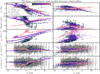 |
Fig. 4 Observables of S3 BHB and BS data from N19 (white points and squares, respectively, with black error bars), neural network candidates (grey points and error bars), and the stream model (coloured points). The rows show the stream track, its heliocentric distance, radial velocity in the Galactic standard of rest, and proper motions, not reflex-corrected, respectively. The left (right) column shows model streams with a progenitor distance of 75 kpc (45 kpc). The colours refer to the progenitor’s Galactic standard of rest radial velocities (see the colour bar in the top-left panel). The streams at the larger distance (75 kpc) match the data well, particularly with a radial velocity of 50 km s−1. The closer progenitors (45 kpc) fail to produce streams that cover the whole range of all observables in ϕ1. |
4.2.2 Is S3 a MW or LMC stream?
Figure 5 shows the distances between the progenitor and the MW (top panel) and the LMC (bottom panel). All progenitors are bound to the MW, with longer orbital periods for the farther streams and shorter orbital periods for the closer streams. They have their closest approach to the LMC around 100 Myr ago, where the closest distances for the farther streams are a few tens of kiloparsecs. Figure 4 shows that S3 is likely not a stream at 45 kpc.
We also checked whether the SMC could have an effect on any of the stream models. We first integrated the SMC backwards as a tracer particle in the MW–LMC simulation, where its orbit is bound to the LMC. Then, we calculated the distance between the SMC particle and the progenitors, similar to the panels in Fig. 5. For all streams, the distance to the SMC is farther than to the LMC, indicating that the SMC does not significantly affect the S3 stream.
To further test whether the S3 stream could be falling in with the LMC, we conducted a broad observable parameter study to identify kinematics that would be consistent with a past orbit around the LMC. Inspired by Fig. 4, we realised 10 000 progenitors with 6D kinematics by taking the mean and twice the standard deviation of each of the observed quantities and sampling a 6D progenitor from a multivariate Gaussian. This purposely makes an extremely broad prior space for searching for unique realisations. For each realisation, we then randomly drew a MW mass, 𝒩(1, 0.2) × 1012 M⊙, and LMC/MW mass ratio, 𝒩(0.25, 0.05), and integrated the progenitor backwards in the combined rigid potential parented by the initial halo profile shapes from Lilleengen et al. (2023). We purposely tested more massive LMCs, as this increases the likelihood of S3 being bound to the LMC. We find that for the configurations tested, 2% of the realised streams are bound to the LMC. This should be regarded as an upper limit to the probability that the S3 stream fell in with the LMC. Further, the streams that do fall in with the LMC are preferentially located centred at (μα*, μδ) = (0.3, 0.2) mas yr−1, which is a challenging proper motion requirement to reconcile with the observed distribution in the training sample (see Fig. 2).
We conclude that the S3 stream is a distant (~75 kpc) MW stream. The progenitor of the model that best matches the data (light purple line with d = 75 kpc, vr = 50 km s−1) has a closest approach distance of 30 kpc approximately 150 Myr ago. This stream could be affected by the MW–LMC interaction, similar to the Orphan-Chenab (OC) stream (see L23). In Sect. 5.1, we discuss how this makes S3 an exciting prospect for measuring the MW halo and the MW–LMC interaction at large distances pending spectroscopic follow-up observations (Sect. 5.2).
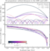 |
Fig. 5 Distances of possible S3 stream progenitors to the MW (top panel) and LMC (bottom panel; log scale) over the past 4 Gyr. The progenitors correspond to the streams shown in Fig. 4. The distances of progenitors initialised at 75 kpc (45 kpc) are shown as solid (dashed) lines. The colours indicate the progenitor’s Galactic standard of rest radial velocities (see the colour bar in the second row). All realisations orbit the MW, independent of chosen distances and radial velocities. Their closest approach to the LMC is ~100 Myr ago, when the progenitors of streams at closer distances get within 15 kpc of the LMC, and the farther progenitors between 15 and 50 kpc. |
5 Discussion
A considerable amount of effort has been devoted to understanding the impact of the LMC on the dynamics and morphology of MW stellar streams (e.g. Erkal et al. 2019; Koposov et al. 2019; Shipp et al. 2021; Vasiliev et al. 2021; Koposov et al. 2023; Lilleengen et al. 2023; Brooks et al. 2024). These studies have provided important insights into how the infall of the LMC perturbs the Galactic halo and influences the trajectories of MW substructures. In contrast, much less attention has been paid to stellar streams that are thought to be associated with the LMC, but whose membership remains largely tentative – such as the streams S1–S4 found by BK16 and later characterised by N19. Despite their potential to offer direct constraints on the LMC’s mass distribution, orbital history, and interaction with the MW, systematic efforts to identify and characterise potential LMC streams remain relatively scarce.
To address this gap, in this work, we first used Gaia DR3 proper motions to kinematically characterise and confirm the existence of the S3 stellar stream, which had previously been identified only through photometric data. Building on this, we applied a neural network classifier to search for new S3 candidate members, identifying 1542 stars. This represents a substantial increase over the ~10 stars previously known and provides a valuable foundation for future studies of the stream’s origin, properties, and possible association with the LMC. In Sect. 5.1 we place the S3 system in context by addressing its MW or LMC origin and outlining potential use-cases for its study, while in Sect. 5.2 we discuss possible follow-up observations aimed at confirming candidate members and further constraining the nature of the stream.
5.1 S3 in context: MW versus LMC stream and potential use-cases
We have explored a range of possible dynamical models for S3 in Sect. 4. These have revealed two results: (1) while the distance is ambiguous, S3 is likely at a large distance, and (2) all explored progenitor orbits are bound to the MW. The distance ambiguity stems from small number statistics and the uncertain classification of the 10 N19 stars into BHB and BS stars. The three clearly classified BS stars are at distances <50 kpc. If they were wrongly classified, and instead were BHB stars, we can assume a factor of two increase in their distance, putting them at distances between 80 and 100 kpc, more in line with the other stars.
While the progenitor orbits show a clear association with the MW, a possible association of the S3 stars with the LMC can be investigated by calculating their closest approach distance and velocity. If that velocity is larger than the LMC’s escape velocity at that distance, the star is unlikely to be associated with the LMC. We did this by backwards integrating the N19 stars in the MW–LMC simulation described in Sect. 4.1 and recording the closest approach. Figure 6 shows the distance and velocity relative to the LMC for the BHB (BS) stars marked as circles (squares). The magenta line shows the escape velocity curve for the LMC used in the simulation, a Hernquist sphere with MLMC = 1.25 × 10¹¹M⊙ and rs,LMC = 14.9 kpc. None of the stars are under the escape velocity line, which would indicate a clear association with the LMC. Some BS stars are at close distances and only slightly larger relative velocities; however, if they were reclassified as BHB stars, they would be at the distant end of the distribution (grey squares). This shows that the S3 stars are unlikely to be associated with the LMC.
While identifying S3 as an LMC stream would have opened up a new way of investigating the LMC’s present and past, S3 as an MW stream is interesting for both observers and theorists. S3 is remarkable for its combination of large Galactocentric distance and extended morphology. Two streams often used to model the halos of the MW and the LMC, and to understand their interaction, are the OC and the Sagittarius stream. While most of the OC stream is at a distance of ~20–30 kpc, its edges reach up to 60 kpc and are among its most informative parts (e.g. Erkal et al. 2019; Shipp et al. 2021; Lilleengen et al. 2023; Koposov et al. 2023). The Sagittarius stream reaches distances of close to 100 kpc, but most of the stream is within 60 kpc. It is notoriously difficult to model and needs the presence of the LMC (Vasiliev et al. 2021). We estimated the median distance of S3 to be ~75 kpc, and while Eridanus–M17 is the only known stream catalogued in galstreams (Mateu 2023) that surpasses S3 in distance (~95 kpc), it is extremely compact in projection compared to S3. Moreover, previous work by BK16 reported a stream width of 1.2°; with our expanded candidate sample, we find S3 to be nearly ~3–4° thick, indicating a substantial increase in its inferred physical width. Given the estimated median distance of S3 (~75 kpc), this angular width would translate to a physical thickness of roughly ~4–5 kpc, making S3 one of the thickest stellar streams discovered to date. Whether this thickness is driven by an interaction with the LMC or follows from properties of the progenitor is a question for future research.
These properties make S3 the most distant (~75 kpc) extended (~30° long, ~3–4° thick) stellar stream currently known in the MW, providing a unique opportunity to probe the outer Galactic halo and the recent dynamical influence of the LMC. Fitting the MW halo with the S3 stream will provide measurements at unprecedented distances that we have not gained from streams before, as streams are most informative in the distances they span (Bonaca & Hogg 2018). It will likely be informative on the LMC halo as well. Moreover, the MW–LMC interaction affects stellar streams. With its distance and extent, the S3 stream could become a very useful tracer of the halo deformations, which could ultimately help make predictions and constraints on the nature of dark matter (see the discussion in L23). However, to carry out these types of investigations, we need spectroscopic follow-up observations to build a detailed 6D picture of the S3 stream.
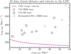 |
Fig. 6 Closest distance to the LMC and velocity at closest approach for the S3 BHB (BS) stars from N19, represented by white points (squares). The magenta line is the escape velocity curve of the LMC for a Hernquist sphere with MLMC = 1.25 × 10¹¹M⊙ and rs,LMC = 14.9 kpc. Any stars above the magenta line are likely not bound to the LMC. One BS has a close approach (~3 kpc) and a relatively low velocity with respect to the LMC (~330 km s−1). The other two BS stars are closer in distance and velocity to the LMC than most other BHB stars. However, if the BS stars were misclassified BHB stars (grey squares), they would be among the most distant stars with the highest velocity offsets. This suggests, independently of the stream models, that S3 is not of LMC origin. |
5.2 Follow-up observations
To advance our understanding of S3, spectroscopic follow-up of the newly identified candidates is essential. Line-of-sight velocity measurements will provide the missing sixth dimension of phase-space information, allowing us to reconstruct the stream’s orbit with far greater accuracy. Expanding coverage beyond the currently sparse and scattered measurements will help define the velocity profile, reduce contamination, constrain orbital parameters such as pericentre, apocentre, and angular momentum, and probe the stream’s internal kinematics as well as possible perturbations induced by the LMC.
Beyond kinematics, spectroscopy will also deliver independent distance estimates for RC stars, which make up roughly 30% of the new candidates identified in the catalogue of S3 candidates released alongside this work. These measurements, reliable even at 60–80 kpc, would sharpen the 3D map of the stream, refine its physical width and line-of-sight structure, and enable the detection of metallicity and age gradients. As a preliminary check on distances, we also crossmatched the sample with the Gaia DR3 RR Lyrae catalogue, but only a handful of stars overlapped, yielding too few matches to provide strong constraints (see Appendix D). Finally, spectroscopic abundances would provide a crucial chemical fingerprint of S3, helping distinguish between a dwarf galaxy or globular cluster progenitor, assess the presence of multiple stellar populations, and compare the stream’s properties with those of other halo substructures.
Together, these observations would anchor high-fidelity dynamical and chemical models of S3, enabling a detailed reconstruction of its orbital history, progenitor properties, and disruption timescale. They would also provide new constraints on the mass distribution of the outer MW and on the dynamical influence of the LMC.
6 Conclusions
Despite extensive study of the LMC’s influence on MW stellar streams, those directly associated with the LMC and SMC have received little attention. Only a few candidate stellar streams (S1–S4) beyond the Magellanic Stream have been reported. Identified before Gaia, these streams remain largely unexplored with modern astrometric data and current state-of-the-art modelling.
In this work we built upon these previous analyses, focusing on the S3 stream, a long (~30°) and narrow (~1.2°) stream at distances ranging from 60 to 80 kpc that points nearly exactly in the direction of the LMC. We pursued three primary objectives: (1) to extend the kinematic analysis of the S3 stellar candidates identified by N19 by incorporating astrometric data from Gaia DR3, with the goal of reassessing and validating the stream’s existence; (2) to expand the sample of potential S3 members using machine learning techniques; and (3) to generate stream models to determine S3’s association with either the MW or the LMC and to gain a better understanding of the data and future observation needs. Our main findings and conclusions are the following:
We report 1542 new high-confidence S3 stream candidates, greatly enlarging the previous sample of ~10 BHB and BS stars from N19;
Among these, we find 440 potential RC stars, which provide valuable targets for spectroscopic follow-up thanks to their well-defined luminosities and precise distance measurements.
Compared to earlier studies, S3’s apparent width has increased from ~1.2° to ~3–4°;
Through modelling and by comparing the closest-approach distance and velocity of S3 stars with the LMC’s escape velocity, S3 is identified as a distant stream (~75 kpc) linked to the MW that experienced a recent (~100 Myr) close encounter with the LMC;
Stream models are not yet particularly constraining of the precise orbit or the progenitor properties; future observations will help break degeneracies.
To sum up, we find that S3 is the most distant (~75 kpc) and extended (~30° long, ~3–4° thick) MW stream known, offering a unique window into the outer Galactic halo and the recent dynamical influence of the LMC. Its angular width corresponds to a physical thickness of ~4–5 kpc, making it one of the thickest stellar streams discovered to date. Fully exploiting the potential of S3 will require improved astrometric data; in particular, Gaia DR4, expected by the end of 2026, will provide proper motions that are at least twice as accurate as the current catalogue. Combined with spectroscopic follow-up from future surveys such as 4MOST (de Jong et al. 2019) or SDSS-V (Kollmeier et al. 2017, 2026), these data will enable a more precise characterisation of the stream’s kinematics and chemistry, confirmation of member stars, and a deeper understanding of its origin and dynamical history.
Data availability
The table containing the highly reliable S3 stream candidates is available at the CDS via https://cdsarc.cds.unistra.fr/viz-bin/cat/J/A+A/706/A253.
Acknowledgements
We thank the anonymous referee for a critical review and constructive suggestions that helped improving the manuscript. We thank Sergey Koposov for instructive conversations on the data. We are grateful to Marcel Bernet for his always valuable suggestions that improved the clarity and aesthetics of the figures. OJA acknowledges funding from “Swedish National Space Agency 2023-00154 David Hobbs The GaiaNIR Mission” and “Swedish National Space Agency 2023-00137 David Hobbs The Extended Gaia Mission”. MSP acknowledges support from a UKRI Stephen Hawking Fellowship. This work has made use of data from the European Space Agency (ESA) mission Gaia (https://www.cosmos.esa.int/gaia), processed by the Gaia Data Processing and Analysis Consortium (DPAC, https://www.cosmos.esa.int/web/gaia/dpac/consortium). Funding for the DPAC has been provided by national institutions, in particular the institutions participating in the Gaia Multilateral Agreement.
Software: ASTROPY (Astropy Collaboration 2013, 2018, 2022), CMASHER (van der Velden 2020), EXP (Petersen et al. 2022b; Petersen & Weinberg 2025), IPYTHON (Pérez & Granger 2007), JUPYTER (Kluyver et al. 2016), MATPLOTLIB (Hunter 2007), NUMPY (Harris et al. 2020), PANDAS (McKinney 2010; Reback et al. 2020), SCIPY (Virtanen et al. 2020), SHAP (Lundberg & Lee 2017), SKLEARN (Pedregosa et al. 2011).
References
- Arora, A., Garavito-Camargo, N., Sanderson, R. E., et al. 2024, ApJ, 974, 286 [Google Scholar]
- Astropy Collaboration (Robitaille, T. P., et al.) 2013, A&A, 558, A33 [NASA ADS] [CrossRef] [EDP Sciences] [Google Scholar]
- Astropy Collaboration (Price-Whelan, A. M., et al.) 2018, AJ, 156, 123 [Google Scholar]
- Astropy Collaboration (Price-Whelan, A. M., et al.) 2022, ApJ, 935, 167 [NASA ADS] [CrossRef] [Google Scholar]
- Bajaja, E., Cappa de Nicolau, C. E., Cersosimo, J. C., et al. 1985, ApJS, 58, 143 [Google Scholar]
- Belokurov, V., & Koposov, S. E. 2016, MNRAS, 456, 602 [NASA ADS] [CrossRef] [Google Scholar]
- Belokurov, V., Zucker, D. B., Evans, N. W., et al. 2006, ApJ, 642, L137 [Google Scholar]
- Besla, G., Kallivayalil, N., Hernquist, L., et al. 2012, MNRAS, 421, 2109 [Google Scholar]
- Bílek, M., Duc, P.-A., Cuillandre, J.-C., et al. 2020, MNRAS, 498, 2138 [Google Scholar]
- Binney, J. 2008, MNRAS, 386, L47 [Google Scholar]
- Bonaca, A., & Hogg, D. W. 2018, ApJ, 867, 101 [NASA ADS] [CrossRef] [Google Scholar]
- Bonaca, A., & Price-Whelan, A. M. 2025, New A Rev., 100, 101713 [Google Scholar]
- Borsato, N. W., Martell, S. L., & Simpson, J. D. 2020, MNRAS, 492, 1370 [NASA ADS] [CrossRef] [Google Scholar]
- Bovy, J., Bahmanyar, A., Fritz, T. K., & Kallivayalil, N. 2016, ApJ, 833, 31 [NASA ADS] [CrossRef] [Google Scholar]
- Brooks, R. A. N., Sanders, J. L., Lilleengen, S., Petersen, M. S., & Pontzen, A. 2024, MNRAS, 532, 2657 [Google Scholar]
- Brooks, R. A. N., Garavito-Camargo, N., Johnston, K. V., et al. 2025, ApJ, 978, 79 [Google Scholar]
- Brooks, R. A. N., Sanders, J. L., Dillamore, A. M., Garavito-Camargo, N., & Price-Whelan, A. M. 2026, MNRAS, 545, staf2111 [Google Scholar]
- Chandra, V., Naidu, R. P., Conroy, C., et al. 2023, ApJ, 956, 110 [CrossRef] [Google Scholar]
- Chandra, V., Naidu, R. P., Conroy, C., et al. 2025, ApJ, 988, 156 [Google Scholar]
- Clementini, G., Ripepi, V., Garofalo, A., et al. 2023, A&A, 674, A18 [NASA ADS] [CrossRef] [EDP Sciences] [Google Scholar]
- de Jong, R. S., Agertz, O., Berbel, A. A., et al. 2019, The Messenger, 175, 3 [NASA ADS] [Google Scholar]
- Dhanush, S. R., Subramaniam, A., & Subramanian, S. 2024, ApJ, 968, 103 [Google Scholar]
- Diehl, H. T., Abbott, T. M. C., Annis, J., et al. 2014, SPIE Conf. Ser., 9149, 91490V [Google Scholar]
- D’Onghia, E., & Fox, A. J. 2016, ARA&A, 54, 363 [Google Scholar]
- Dubinski, J., Mihos, J. C., & Hernquist, L. 1999, ApJ, 526, 607 [CrossRef] [Google Scholar]
- Erkal, D., Belokurov, V., Bovy, J., & Sanders, J. L. 2016, MNRAS, 463, 102 [NASA ADS] [CrossRef] [Google Scholar]
- Erkal, D., Belokurov, V., Laporte, C. F. P., et al. 2019, MNRAS, 487, 2685 [Google Scholar]
- Ferguson, P. S., Shipp, N., Drlica-Wagner, A., et al. 2022, AJ, 163, 18 [NASA ADS] [CrossRef] [Google Scholar]
- Gaia Collaboration (Prusti, T., et al.) 2016, A&A, 595, A1 [NASA ADS] [CrossRef] [EDP Sciences] [Google Scholar]
- Gaia Collaboration (Brown, A. G. A., et al.) 2018, A&A, 616, A1 [NASA ADS] [CrossRef] [EDP Sciences] [Google Scholar]
- Gaia Collaboration (Brown, A. G. A., et al.) 2021a, A&A, 649, A1 [NASA ADS] [CrossRef] [EDP Sciences] [Google Scholar]
- Gaia Collaboration (Luri, X., et al.) 2021b, A&A, 649, A7 [EDP Sciences] [Google Scholar]
- Gaia Collaboration (Vallenari, A., et al.) 2023, A&A, 674, A1 [NASA ADS] [CrossRef] [EDP Sciences] [Google Scholar]
- Garavito-Camargo, N., Besla, G., Laporte, C. F. P., et al. 2019, ApJ, 884, 51 [NASA ADS] [CrossRef] [Google Scholar]
- Garavito-Camargo, N., Besla, G., Laporte, C. F. P., et al. 2021, ApJ, 919, 109 [NASA ADS] [CrossRef] [Google Scholar]
- Gatto, M., Napolitano, N. R., Spiniello, C., Longo, G., & Paolillo, M. 2020, A&A, 644, A134 [NASA ADS] [CrossRef] [EDP Sciences] [Google Scholar]
- Gibbons, S. L. J., Belokurov, V., & Evans, N. W. 2014, MNRAS, 445, 3788 [NASA ADS] [CrossRef] [Google Scholar]
- Graczyk, D., Pietrzyński, G., Thompson, I. B., et al. 2014, ApJ, 780, 59 [Google Scholar]
- Grillmair, C. J., & Dionatos, O. 2006, ApJ, 643, L17 [Google Scholar]
- Harris, C. R., Millman, K. J., van der Walt, S. J., et al. 2020, Nature, 585, 357 [NASA ADS] [CrossRef] [Google Scholar]
- Hunter, J. D. 2007, Comput. Sci. Eng., 9, 90 [NASA ADS] [CrossRef] [Google Scholar]
- Ibata, R., Malhan, K., Tenachi, W., et al. 2024, ApJ, 967, 89 [NASA ADS] [CrossRef] [Google Scholar]
- Iorio, G., & Belokurov, V. 2021, MNRAS, 502, 5686 [Google Scholar]
- Ivezić, Ž., Kahn, S. M., Tyson, J. A., et al. 2019, ApJ, 873, 111 [Google Scholar]
- Jiménez-Arranz, Ó. & Roca-Fàbrega, S. 2025, A&A, 698, L7 [NASA ADS] [CrossRef] [EDP Sciences] [Google Scholar]
- Jiménez-Arranz, Ó., Romero-Gómez, M., Luri, X., & Masana, E. 2023a, A&A, 672, A65 [NASA ADS] [CrossRef] [EDP Sciences] [Google Scholar]
- Jiménez-Arranz, Ó., Romero-Gómez, M., Luri, X., et al. 2023b, A&A, 669, A91 [NASA ADS] [CrossRef] [EDP Sciences] [Google Scholar]
- Jiménez-Arranz, Ó., Chemin, L., Romero-Gómez, M., et al. 2024a, A&A, 683, A102 [NASA ADS] [CrossRef] [EDP Sciences] [Google Scholar]
- Jiménez-Arranz, Ó., Roca-Fàbrega, S., Romero-Gómez, M., et al. 2024b, A&A, 688, A51 [NASA ADS] [CrossRef] [EDP Sciences] [Google Scholar]
- Jiménez-Arranz, Ó., Horta, D., van der Marel, R. P., et al. 2025, A&A, 698, A88 [NASA ADS] [CrossRef] [EDP Sciences] [Google Scholar]
- Johnston, K. V., Majewski, S. R., Siegel, M. H., Reid, I. N., & Kunkel, W. E. 1999, AJ, 118, 1719 [NASA ADS] [CrossRef] [Google Scholar]
- Johnston, K. V., Law, D. R., & Majewski, S. R. 2005, ApJ, 619, 800 [Google Scholar]
- Kacharov, N., Tahmasebzadeh, B., Cioni, M.-R. L., et al. 2024, A&A, 692, A40 [NASA ADS] [CrossRef] [EDP Sciences] [Google Scholar]
- Kado-Fong, E., Greene, J. E., Hendel, D., et al. 2018, ApJ, 866, 103 [NASA ADS] [CrossRef] [Google Scholar]
- Kingma, D. P., & Ba, J. 2017, Adam: A Method for Stochastic Optimization [Google Scholar]
- Kluyver, T., Ragan-Kelley, B., Pérez, F., et al. 2016, in Positioning and Power in Academic Publishing: Players, Agents and Agendas, eds. F. Loizides, & B. Scmidt (Netherlands: IOS Press), 87 [Google Scholar]
- Kollmeier, J. A., Zasowski, G., Rix, H.-W., et al. 2017, arXiv e-prints [arXiv:1711.03234] [Google Scholar]
- Kollmeier, J. A., Rix, H.-W., Aerts, C., et al. 2026, AJ, 171, 52 [Google Scholar]
- Koposov, S. E., Rix, H.-W., & Hogg, D. W. 2010, ApJ, 712, 260 [Google Scholar]
- Koposov, S. E., Belokurov, V., Torrealba, G., & Evans, N. W. 2015, ApJ, 805, 130 [NASA ADS] [CrossRef] [Google Scholar]
- Koposov, S. E., Belokurov, V., Li, T. S., et al. 2019, MNRAS, 485, 4726 [Google Scholar]
- Koposov, S. E., Erkal, D., Li, T. S., et al. 2023, MNRAS, 521, 4936 [NASA ADS] [CrossRef] [Google Scholar]
- Law, D. R., & Majewski, S. R. 2010, ApJ, 714, 229 [Google Scholar]
- Lilleengen, S., Petersen, M. S., Erkal, D., et al. 2023, MNRAS, 518, 774 [Google Scholar]
- Lucchini, S., D’Onghia, E., Fox, A. J., et al. 2020, Nature, 585, 203 [CrossRef] [Google Scholar]
- Lucchini, S., D’Onghia, E., & Fox, A. J. 2021, ApJ, 921, L36 [NASA ADS] [CrossRef] [Google Scholar]
- Lundberg, S. M., & Lee, S.-I. 2017, in Advances in Neural Information Processing Systems, 30 (Curran Associates, Inc.) [Google Scholar]
- Malhan, K., & Ibata, R. A. 2018, MNRAS, 477, 4063 [Google Scholar]
- Martínez-Delgado, D., Gabany, R. J., Crawford, K., et al. 2010, AJ, 140, 962 [Google Scholar]
- Martínez-Delgado, D., Cooper, A. P., Román, J., et al. 2023, A&A, 671, A141 [NASA ADS] [CrossRef] [EDP Sciences] [Google Scholar]
- Martínez-Delgado, D., Stein, M., Sakowska, J. D., et al. 2025, A&A, 701, A182 [NASA ADS] [CrossRef] [EDP Sciences] [Google Scholar]
- Mateu, C. 2023, MNRAS, 520, 5225 [Google Scholar]
- McKinney, W. 2010, in Proceedings of the 9th Python in Science Conference, eds. S. van der Walt, & J. Millman, 56 [Google Scholar]
- Miró-Carretero, J., Martínez-Delgado, D., Gómez-Flechoso, M. A., et al. 2024, A&A, 691, A196 [NASA ADS] [CrossRef] [EDP Sciences] [Google Scholar]
- Navarrete, C., Belokurov, V., Catelan, M., et al. 2019, MNRAS, 483, 4160 [Google Scholar]
- Navarrete, C., Aguado, D. S., Belokurov, V., et al. 2023, MNRAS, 523, 4720 [Google Scholar]
- Necib, L., Ostdiek, B., Lisanti, M., et al. 2020, ApJ, 903, 25 [NASA ADS] [CrossRef] [Google Scholar]
- Newberg, H. J., Yanny, B., Rockosi, C., et al. 2002, ApJ, 569, 245 [Google Scholar]
- Nidever, D. L., Majewski, S. R., & Butler Burton, W. 2008, ApJ, 679, 432 [Google Scholar]
- Patrick, J. M., Koposov, S. E., & Walker, M. G. 2022, MNRAS, 514, 1757 [Google Scholar]
- Pearson, S., Clark, S. E., Demirjian, A. J., et al. 2022a, ApJ, 926, 166 [NASA ADS] [CrossRef] [Google Scholar]
- Pearson, S., Price-Whelan, A. M., Hogg, D. W., et al. 2022b, ApJ, 941, 19 [NASA ADS] [CrossRef] [Google Scholar]
- Pearson, S., Bonaca, A., Chen, Y., & Gnedin, O. Y. 2024, ApJ, 976, 54 [Google Scholar]
- Pedregosa, F., Varoquaux, G., Gramfort, A., et al. 2011, J. Mach. Learn. Res., 12, 2825 [Google Scholar]
- Pérez, F., & Granger, B. E. 2007, Comput. Sci. Eng., 9, 21 [Google Scholar]
- Petersen, M. S., & Peñarrubia, J. 2020, MNRAS, 494, L11 [NASA ADS] [CrossRef] [Google Scholar]
- Petersen, M. S., & Peñarrubia, J. 2021, Nat. Astron., 5, 251 [NASA ADS] [CrossRef] [Google Scholar]
- Petersen, M., & Weinberg, M. 2025, J. Open Source Softw., 10, 7302 [Google Scholar]
- Petersen, M. S., Peñarrubia, J., & Jones, E. 2022a, MNRAS, 514, 1266 [CrossRef] [Google Scholar]
- Petersen, M. S., Weinberg, M. D., & Katz, N. 2022b, MNRAS, 510, 6201 [NASA ADS] [CrossRef] [Google Scholar]
- Pettee, M., Thanvantri, S., Nachman, B., et al. 2024, MNRAS, 527, 8459 [Google Scholar]
- Pietrzyński, G., Graczyk, D., Gallenne, A., et al. 2019, Nature, 567, 200 [Google Scholar]
- Price-Whelan, A. M., & Bonaca, A. 2018, ApJ, 863, L20 [CrossRef] [Google Scholar]
- Price-Whelan, A. M., Hogg, D. W., Johnston, K. V., & Hendel, D. 2014, ApJ, 794, 4 [NASA ADS] [CrossRef] [Google Scholar]
- Putman, M. E. 2000, PASA, 17, 1 [Google Scholar]
- Putman, M. E., Staveley-Smith, L., Freeman, K. C., Gibson, B. K., & Barnes, D. G. 2003, ApJ, 586, 170 [NASA ADS] [CrossRef] [Google Scholar]
- Rathore, H., Choi, Y., Olsen, K. A. G., & Besla, G. 2025, ApJ, 978, 55 [Google Scholar]
- Reback, J., McKinney, W. jbrockmendel, et al. 2020, pandas-dev/pandas: Pandas 1.0.3 [Google Scholar]
- Rockosi, C. M., Odenkirchen, M., Grebel, E. K., et al. 2002, AJ, 124, 349 [NASA ADS] [CrossRef] [Google Scholar]
- Schölch, M., Jiménez-Arranz, Ó., Romero-Gómez, M., et al. 2025, A&A, 701, A227 [NASA ADS] [CrossRef] [EDP Sciences] [Google Scholar]
- Shih, D., Buckley, M. R., Necib, L., & Tamanas, J. 2022, MNRAS, 509, 5992 [Google Scholar]
- Shipp, N., Erkal, D., Drlica-Wagner, A., et al. 2021, ApJ, 923, 149 [NASA ADS] [CrossRef] [Google Scholar]
- Spergel, D., Gehrels, N., Baltay, C., et al. 2015, arXiv e-prints [arXiv:1503.03757] [Google Scholar]
- Springel, V., & White, S. D. M. 1999, MNRAS, 307, 162 [CrossRef] [Google Scholar]
- Starkman, N., Bovy, J., Webb, J. J., Calvetti, D., & Somersalo, E. 2023, MNRAS, 522, 5022 [Google Scholar]
- Tavangar, K., Ferguson, P., Shipp, N., et al. 2022, ApJ, 925, 118 [Google Scholar]
- Tavangar, K., & Price-Whelan, A. M. 2025, ApJ, 988, 45 [Google Scholar]
- The Dark Energy Survey Collaboration. 2005, [arXiv:astro-ph/0510346] [Google Scholar]
- van der Marel, R. P. 2001, AJ, 122, 1827 [Google Scholar]
- van der Velden, E. 2020, J. Open Source Softw., 5, 2004 [Google Scholar]
- Vasiliev, E. 2018, MNRAS, 481, L100 [Google Scholar]
- Vasiliev, E. 2024, MNRAS, 527, 437 [Google Scholar]
- Vasiliev, E., Belokurov, V., & Erkal, D. 2021, MNRAS, 501, 2279 [NASA ADS] [CrossRef] [Google Scholar]
- Virtanen, P., Gommers, R., Oliphant, T. E., et al. 2020, Nat. Methods, 17, 261 [Google Scholar]
- Weerasooriya, S., Starkenburg, T., Cunningham, E. C., & Johnston, K. V. 2025, arXiv e-prints [arXiv:2505.14792] [Google Scholar]
- Yaaqib, R., Petersen, M. S., & Peñarrubia, J. 2025, MNRAS, 544, 1820 [Google Scholar]
- Zaritsky, D., Chandra, V., Conroy, C., et al. 2025, Open J. Astrophys., 8, 16 [Google Scholar]
To compute the uncertainties in the orthographic proper motions (σvx, σvy), we applied Gaussian error propagation, taking into account both the individual uncertainties in (μα*, μδ) and their correlation. It calculates the partial derivatives of vx and vy with respect to μα* and μδ, and uses them – along with the covariance – to propagate the errors into the orthographic frame.
However, the catalogue of S3 stars released with this work includes the 2177 stars with P > 0.5 that also satisfy the polygon selection in proper motion space (see the end of Sect. 3.1 for further details). This allows other researchers interested in further studying the S3 stream to choose their own balance between completeness and purity based on their specific scientific goals.
These 440 RC candidate stars are identified in the catalogue of S3 candidates released alongside this work.
The mwlmc Python package, available at https://github.com/sophialilleengen/mwlmc, provides tools for accessing and working with the simulation data.
Appendix A S3 clean sample on-sky distribution for Pcut = 0.5
In this study we adopted a probability threshold of Pcut = 0.8 for the neural network classifier, prioritising a cleaner and less contaminated sample of S3 candidates, even at the expense of excluding some genuine members. Nevertheless, the main results presented in this work are robust across the probability threshold range of Pcut = 0.5 − 0.8. To illustrate this, Fig. A.1 presents the on-sky distribution of the S3 clean samples obtained with Pcut = 0.5, following the same format as Fig. 1. While the proper motion distribution of the neural network-selected sample (top panel) appears more irregular compared to the Pcut = 0.8 case (see Fig. 1), the application of the polygon selection (bottom panel) yields results broadly consistent with those discussed in the main text. To facilitate further studies of the S3 stream by other researchers – allowing them to adjust the balance between completeness and purity according to their specific goals – the released S3 star catalogue includes the 2177 stars with P > 0.5 that also meet the polygon selection criteria in proper motion space.
Appendix B Validation and explanation of the neural network classifier
To train and assess the performance of the classifier, we divided the sample of 10 200 stars (including both S3 and field stars) into two subsets: 60% for training the algorithm and 40% for testing its performance. We evaluated the classifier by generating the receiver ROC curve, the precision-recall curve, and calculating their respective AUCs. The ROC curve is a key metric for evaluating classification models, illustrating the trade-off between the true positive rate and false positive rate across different probability thresholds Pcut. Its AUC value reflects the model’s ability to distinguish between classes: the closer the AUC is to 1, the better the model performs. An AUC of 0.5 indicates no discriminative power. The precision-recall curve is particularly useful in scenarios with highly imbalanced classes, as in this case. Precision (the ratio of true positives to all stars classified as S3) indicates the relevance of the results, while recall (the ratio of true positives to all actual S3 stars) measures the completeness of the relevant results identified. Similar to the ROC curve, the precision-recall curve illustrates the trade-off between precision and recall across varying probability thresholds Pcut. The ROC curve, the precision-recall curve, and their corresponding AUC values all indicate an almost perfect classifier (see Fig. B.1). However, these results should be interpreted with caution, as they reflect performance on the subset of our simulated sample used for testing, rather than on the full Gaia DR3 dataset.
The SHAP summary plot shown in Fig. B.2 illustrates the impact of each input feature on the S3 classifier’s output, providing a detailed view of feature importance and the direction of their influence. Each point corresponds to an individual star from the test sample – consisting of 4080 stars, which make up 40% of the total 10 200 star training and testing dataset. The colour indicates the feature value (blue for low values, red for high), while the position along the x-axis shows the SHAP value, representing that feature’s contribution to the model’s classification output. Features are ranked by their overall importance (mean absolute SHAP value), with spatial position (x and y) and proper motion (vx and vy) emerging as the most influential variables. The spread of SHAP values along the x-axis for each feature indicates how much variation in model output is attributable to that feature. For instance, low values (blue) of vx tend to push the prediction towards one class (positive SHAP values), while high values (red) push it in the opposite direction. This analysis highlights which features are driving the classifier’s decisions and provides a level of interpretability often lacking in complex models.
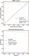 |
Fig. B.1 Evaluation metrics for the neural network classifier (see Sect. 3.1) performance. Top: ROC curve. Bottom: Precision-recall curve. In both cases, we compare our model (solid orange curve) with a classifier that has no class separation capacity (dashed purple curve). |
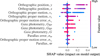 |
Fig. B.2 SHAP summary plot showing the impact of Gaia DR3 astrometric and photometric features on the S3 neural network model (see Sect. 3.1) output. Each dot represents an individual star from the test sample, which includes 4080 stars – accounting for 40% of the total dataset of 10 200 stars used for training and testing. Dot colour indicates the feature value (red for high, blue for low), while the position along the x-axis shows the SHAP value – that is, the feature’s contribution to the classification decision. Features are ordered from top to bottom by their overall importance, with those higher on the list having greater influence on the model’s output. |
Appendix C Stellar populations within the S3 new candidate sample
In Sect. 3.2 we analyse the different stellar populations within the S3 candidate sample using photometry. This is done by comparing the CMD of our sample with the LMC evolutionary phases defined in Gaia Collaboration (2021b), shifted to a distance of 73.5 kpc – the median distance of the N19 training sample – from the LMC mean distance of 49.5 kpc (Pietrzyński et al. 2019). Shifting the distance affects only the apparent magnitude in the CMD, as colour, being related to temperature and composition, remains unchanged. The shift is applied using the distance modulus:
![Mathematical equation: $\[m-M=5 ~\log _{10}(d / 10 ~\mathrm{pc}).\]$](/articles/aa/full_html/2026/02/aa57098-25/aa57098-25-eq1.png) (C.1)
(C.1)
The difference in apparent magnitude between the two distances is
![Mathematical equation: $\[\Delta m=5 ~\log _{10}\left(\frac{73.5 ~\mathrm{kpc}}{49.5 ~\mathrm{kpc}}\right)=0.86 ~\mathrm{mag} .\]$](/articles/aa/full_html/2026/02/aa57098-25/aa57098-25-eq2.png) (C.2)
(C.2)
Thus, the effect on the polygon selection is that the colour remains unchanged, while all apparent magnitudes in the CMD shift fainter by +0.86 mag, as the increased distance makes the stars appear dimmer. Figure C.1 shows the CMD of the S3 training sample from N19 (orange circles) and the 1542 new S3 candidates (beige circles), with the LMC CMD polygons from Gaia Collaboration (2021b) shifted to 73.5 kpc – the median distance of the N19 training sample. We find that the sample of 1542 new S3 stellar candidates is (as a first indication) predominantly composed of RC (29%) and RR Lyrae (25%) stars.
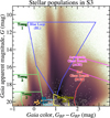 |
Fig. C.1 CMD showing the S3 training sample from N19 (orange circles) and the 1542 new S3 candidates (beige circles), with the LMC CMD polygons from Gaia Collaboration (2021b) shifted to 73.5 kpc – the median distance of the N19 training sample. The background image corresponds to the CMD of the Gaia DR3 sample utilised in this study (see Sect. 2.2). |
Appendix D RR Lyrae stars in the S3 new candidate sample
Given that the CMD polygon cut proposed by Gaia Collaboration (2021b) indicated the possible presence of RR Lyrae stars within our S3 clean sample, we attempted to crossmatch this sample with the Gaia DR3 RR Lyrae catalogue (gaiadr3.vari_rrlyrae; Clementini et al. 2023), aiming to identify any overlap between the datasets. However, we found only 3 (7) RR Lyrae stars at distances greater than 50 kpc within the neural network S3 sample after (before) applying the proper motion cut. The individual distances of those 3 RR Lyrae stars are 60, 55, and 73 kpc, placing some of them on the nearer side of the S3 stream. Figure D.1 displays the on-sky distribution of the RR Lyrae samples (pink circles), with arrows indicating their respective proper motions, in a similar manner to Fig. 1. The orientation and length of the arrows represent the direction and magnitude of the stars’ motion across the sky. This visualisation underscores both the spatial alignment and the coherent motion of the candidate members, illustrating that the stream is not only continuous in position but also coherent in proper motion space.
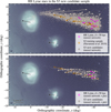 |
Fig. D.1 Same as Fig. 1 but highlighting in pink the 3 (7) RR Lyrae stars located beyond 50 kpc within the neural network S3 sample, after (before) applying the proper motion cut in the bottom (top) panel. |
All Figures
|
Fig. 1 Comparison of the on-sky distribution of the N19’s BHB–BS S3 training sample (orange circles) to the newly identified S3 candidates (beige circles), shown in the top panel using the neural network classifier alone, and in the bottom panel using both the neural network classifier and a polygon selection in proper motion space (see Sect. 3.1). The arrows’ orientation and length indicate the direction and magnitude of the stars’ motion across the sky, with a 2 mas yr−1 white arrow shown as a reference in the bottom panel. For the newly identified S3 candidates, we computed the median direction and magnitude of their motion across the sky within 1.6 × 1.6 deg2 bins, displaying the results only for bins containing more than 20 stars. The black arrows indicate the systemic motion of the LMC and SMC. The background image corresponds to a 2D histogram of the Gaia DR3 sample utilised in this study (see Sect. 2.2), consisting of 28 million stars that include both stars from the Clouds and foreground halo stars of the MW. Both panels are displayed using the orthographic projection (x, y, vx, vy) of the standard celestial coordinates (α, δ) and proper motions (μα*, μδ), centred in the LMC photometric centre, defined as (αc, δc) = (81.28°, −69.78°) by van der Marel (2001). |
| In the text | |
|
Fig. 2 Comparison of the proper motion distribution between the BHB–BS S3 training sample from N19 (orange circles) and the newly identified S3 candidates (beige and red transparent circles), overlaid on the Gaia DR3 sample (background histogram; see Sect. 2.2). The dashed black and white line indicates the polygon selection applied in proper motion space (see Sect. 3.1). The newly identified S3 candidates are shown in beige if they lie inside the polygon selection, and in transparent red if they fall outside it. The cyan and magenta crosses indicate the systemic motions of the LMC and SMC, respectively. In the background, regions of higher (lower) density are shown in bluer (redder) colour. |
| In the text | |
|
Fig. 3 Characterisation of the refined sample of 1542 new S3 stellar candidates (see Sect. 3.1). Top left panel: CMD of the S3 training sample by N19 (orange circles) and the new S3 candidates (beige circles). The background image corresponds to the CMD of the Gaia DR3 sample utilised in this study (see Sect. 2.2). Top centre and right panels: proper motion normalised distributions in right ascension (μα*) and declination (μδ), respectively. Bottom from left to right: parallax (ϖ) and proper motion error normalised distributions in right ascension (σμα*) and declination (σμδ). In the histograms, the S3 training sample from N19 is shown in orange and the new S3 candidates in beige. |
| In the text | |
|
Fig. 4 Observables of S3 BHB and BS data from N19 (white points and squares, respectively, with black error bars), neural network candidates (grey points and error bars), and the stream model (coloured points). The rows show the stream track, its heliocentric distance, radial velocity in the Galactic standard of rest, and proper motions, not reflex-corrected, respectively. The left (right) column shows model streams with a progenitor distance of 75 kpc (45 kpc). The colours refer to the progenitor’s Galactic standard of rest radial velocities (see the colour bar in the top-left panel). The streams at the larger distance (75 kpc) match the data well, particularly with a radial velocity of 50 km s−1. The closer progenitors (45 kpc) fail to produce streams that cover the whole range of all observables in ϕ1. |
| In the text | |
|
Fig. 5 Distances of possible S3 stream progenitors to the MW (top panel) and LMC (bottom panel; log scale) over the past 4 Gyr. The progenitors correspond to the streams shown in Fig. 4. The distances of progenitors initialised at 75 kpc (45 kpc) are shown as solid (dashed) lines. The colours indicate the progenitor’s Galactic standard of rest radial velocities (see the colour bar in the second row). All realisations orbit the MW, independent of chosen distances and radial velocities. Their closest approach to the LMC is ~100 Myr ago, when the progenitors of streams at closer distances get within 15 kpc of the LMC, and the farther progenitors between 15 and 50 kpc. |
| In the text | |
|
Fig. 6 Closest distance to the LMC and velocity at closest approach for the S3 BHB (BS) stars from N19, represented by white points (squares). The magenta line is the escape velocity curve of the LMC for a Hernquist sphere with MLMC = 1.25 × 10¹¹M⊙ and rs,LMC = 14.9 kpc. Any stars above the magenta line are likely not bound to the LMC. One BS has a close approach (~3 kpc) and a relatively low velocity with respect to the LMC (~330 km s−1). The other two BS stars are closer in distance and velocity to the LMC than most other BHB stars. However, if the BS stars were misclassified BHB stars (grey squares), they would be among the most distant stars with the highest velocity offsets. This suggests, independently of the stream models, that S3 is not of LMC origin. |
| In the text | |
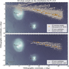 |
Fig. A.1 Same as Fig. 1 but for Pcut = 0.5. |
| In the text | |
|
Fig. B.1 Evaluation metrics for the neural network classifier (see Sect. 3.1) performance. Top: ROC curve. Bottom: Precision-recall curve. In both cases, we compare our model (solid orange curve) with a classifier that has no class separation capacity (dashed purple curve). |
| In the text | |
|
Fig. B.2 SHAP summary plot showing the impact of Gaia DR3 astrometric and photometric features on the S3 neural network model (see Sect. 3.1) output. Each dot represents an individual star from the test sample, which includes 4080 stars – accounting for 40% of the total dataset of 10 200 stars used for training and testing. Dot colour indicates the feature value (red for high, blue for low), while the position along the x-axis shows the SHAP value – that is, the feature’s contribution to the classification decision. Features are ordered from top to bottom by their overall importance, with those higher on the list having greater influence on the model’s output. |
| In the text | |
|
Fig. C.1 CMD showing the S3 training sample from N19 (orange circles) and the 1542 new S3 candidates (beige circles), with the LMC CMD polygons from Gaia Collaboration (2021b) shifted to 73.5 kpc – the median distance of the N19 training sample. The background image corresponds to the CMD of the Gaia DR3 sample utilised in this study (see Sect. 2.2). |
| In the text | |
|
Fig. D.1 Same as Fig. 1 but highlighting in pink the 3 (7) RR Lyrae stars located beyond 50 kpc within the neural network S3 sample, after (before) applying the proper motion cut in the bottom (top) panel. |
| In the text | |
Current usage metrics show cumulative count of Article Views (full-text article views including HTML views, PDF and ePub downloads, according to the available data) and Abstracts Views on Vision4Press platform.
Data correspond to usage on the plateform after 2015. The current usage metrics is available 48-96 hours after online publication and is updated daily on week days.
Initial download of the metrics may take a while.