| Issue |
A&A
Volume 706, February 2026
|
|
|---|---|---|
| Article Number | A75 | |
| Number of page(s) | 13 | |
| Section | Planets, planetary systems, and small bodies | |
| DOI | https://doi.org/10.1051/0004-6361/202557139 | |
| Published online | 03 February 2026 | |
TESS phase curve of ultra-hot Jupiter WASP-189 b★
1
Department of Astronomy, Stockholm University, AlbaNova University Center,
10691
Stockholm,
Sweden
2
Weltraumforschung und Planetologie, Physikalisches Institut, Universität Bern,
Gesellschaftsstrasse 6,
3012
Bern,
Switzerland
3
Center for Space and Habitability, Universität Bern,
Gesellschaftsstrasse 6,
3012
Bern,
Switzerland
4
Department of Physics, University of Warwick,
Gibbet Hill Road,
Coventry
CV4 7AL,
UK
5
Observatoire astronomique de l’Université de Genève,
Chemin Pegasi 51,
1290
Versoix,
Switzerland
6
INAF, Osservatorio Astrofisico di Catania,
Via S. Sofia 78,
95123
Catania,
Italy
★★ Corresponding author: This email address is being protected from spambots. You need JavaScript enabled to view it.
Received:
8
September
2025
Accepted:
3
December
2025
Abstract
Context. The thermal structures of highly irradiated ultra-hot Jupiters can deviate substantially from those of cooler hot Jupiters. For planets orbiting host stars that are rapidly rotating (and, thus, oblate), photometric light curves provide a unique opportunity to measure the spin-orbit angle. Moreover, in systems with significant spin-orbit misalignment, the stellar oblateness can induce an observable orbital precession.
Aims. We wish to study the atmosphere and orbital architecture of an ultra-hot Jupiter WASP-189 b, orbiting a hot A-type star.
Methods. We used the photometric phase curves and gravity-darkened transits of WASP-189 b observed with the Transiting Exoplanet Survey Satellite (TESS). We complemented these data with archival observations from CHaracterising ExOPlanet Satellite (CHEOPS).
Results. We detected a phase-curve signal with significant occultation depth of 203.4−16.3+16.2 ppm, while the nightside flux, −71.8−36.0+36.4 ppm, is consistent with zero at 2σ. We inverted the phase-curve signal to construct the temperature map of the planet. The map was subsequently used to estimate the Bond albedo and heat redistribution efficiency, whose expected median ranges were found to be 0.19–0.35 and 0.09–0.41, respectively. Finally, we analysed gravity-darkened transits to find that the planet is in polar orbit with the spin-orbit angle of 89.46−1.08+1.08 deg. We found no hint of any orbital precession when comparing our results with the literature.
Conclusions. Our observations, together with atmospheric modelling, suggest that the dayside emission of WASP-189b in TESS and CHEOPS bandpasses is dominated by thermal emission from an atmosphere with extremely inefficient heat transport and a negligible contribution from reflected light.
Key words: techniques: photometric / planets and satellites: atmospheres / planets and satellites: gaseous planets / planets and satellites: individual: WASP-189 b
The raw and detrended photometric data from TESS, along with codes to generate figures, can be found at: https://github.com/Jayshil/w189Figs
© The Authors 2026
 Open Access article, published by EDP Sciences, under the terms of the Creative Commons Attribution License (https://creativecommons.org/licenses/by/4.0), which permits unrestricted use, distribution, and reproduction in any medium, provided the original work is properly cited.
This article is published in open access under the Subscribe to Open model. This email address is being protected from spambots. You need JavaScript enabled to view it. to support open access publication.
1 Introduction
The population of hot Jupiters with extremely high temperatures (Teq ≳ 2200 K) has emerged as a distinct class of planets, known as ultra-hot Jupiters. They have dissimilar atmospheric properties compared to the cooler hot Jupiters. In particular, while the cooler hot Jupiters have absorption features in their occultation depth spectra (e.g. Stevenson et al. 2014), the ultra-hot Jupiters’ spectra are either featureless blackbody-like or have emission features (e.g. Sheppard et al. 2017; Mansfield et al. 2018; Coulombe et al. 2023). The change from absorption to emission features is a result of changing the temperature profile from non-inverted to inverted. Mansfield et al. (2021) revealed the trend of spectral features in occultation depth spectra of hot Jupiters, namely, that the spectral features change from absorption to emission and eventually become muted with increasing equilibrium temperature. The emergence of short-wave absorbers, such as TiO and VO, in the upper atmosphere at higher temperatures (≳2000 K), creates an inverted temperature profile that results in emission features in the spectra (e.g. Mansfield et al. 2021). At even higher temperatures (≳3000 K), while the temperature profile is still inverted, the molecular dissociation and the presence of H− continuum opacity mute the spectral features (e.g. Arcangeli et al. 2018; Parmentier et al. 2018; Mansfield et al. 2021). The H− opacity also causes a low dayside geometric albedo of the planet.
Hot Jupiters have a strong day-night temperature difference (see e.g. Heng & Showman 2015, for a review). The temperature contrast is expected to increase with temperature because the radiative cooling becomes more efficient compared to the efficiency of the heat transport to the nightside of the planet (e.g. Komacek & Showman 2016). However, this trend might break for ultra-hot Jupiters: the dissociated molecular H2, which forms atomic H on the dayside, because of high temperatures, would recombine to again create H2 on the nightside. This can increase the day–night energy transport and thus effectively reduce the day-night temperature contrast (Bell & Cowan 2018). Phase curve observations of several ultra-hot Jupiters, such as KELT-9 b, are already showing hints of this in terms of smaller (albeit not reaching zero) heat redistribution efficiency (e.g. Mansfield et al. 2020; Jones et al. 2022).
WASP-189 b, an ultra-hot Jupiter around a hot, fast-rotating A-type star (Anderson et al. 2018) with an equilibrium temperature of ![Mathematical equation: $\[3353_{-34}^{+27}\]$](/articles/aa/full_html/2026/02/aa57139-25/aa57139-25-eq4.png) K (Lendl et al. 2020), is one of the prime targets to study the dayside emission and thermal structure of ultra-hot Jupiters. Its high-resolution observations in transmission have successfully detected several species including TiO, V, Fe, Fe+, Ti, Ti+, Cr, Mg, Mg+, Mn, H, Na, Ca, Ca+, Ni, Sr, Sr+, and Ba+ (Prinoth et al. 2022, 2023; Sreejith et al. 2023; Prinoth et al. 2024). At the same time, the high-resolution dayside emission spectroscopy from the ground further identified CO, Fe (Yan et al. 2022; Deibert et al. 2024; Lesjak et al. 2025). The presence of short-wave absorbers, such as TiO, results in an inverted temperature profile (Yan et al. 2022; Lesjak et al. 2025), which is previously seen for other ultra-hot Jupiters (Mansfield et al. 2021). The non-detection of Fe in near-infrared high-resolution transmission spectroscopy by Vaulato et al. (2025) was thought to be because of the presence of H−. CHaracterising ExOPlanet Satellite (CHEOPS; Benz et al. 2021) has observed several occultations and phase curves of WASP-189b with its optical bandpass (Lendl et al. 2020; Deline et al. 2022). They detected a significant occultation depth in the optical bandpass of CHEOPS, which they suggested could be explained solely by thermal emission from the planet in the case of extremely inefficient heat redistribution. Deline et al. (2022) suggested that the reflective light might contribute to the occultation depth observed in the CHEOPS bandpass and places an upper limit of 0.48 on the geometric albedo. The ultra-precise transit observations with CHEOPS further showed gravity darkening that subsequently led Lendl et al. (2020); Deline et al. (2022) to determine its orbital architecture. The planet was found to be in a polar orbit around its host star.
K (Lendl et al. 2020), is one of the prime targets to study the dayside emission and thermal structure of ultra-hot Jupiters. Its high-resolution observations in transmission have successfully detected several species including TiO, V, Fe, Fe+, Ti, Ti+, Cr, Mg, Mg+, Mn, H, Na, Ca, Ca+, Ni, Sr, Sr+, and Ba+ (Prinoth et al. 2022, 2023; Sreejith et al. 2023; Prinoth et al. 2024). At the same time, the high-resolution dayside emission spectroscopy from the ground further identified CO, Fe (Yan et al. 2022; Deibert et al. 2024; Lesjak et al. 2025). The presence of short-wave absorbers, such as TiO, results in an inverted temperature profile (Yan et al. 2022; Lesjak et al. 2025), which is previously seen for other ultra-hot Jupiters (Mansfield et al. 2021). The non-detection of Fe in near-infrared high-resolution transmission spectroscopy by Vaulato et al. (2025) was thought to be because of the presence of H−. CHaracterising ExOPlanet Satellite (CHEOPS; Benz et al. 2021) has observed several occultations and phase curves of WASP-189b with its optical bandpass (Lendl et al. 2020; Deline et al. 2022). They detected a significant occultation depth in the optical bandpass of CHEOPS, which they suggested could be explained solely by thermal emission from the planet in the case of extremely inefficient heat redistribution. Deline et al. (2022) suggested that the reflective light might contribute to the occultation depth observed in the CHEOPS bandpass and places an upper limit of 0.48 on the geometric albedo. The ultra-precise transit observations with CHEOPS further showed gravity darkening that subsequently led Lendl et al. (2020); Deline et al. (2022) to determine its orbital architecture. The planet was found to be in a polar orbit around its host star.
It is difficult to constrain the reflective properties of the dayside with only one CHEOPS photometric occultation depth. Here, we present another photometric observation of WASP-189 b taken with the Transiting Exoplanet Survey Satellite (TESS; Ricker et al. 2014). While CHEOPS and TESS bandpasses overlap for a range of wavelengths, the TESS bandpass is more sensitive to longer wavelengths. In the absence of other spectroscopic observations of WASP-189b, combined TESS and CHEOPS observations can constrain the thermal properties of the planetary atmosphere, which is the prime goal of the present work. Furthermore, since the TESS observations were obtained almost two years after the CHEOPS observations, we also searched for the orbital precession, which can occur for planets in misaligned orbits around fast-rotating oblate stars. Section 2 describes our manual data reduction procedure to extract photometry from the TESS target pixel files (TPFs) and details the planetary, stellar, and instrumental models that we used to fit the data. Section 3 presents the results and discusses their meaning for the planet and its atmosphere. Finally, we discuss stellar variability in Sect. 4, followed by our conclusion in Sect. 5.
2 Observations and data analysis
2.1 Observations and data reduction
WASP-189 was observed with TESS during its extended mission in Sector 51. The raw data were reduced by the TESS Science Processing Operation Center (SPOC; Jenkins et al. 2016) to produce PDC-SAP photometry (Presearch Data Conditioning Simple Aperture Photometry; Smith et al. 2012; Stumpe et al. 2014). The PDC-SAP light curve, shown in Fig. B.1, has large gaps in it. In the hope of recovering some of the data, we decided to use our own data reduction pipeline to reduce TESS photometry from TPFs. We first computed a simple aperture photometry by summing up all counts inside the aperture, where the aperture is defined by selecting 15 brightest pixels in the median 2D TPF. We subtract the median of the background flux from all pixels inside the aperture before calculating the photometry. We removed all points with NaN values and 20σ outliers. The resultant photometry, shown in Fig. B.1, is heavily affected by the instrumental systematics. We employed the pixel-level decorrelation technique that performs principal component analysis (PCA) on pixel-level light curves of all pixels within the aperture to model instrumental systematics. The first few principal components (PCs) should trace the instrumental systematics. To select how many PCs to include in our model, we performed a linear detrending of simple aperture photometry with a model generated from a set of PCs. We added the PCs to the model one-by-one and kept the PCs that produced a detrended photometry with the lowest median absolute deviation (MAD). We found that the use of the first four PCs minimised the MAD, which we eventually used as linear decorrelation vectors in our light curve analysis to model the instrumental systematics (see Sect. 2.4). We masked all the points with a high background larger than 100 e−/s. This technique was previously used to model the instrumental systematics of Spitzer (Deming et al. 2015), K2 (Luger et al. 2016), and the James Webb Space Telescope (JWST; Patel et al. 2024).
2.2 Gravity darkened transit
The host star WASP-189 is a hot (Teff = 8000 ± 80 K), A-type star (Lendl et al. 2020). As with the other such hot stars, WASP-189 is a rapid rotator with v sin i = 93.1 ± 1.7 km/s (Lendl et al. 2020). A centrifugal force generated by the rapid stellar rotation distorts the shape of the star to make it oblate: the stellar equatorial radius will increase compared to its radius at the pole. von Zeipel (1924) showed that the local surface gravity, and thus the local temperature and resulting brightness, will change as a function of latitude on an oblate star: the stellar equator would appear darker compared to the poles, a phenomenon called gravity darkening. If a planet in a misaligned orbit were to transit a gravity-darkened oblate star, it would block the stellar disk of non-uniform brightness during its passage. This would lead to a peculiar asymmetric transit shape that is dependent on the exact geometry of the orbit and stellar orientation (Barnes 2009). It is therefore possible to extract information regarding the orbital geometry just from observing the transit. Indeed, gravity darkening induced asymmetric transit was observed previously for several planets, which constrained stellar and orbital orientation relative to the observer (Hooton et al. 2022; Jones et al. 2022).
Lendl et al. (2020) and Deline et al. (2022) already observed the gravity darkened transit of WASP-189 b using ultra-high precision photometry from CHEOPS. Following their results, we decided to fit a gravity-darkened transit model to the TESS data. We used the open-source Python package PyTransit (Parviainen 2015) to do this1. PyTransit first generates a discrete cell grid on the stellar surface and calculates the local surface gravity on these cells by assuming a star whose outer layers are deformed due to rapid rotation. PyTransit then uses von Zeipel’s theorem (von Zeipel 1924) to compute the surface temperature at each discrete cell on the stellar surface. A PHOENIX synthetic stellar spectrum (Husser et al. 2013), the TESS instrument response function, and the quadratic limb darkening law were used to compute the flux emitted from each discrete cell. PyTransit finally uses orbital parameters to estimate the light blocked by the planet during transit.
The gravity darkened transit model in PyTransit is parametrised by the planet-to-star radius ratio (Rp/R⋆), stellar density (ρ⋆), stellar rotation period (P⋆), and stellar obliquity with respect to the plane of the sky (ϕ⋆ = π/2 − i⋆, where i⋆ is the stellar inclination), gravity darkening parameter (β), limb darkening coefficients (u1 and u2 for the quadratic law), transit time (t0), planetary orbital period (P), scaled semi-major axis (a/R⋆), orbital inclination (ip), projected orbital obliquity (λp), eccentricity (e), and the argument of periastron passage (ω). We directly fit for all these parameters, except ρ⋆, P⋆, (u1, u2), and ip. We computed P⋆ from ϕ⋆, projected rotation speed (v sin i⋆), and radius (R⋆), which we treated as free parameters in our analysis, expressed as
![Mathematical equation: $\[P_{\star}=\frac{2 \pi R_{\star}}{v \sin i_{\star}} \sin i_{\star}=\frac{2 \pi R_{\star}}{v \sin i_{\star}} \sin \left(\pi / 2-\phi_{\star}\right).\]$](/articles/aa/full_html/2026/02/aa57139-25/aa57139-25-eq5.png) (1)
(1)
Furthermore, we can estimate the density of an oblate star using stellar oblateness (f⋆ = 1 − Rpole/R⋆, where Rpole is the pole radius), stellar mass, and rotation period (e.g. Deline et al. 2022),
![Mathematical equation: $\[f_{\star}=\frac{1}{1+\frac{G M_{\star} P_{\star}^2}{2 \pi^2 R_{\star}^3}}=\frac{3 \pi}{2 G \rho_{\star} P_{\star}^2}.\]$](/articles/aa/full_html/2026/02/aa57139-25/aa57139-25-eq6.png) (2)
(2)
The second equality in above equation is obtained by using the definition of stellar density for an oblate star,
![Mathematical equation: $\[\rho_{\star}=\frac{M_{\star}}{\frac{4}{3} \pi \cdot\left(R_{\text {equator }} \cdot R_{\text {equator }} \cdot R_{\text {pole }}\right)}=\frac{M_{\star}}{\frac{4}{3} \pi R_{\star}^3\left(1-f_{\star}\right)},\]$](/articles/aa/full_html/2026/02/aa57139-25/aa57139-25-eq7.png) (3)
(3)
in the second term of Eq. (2). Here, Requatoris the stellar radius at the equator, which we take as R⋆, and Rpole = R⋆(1 − f⋆).
We directly fit for M⋆ to obtain the stellar density from P⋆ and R⋆, using Eqs. (1) and (2). Then, ip and i⋆ are computed from b (impact parameter) and ϕ⋆, respectively. Instead of directly fitting for quadratic limb-darkening coefficients (u1 and u2), we used Kipping (2013) parametrisation to fit for limb darkening coefficients. Finally, we fit for b in our analysis instead of fitting for ip.
Many of the planetary orbital parameters used by PyTransit to generate the gravity-darkened transit model are highly correlated. Fitting for all of them without any prior knowledge can result in degeneracies among model parameters (e.g. Hooton et al. 2022). It is generally recommended to put informative priors on at least some of these parameters based on either Doppler tomography or other previous observations (Masuda 2015; Hooton et al. 2022). Deline et al. (2022) recently used CHEOPS transit observations to constrain planetary and stellar parameters for the WASP-189 system. Considering this point and given that the photometric precision of our five transits is lower than that of CHEOPS, we decided to put informative priors on most of the planetary and stellar parameters based on the analysis by Deline et al. (2022). A notable exception to this is the limb darkening coefficients, which could be wavelength-dependent. Thus, we decided to put uninformative priors on their Kipping (2013) parametrisation (see e.g. Patel & Espinoza 2022). The full list of parameters and priors used on them is provided in Table A.1. Since we use normal priors based on previous CHEOPS observations, our derived parameters will be an update on their literature values, without the need for simultaneous analyses of CHEOPS and TESS data.
2.3 Occultation and orbital phase curve
As demonstrated by Deline et al. (2022), the shape of the occultation light curve for an oblate star would be slightly different from that for a spherical star. Following their method, we set limb-darkening and gravity darkening coefficients in the PyTransit gravity darkened transit model to zero to obtain the occultation light curve. In doing so, we also set the “transit” time to the occultation time, ![Mathematical equation: $\[\lambda_{p}^{\prime}=-\lambda_{p}\]$](/articles/aa/full_html/2026/02/aa57139-25/aa57139-25-eq8.png) , and ω′ = ω + π. In the end, we normalise the occultation signal such that the flux inside the occultation is set to zero and the out-of-occultation flux is one. Normalisation was done so that we can directly multiply our phase curve model with the normalised occultation model to obtain flux variations due to the planet.
, and ω′ = ω + π. In the end, we normalise the occultation signal such that the flux inside the occultation is set to zero and the out-of-occultation flux is one. Normalisation was done so that we can directly multiply our phase curve model with the normalised occultation model to obtain flux variations due to the planet.
We modelled the out-of-transit and occultation variation using the implementation of Cowan & Agol (2008) phase curve model by Kempton et al. (2023) in our analysis, which is defined as
![Mathematical equation: $\[\begin{aligned}F_p= & E+C_1\left(\cos~ \omega_p t_e-1\right)+D_1 ~\sin~ \omega_p t_e \\& +C_2\left(\cos~ 2 \omega_p t_e-1\right)+D_2 ~\sin~ 2 \omega_p t_e.\end{aligned}\]$](/articles/aa/full_html/2026/02/aa57139-25/aa57139-25-eq9.png) (4)
(4)
Here, E, C1, D1, D2, and D2 are phase curve coefficients, te is the time since mid-occultation and ωp = 2π/P. Equation (4) is defined such that the parameter E gives the occultation depth. Being a simple sinusoidal function, this function is fast to evaluate. We note here that the above phase curve model only contains the planetary model. We do not model the ellipsoidal variations and the Doppler beaming since their amplitudes are expected to be very small (on the order of 10 and 1 ppm, respectively; Deline et al. 2022). It is possible to invert the Cowan & Agol (2008) phase curve function to obtain the temperature map of the planet.
We fit both the first-order (i.e. setting C2 = D2 = 0 in Eq. (4)) and second-order (non-zero C2 and D2) phase curve models to the data and compared the Bayesian evidence. Upon finding that the first-order model was heavily favoured compared to the second-order model, we fixed C2 and D2 to zero in our final analysis. We put wide, uninformative priors on phase curve parameters in our data analysis (see Table A.1).
2.4 Light travel time delay, noise sources, and posterior sampling
The light signal from the planet and the star does not reach the observer simultaneously because of the finite light travel time. We implemented a correction of the light travel time in our analysis, assuming a circular orbit and following the method from Deline et al. (2022), expressed as
![Mathematical equation: $\[t_{\mathrm{ref}}=t_{\mathrm{obs}}-\frac{a}{c}\left[1-\cos \left(2 \pi \frac{t_{\mathrm{obs}}-t_0}{P}\right)\right] \sin~ i_p.\]$](/articles/aa/full_html/2026/02/aa57139-25/aa57139-25-eq10.png) (5)
(5)
Here, a is the semi-major axis and c is the speed of light. We essentially computed our planetary and stellar models at tref for observed tobs while simultaneously fitting for a, t0, P, and ip.
The simple aperture photometry has strong instrumental systematics as described in Sect. 2.1. We included a linear model in the first four PCs from our PCA to model the instrumental systematics. We also tested if our results are sensitive to the number of PCs used in the analysis. While transit parameters are insensitive to the number of PCs, phase curve parameters can change if we include only one or two PCs, as very few PCs cannot model the instrumental systematics properly. This also results in large uncertainties on phase curve parameters. However, after inclusion of the third and more PCs, the values of phase curve parameters stabilise to the values we report here. While the detrending using PCs should take care of most of the instrumental noise, we found an additional noise source that could be astrophysical or leftover instrumental noise (see Sect. 4 for more details). We fit this noise with the help of a Gaussian process (GP) model based on the simple harmonic oscillator (SHO) kernel, as implemented in celerite2 (Foreman-Mackey et al. 2017; Foreman-Mackey 2018).
We used nested sampling methods (Skilling 2004, 2006), in particular, dynamic nested sampling (Higson et al. 2019) implemented in the dynesty (Speagle 2020) package to draw samples from the posterior distribution. The median and 16–84th percentile confidence intervals for our fitted parameters are given in Table A.1.
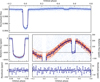 |
Fig. 1 Detrended and phase-folded TESS data along with the best-fit model. The light and dark blue points show the unbinned and binned data points. The dark blue and orange lines are the median model and models computed from randomly selected posteriors, respectively. Top: full phase curve with a transit and occultation. Middle: zoom-in on the transit (middle left) and occultation/phase curve (middle right). The dashed line represents the level of stellar flux (i.e. flux level during the occultation). The gravity darkened asymmetric transit and a phase variation, along with an occultation, are clearly visible in the middle panel. Bottom: residuals after subtracting the median model from the raw data. |
3 Results and discussion
3.1 Planetary orbit and orbital precession
Our results from the gravity-darkened transit analysis, shown in Table A.1, corroborate the results from Deline et al. (2022), which is expected given our choices of priors. Our prior choice also implies that the values for all planetary and stellar parameters (except for parameters specific to TESS; e.g. limb darkening coefficients and phase curve parameters) that we derived are updated from previous analyses. The best-fit gravity-darkened transit model, along with the data, is shown in Fig. 1. Using our best-fit planetary parameters, we constrained the 3D spin-orbit angle (Hooton et al. 2022; Deline et al. 2022),
![Mathematical equation: $\[\Psi=\arccos \left(\cos~ i_{\star} ~\cos~ i_p+\sin~ i_{\star} ~\sin~ i_p ~\cos~ \lambda_p\right),\]$](/articles/aa/full_html/2026/02/aa57139-25/aa57139-25-eq11.png) (6)
(6)
which defines the 3D angle between the stellar spin axis and the planetary orbital axis. We constrained its value to ![Mathematical equation: $\[89.46_{-1.08}^{+1.08}\]$](/articles/aa/full_html/2026/02/aa57139-25/aa57139-25-eq12.png) deg, suggesting a polar orbit. This value of Ψ is consistent with the literature values from Lendl et al. (2020) and Deline et al. (2022). Apart from Ψ, although we have properly constrained system parameters, there remains a degeneracy among the system parameters i⋆, ip, and λp inherent to a gravity darkening transit model. The issue is that it is not possible to distinguish between (i⋆, ip, λp) and (180° − i⋆, 180° − ip, − λp).
deg, suggesting a polar orbit. This value of Ψ is consistent with the literature values from Lendl et al. (2020) and Deline et al. (2022). Apart from Ψ, although we have properly constrained system parameters, there remains a degeneracy among the system parameters i⋆, ip, and λp inherent to a gravity darkening transit model. The issue is that it is not possible to distinguish between (i⋆, ip, λp) and (180° − i⋆, 180° − ip, − λp).
The polar orbit of WASP-189b and the stellar oblateness provide good conditions for planetary orbital precession. The stellar quadruple moment, J2, can perturb the orbit and cause precession (Masuda 2015). The precession can be detected as a temporal evolution of b (or, ip) and λp (Hooton et al. 2022). If detected, this would provide good constraints on J2. We performed another analysis of TESS data alone to see if there is any change in b and λp, compared to the CHEOPS results (Deline et al. 2022).
Deline et al. (2022) observed two high-precision phase curves of WASP-189b that contain three and a half transits. The TESS observations of WASP-189 occurred about two years after the first Deline et al. (2022) CHEOPS observations. This long baseline provides a unique opportunity to check if the orbit of WASP-189 b is precessing. Our main analysis of TESS data, described in Sect. 2, is highly influenced by the priors since we provided normal priors on b and λ. Therefore, we reanalysed the dataset in the same manner as described in Sect. 2. However, this time, we put uniform priors 𝒰(0.35, 0.50) and 𝒰(86, 97) on b and λp, respectively (here, 𝒰(a, b), represents uniform priors between a and b). We get b = ![Mathematical equation: $\[0.432_{-0.018}^{+0.016}\]$](/articles/aa/full_html/2026/02/aa57139-25/aa57139-25-eq13.png) and λp =
and λp = ![Mathematical equation: $\[89.88_{-2.70}^{+3.85}\]$](/articles/aa/full_html/2026/02/aa57139-25/aa57139-25-eq14.png) deg, which are within 1σ of their corresponding values from Deline et al. (2022), b = 0.433 ± 0.020 and λp = 91.7 ± 1.2 deg. The rate of change of b and λp, measured for the first time for WASP-189 b, are
deg, which are within 1σ of their corresponding values from Deline et al. (2022), b = 0.433 ± 0.020 and λp = 91.7 ± 1.2 deg. The rate of change of b and λp, measured for the first time for WASP-189 b, are ![Mathematical equation: $\[-1.59_{-39.35}^{+38.77}\]$](/articles/aa/full_html/2026/02/aa57139-25/aa57139-25-eq15.png) × 10−6 yr−1 and
× 10−6 yr−1 and ![Mathematical equation: $\[-0.0026_{-0.0043}^{+0.0058}\]$](/articles/aa/full_html/2026/02/aa57139-25/aa57139-25-eq16.png) deg yr−1, respectively, both of which are consistent with zero at 1σ. This means that we do not detect any significant orbital precession. However, this is not surprising given that the measured rate of change of b for other hot Jupiters is on the order of 0.01 yr−1 (e.g. Szabó et al. 2012; Johnson et al. 2015; Stephan et al. 2022; Watanabe et al. 2024). The rate of change of b is directly proportional to J2 (Watanabe et al. 2022). The exact value of J2 depends on the star: it was measured to be on the order of 10−4–10−5 for the early to late A-type stars KELT-9 and TOI-1518 (Stephan et al. 2022; Watanabe et al. 2024), so we should expect a similar value of J2 for WASP-189, which is also an A-type star. Therefore, we should expect a similar rate of change of b for WASP-189b. However, the rate is also directly proportional to cos Ψ and inversely proportional to a/R⋆ and P (Watanabe et al. 2022). WASP-189b has slightly larger values of a/R⋆ and P compared to KELT-9 b and TOI-1518 b, with Ψ ≈ 90°, thereby decreasing cos Ψ. This can decrease the rate of change of b to less than 0.01 yr−1. Our current observations do not significantly constrain such a small change. Observations over a long baseline might help in detecting orbital precession.
deg yr−1, respectively, both of which are consistent with zero at 1σ. This means that we do not detect any significant orbital precession. However, this is not surprising given that the measured rate of change of b for other hot Jupiters is on the order of 0.01 yr−1 (e.g. Szabó et al. 2012; Johnson et al. 2015; Stephan et al. 2022; Watanabe et al. 2024). The rate of change of b is directly proportional to J2 (Watanabe et al. 2022). The exact value of J2 depends on the star: it was measured to be on the order of 10−4–10−5 for the early to late A-type stars KELT-9 and TOI-1518 (Stephan et al. 2022; Watanabe et al. 2024), so we should expect a similar value of J2 for WASP-189, which is also an A-type star. Therefore, we should expect a similar rate of change of b for WASP-189b. However, the rate is also directly proportional to cos Ψ and inversely proportional to a/R⋆ and P (Watanabe et al. 2022). WASP-189b has slightly larger values of a/R⋆ and P compared to KELT-9 b and TOI-1518 b, with Ψ ≈ 90°, thereby decreasing cos Ψ. This can decrease the rate of change of b to less than 0.01 yr−1. Our current observations do not significantly constrain such a small change. Observations over a long baseline might help in detecting orbital precession.
3.2 Atmospheric properties
We detected a significant phase-curve signal in our TESS dataset, which we modelled using a Cowan & Agol (2008) phase curve model (see Fig. 1 for the data and the fitted phase curve model). Parametrisation of this model (Eq. (4)) allows us to estimate occultation depth and nightside flux as flux at the time of occultation (i.e. te = 0) and transit (te = P/2), respectively. According to this formulation, the occultation depth and nightside flux would be E and E − 2C1, respectively, which we compute to be ![Mathematical equation: $\[203.4_{-16.3}^{+16.2}\]$](/articles/aa/full_html/2026/02/aa57139-25/aa57139-25-eq17.png) ppm and
ppm and ![Mathematical equation: $\[-71.8_{-36.0}^{+36.4}\]$](/articles/aa/full_html/2026/02/aa57139-25/aa57139-25-eq18.png) ppm. While we constrain the occultation depth at more than 10σ, the nightside flux is consistent with zero at 2σ. The negative value of the nightside flux, which is consistent with zero at 2σ, is likely because of random chance, but it might be because of instrumental noise or uncorrected ellipsoidal variations (e.g. Deline et al. 2025). However, we note that the ellipsoidal variation is expected to be small for the WASP-189 system (see Sect.2.3). We find that the phase offset is consistent with zero,
ppm. While we constrain the occultation depth at more than 10σ, the nightside flux is consistent with zero at 2σ. The negative value of the nightside flux, which is consistent with zero at 2σ, is likely because of random chance, but it might be because of instrumental noise or uncorrected ellipsoidal variations (e.g. Deline et al. 2025). However, we note that the ellipsoidal variation is expected to be small for the WASP-189 system (see Sect.2.3). We find that the phase offset is consistent with zero, ![Mathematical equation: $\[-9.78_{-6.82}^{+6.81}\]$](/articles/aa/full_html/2026/02/aa57139-25/aa57139-25-eq19.png) deg. Our measurement of the TESS occultation depth, together with the archival CHEOPS occultation depth, constrains the thermal structure of the atmosphere for the first time, as we describe below.
deg. Our measurement of the TESS occultation depth, together with the archival CHEOPS occultation depth, constrains the thermal structure of the atmosphere for the first time, as we describe below.
3.2.1 Atmospheric modelling
Deline et al. (2022) found an occultation depth of ![Mathematical equation: $\[96.5_{-5.0}^{+4.5}\]$](/articles/aa/full_html/2026/02/aa57139-25/aa57139-25-eq20.png) ppm with their CHEOPS observations. Both CHEOPS and TESS bandpasses may contain thermal and reflected light contributions to their dayside emission. We can uniquely constrain the geometric albedo (Ag) and dayside brightness temperature of the planet given the two observational constraints on the occultation depth from TESS and CHEOPS and assuming a flat Ag spectrum (e.g. Singh et al. 2024), resulting in Ag =
ppm with their CHEOPS observations. Both CHEOPS and TESS bandpasses may contain thermal and reflected light contributions to their dayside emission. We can uniquely constrain the geometric albedo (Ag) and dayside brightness temperature of the planet given the two observational constraints on the occultation depth from TESS and CHEOPS and assuming a flat Ag spectrum (e.g. Singh et al. 2024), resulting in Ag = ![Mathematical equation: $\[0.24_{-0.07}^{+0.07}\]$](/articles/aa/full_html/2026/02/aa57139-25/aa57139-25-eq21.png) and a dayside temperature of
and a dayside temperature of ![Mathematical equation: $\[3121_{-181}^{+145}\]$](/articles/aa/full_html/2026/02/aa57139-25/aa57139-25-eq22.png) K. However, the assumption of a flat geometric albedo spectrum might not be correct.
K. However, the assumption of a flat geometric albedo spectrum might not be correct.
The atmosphere of WASP-189b was modelled by Lendl et al. (2020) to explain CHEOPS observations of the planet’s dayside. In their study, the HELIOS atmospheric model (Malik et al. 2017, 2019) was used to generate a grid of self-consistent atmospheres as a function of the heat redistribution efficiency, ϵ, and an artificial geometric albedo, Ag. The latter was introduced to account for unknown atmospheric scatterers. Furthermore, this artificial albedo was necessary because HELIOS does not calculate the geometric albedo of an atmosphere, as its radiative transfer scheme only provides angular-integrated fluxes for a single atmospheric column.
For the present study, we adopted the atmospheric structures for WASP-189b from Lendl et al. (2020), specifically the HELIOS models without the artificial albedo. To obtain occultation spectra that include the contribution of scattered light, we post-processed the resulting temperature–pressure structures with the multi-stream radiative transfer code C-DISORT (Hamre et al. 2013), the C-version of the discrete ordinate radiative transfer solver DISORT (Stamnes et al. 1988). DISORT solves the one-dimensional radiative transfer equation, including both thermal emission and scattering, and provides not only average quantities such as fluxes and mean intensities, but also the full angular distribution of the radiation field.
To calculate the geometric albedo, Ag, contributing to the occultation depth, we solved the radiative transfer problem across the illuminated hemisphere, accounting for the local stellar zenith angle at each latitude (Θ) and longitude (Φ). For simplification, we assume that the dayside-average atmospheric structure obtained from HELIOS is representative for all longitudes and latitudes across the dayside hemisphere. From the DISORT solution, we extracted the reflected and emitted intensities in the direction of the observer. The reflected component was then integrated over the planetary hemisphere to obtain the Sobolev fluxes at a zero phase angle,
![Mathematical equation: $\[F_0=\int_{-\pi / 2}^{\pi / 2} \int_0^{\pi / 2} \rho\left(\mu, \mu_*, \Theta, \Phi\right) \mu \mu_* \mathrm{~d} \Theta \mathrm{~d} \Phi,\]$](/articles/aa/full_html/2026/02/aa57139-25/aa57139-25-eq23.png) (7)
(7)
where μ the cosine of the polar angle, μ*(Θ, Φ) is the cosine of the local stellar zenith angle, and ρ is the reflection coefficient (see Heng et al. 2021). The reflection coefficient is defined as
![Mathematical equation: $\[\rho\left(\mu, \mu_*, \Theta, \Phi\right)=\frac{I_0(\mu, \Theta, \Phi)}{I_* \mu_*(\Theta, \Phi)},\]$](/articles/aa/full_html/2026/02/aa57139-25/aa57139-25-eq24.png) (8)
(8)
where it relates the incident stellar intensity, I*, to the intensity reflected towards the observer, I0. Using the Sobolev fluxes, the geometric albedo was then calculated as
![Mathematical equation: $\[A_{\mathrm{g}}=\frac{2 F_0}{\pi},\]$](/articles/aa/full_html/2026/02/aa57139-25/aa57139-25-eq25.png) (9)
(9)
see Sobolev (1975) for details. The corresponding occultation depth is given by
![Mathematical equation: $\[\frac{F_{\mathrm{p}}}{F_*}=A_{\mathrm{g}}\left(\frac{R_{\mathrm{p}}}{a}\right)^2+\frac{F_{\mathrm{p}}^{\text {therm }}}{F_*}\left(\frac{R_{\mathrm{p}}}{R_*}\right)^2,\]$](/articles/aa/full_html/2026/02/aa57139-25/aa57139-25-eq26.png) (10)
(10)
where F* is the stellar flux and ![Mathematical equation: $\[F_{\mathrm{p}}^{\text {therm}}\]$](/articles/aa/full_html/2026/02/aa57139-25/aa57139-25-eq27.png) is the planet’s thermal emission.
is the planet’s thermal emission.
The atmospheric chemical composition was modelled using the open-source code FASTCHEM2 (Stock et al. 2018, 2022; Kitzmann et al. 2024), assuming chemical equilibrium. Given the extreme dayside temperatures of WASP-189b, this assumption is well justified (Kitzmann et al. 2018). Although condensates were included in the calculations, none were found to be thermally stable under these conditions. Consequently, in our model calculations, the only source of scattering on the dayside is Rayleigh scattering by H2, He, and H.
The resulting spectra and bandpass-integrated occultation depths for the CHEOPS and TESS filters are presented in Fig. 2. The results indicate that very low heat redistribution efficiencies are consistent with the measured occultation depths in both bandpasses. This agrees with the findings of Lendl et al. (2020), who analysed only the CHEOPS occultation data.
The spectra are dominated by the free–free and bound–free continuum absorption of the H− anion, as expected for ultra-hot Jupiter atmospheres (e.g. Kitzmann et al. 2018; Lothringer et al. 2018). This continuum opacity is so strong that Rayleigh scattering becomes almost negligible at the wavelengths probed by CHEOPS and TESS. Consequently, the predicted geometric albedo in the CHEOPS and TESS bandpasses for the ϵ = 0 model is only ~0.002 and ~10−4, respectively. Furthermore, the spectra exhibit emission features across all lines, consistent with a strong temperature inversion.
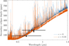 |
Fig. 2 Theoretical occultation spectra of WASP-189b for two different values of the heat-redistribution factor, ϵ. The squares represent the bandpass-integrated occultation depths in the CHEOPS and TESS bandpasses based on the theoretical model calculations. The observational data is shown in black. |
3.2.2 Thermal structure of the atmosphere
One of the advantages of using the phase curve model of Cowan & Agol (2008) is that we can invert the model (Eq. (4)) to find the planetary brightness as a function of longitude (ϕ) and latitude (θ), I(ϕ, θ). First, we can compute a longitudinal surface brightness map, J(ϕ), expressed as (Cowan & Agol 2008; Kempton et al. 2023):
![Mathematical equation: $\[J(\phi)=A_0+A_1 ~\cos~ \phi+B_1 ~\sin~ \phi+A_2 ~\cos~ 2 \phi+B_2 ~\sin~ 2 \phi.\]$](/articles/aa/full_html/2026/02/aa57139-25/aa57139-25-eq28.png) (11)
(11)
Here, we have
![Mathematical equation: $\[\begin{aligned}& A_0=\left(E-C_1-C_2\right) / 2, \\& A_1=2 C_1 / \pi, \\& B_1=-2 D_1 / \pi, \\& A_2=3 C_2 / 2, \\& B_2=-3 D_2 / 2.\end{aligned}\]$](/articles/aa/full_html/2026/02/aa57139-25/aa57139-25-eq29.png) (12)
(12)
Here, E, C1, D1, D2, and D2 are phase curve parameters from Eq. (4). We note here that our phase curve observations can only estimate the longitudinal distribution of the planetary flux, while the latitudinal distribution remains unconstrained. We can make several assumptions, for instance, negligible brightness from the planetary poles and sinusoidal variation of brightness along latitude, to obtain a 2D brightness map, I(ϕ, θ). Following Dang et al. (2018); Keating et al. (2019), we have
![Mathematical equation: $\[I(\phi, \theta)=\frac{3}{4} \cdot J(\phi) \cdot \sin~ (\theta+\pi / 2).\]$](/articles/aa/full_html/2026/02/aa57139-25/aa57139-25-eq30.png) (13)
(13)
Here, we add π/2 to θ in the above equation since we have taken θ = ±π/2 at poles and θ = 0 at the equator. The top panel of Fig. 3 shows the brightness variation along the equator of the planet, Ieq = I(ϕ, θ = 0). As we can see, the maximum emission comes from the longitudes near the substellar point (i.e. 0°), while the emission is consistent with zero towards nightside longitudes (i.e. near ±180°). This indicates that, as mentioned earlier in this paper, there is very little phase offset and a huge contrast between the flux emitted from the dayside and the nightside.
As described in Sect. 3.2.1, we mainly see planetary thermal emission in our TESS bandpass. We can use this information, along with an assumption of the planet’s emission as a blackbody, to translate the derived I(ϕ, θ) to a temperature map of the planet, Tp(ϕ, θ). We assume the planet emits as a blackbody without any absorption or emission due to chemical species from the atmosphere of the planet. This simplification is needed because we do not know the planetary emission spectrum. We use Planck’s law to invert I(ϕ, θ) to obtain Tp(ϕ, θ). The I(ϕ, θ) gives negative values of flux at some of the nightside longitudes, which is not physical. We set the temperature of these negative fluxes to 0 K while computing the temperature distribution. The temperature distribution at the equator is shown in the middle panel of Fig. 3. As can be seen, the temperature difference between the substellar point (0°) and the morning-evening terminator (±90°) is large (~1000 K). The full median 2D temperature map derived from median I(ϕ, θ) (Eq. (13)) is shown in the bottom panel of Fig. 3. With certain caveats that were described above, this 2D temperature map gives a complete description of the thermal structure of the planet at the altitudes probed by TESS wavelengths.
We can calculate the Bond albedo and heat redistribution efficiency given the 2D temperature maps. The Bond albedo can be estimated as (Keating et al. 2019; Kempton et al. 2023):
![Mathematical equation: $\[A_B=1-\frac{a^2}{\pi T_{\star}^4 R_{\star}^2} \iint T_p^4(\phi, \theta) ~\sin~ \theta d ~\theta ~d \phi.\]$](/articles/aa/full_html/2026/02/aa57139-25/aa57139-25-eq31.png) (14)
(14)
Here, a/R⋆ is the scaled semi-major axis, T⋆ is the stellar effective temperature, and Tp(ϕ, θ) is the 2D temperature distribution as a function of longitude (ϕ) and latitude (θ). We calculated AB = ![Mathematical equation: $\[0.35_{-0.07}^{+0.06}\]$](/articles/aa/full_html/2026/02/aa57139-25/aa57139-25-eq32.png) from our observations, which is mostly overestimated because of the underestimated integral in the above equation. This happens because our observations could not constrain Tp(ϕ, θ) for many nightside longitudes, where we put Tp(ϕ, θ) = 0. Therefore, the value of AB quoted above should be taken as an upper limit. We estimate a proper lower limit by recalculating AB from Eq. (14), but this time, we replace all unconstrained Tp(ϕ, θ) with the median temperature of the nightside region where we could constrain Tp(ϕ, θ). We get AB=
from our observations, which is mostly overestimated because of the underestimated integral in the above equation. This happens because our observations could not constrain Tp(ϕ, θ) for many nightside longitudes, where we put Tp(ϕ, θ) = 0. Therefore, the value of AB quoted above should be taken as an upper limit. We estimate a proper lower limit by recalculating AB from Eq. (14), but this time, we replace all unconstrained Tp(ϕ, θ) with the median temperature of the nightside region where we could constrain Tp(ϕ, θ). We get AB= ![Mathematical equation: $\[0.19_{-0.07}^{+0.07}\]$](/articles/aa/full_html/2026/02/aa57139-25/aa57139-25-eq33.png) , in this case, which is consistent with zero at 3σ. Therefore, the expected median range of AB from our observations is 0.19–0.35, with 3σ upper and lower limits are 0.53 and −0.02, respectively.
, in this case, which is consistent with zero at 3σ. Therefore, the expected median range of AB from our observations is 0.19–0.35, with 3σ upper and lower limits are 0.53 and −0.02, respectively.
We can estimate heat redistribution efficiency as the ratio of nightside flux to the dayside flux (e.g. Morris et al. 2022):
![Mathematical equation: $\[\varepsilon=\frac{\int_{\pi / 2}^{-\pi / 2} \int_{-\pi / 2}^{\pi / 2} F_p(\phi, \theta) ~\sin~ (\theta+\pi / 2) d \theta ~d \phi}{\int_{-\pi / 2}^{\pi / 2} \int_{-\pi / 2}^{\pi / 2} F_p(\phi, \theta) ~\sin~ (\theta+\pi / 2) d \theta ~d \phi}.\]$](/articles/aa/full_html/2026/02/aa57139-25/aa57139-25-eq34.png) (15)
(15)
Here, Fp(ϕ, θ) is the total emitted flux at longitude, ϕ, and latitude, θ, which we can calculate as ![Mathematical equation: $\[F_{p}(\phi, \theta)=\sigma_{\mathrm{sb}} T_{p}^{4}(\phi, \theta)\]$](/articles/aa/full_html/2026/02/aa57139-25/aa57139-25-eq35.png) , where σsb is Stefan-Boltzmann’s constant. We estimated ε =
, where σsb is Stefan-Boltzmann’s constant. We estimated ε = ![Mathematical equation: $\[0.09_{-0.04}^{+0.06}\]$](/articles/aa/full_html/2026/02/aa57139-25/aa57139-25-eq36.png) from our observations. Again, since we cannot constrain nightside temperatures properly, this value of ε is likely a lower limit. We compute an upper limit using the same method described previously in the case of AB, and find ε =
from our observations. Again, since we cannot constrain nightside temperatures properly, this value of ε is likely a lower limit. We compute an upper limit using the same method described previously in the case of AB, and find ε = ![Mathematical equation: $\[0.41_{-0.05}^{+0.06}\]$](/articles/aa/full_html/2026/02/aa57139-25/aa57139-25-eq37.png) , resulting in an expected median range of 0.09–0.41. The 3σ upper and lower limits on ε would be 0.59 and −0.03, respectively. Such heat redistribution efficiency is expected for ultra-hot Jupiters, where the dissociation and recombination of hydrogen increase the day–night heat transport.
, resulting in an expected median range of 0.09–0.41. The 3σ upper and lower limits on ε would be 0.59 and −0.03, respectively. Such heat redistribution efficiency is expected for ultra-hot Jupiters, where the dissociation and recombination of hydrogen increase the day–night heat transport.
We can further compute disk-integrated dayside and nightside effective temperatures of the planet (Keating et al. 2019):
![Mathematical equation: $\[\begin{aligned}T_{\text {day }}^4 & =\frac{1}{2 \pi} \int_{-\pi / 2}^{\pi / 2} \int_{-\pi / 2}^{\pi / 2} T^4(\phi, \theta) ~\sin~ \theta~ d \theta ~d \phi, \\T_{\text {night }}^4 & =\frac{1}{2 \pi} \int_{\pi / 2}^{-\pi / 2} \int_{-\pi / 2}^{\pi / 2} T^4(\phi, \theta) ~\sin~ \theta~ d \theta ~d \phi.\end{aligned}\]$](/articles/aa/full_html/2026/02/aa57139-25/aa57139-25-eq38.png) (16)
(16)
Here, T(ϕ, θ) is the 2D temperature map inverted from our observationally derived I(ϕ, θ) (Eq. (13)). We estimate Tday = ![Mathematical equation: $\[2746_{-45}^{+40}\]$](/articles/aa/full_html/2026/02/aa57139-25/aa57139-25-eq39.png) K and Tnight =
K and Tnight = ![Mathematical equation: $\[1529_{-209}^{+222}\]$](/articles/aa/full_html/2026/02/aa57139-25/aa57139-25-eq40.png) K. The latter of which is likely underestimated since we cannot properly constrain the nightside flux. Keating et al. (2019) studied the thermal structure of several hot Jupiters and showed that most of them show a uniform nightside temperature of about 1100 K, primarily because of the presence of clouds. With increasing stellar irradiation, the clouds can disperse, increasing the nightside temperature of highly irradiated planets. The nightside temperature of WASP-189b nicely fits in the trend found by Keating et al. (2019). Finally, we note that the physical quantities derived here depend on the temperature map of the planet, which, in turn, depends on the phase curve model we used.
K. The latter of which is likely underestimated since we cannot properly constrain the nightside flux. Keating et al. (2019) studied the thermal structure of several hot Jupiters and showed that most of them show a uniform nightside temperature of about 1100 K, primarily because of the presence of clouds. With increasing stellar irradiation, the clouds can disperse, increasing the nightside temperature of highly irradiated planets. The nightside temperature of WASP-189b nicely fits in the trend found by Keating et al. (2019). Finally, we note that the physical quantities derived here depend on the temperature map of the planet, which, in turn, depends on the phase curve model we used.
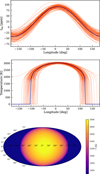 |
Fig. 3 Brightness and temperature maps of the planet. Top: equatorial brightness in the units of stellar brightness as a function of longitude. Middle: 1D temperature distribution on planetary equator as a function of planetary longitude. Bottom: median 2D latitude-longitude temperature map of the planet. The dark blue and orange lines in the top and middle plots show the median and randomly selected models from the posterior distribution. |
3.2.3 On the contribution of reflected light
Our atmospheric modelling (Sect. 3.2.1) suggests that the contribution of reflected light in both TESS and CHEOPS bandpasses is low. This is corroborated by our computation of Bond albedo, the lower limit of which we found to be consistent with zero at 3σ (Sect. 3.2.2). The optical bandpass of CHEOPS is better suited to constrain the geometric albedo of WASP-189 b. Deline et al. (2022), who observed optical CHEOPS phase curves and occultations, suggested that their observations can be explained by AB = 0, in the extreme case. However, they also considered that the reflected light contribution to the emission in the CHEOPS bandpass could be non-zero because it would require a negative Bond albedo to obtain the observed occultation depth only from thermal emission. We argue that the negative Bond albedo arises because of the inherently flawed nature of their 0D model (from Cowan & Agol 2011). Morris et al. (2022) showed that such 0D models can give negative Bond albedos in certain situations because of global non-conservation of energy. They further recommended using 2D temperature maps to calculate Bond albedo. Indeed, we show that our phase curve model and subsequently derived temperature maps, when applied to CHEOPS observations, give a small non-negative Bond albedo as expected.
For the purposes of this analysis, we analysed four occultations and two phase-curve observations from CHEOPS published by Lendl et al. (2020); Deline et al. (2022). This analysis was performed using the CHEOPS data alone. Since we were only interested in phase curves, we masked all transits present in the data. Our planetary model is the same as the one described in Sect. 2.3. There is a strong instrumental noise in CHEOPS data as mentioned by Deline et al. (2022). We fit a model similar to Deline et al. (2022) to model the instrumental noise. This model included a Fourier series up to fifth order for occultations and phase curves to fit roll-angle modulation, linear (for phase curves), and quadratic polynomials (for occultations) in time to model long-term trends and a linear model in thermFront_2 parameter to account for the flux ramp. Finally, we fit a GP model built from an SHO kernel implemented in celerite2 (Foreman-Mackey et al. 2017; Foreman-Mackey 2018) to the phase curve data to model the stellar noise (Deline et al. 2022). We fixed all the planetary parameters, except for phase curve parameters, to their values from Deline et al. (2022) in this analysis.
The detrended data along with the median and the models generated from the randomly selected posteriors are shown in the top panel of Fig. 4. Our constrained values of occultation depth, nightside flux and phase offset (![Mathematical equation: $\[93.9_{-1.9}^{+2.1}\]$](/articles/aa/full_html/2026/02/aa57139-25/aa57139-25-eq41.png) ppm,
ppm, ![Mathematical equation: $\[-6.7_{-17.1}^{+15.9}\]$](/articles/aa/full_html/2026/02/aa57139-25/aa57139-25-eq42.png) ppm, and
ppm, and ![Mathematical equation: $\[-5.6_{-6.9}^{+8.7}\]$](/articles/aa/full_html/2026/02/aa57139-25/aa57139-25-eq43.png) deg) are consistent with their values from Deline et al. (2022). We get smaller uncertainties on these parameters because we fixed planetary parameters in our analysis. We then used the formalism presented in Sect. 3.2.2 to invert this phase curve to find the brightness distribution, I(ϕ, θ), and temperature distribution of the planet. The median temperature distribution is shown in the bottom panel of Fig. 4. Again, where the planetary flux is not properly constrained (i.e. on the nightside where we get I(ϕ, θ) < 0 for some longitudes), we set Tp(ϕ, θ) = 0 (e.g. dark blue bands in Fig. 4). We estimated the Bond albedo, AB =
deg) are consistent with their values from Deline et al. (2022). We get smaller uncertainties on these parameters because we fixed planetary parameters in our analysis. We then used the formalism presented in Sect. 3.2.2 to invert this phase curve to find the brightness distribution, I(ϕ, θ), and temperature distribution of the planet. The median temperature distribution is shown in the bottom panel of Fig. 4. Again, where the planetary flux is not properly constrained (i.e. on the nightside where we get I(ϕ, θ) < 0 for some longitudes), we set Tp(ϕ, θ) = 0 (e.g. dark blue bands in Fig. 4). We estimated the Bond albedo, AB = ![Mathematical equation: $\[0.19_{-0.10}^{+0.06}\]$](/articles/aa/full_html/2026/02/aa57139-25/aa57139-25-eq44.png) , from this temperature map, which we found to be consistent with zero at ~2σ. As we could not constrain the nightside temperatures properly, the real value of AB is likely to be much lower than the value we report here (as also marked by its large uncertainty at the lower bound). To properly account for this, we set the temperature of the unconstrained nightside region to the median nightside temperature. We get AB =
, from this temperature map, which we found to be consistent with zero at ~2σ. As we could not constrain the nightside temperatures properly, the real value of AB is likely to be much lower than the value we report here (as also marked by its large uncertainty at the lower bound). To properly account for this, we set the temperature of the unconstrained nightside region to the median nightside temperature. We get AB = ![Mathematical equation: $\[0.05_{-0.03}^{+0.04}\]$](/articles/aa/full_html/2026/02/aa57139-25/aa57139-25-eq45.png) , making the expected median range of AB, 0.05–0.19. The 3σ upper and lower limits of AB are 0.37 and −0.04, respectively. Such low values of Bond albedo could mean that the contribution of reflective light in the CHEOPS bandpass is minimal. This is also hinted at by our atmospheric modelling (see Sect. 3.2.1). However, it is hard to calculate the exact contribution of reflected light in both TESS and CHEOPS bandpasses in the absence of a true spectrum.
, making the expected median range of AB, 0.05–0.19. The 3σ upper and lower limits of AB are 0.37 and −0.04, respectively. Such low values of Bond albedo could mean that the contribution of reflective light in the CHEOPS bandpass is minimal. This is also hinted at by our atmospheric modelling (see Sect. 3.2.1). However, it is hard to calculate the exact contribution of reflected light in both TESS and CHEOPS bandpasses in the absence of a true spectrum.
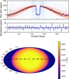 |
Fig. 4 CHEOPS phase curve and inferred temperature map from it. Top: detrended and phase-folded CHEOPS data along with the median (dark blue line) and models computed from randomly selected posteriors (orange line). Middle: residuals after subtracting the median model. The light and dark blue points show the unbinned and binned data, respectively. Bottom: derived median temperature map as a function of latitude and longitude. |
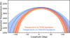 |
Fig. 5 Equatorial temperatures as a function of longitude as observed by TESS (orange) and CHEOPS (blue) bandpasses. The solid lines give median values of temperatures, while the shaded regions show the bands of 1σ uncertainty in temperatures. Some nightside longitudes are not shown since our modelling is not able to properly constrain temperatures on very high longitudes. |
3.2.4 Bandpass dependent thermal structure
We computed the temperature distribution of WASP-189b in two different bandpasses. TESS and CHEOPS bandpasses, while overlapping at large wavelengths, are sensitive to slightly different wavelengths, with the CHEOPS bandpass being more sensitive to bluer wavelengths than the TESS bandpass. They naturally probe different atmospheric layers in the atmosphere of the planet. Comparing temperature distribution constrained by both bandpasses can give hints as to how the thermal structure varies with altitude in the atmosphere.
Figure 5 shows the equatorial temperatures as a function of longitude as observed by TESS and CHEOPS. As we can see, the estimated temperatures are almost similar in both bandpasses. However, the temperature is slightly higher in the CHEOPS bandpass compared to the TESS bandpass. This could be explained by the presence of short-wave absorbers such as titanium oxide (TiO) in the atmosphere of WASP-189b (Prinoth et al. 2022, 2023). Such short-wave absorbers can create a temperature inversion in the atmosphere, which was indeed empirically found by Lesjak et al. (2025) for WASP-189b. The existence of short-wave absorbers also means that the radiation detected by the bluer bandpass of CHEOPS is radiated by the upper, hotter layers. On the other hand, TESS’s redder bandpass receives radiation from slightly deeper and, thus, cooler, layers. This could explain the temperature difference in the CHEOPS and TESS bandpasses. Given that both bandpasses overlap for a large wavelength range, the temperature difference is small, as seen in Fig. 5.
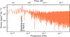 |
Fig. 6 Lomb–Scargle periodogram of the TESS light curve after subtracting the instrumental noise. The bottom and upper axes of the figure show the frequency and time domain, respectively. The period range covered by the periodogram is from the period corresponding to the Nyquist frequency to the total duration of the observation. |
4 Stellar variability
Deline et al. (2022) found photometric variability in the CHEOPS phase curve of WASP-189b with the period of about 1.3 days. They attributed this photometric variability to stellar rotation since the period of variability was very close to the stellar rotation period, P⋆ = ![Mathematical equation: $\[1.22_{-0.03}^{+0.03}\]$](/articles/aa/full_html/2026/02/aa57139-25/aa57139-25-eq46.png) d. We recovered this photometric variability in our CHEOPS phase curve analysis presented in Sect. 3.2.3 (see the bottom panel of Fig. C.1 for our best-fit GP model to CHEOPS data). We fit a slightly larger undamped period of the process compared to Deline et al. (2022, see our Table C.1). Given the presence of photometric variability in CHEOPS data, we searched for the same in the TESS data. The longer observing baseline the TESS data provides is especially suitable for determining the long-term variability of WASP-189. Figure 6 shows the Lomb-Scargle periodogram of the TESS data after subtracting the instrumental noise and masking transits and occultations. The periodogram has one significant peak at 2.74 d, which, although much larger than the period of photometric variability found by Deline et al. (2022), is consistent with the orbital period of the planet (P = 2.72 d). Therefore, we think that the peak corresponds to the planetary phase-curve signal rather than any stellar variability. Curiously, in contrast to what was repoted by Deline et al. (2022), there are no significant peaks around 1.2 days. The photometric variability discovered by CHEOPS seems to be absent in the TESS data. We note here that the TESS data is less precise compared to the CHEOPS data: we estimate the photometric precision of both datasets by calculating MAD of residuals, found by subtracting best-fit model from the raw flux, binned over 1 h. We found 12.76 ppm and 47.59 ppm in 1 hr for CHEOPS and TESS datasets, respectively. It is possible that the stellar photometric variability is not visible because of noise in the TESS data.
d. We recovered this photometric variability in our CHEOPS phase curve analysis presented in Sect. 3.2.3 (see the bottom panel of Fig. C.1 for our best-fit GP model to CHEOPS data). We fit a slightly larger undamped period of the process compared to Deline et al. (2022, see our Table C.1). Given the presence of photometric variability in CHEOPS data, we searched for the same in the TESS data. The longer observing baseline the TESS data provides is especially suitable for determining the long-term variability of WASP-189. Figure 6 shows the Lomb-Scargle periodogram of the TESS data after subtracting the instrumental noise and masking transits and occultations. The periodogram has one significant peak at 2.74 d, which, although much larger than the period of photometric variability found by Deline et al. (2022), is consistent with the orbital period of the planet (P = 2.72 d). Therefore, we think that the peak corresponds to the planetary phase-curve signal rather than any stellar variability. Curiously, in contrast to what was repoted by Deline et al. (2022), there are no significant peaks around 1.2 days. The photometric variability discovered by CHEOPS seems to be absent in the TESS data. We note here that the TESS data is less precise compared to the CHEOPS data: we estimate the photometric precision of both datasets by calculating MAD of residuals, found by subtracting best-fit model from the raw flux, binned over 1 h. We found 12.76 ppm and 47.59 ppm in 1 hr for CHEOPS and TESS datasets, respectively. It is possible that the stellar photometric variability is not visible because of noise in the TESS data.
Although we did not detect any short-term variability akin to that found in CHEOPS, the periodogram shows enhanced power at lower frequencies, indicating the presence of long-term noise. Given the amount of noise in the raw data, this is likely to be leftover instrumental noise. Therefore, we added a GP model built from an SHO kernel to model the additional correlated noise (see Sect. 2.4 for the details). The best-fit GP model is shown in the top panel of Fig. C.1. The GP model can produce oscillations if the quality factor, Q, of the GP is greater than 0.5 (i.e., ln Q > −0.69). The fitted Q value of the GP is below this threshold (see Table C.1), so we do not see regular oscillations in the model. The best-fit undamped period of the GP is ![Mathematical equation: $\[0.55_{-0.27}^{+0.36}\]$](/articles/aa/full_html/2026/02/aa57139-25/aa57139-25-eq47.png) d, which gives the damped period of
d, which gives the damped period of ![Mathematical equation: $\[2.19_{-0.44}^{+1.35}\]$](/articles/aa/full_html/2026/02/aa57139-25/aa57139-25-eq48.png) d (or,
d (or, ![Mathematical equation: $\[52.63_{-10.48}^{+32.48}\]$](/articles/aa/full_html/2026/02/aa57139-25/aa57139-25-eq49.png) hr). Although the stellar properties of WASP-189 situate it in a parameter space where δ-Scuti and γ-Doradus stars are found, the irregularities of the fitted GP model mean that the noise is not likely of stellar origin.
hr). Although the stellar properties of WASP-189 situate it in a parameter space where δ-Scuti and γ-Doradus stars are found, the irregularities of the fitted GP model mean that the noise is not likely of stellar origin.
5 Conclusions
We analysed the new TESS and archival CHEOPS phase curves to investigate the orbital architecture and thermal structure of an ultra-hot Jupiter WASP-189b. Our main conclusions are listed below:
Our analysis of gravity-darkened transit allowed us to examine the orbital architecture. We found, in agreement with Deline et al. (2022), that the planet is in a polar orbit around its host star, with the 3D spin-orbit angle being
![Mathematical equation: $\[89.46_{-1.08}^{+1.08}\]$](/articles/aa/full_html/2026/02/aa57139-25/aa57139-25-eq50.png) deg;
deg;The whole dataset, including archival CHEOPS data and TESS data, spans roughly two years. We used this data over a long baseline to see if there is orbital precession because of stellar oblateness. We found that our impact parameter and projected orbital obliquity are consistent with their corresponding values from archival CHEOPS data, as well as with their rate of changes,
![Mathematical equation: $\[-1.59_{-39.35}^{+38.77}\]$](/articles/aa/full_html/2026/02/aa57139-25/aa57139-25-eq51.png) × 10−6 yr−1 and
× 10−6 yr−1 and ![Mathematical equation: $\[-0.0026_{-0.0043}^{+0.0058}\]$](/articles/aa/full_html/2026/02/aa57139-25/aa57139-25-eq52.png) deg yr−1, respectively, consistent with zero. This suggests an absence of a fast orbital precession;
deg yr−1, respectively, consistent with zero. This suggests an absence of a fast orbital precession;We detected a significant phase curve with an occultation depth of
![Mathematical equation: $\[203.4_{-16.3}^{+16.2}\]$](/articles/aa/full_html/2026/02/aa57139-25/aa57139-25-eq53.png) ppm, a negative, yet consistent with zero, nightside flux (Fn/F⋆ =
ppm, a negative, yet consistent with zero, nightside flux (Fn/F⋆ = ![Mathematical equation: $\[-71.8_{-36.0}^{+36.4}\]$](/articles/aa/full_html/2026/02/aa57139-25/aa57139-25-eq54.png) ppm), and a negligible phase offset of
ppm), and a negligible phase offset of ![Mathematical equation: $\[-9.78_{-6.82}^{+6.81}\]$](/articles/aa/full_html/2026/02/aa57139-25/aa57139-25-eq55.png) deg. Our atmospheric forward models of thermal emission with minor contribution from reflected light in an atmosphere with inefficient heat transport can explain the observed occultation depths in both TESS and CHEOPS bandpasses;
deg. Our atmospheric forward models of thermal emission with minor contribution from reflected light in an atmosphere with inefficient heat transport can explain the observed occultation depths in both TESS and CHEOPS bandpasses;Our phase-curve model enabled us to invert the phase curve to find temperature maps of the planet, which we calculated for both TESS and CHEOPS bandpasses. Upon comparing temperature maps in both bandpasses, we found that, while the temperatures are almost similar in both bands, it is slightly higher in the CHEOPS band compared to the TESS band throughout the dayside. A temperature inversion, caused by previously detected short-wave absorbers such as TiO, could readily explain this (Prinoth et al. 2022, 2023);
We used temperature maps to estimate the Bond albedo (AB) in TESS and CHEOPS bandpasses. Given the unconstrained nightside temperatures, we could derive accepted median ranges of AB, 0.19–0.35 in the TESS bandpass and 0.05–0.19 in the CHEOPS bandpass. We also derived 3σ upper and lower limits of AB for both bandpasses. Similarly, we constrained the heat re-distribution efficiency in the 0.09–0.41 median range for the TESS bandpass;
Deline et al. (2022) detected a long-term photometric variability at the period of about 1.3 days, which they attributed to the stellar rotation. We did not detect a similar photometric variability in our TESS observations. This may be because of the lower photometric precision of the TESS data compared to the CHEOPS observations. However, we detected correlated noise of unknown origin.
Our phase curve observations primarily have the ability to constrain the longitudinal thermal structure. We made additional assumptions to obtain a 2D latitude-longitude thermal structure of the atmosphere. However, it is possible to directly constrain 2D latitude-longitude thermal structure with ultra-precise occultation observations. Moreover, spectroscopic observations can provide altitude information, which helps improve our understanding of 3D atmospheric structure. Observations with the JWST can help us achieve this (Hammond et al. 2024). This type of 3D atmospheric structure is crucial for studying not only the thermal structure, but also atmospheric dynamics.
Acknowledgements
We would like to thank an anonymous referee for their detailed referee report and suggestions which significantly improved the manuscript. JAP and ABr were supported by SNSA. DK acknowledges financial support from the Center for Space and Habitability (CSH) of the University of Bern. TWi acknowledges support from the UKSA and the University of Warwick. ADe has received funding from the Swiss National Science Foundation for project 200021_200726 ML acknowledges support of the Swiss National Science Foundation under grant number PCEFP2_194576. The contributions of ML and ADe have been carried out within the framework of the NCCR PlanetS supported by the Swiss National Science Foundation under grant 51NF40_205606. VS acknowledge support from CHEOPS ASI-INAF agreement no. 2019-29-HH.0.
Appendix A Planetary and stellar parameters
Planetary and stellar parameters used in the light curve analysis.
Appendix B TESS light curves of WASP-189 b reduced from PDC-SAP and SCALPELS pipeline
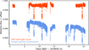 |
Fig. B.1 Light curves of WASP-189b reduced from two pipelines. The PDC-SAP light curve produced by TESS SPOC is shown in orange, and the light curve extracted using our manual SCALPLES pipeline is shown in blue. |
Appendix C GP models
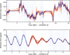 |
Fig. C.1 Best-fit GP models to the TESS (top) and CHEOPS (bottom) data. The light and dark blue points are unbinned and binned data points, respectively. The solid blue and orange lines give the median GP model and models generated from randomly selected posteriors. |
GP parameters used in the light curve analysis.
References
- Anderson, D. R., Temple, L. Y., Nielsen, L. D., et al. 2018, arXiv e-prints [arXiv:1809.04897] [Google Scholar]
- Arcangeli, J., Désert, J.-M., Line, M. R., et al. 2018, ApJ, 855, L30 [Google Scholar]
- Barnes, J. W. 2009, ApJ, 705, 683 [Google Scholar]
- Bell, T. J., & Cowan, N. B. 2018, ApJ, 857, L20 [Google Scholar]
- Benz, W., Broeg, C., Fortier, A., et al. 2021, Exp. Astron., 51, 109 [Google Scholar]
- Coulombe, L.-P., Benneke, B., Challener, R., et al. 2023, Nature, 620, 292 [NASA ADS] [CrossRef] [Google Scholar]
- Cowan, N. B., & Agol, E. 2008, ApJ, 678, L129 [Google Scholar]
- Cowan, N. B., & Agol, E. 2011, ApJ, 729, 54 [Google Scholar]
- Dang, L., Cowan, N. B., Schwartz, J. C., et al. 2018, Nat. Astron., 2, 220 [NASA ADS] [CrossRef] [Google Scholar]
- Deibert, E. K., Langeveld, A. B., Young, M. E., et al. 2024, AJ, 168, 148 [Google Scholar]
- Deline, A., Hooton, M. J., Lendl, M., et al. 2022, A&A, 659, A74 [NASA ADS] [CrossRef] [EDP Sciences] [Google Scholar]
- Deline, A., Cubillos, P. E., Carone, L., et al. 2025, A&A, 699, A150 [NASA ADS] [CrossRef] [EDP Sciences] [Google Scholar]
- Deming, D., Knutson, H., Kammer, J., et al. 2015, ApJ, 805, 132 [Google Scholar]
- Foreman-Mackey, D. 2018, RNAAS, 2, 31 [NASA ADS] [Google Scholar]
- Foreman-Mackey, D., Agol, E., Ambikasaran, S., & Angus, R. 2017, AJ, 154, 220 [Google Scholar]
- Hammond, M., Bell, T. J., Challener, R. C., et al. 2024, AJ, 168, 4 [Google Scholar]
- Hamre, B., Stamnes, S., Stamnes, K., & Stamnes, J. J. 2013, in Radiation Processes in the Atmosphere and Ocean, American Institute of Physics Conference Series, 1531, American Institute of Physics Conference Series, eds. R. Cahalan & J. Fischer, 923 [Google Scholar]
- Heng, K., & Showman, A. P. 2015, Annu. Rev. Earth Planet. Sci., 43, 509 [CrossRef] [Google Scholar]
- Heng, K., Morris, B. M., & Kitzmann, D. 2021, Nat. Astron., 5, 1001 [NASA ADS] [CrossRef] [Google Scholar]
- Higson, E., Handley, W., Hobson, M., & Lasenby, A. 2019, Statist. Comput., 29, 891 [Google Scholar]
- Hooton, M. J., Hoyer, S., Kitzmann, D., et al. 2022, A&A, 658, A75 [NASA ADS] [CrossRef] [EDP Sciences] [Google Scholar]
- Husser, T. O., Wende-von Berg, S., Dreizler, S., et al. 2013, A&A, 553, A6 [NASA ADS] [CrossRef] [EDP Sciences] [Google Scholar]
- Jenkins, J. M., Twicken, J. D., McCauliff, S., et al. 2016, SPIE Conf. Ser., 9913, 99133E [Google Scholar]
- Johnson, M. C., Cochran, W. D., Collier Cameron, A., & Bayliss, D. 2015, ApJ, 810, L23 [Google Scholar]
- Jones, K., Morris, B. M., Demory, B. O., et al. 2022, A&A, 666, A118 [NASA ADS] [CrossRef] [EDP Sciences] [Google Scholar]
- Keating, D., Cowan, N. B., & Dang, L. 2019, Nat. Astron., 3, 1092 [NASA ADS] [CrossRef] [Google Scholar]
- Kempton, E. M. R., Zhang, M., Bean, J. L., et al. 2023, Nature, 620, 67 [NASA ADS] [CrossRef] [Google Scholar]
- Kipping, D. M. 2013, MNRAS, 435, 2152 [Google Scholar]
- Kitzmann, D., Heng, K., Rimmer, P. B., et al. 2018, ApJ, 863, 183 [Google Scholar]
- Kitzmann, D., Stock, J. W., & Patzer, A. B. C. 2024, MNRAS, 527, 7263 [Google Scholar]
- Komacek, T. D., & Showman, A. P. 2016, ApJ, 821, 16 [CrossRef] [Google Scholar]
- Lendl, M., Csizmadia, S., Deline, A., et al. 2020, A&A, 643, A94 [EDP Sciences] [Google Scholar]
- Lesjak, F., Nortmann, L., Cont, D., et al. 2025, A&A, 693, A72 [NASA ADS] [CrossRef] [EDP Sciences] [Google Scholar]
- Lothringer, J. D., Barman, T., & Koskinen, T. 2018, ApJ, 866, 27 [NASA ADS] [CrossRef] [Google Scholar]
- Luger, R., Agol, E., Kruse, E., et al. 2016, AJ, 152, 100 [Google Scholar]
- Malik, M., Grosheintz, L., Mendonça, J. M., et al. 2017, AJ, 153, 56 [Google Scholar]
- Malik, M., Kitzmann, D., Mendonça, J. M., et al. 2019, AJ, 157, 170 [Google Scholar]
- Mansfield, M., Bean, J. L., Line, M. R., et al. 2018, AJ, 156, 10 [NASA ADS] [CrossRef] [Google Scholar]
- Mansfield, M., Bean, J. L., Stevenson, K. B., et al. 2020, ApJ, 888, L15 [Google Scholar]
- Mansfield, M., Line, M. R., Bean, J. L., et al. 2021, Nat. Astron., 5, 1224 [CrossRef] [Google Scholar]
- Masuda, K. 2015, ApJ, 805, 28 [NASA ADS] [CrossRef] [Google Scholar]
- Morris, B. M., Heng, K., Jones, K., et al. 2022, A&A, 660, A123 [NASA ADS] [CrossRef] [EDP Sciences] [Google Scholar]
- Parmentier, V., Line, M. R., Bean, J. L., et al. 2018, A&A, 617, A110 [NASA ADS] [CrossRef] [EDP Sciences] [Google Scholar]
- Parviainen, H. 2015, MNRAS, 450, 3233 [Google Scholar]
- Patel, J. A., & Espinoza, N. 2022, AJ, 163, 228 [NASA ADS] [CrossRef] [Google Scholar]
- Patel, J. A., Brandeker, A., Kitzmann, D., et al. 2024, A&A, 690, A159 [NASA ADS] [CrossRef] [EDP Sciences] [Google Scholar]
- Prinoth, B., Hoeijmakers, H. J., Kitzmann, D., et al. 2022, Nat. Astron., 6, 449 [NASA ADS] [CrossRef] [Google Scholar]
- Prinoth, B., Hoeijmakers, H. J., Pelletier, S., et al. 2023, A&A, 678, A182 [NASA ADS] [CrossRef] [EDP Sciences] [Google Scholar]
- Prinoth, B., Hoeijmakers, H. J., Morris, B. M., et al. 2024, A&A, 685, A60 [NASA ADS] [CrossRef] [EDP Sciences] [Google Scholar]
- Ricker, G. R., Winn, J. N., Vanderspek, R., et al. 2014, SPIE Conf. Ser., 9143, 914320 [Google Scholar]
- Sheppard, K. B., Mandell, A. M., Tamburo, P., et al. 2017, ApJ, 850, L32 [Google Scholar]
- Singh, V., Scandariato, G., Smith, A. M. S., et al. 2024, A&A, 683, A1 [NASA ADS] [CrossRef] [EDP Sciences] [Google Scholar]
- Skilling, J. 2004, in American Institute of Physics Conference Series, 735, Bayesian Inference and Maximum Entropy Methods in Science and Engineering: 24th International Workshop on Bayesian Inference and Maximum Entropy Methods in Science and Engineering, eds. R. Fischer, R. Preuss, & U. V. Toussaint, 395 [Google Scholar]
- Skilling, J. 2006, Bayesian Anal., 1, 833 [Google Scholar]
- Smith, J. C., Stumpe, M. C., Van Cleve, J. E., et al. 2012, PASP, 124, 1000 [Google Scholar]
- Sobolev, V. V. 1975, [arXiv:2512.05175] [Google Scholar]
- Speagle, J. S. 2020, MNRAS, 493, 3132 [Google Scholar]
- Sreejith, A. G., France, K., Fossati, L., et al. 2023, ApJ, 954, L23 [NASA ADS] [CrossRef] [Google Scholar]
- Stamnes, K., Tsay, S.-C., Jayaweera, K., & Wiscombe, W. 1988, Appl. Opt., 27, 2502 [NASA ADS] [CrossRef] [Google Scholar]
- Stevenson, K. B., Désert, J.-M., Line, M. R., et al. 2014, Science, 346, 838 [Google Scholar]
- Stephan, A. P., Wang, J., Cauley, P. W., et al. 2022, ApJ, 931, 111 [NASA ADS] [CrossRef] [Google Scholar]
- Stock, J. W., Kitzmann, D., Patzer, A. B. C., & Sedlmayr, E. 2018, MNRAS, 479, 865 [NASA ADS] [Google Scholar]
- Stock, J. W., Kitzmann, D., & Patzer, A. B. C. 2022, MNRAS, 517, 4070 [NASA ADS] [CrossRef] [Google Scholar]
- Stumpe, M. C., Smith, J. C., Catanzarite, J. H., et al. 2014, PASP, 126, 100 [Google Scholar]
- Szabó, G. M., Pál, A., Derekas, A., et al. 2012, MNRAS, 421, L122 [Google Scholar]
- Vaulato, V., Pelletier, S., Ehrenreich, D., et al. 2025, A&A, 700, A9 [NASA ADS] [CrossRef] [EDP Sciences] [Google Scholar]
- von Zeipel, H. 1924, MNRAS, 84, 684 [NASA ADS] [CrossRef] [Google Scholar]
- Watanabe, N., Narita, N., Palle, E., et al. 2022, MNRAS, 512, 4404 [NASA ADS] [CrossRef] [Google Scholar]
- Watanabe, N., Narita, N., & Hori, Y. 2024, PASJ, 76, 374 [NASA ADS] [CrossRef] [Google Scholar]
- Yan, F., Pallé, E., Reiners, A., et al. 2022, A&A, 661, L6 [NASA ADS] [CrossRef] [EDP Sciences] [Google Scholar]
All Tables
All Figures
|
Fig. 1 Detrended and phase-folded TESS data along with the best-fit model. The light and dark blue points show the unbinned and binned data points. The dark blue and orange lines are the median model and models computed from randomly selected posteriors, respectively. Top: full phase curve with a transit and occultation. Middle: zoom-in on the transit (middle left) and occultation/phase curve (middle right). The dashed line represents the level of stellar flux (i.e. flux level during the occultation). The gravity darkened asymmetric transit and a phase variation, along with an occultation, are clearly visible in the middle panel. Bottom: residuals after subtracting the median model from the raw data. |
| In the text | |
|
Fig. 2 Theoretical occultation spectra of WASP-189b for two different values of the heat-redistribution factor, ϵ. The squares represent the bandpass-integrated occultation depths in the CHEOPS and TESS bandpasses based on the theoretical model calculations. The observational data is shown in black. |
| In the text | |
|
Fig. 3 Brightness and temperature maps of the planet. Top: equatorial brightness in the units of stellar brightness as a function of longitude. Middle: 1D temperature distribution on planetary equator as a function of planetary longitude. Bottom: median 2D latitude-longitude temperature map of the planet. The dark blue and orange lines in the top and middle plots show the median and randomly selected models from the posterior distribution. |
| In the text | |
|
Fig. 4 CHEOPS phase curve and inferred temperature map from it. Top: detrended and phase-folded CHEOPS data along with the median (dark blue line) and models computed from randomly selected posteriors (orange line). Middle: residuals after subtracting the median model. The light and dark blue points show the unbinned and binned data, respectively. Bottom: derived median temperature map as a function of latitude and longitude. |
| In the text | |
|
Fig. 5 Equatorial temperatures as a function of longitude as observed by TESS (orange) and CHEOPS (blue) bandpasses. The solid lines give median values of temperatures, while the shaded regions show the bands of 1σ uncertainty in temperatures. Some nightside longitudes are not shown since our modelling is not able to properly constrain temperatures on very high longitudes. |
| In the text | |
|
Fig. 6 Lomb–Scargle periodogram of the TESS light curve after subtracting the instrumental noise. The bottom and upper axes of the figure show the frequency and time domain, respectively. The period range covered by the periodogram is from the period corresponding to the Nyquist frequency to the total duration of the observation. |
| In the text | |
|
Fig. B.1 Light curves of WASP-189b reduced from two pipelines. The PDC-SAP light curve produced by TESS SPOC is shown in orange, and the light curve extracted using our manual SCALPLES pipeline is shown in blue. |
| In the text | |
|
Fig. C.1 Best-fit GP models to the TESS (top) and CHEOPS (bottom) data. The light and dark blue points are unbinned and binned data points, respectively. The solid blue and orange lines give the median GP model and models generated from randomly selected posteriors. |
| In the text | |
Current usage metrics show cumulative count of Article Views (full-text article views including HTML views, PDF and ePub downloads, according to the available data) and Abstracts Views on Vision4Press platform.
Data correspond to usage on the plateform after 2015. The current usage metrics is available 48-96 hours after online publication and is updated daily on week days.
Initial download of the metrics may take a while.