© The Authors 2026

1. Introduction

The deflection of light rays due to the presence of matter between a source and the observer, known as weak gravitational lensing, has been established as one of the most powerful probes for exploring the nature of dark matter and dark energy. It can be used to constrain the parameters of the current, widely used cosmological model (Albrecht et al. 2006; Kilbinger 2015). In the 2010s, large-area weak lensing surveys (Stage III surveys) such as the Dark Energy Survey¹ (Abbott et al. 2018), Kilo-Degree Survey² (de Jong et al. 2013), and Hyper Suprime-Cam³ (Aihara et al. 2018) were developed. In recent years, their results (Heymans et al. 2021; Secco et al. 2022; Dalal et al. 2023; Li et al. 2023; Dark Energy Survey and Kilo-Degree Survey Collaboration 2023) have spurred a discussion of potential tensions in early- and late-time Universe cosmology (Abdalla et al. 2022), opening up new questions and paving the way for Stage IV surveys. Upcoming surveys include the Legacy Survey of Space and Time⁴ on the NSF-DOE Vera C. Rubin Observatory (Ivezić et al. 2019), the Euclid mission⁵ (Laureijs et al. 2011), and the Nancy Roman Space Telescope⁶ (Spergel et al. 2015), which allow for precision cosmology to be applied.

The main advantage of weak lensing over other probes of cosmic structure is that it is directly sensitive to mass and, thus, less affected by astrophysical uncertainties (Weinberg et al. 2013). However, it is susceptible to a number of potential systematic sources of error, which pose challenges for the use of such surveys. One of these sources of systematic error is the intrinsic alignments (IA) of galaxies, a term used to refer to the correlations between galaxy shapes and orientations with each other and the underlying density field due to local processes, such as tidal fields (Troxel & Ishak 2015; Joachimi et al. 2015; Lamman et al. 2024). These localised correlations are similar to the effects of cosmic shear and contaminate weak gravitational lensing observations (Krause et al. 2015). Therefore, to fully exploit the potential of weak lensing as a tool for precision cosmology, these non-lensing alignments must either be removed or modelled precisely (Joachimi & Bridle 2010; Zhang 2010; Troxel & Ishak 2011). For reviews on intrinsic alignments, we refer to Troxel & Ishak (2015), Joachimi et al. (2015), Kirk et al. (2015), Kiessling et al. (2015) and, for a practical guide, we refer to Lamman et al. (2024).

Apart from their importance as a source of systematic bias in weak lensing studies, there is cosmological information that can be extracted from the IA signal, allowing it to be used to improve our comprehension of the formation and evolution of the large-scale structure of the Universe (e.g. Chisari & Dvorkin 2013; Chisari et al. 2014; Schmidt et al. 2015; Biagetti & Orlando 2020; Akitsu et al. 2023; Okumura & Taruya 2023; Kurita & Takada 2023; Xu et al. 2023). Galaxies of different types, colours and in different environments are also sensitive to intrinsic alignments in different ways, likely connected to their evolution through mergers and torques (e.g. Bate et al. 2020; Bhowmick et al. 2020) and to baryonic processes (e.g. Velliscig et al. 2015; Tenneti et al. 2017; Soussana et al. 2020). These relations and effects are often studied using hydrodynamical simulations such as IllustrisTNG (Nelson et al. 2021), EAGLE (Schaye et al. 2015), Horizon-AGN (Dubois et al. 2014), and MassiveBlack-II (Khandai et al. 2015).

The results and insights obtained from hydrodynamical simulations can be used to calibrate analytical models and constrain the priors or their parameters. Analytical methods include the linear alignment model (Hirata & Seljak 2004), extended to incorporate non-linear contributions (Hirata et al. 2007; Bridle & King 2007), which is valid on large scales. Additionally, the halo model relates the IA signal at small scales to the distribution of matter in dark matter halos (Schneider & Bridle 2010; Fortuna et al. 2020) and the EFT model describes the IA signal at intermediate scales (Vlah et al. 2020).

For the optimal mitigation of the effects of IA on weak lensing surveys, the parameters of the models need to be determined as precisely as possible. We need to extract as much information as we can from simulations. The obvious route would be to run larger simulations, increasing the sample sizes and, therefore, decreasing the noise in the measurements. However, this is very computationally expensive, making other avenues worth investigating. In recent years, the avenue of finding the optimal estimator has been explored in multiple works. Along this line, Singh et al. (2024) developed a new multipole-based estimator that increases the precision of parameter fits to IA models by a factor of ∼2. Recently, Lamman et al. (2025) suggested an alternative approach, where the line-of-sight integration limit (Π_max) is varied with the separation, r_p. Similarly, Kumwembe et al. (2025) improved the S/N for multiplet alignments in DESI using imaging. In this work, we aim to find a complementary method to increase the amount of information that can be extracted from existing simulations, with a relative low computational cost and using the estimators already available. The main objective is to improve the S/N of intrinsic alignment correlations by considering a combination of the three possible projections over different axes of the simulation box. While previous works (e.g. Tenneti et al. 2020) have averaged over projections, the non-trivial cross-covariance between these projections has not been considered before, making the gain in S/N that can be obtained from combining multiple projections unknown. To gain an understanding of how this method complements different estimators, we considered two well-established estimators: w_g+ and the quadrupole, ${\stackrel{\sim }{\xi }}_{\mathrm{g}+,2}$ (Singh et al. 2024).

The rest of the work is structured as follows. In this study, we use one of the latest hydrodynamical simulations publicly available, the IllustrisTNG project, which will be described in more detail in Sect. 2, along with the sample selection. Section 3 discusses the methods adopted to calculate the shapes of galaxies and perform the two-point measurements, as well as the estimation of the covariance matrix through jackknife resampling and the calculation of the S/N values. Section 4 introduces the non-linear alignment model, used to fit the measurements. In Sect. 5, we present the results obtained from the applied methods. In Sect. 6, we discuss the results and outline potential avenues for future research and Sect. 7 summarises the conclusions drawn in this work.

2. Data

We used the IllustrisTNG hydrodynamic simulation. The particle and group data are described in the release papers by Springel et al. (2017) and Nelson et al. (2021).

2.1. IllustrisTNG

The IllustrisTNG cosmological simulations (hereafter TNG) are a series of large magnetohydrodynamical simulations of galaxy formation. These simulations are run using the moving-mesh code AREPO (Springel 2010). A Monte Carlo tracer particle scheme is utilised during the simulation to track the Lagrangian evolution of baryons (Genel et al. 2013). Each TNG simulation solves for the coupled evolution of dark matter, cosmic gas, luminous stars, and supermassive black holes from an initial redshift of z = 127 to z = 0.

The TNG simulations are based on a flat ΛCDM cosmological model, utilising parameters that are consistent with Planck Collaboration results, with a dark energy density of Ω_Λ, 0 = 0.6911, total matter density of Ω_m, 0 = 0.3089, baryon density of Ω_b, 0 = 0.0486, amplitude of the matter power spectrum of σ₈ = 0.8159, and n_s = 0.9667.

These initial parameters determine the distribution of dark matter and gas at high redshift (z = 127) within a periodic simulation box of a given volume. The simulations then evolve these conditions forward in time, following the gravitational interactions between dark matter and gas, as well as the hydrodynamics of the gas, using the AREPO code (Nelson et al. 2021). As the simulation progresses, dark matter and gas collapse into dense regions where stars can form. The simulation outputs snapshots at various redshifts, with a total of 100 snapshots. At each snapshot, the friends-of-friends (FoF) and SUBFIND algorithm are used to identify subhalos and, ultimately, galaxies (Springel et al. 2001).

The TNG project is made up of three simulations in periodic boxes with side lengths of 35,  75,  205 cMpc/h apiece and at different resolutions. In this work, we focus on TNG300 at the highest resolution (TNG300-1), which has 2500³ dark matter particles of a mass of m_DM = 5.9 × 10⁷ M_⊙ and a box size of (205 cMpc/h)³. In particular, we examined the snapshot at redshift zero. In the simulation, we looked at two distinct mass cuts for the shape sample, described in Sect. 2.2.

2.2. Sample Selection

To measure the cross-correlation between the galaxy positions and their shapes, we defined two galaxy shape samples and one galaxy position sample. In this study, the raw data come from the snapshot data catalogues of TNG300-1 at z = 0, sourced from publicly available data⁷. It is then processed using the equations and methods described in Sect. 3.

While simulated data are not subject to the same biases as observed data, such as the challenge of fitting ellipticities in the presence of pixel noise or imperfect PSF modelling (Samuroff et al. 2021), they remain susceptible to bias. This prompts us to implement quality cuts to ensure the validity of the conclusions that have been drawn. A primary source of uncertainty arises from galaxy resolution, which impacts the ellipticity and orientation measurements. Galaxies with an insufficient number of particles to provide a meaningful shape measurement affect the ellipticity distribution of the sample. Through a series of convergence tests, Chisari et al. (2015) found that a minimum number of 300 particles per galaxy would be needed to mitigate resolution bias to acceptable levels. Consequently, in this study, we followed this practice and applied a cut to the shape sample, selecting only galaxies with more than 300 particles.

For the position sample, we enforce a quality cut of n_★ > 50. This threshold reflects the minimum number of particles required for a bound substructure to be considered a legitimate galaxy by the SUBFIND algorithm used in the IllustrisTNG simulations (Nelson et al. 2021). Galaxies with fewer than 50 particles are not well-resolved and could be considered random fluctuations. These cuts leave a total of 192 109 galaxies in the shape sample and 371 855 in the position sample.

In addition to this quality cut, we also consider another shape sample defined by the galaxy stellar mass, M_★, enabling us to investigate whether the possible gain in S/N depends on the signal strength, as high mass galaxies have a stronger alignment signal. The high-mass shape sample is defined by M_★ > 10^10.5 M_⊙/h, and contains 24 430 galaxies. The choice in terms of the position sample remains the same.

3. Methodology

3.1. Galaxy shapes

To characterise the three-dimensional (3D) shape of a galaxy, we use both the simple and reduced inertia tensor. While the simple inertia tensor generally provides a higher IA correlation function signal amplitude, allowing for more insight in the workings of galaxies, the reduced inertia tensor shape gives more weight to particles closer to the centre. This leads to rounder estimates of galaxy shapes, which mimic the observations more closely and are, therefore, also worth studying (Tenneti et al. 2015). The simple (Eq. (1)) and reduced (Eq. (2)) tensors are given by

$$\begin{array}{cc}\hfill I_j^{k,l}& =\frac{1}{M_j}{\mathrm{\Sigma }}_{i=1}^{N_j}{m}_i{r}_i^k{r}_i^l,\hfill \end{array}$$(1)

$$\begin{array}{cc}\hfill I_j^{k,l}& =\frac{1}{M_j}{\mathrm{\Sigma }}_{i=1}^{N_j}\frac{m_i{r}_i^k{r}_i^l}{r^2},\hfill \end{array}$$(2)

where k, l run from 0 to 2 and denote the x, y, z components of a vector, r, and i runs over all N_j particles in galaxy, j. The vector, r, refers to the position of each particle (x_i) relative to the centre of mass (x_j), given by r_i = x_i − x_j. The centre of mass is measured via the mass weighted mean of the particle positions in a galaxy $({\mathbf{x}}_j=\frac{1}{M_j}{\mathrm{\Sigma }}_{i=1}^{N_j}{m}_i{\mathbf{x}}_i)$. The variables M_j and m_i refer to the galaxy and particle masses, respectively.

To determine the two-dimensional (2D) projected shapes of the galaxies, the positions of the particles are projected onto a plane, which can be given by either side of the simulation box. In most other studies, the xy plane is chosen arbitrarily, and thus Eq. (1) is projected along the z-axis by using only the k, l = 0, 1 elements, corresponding to x, y. For Eq. (2), r² is equal to r_x² + r_y², and so becomes the projected distance from the particle to the centre of mass.

In this work, we calculated three different 2D projected shapes by projecting onto the xy, xz, and yz planes, hereafter called the z, y and x projections, respectively, referring to the line-of-sight axis. The three projected inertia tensors can be diagonalised to yield the eigenvalues, λ_a > λ_b, which correspond to the squared values of the lengths of the semi-major and semi-minor axes of the projected ellipsoid and the corresponding eigenvectors, ${\widehat{e}}_a$ and ${\widehat{e}}_b$, denote their orientation. We define the axis ratio of the galaxy as q = b/a, where a and b represent the semi-major and semi-minor axis lengths ($a=\sqrt{{\lambda }_a}$, $b=\sqrt{{\lambda }_b}$).

The radial and tangential ellipticity components of the shape galaxy relative to the position galaxy is then defined by Eq. (3). The components of the ellipticity are given by Mandelbaum et al. (2006):

$$\begin{array}{c}\hfill (e_{+},e_{\times })=\frac{1-q^2}{1+q^2}[cos(2\varphi ),sin(2\varphi )],\end{array}$$(3)

where q is the axis ratio and ϕ is the orientation angle of the semi-major axis (i.e. the angle between the semi-major axis of the galaxy and the separation vector between a given position and shape galaxy pair). For this definition, e₊ > 0 indicates radial alignment, e₊ < 0 tangential alignment and e_× is the cross component, which generally averages to zero in the universe. The total ellipticity of a galaxy is then calculated as $e=\sqrt{e_{+}^2+e_{\times }^2}$. We note that we have chosen the convention of using the distortion as the ellipticity, $e=\frac{1-q^2}{1+q^2}$, instead of the other commonly used definition $e=\frac{1-q}{1+q}$. As we are using e to denote this quantity, we use the term ellipticity throughout the paper.

3.2. Projected correlations

We focussed our analysis on the cross-correlation of galaxy positions and intrinsic ellipticities, ξ_g+. To estimate ξ_g+, we adopted a commonly used estimator, the Landy-Szalay (LS) estimator (Landy & Szalay 1993). This estimator was originally devised to estimate galaxy clustering (ξ_gg), but it can be generalised to calculate other correlation functions, including ξ_g+ (Mandelbaum et al. 2006). Alternative estimators, such as the one used in Joachimi et al. (2011), can also be employed. However, the LS estimator has several advantages, including having a higher signal-to-noise ratio (S/N) compared to other estimators (Singh et al. 2015).

We defined the cross-correlation of galaxy positions and intrinsic ellipticities, ξ_g+(r_p, Π), as a function of the projected separation, r_p, and along the line of sight, Π (Mandelbaum et al. 2011):

$$\begin{array}{c}\hfill {\xi }_{\mathrm{g}+}(r_{\mathrm{p}},\mathrm{\Pi })=\frac{S_{+}D-S_{+}{R}_D}{R_S{R}_D},\end{array}$$(4)

where S₊ refers to the + component of our galaxy shape sample and D is the position sample. Additionally, we define R as a set of randomly distributed galaxies with no correlations from large-scale clustering. Here, S₊D refers to the sum over all position-shape pairs of simulated galaxies and is given by

$$\begin{array}{c}\hfill S_{+}D={\displaystyle \sum _{r_{\mathrm{p}},\mathrm{\Pi }}}\frac{e_{+}(j|i)}{2\mathcal{R}},\end{array}$$(5)

where i, j refer to galaxies in the shape or position sample, respectively. In this equation, ℛ refers to the responsivity factor. This variable is a measure of the response of the ellipticity to a small shear and is given by ℛ = 1 − ⟨e²⟩/2, where ⟨e²⟩ is the mean squared ellipticity of the galaxy sample (Bernstein & Jarvis 2002). S₊R_D refers to the sum over the ellipticities of the galaxies around the random points, which we assumed to be zero, following Tenneti et al. (2015). The quantities R_S and R_D represent randomly distributed points in the shape sample and density sample, respectively. The denominator, R_SR_D, corresponds to the expected number of pairs of random galaxies with separation and r_p and Π for a uniform random distribution. This quantity is calculated analytically following the approach outlined by Singh et al. (2024).

From these 3D measurements, we can straightforwardly obtain the 2D projected correlation, w_g+, which is one of the primary targets of this study. While the 3D information of galaxy shapes can provide more insight, comparing such data with observations is challenging as all galaxy shapes are projected on the sky and we have a fixed line of sight determined by our position in space. Projected correlation functions are more straightforward to observe and model, which makes it more useful to facilitate a direct comparison between simulation results and observational data.

The projected correlation function between galaxy positions and shapes, w_g+, is given by integrating along the line of sight,

$$\begin{array}{c}\hfill w_{\mathrm{g}+}(r_{\mathrm{p}})={\displaystyle {\int }_{-{\mathrm{\Pi }}_{\text{max}}}^{{\mathrm{\Pi }}_{\text{max}}}}{\xi }_{\mathrm{g}+}(r_{\mathrm{p}},\mathrm{\Pi })\text{d}\mathrm{\Pi },\end{array}$$(6)

where Π_max is an integration limit, which can be set by the simulation volume, or chosen separately. In this work, we take Π_max = 20 Mpc/h, to reduce the noise. The impact of using half the box size (102.5 Mpc/h) as Π_max on the results is discussed in Appendix A. The measurements are performed in 15 radial bins from 0.1 Mpc/h ≤ r_p ≤ 40 Mpc/h; determined by the number of jackknife regions (see Sect. 3.4) and the box size, which limits the largest scales we can probe without running out of galaxy pairs. Thus, we obtained three different projected cross-correlation functions, w_g+^x, w_g+^y, and w_g+^z, by projecting along the three axes of the simulation box.

3.3. Multipoles

We also measure the multipole expansion of the correlation function, which has emerged as a new and improved estimator for the intrinsic alignment of galaxies. Singh & Mandelbaum (2016) highlighted the potential of using multipole expansion due to the well-defined scaling of the IA signal in the (r_p, Π) plane. In such instances, the correlation function can be expressed in terms of their multipole moments according to the following expression (Singh et al. 2024; Okumura & Taruya 2023):

$$\begin{array}{cc}\hfill {\stackrel{\sim }{\xi }}_{\mathit{ab}}^{\ell ,s_{\mathit{ab}}}(r)& =\frac{2\ell +1}{2}\frac{(\ell -s_{\mathit{ab}})!}{(\ell +s_{\mathit{ab}})!}{\displaystyle \int \text{d}}{\mu }_r{L}^{\ell ,s_{\mathit{ab}}}({\mu }_r){\xi }_{\mathit{ab}}(r,{\mu }_r),\hfill \end{array}$$(7)

$$\begin{array}{cc}\hfill \mathrm{with}{\mu }_r& =\frac{\mathrm{\Pi }}{r}·\hfill \end{array}$$(8)

Here, μ_r is the cosine of the angle between line-of-sight direction and the separation vector r. L^ℓ, s_ab refers to the ℓ-th order associated Legendre polynomial, while s_ab represents the spin parameter. Note that (Singh et al. 2024) use a wedged multipole, setting the integrand in Eq. (7) to zero for r_p < 2 Mpc/h. We find that for r > r_p the wedged multipole quickly converges to the full expression, leading to virtually no difference in our results since we restrict the modelling analysis to scales r > 6 Mpc/h.

In this study, similarly to the case of projected correlations, we focus on the cross-correlation between galaxy positions and shapes, ${\stackrel{\sim }{\xi }}_{\mathrm{g}+}$. Galaxy shapes are considered spin-two objects due to their symmetry under rotation by 180 degrees, which implies that s_ab = 2 for ${\stackrel{\sim }{\xi }}_{\mathrm{g}+}^{\ell ,s_{\mathit{ab}}}$ (Singh et al. 2024). Because of symmetry, the quadrupole moment is the lowest non-zero multipole moment, which leads to ℓ = 2. Therefore, the expression used to calculate the cross-correlation function in terms of the multipole moments is given by ${\stackrel{\sim }{\xi }}_{\mathrm{g}+}^{2,2}(r)$, hereafter abbreviated to ${\stackrel{\sim }{\xi }}_{\mathrm{g}+,2}$,

$$\begin{array}{c}\hfill {\stackrel{\sim }{\xi }}_{\mathrm{g}+}^{2,2}(r)=\frac{5}{48}{\displaystyle \int \text{d}}{\mu }_r{L}^{2,2}({\mu }_r){\xi }_{\mathrm{g}+}(r,{\mu }_r).\end{array}$$(9)

This approach is a relatively new avenue for estimating intrinsic alignments. Kurita & Takada (2023) measured the 3D IA power spectrum from the spectroscopic BOSS galaxy sample for the first time by decomposing the spin-2 IA field into multipole moments. They showed that this approach leads to higher S/N and tighter constraints. Recent work by Singh et al. (2024) has also demonstrated the potential of this approach, showing that using a multipole-based estimator can lead to a ∼2.3 increase in statistical precision of alignment amplitude. This improvement is equivalent to having a survey area that is four times larger. Motivated by these promising findings, this work aims to investigate the improvement in the IA signal when employing the multipole-based estimator (hereafter referred to as quadrupole) in the context of hydrodynamic simulations. Similar to the case of w_g+, we calculate three different projections of the quadrupole, ${\stackrel{\sim }{\xi }}_{\mathrm{g}+,2}^x$, ${\stackrel{\sim }{\xi }}_{\mathrm{g}+,2}^y$, and ${\stackrel{\sim }{\xi }}_{\mathrm{g}+,2}^z$, by projecting along the three axes of the simulation box.

For the measurements of both w_g+ and ${\stackrel{\sim }{\xi }}_{\mathrm{g}+,2}$ the code MEASUREIA⁸ was used. MEASUREIA is publicly available and has been validated against HALOTOOLS⁹ (Hearin et al. 2017) and TREECORR¹⁰ (Jarvis et al. 2004) for w_g+ and w_gg measurements, including the covariance.

3.4. Covariance matrices

The covariance matrices for our measurements are estimated using the jackknife method (Quenouille 1956; Tukey 1958; Shao 1986). We divide the simulation box into N_sub cubes of equal volumes and compute the alignment statistics by omitting one of the N_sub sub-volumes at a time. This process leads to N_sub jackknife measurements. The covariance matrix for N jackknife resamplings is then estimated using the following expression (Norberg et al. 2009):

$$\begin{array}{c}\hfill C_{\mathit{ij}}=\frac{N_{\mathrm{sub}}-1}{N_{\mathrm{sub}}}{\displaystyle \sum _{k=1}^N}({\psi }_i^k-{\overline{\psi }}_i)({\psi }_j^k-{\overline{\psi }}_j),\end{array}$$(10)

where ψ_i is the value of ψ for the i-th r or r_p bin of a given statistic of interest, $\psi \in ({\stackrel{\sim }{\xi }}_{\mathrm{g}+,2},w_{\mathrm{g}+})$, for the k-th jackknife resampling. The mean value of the i-th measurement over all jackknife resamplings, ${\overline{\psi }}_i$, is given by

$$\begin{array}{c}\hfill {\overline{\psi }}_i={\displaystyle \sum _{k=1}^{N_{\mathrm{sub}}}}\frac{{\psi }_i^k}{N_{\mathrm{sub}}}·\end{array}$$(11)

According to Hirata & Seljak (2004, Appendix D), N_sub needs to be larger than N_bin^3/2, with N_bin the number of r_p bins, and the length of their box needs to be larger than the largest scales measured. Therefore, for this work, N_sub = 5³ = 125 sub-volumes are used, and the effect of using N_sub = 64 is explored in Appendix B.

It is important to note that the jackknife error estimation is limited by the size of the simulation box. As found by Norberg et al. (2009), even though the jackknife covariance estimator is accurate on large scales, it tends to overestimate the covariances on small scales. While this effect depends on the size of the N_sub sub-volumes the data is split into, it is possible that the error bars will be overestimated, especially on smaller scales. Unfortunately other estimators also present limitations, and addressing these effects is beyond the scope of this work. However, the validity of our assumptions has been tested on TNG100-1, which has a smaller box size and higher resolution than TNG300-1. The results of these tests can be found in Appendix C.

We can rewrite Eq. (10) to include the three different projections of our alignment statistics. The data vector, ψ, is redefined as a concatenation of the three possible projections,

$$\begin{array}{c}\hfill \mathit{\psi }=({\mathit{\psi }}^x,{\mathit{\psi }}^y,{\mathit{\psi }}^z),\end{array}$$(12)

and we define the new covariance matrix, $C_{\mathit{ij}}^{\mathit{ab}}$, as

$$\begin{array}{c}\hfill C_{\mathit{ij}}^{\mathit{ab}}=\frac{N_{\mathrm{sub}}-1}{N_{\mathrm{sub}}}{\displaystyle \sum _{k=1}^{N_{\mathrm{sub}}}}({\psi }_i^{a,k}-{\overline{\psi }}_i^a)({\psi }_j^{b,k}-{\overline{\psi }}_j^b),\end{array}$$(13)

where a, b ∈ (x, y, z), with nine possible combinations of a and b. Thus, the full covariance matrix of all three projections combined, $C_{\mathit{ij}}^{\mathit{xyz}}$, is a block matrix, with block elements, $C_{\mathit{ij}}^{\mathit{ab}}$ can be represented as

$$\begin{array}{c}\hfill C_{\mathit{ij}}^{\mathit{xyz}}=\left[\begin{array}{ccc}{C}_{\mathit{ij}}^{\mathit{xx}}& C_{\mathit{ij}}^{\mathit{xy}}& C_{\mathit{ij}}^{\mathit{xz}}\\ C_{\mathit{ij}}^{\mathit{yx}}& C_{\mathit{ij}}^{\mathit{yy}}& C_{\mathit{ij}}^{\mathit{yz}}\\ C_{\mathit{ij}}^{\mathit{zx}}& C_{\mathit{ij}}^{\mathit{zy}}& C_{\mathit{ij}}^{\mathit{zz}}.\end{array}\right].\end{array}$$(14)

This covariance matrix, which incorporates the covariances between different projections, will be referred to as the ‘combined covariance matrix’ in subsequent sections. The dimensions of this combined covariance matrix are 3N_bins × 3N_bins, where each block $C_{\mathit{ij}}^{\mathit{ab}}$ is an N_bins × N_bins matrix. In this work, since N_bins = 15, the combined covariance matrix has dimensions of 45 × 45, accounting for the 15 radial bins in each of the three projections (x, y and z). When considering the combinations of two projections alone, the relevant four $C_{\mathit{ij}}^{\mathit{ab}}$ blocks can be combined to form the 30 × 30 covariance matrix.

3.5. Signal-to-noise ratio

The S/N is generally calculated using the following expression,

$$\begin{array}{c}\hfill {\left(\frac{\mathrm{S}}{\mathrm{N}}\right)}^2={\displaystyle \sum _{\mathit{ij}}}{\psi }_i{C}_{\mathit{ij}}^{-1}{\psi }_j,\end{array}$$(15)

where ψ represents the w_g+ or ${\stackrel{\sim }{\xi }}_{\mathrm{g}+,2}$ data vector, and $C_{\mathit{ij}}^{-1}$ is the inverse of the covariance matrix. However, when using the jackknife method to estimate the covariance matrix, only a limited resolution of

$$\begin{array}{c}\hfill \mathrm{\Delta }{C}_{\mathit{ij}}\simeq \sqrt{\frac{2}{N_{\mathrm{sub}}}}\end{array}$$(16)

can be attained, with N_sub the number of jackknife regions, as explained by Gaztañaga & Scoccimarro (2005). Following the procedure from Eisenstein & Zaldarriaga (2001), Gaztañaga & Scoccimarro (2005), we therefore introduce a resolution condition, imposed on the covariance, which becomes more influential when the projections are combined. The S/N can then be calculated as follows. First, the data and the covariance need to be normalised according to

$$\begin{array}{c}\hfill \widehat{{\psi }_i}=\frac{{\psi }_i}{{\sigma }_i}\mathrm{and}{\widehat{C}}_{\mathit{ij}}=\frac{C_{\mathit{ij}}}{{\sigma }_i{\sigma }_j},\end{array}$$(17)

where ${\sigma }_i:=\sqrt{C_{\mathit{ii}}}$ is the variance. After the normalisation, we perform a Singular Value Decomposition (SVD) of the covariance matrix,

$$\begin{array}{c}\hfill {\widehat{C}}_{\mathit{ij}}={\displaystyle \sum _{\mathit{kl}}}{(U_{\mathit{ik}})}^{†}{D}_{\mathit{kl}}{V}_{\mathit{lj}},\end{array}$$(18)

where D_kl is, per definition, a diagonal matrix with elements λ_i². Note that other literature commonly refers to V as hermitian instead of U. In the case of a positive-definite symmetric matrix, such as a covariance, this is irrelevant because U = V. The uncertainty on ΔC_ij can be translated into a condition on the D eigenvalues, given by

$$\begin{array}{c}\hfill {\lambda }_i^2>\sqrt{\frac{2}{N_{\mathrm{sub}}}},\end{array}$$(19)

which we motivate more in-depth in Appendix D. We conduct the rest of the analysis in the basis where the covariance is diagonalised. Therefore, the new data vector elements become

$$\begin{array}{c}\hfill \stackrel{\sim }{{\psi }_i}={\displaystyle \sum _j}{U}_{\mathit{ji}}\widehat{{\psi }_j}.\end{array}$$(20)

When using the inverse of an estimated covariance, as we need for the S/N (Eq. (15)), we apply the Hartlap factor to correct for the bias introduced by the inversion (Hartlap et al. 2006). This factor is given by

$$\begin{array}{c}\hfill f_H=\frac{N_{\mathrm{sub}}-p-2}{N_{\mathrm{sub}}-1},\end{array}$$(21)

where p is the number of elements in the data vector. It is only valid when p < N_sub − 2, which is true in our case. As we are effectively reducing the number of elements in the data vector by imposing the resolution condition, we are using the number of elements left after the condition is included as our p, which is consistent with the work of Philcox et al. (2021). As the data vector length changes with a factor of 2 or 3, depending on the number of projections combined, but N_sub remains the same, the Hartlap factor will be different according to the number of projections.

To calculate the S/N, we use only the elements i of the new data vector for which Eq. (19) is satisfied (p), summing over the squared values of the (S/N)_i, which is the S/N for each individual element. The total S/N then becomes

$$\begin{array}{c}\hfill \frac{\mathrm{S}}{\mathrm{N}}=\sqrt{f_H{\displaystyle \sum _i}{\left(\frac{\mathrm{S}}{\mathrm{N}}\right)}_i^2}=\sqrt{f_H{\displaystyle \sum _i}{\left|\frac{\stackrel{\sim }{{\psi }_i}}{{\lambda }_i}\right|}^2}.\end{array}$$(22)

In Sect. 5.3, this version of the S/N is used to compare between cuts, using one or more projections.

4. Modelling

We fit the correlation functions using the linear alignment (LA) model (Catelan et al. 2001). This model is based on the premise that there exists a linear relation between the intrinsic shapes, or ellipticities, of galaxies and the tidal field at the time of galaxy formation. Such linear relation, as expressed by Singh et al. (2015), is:

$$\begin{array}{c}\hfill {\gamma }^I=({\gamma }_{+}^I,{\gamma }_{\times }^I)=-\frac{C_1}{4\pi G}({\partial }_x^2-{\partial }_y^2,{\partial }_x{\partial }_y){\varphi }_p,\end{array}$$(23)

where ϕ_p is the primordial gravitational potential, C₁ is a constant that determines the strength of the alignment, and G is Newton’s gravitational constant.

Starting from this equation, Hirata & Seljak (2004) derived the power spectrum for the two-point position-shape correlation functions, linking them to the linear matter power spectrum, P_δ^lin. Focussing only on the cross-correlation, the cross-power spectrum between the galaxy density field and the galaxy intrinsic shear along the line connecting a pair of galaxies is given by Singh et al. (2015):

$$\begin{array}{c}\hfill P_{\mathrm{g}+}(\mathbf{k},z)=A_{\mathrm{IA}}{b}_{\mathrm{g}}\frac{C_1{\rho }_{\mathrm{crit}}{\mathrm{\Omega }}_{\mathrm{m}}}{D(z)}\frac{k_x^2-k_y^2}{k^2}{P}_{\delta }^{\mathrm{lin}}(\mathbf{k},z).\end{array}$$(24)

Here, b_g represents the linear galaxy bias, which relates the galaxy density field to the underlying matter density field. In line with other studies, we assume that b_g is scale-independent (Joachimi et al. 2011; Chisari & Dvorkin 2013). D(z) is the growth function, normalised to unity at z = 0, to account for the fact that the LA model assumes alignments are established at the time of galaxy formation. Following the conventions of Joachimi et al. (2011), we set C₁ρ_crit = 0.0134. As defined by Singh et al. (2015), we use a free constant A_IA to measure the amplitude of IA. In practice, we use Eq. (3.4) from Blazek et al. (2011) and Eq. (9) from Singh et al. (2024) to calculate w_g+ and ξ_g+^2, 2 predictions, respectively, without a Limber approximation.

While the LA model is reasonable at large scales, its reliability diminishes on small scales. For this reason, Bridle & King (2007) propose, following Hirata & Seljak (2004), to replace P_δ^lin with the non-linear power spectrum P_δ^nl, resulting in what is known as the non-linear alignment (NLA) model. This provides a more realistic modelling of intrinsic alignments on small scales, where non-linear effects become significant. In this work, we use the NLA model to calculate the predicted values for w_g+ and ${\stackrel{\sim }{\xi }}_{\mathrm{g}+,2}$. The non-linear matter power spectrum will be calculated through the Core Cosmology Library (CCL)¹¹ (Chisari et al. 2019), which uses the software CAMB code to calculate the values (Lewis & Bridle 2002).

In our analysis, we fit for a single parameter in the NLA model, which is the product of the galaxy bias, b_g and the IA amplitude, A_IA, henceforth designated as NLA amplitude. For each dataset, we perform the fitting procedure in two different ways. First, we fit each of the three individual projections (x, y and z) separately, using the corresponding individual covariance matrix. The resulting best-fit parameter from this approach is referred to as b_gA_IA(1). Secondly, we fit a combination of all three projections simultaneously, where the obtained best-fit parameter is denoted as b_gA_IA(3).

The best-fit parameter for b_gA_IA(1) and b_gA_IA(3), along with their uncertainties, were determined by minimising the chi-squared statistic. Similar to the S/N considerations from Sect. (5.3), we transformed data and model vector according to Eq. (20) and apply the resolution condition Eq. (19). The transformed chi-squared then becomes

$$\begin{array}{c}\hfill {\stackrel{\sim }{\chi }}^2={\displaystyle \sum _i}{\left(\frac{{({\stackrel{\sim }{\psi }}_{\mathrm{g}+})}_i-{({\stackrel{\sim }{\psi }}_{\mathrm{g}}+,\text{model})}_i}{{\lambda }_i}\right)}^2,\end{array}$$(25)

where λ_i are the Eigenvalues of the decomposed covariance matrix C_ij. In the case of the individual fitting, C_ij refers to the corresponding individual covariance matrix, while for the combined fit of three projections, C_ij refers to the combined covariance matrix, as described in Eq. (13).

The NLA model is known to break down and underestimate the alignment signal on small scales. To mitigate this, we follow the approach adopted by many studies and restrict the fitting range for the NLA model to intermediate and larger scale (see Singh et al. 2024, Tenneti et al. 2015, among others). We fit the model only over the region between 6 Mpc/h < r_p < 40 Mpc/h.

5. Results

5.1. Projected alignment estimators

We begin by presenting the projected density-shape correlation function in Fig. 1, w_g+ (top panel), and the quadrupole, ${\stackrel{\sim }{\xi }}_{\mathrm{g}+,2}$ (bottom panel) for three different projections along the x (light blue), y (medium blue) and z (dark blue) axes. In this figure, w_g+ is multiplied by r_p and ${\stackrel{\sim }{\xi }}_{\mathrm{g}+,2}$ by r² to negate the main r_(p)-dependence, making the comparison between different cuts and projections more clearly visible. The error bars have been calculated using the jackknife resampling technique described in Sect. 3.4. Both statistics are shown for two different shape samples, measured using the simple inertia tensor: galaxies with more than 300 stellar particles (n_★ > 300, continuous lines) and galaxies with log(M_★[M_⊙/h]) > 10.5 (dashed lines).

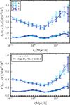Fig. 1. Correlation functions, rpwg+ (top) and $r^2{\stackrel{\sim }{\xi }}_{\mathrm{g}+,2}$ (bottom), in TNG300 for two shape samples: n★ > 300 (continuous lines) and log(M★ h/M⊙) > 10.5 (dashed lines). The shapes are projected over the x (light blue), y (medium blue), and z (dark blue) axes and measured using the simple inertia tensor.

Figure 1 shows that the three different projections along the x, y and z axes are consistent with each other, although at large scales (r_(p) ≳ 8 Mpc/h) the data points become noisy due to lack of galaxy pairs and sometimes only the error bars overlap, indicating the errors may be underestimated. The agreement between the signals confirms the expected behaviour that there should be no significant difference between the various line-of-sight projections and that the common choice of projecting onto the xy plane is arbitrary. Furthermore, it can be observed that within the same simulation, the error bars on the quadrupoles are smaller compared to those on w_g+, and even though the signal amplitude is lower too, the mean S/N is higher as can be seen in Sect. 5.3. This highlights the benefits of using the quadrupole as potential alternative estimators for the density-shape correlation, as suggested by Singh et al. (2024).

Our choice of Π_max = 20 Mpc/h for w_g+ means that the shapes of the correlation functions are very similar between w_g+ and the quadrupole up to separations of 20 Mpc/h (provided we take out the main r_(p)-dependence). Choosing a larger value for Π_max, adds more noise at large scales to w_g+, as can be seen in Fig. A.1.

Comparing the mass cuts, we observe that the high mass sample indeed produces a much larger signal amplitude for both w_g+ and ${\stackrel{\sim }{\xi }}_{\mathrm{g}+,2}$. We also see that the error bars for the high mass cut are larger, due to the smaller sample size. As shown in Sect. 5.3, this stronger signal does not lead to a higher S/N, because both the signal and noise increase by a similar factor.

These signals have also been measured for shapes measured by the reduced inertia tensor. As this produces rounder shapes, the amplitudes of those signals are much lower. However, the comparison between the different cuts and projections is very similar to Fig. 1. Furthermore, IA correlation functions have been measured in TNG100 for both mass cuts and shape types. Therein, the correlations are much noisier due to the smaller box size, which also leads to a decreased signal strength. Barring that, the signals show the same main conclusions as for TNG300. The S/N values for TNG100 are shown in Appendix C.

5.2. Combined covariance matrix

Figure 2 illustrates the normalised combined covariance matrix, as defined in Eq. (13) and normalised by Eq. (17), for the shape sample defined by n_★ > 300 for w_g+ (top panel) and ${\stackrel{\sim }{\xi }}_{\mathrm{g}+,2}$ (bottom panel).

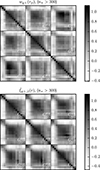Fig. 2. Normalised combined covariance matrices for wg+ (top panel) and ${\stackrel{\sim }{\xi }}_{\mathrm{g}+,2}$ (bottom panel) for the n★ > 300 shape sample. Darker colours indicate higher values. Each block of the combined covariance matrix is labelled according to the definitions in Sect. 3.4.

For both w_g+ and the quadrupole, the combined covariance matrix exhibits the expected symmetry along the diagonal of the auto-correlation blocks (e.g. C^xx). Comparing the w_g+ and the quadrupole covariance matrices, we see notable differences between the two. The quadrupole (bottom panel) shows a similar structure in all the auto-correlation and cross-correlation blocks: a high value diagonal; low values for cross-terms with small scales; high values for intermediate scales, r ≳ 0.5 Mpc/h, that gradually decrease as the scales increase. This basic structure is visible in every block, where naturally the central diagonal (auto-correlation blocks) is highest, as it is set to 1 by definition. For w_g+ (top panel), we see a less coherent structure arise. The cross-correlation (off-diagonal) blocks do not show a clear diagonal and while the ‘middle’ scales have higher values than the cross terms with small or large scales, the normalised values are lower than for the quadrupole; the median value of the ratio between w_g+ and ${\stackrel{\sim }{\xi }}_{\mathrm{g}+,2}$ of all elements ($C_{\mathit{ij}}(w_{\mathrm{g}+})/C_{\mathit{ij}}({\stackrel{\sim }{\xi }}_{\mathrm{g}+,2})$) is ∼0.84. Therefore, it seems that the signals of different projections are less correlated for w_g+ than for the quadrupole.

In Appendix B, where the effects of using 64 jackknife regions (instead of 125) are explored, we see that the normalised values of the covariance matrix are generally lower than in Fig. 2. This indicates either that choosing 125 jackknife regions overestimates the covariance, or that choosing 64 jackknife regions underestimates the covariance. We have opted for 125 jackknife regions in this work because these covariance matrices are more stable (see Appendix B). Furthermore, Appendix E explores the effect of averaging the diagonal and off-diagonal covariance blocks, which should be equal, given that there is no preferred line-of-sight direction in a large enough box. This reduces the noise of the covariance estimate, but erases the influence of the variation in the large scale structure that arises due to the limited box size.

5.3. Signal-to-noise ratio comparison

We compare the S/Ns of using one or more projections, defined in Sect. 3.5. A higher S/N indicates a more robust detection of the intrinsic alignment signal against the background noise.

We calculate the S/N for three cases: once for each individual projection {x, y, z}, S/N (1); three times for a combination of two projections, S/N (2) {(x, y),(y, z),(x, z)}; and once using the combined covariance matrix and concatenated data vector from all three projections, S/N (3). If the signals from the different projections {x, y, z} are completely uncorrelated, the maximum improvement in S/N that we can expect by combining the three projections is a factor of $\sqrt{3}\approx 1.73$ compared to using any individual projection alone, or $\sqrt{2}\approx 1.41$ for two projections. The results are shown in Fig. 3 and Table 1.

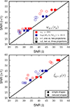Fig. 3. S/Ns for the wg+ (top) and ${\stackrel{\sim }{\xi }}_{\mathrm{g}+,2}$ (bottom) of combining one vs. two (unfilled) and two vs. three (filled) projections. The colours of the markers correspond to the different shape samples: n★ > 300 is red and log(M★h/M⊙) > 10.5 is blue. Shapes measured using the simple, reduced inertia tensor are depicted by circles, crosses, respectively. The black line denotes the boundary marking where both S/N values are equal.

Figure 3 shows the improvement in S/N when one extra projection is added for w_g+ (top panel) and ${\stackrel{\sim }{\xi }}_{\mathrm{g}+,2}$ (bottom panel). In other words, the unfilled markers show the S/N for one projection on the horizontal axis versus two projections on the vertical axis, whereas the filled markers show two versus three projections, respectively. The colours denote the shape sample that is used: red for n_★ > 300 and blue for log(M_★h/M_⊙) > 10.5. Furthermore, the circles represent the measurement of the shapes using the simple inertia tensor (Eq. (1)) and the crosses, the reduced inertia tensor (Eq. (2)). The black line is plotted at S/N(i) = S/N(i + 1). Therefore, an improvement in S/N is shown by the marker residing in the top left half of the plot. For the one versus two projection markers (unfilled), the combinations {x, (x, y)}, {y, (y, z)} and {z, (x, z)} are shown.

For both w_g+ and ${\stackrel{\sim }{\xi }}_{\mathrm{g}+,2}$, almost all cases show a clear improvement in S/N when the information of an extra projection is added. For clarity, Table 1 has been added, which shows the gain in S/N, averaged over the three combinations that are shown individually in Fig. 3 for each choice in shape sample, statistic and shape type. Together, Fig. 3 and Table 1 reveal that for all our cuts and shape types, we can expect a gain in S/N when combining two or three projections, where adding the third projection to two projections will result in less gain than adding a second projection to one projection (the filled markers are closer to the line than the unfilled ones in Fig. 3). The gain in S/N and the S/N values themselves are similar for both mass cuts, despite the high mass sample having a much higher signal amplitude. Furthermore, the gain in S/N for the reduced shapes is generally higher than the gain in S/N for the simple shapes. Finally, the gain in S/N is higher for w_g+ than for the quadrupole, although the quadrupole still has a larger S/N in all cases.

One possible reason for these differences in gain is the influence of the covariance resolution criterion in the S/N calculation as described in Sect. 3.5. The number of terms included in the S/N is always higher for w_g+ than for ${\stackrel{\sim }{\xi }}_{\mathrm{g}+,2}$ and higher for reduced shapes than for simple shapes. As each term included into the S/N increases the S/N, more terms added will increase the chances in S/N gain when projections are combined.

5.4. Model and fit

In this section we present the results of fitting the NLA model to w_g+ and ${\stackrel{\sim }{\xi }}_{\mathrm{g}+,2}$. First, we assess the quality of the fit and then investigate the improvement of S/N when combining projections, analogous to Sect. 5.3. However, in this section we restrict the scales to r_(p) > 6 Mpc/h, only investigating the S/N obtained with common NLA modelling choices. Therefore, the results shown here serve two purposes, first, to investigate how different scales contribute to the gain in S/N, and second, to examine how the pure gain in S/N propagates into uncertainty of the inferred NLA amplitude.

Figure 4 shows the combined fit along the x-, y- and z-axis (light, medium and dark blue) for w_g+ (top panel) and ${\stackrel{\sim }{\xi }}_{\mathrm{g}+,2}$ (bottom panel) galaxy-shape correlation functions, both for particle number (downward triangle) and mass cut (upward triangle) using the simple inertia tensor definition. The NLA model is fitted in the unshaded region and displayed as solid line for the particle number cut and dashed line for the mass cut. It must be noted that the individual points in Fig. 4 are highly correlated, not only between different projection directions, but also between r_(p) bins due to mode mixing. However, we can judge the goodness of fit with the reduced χ_red² shown in Table 2. It ranges from 0.47 to 1.59 and is generally lower for w_g+, possibly indicating slightly over-predicted error bars, but nevertheless an acceptable fit.

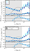Fig. 4. Correlation functions, rpwg+ (top) and $r^2{\stackrel{\sim }{\xi }}_{\mathrm{g}+,2}$ (bottom) in TNG300 for two shape samples: n★ > 300 (downward triangle) and log(M★ h/M⊙) > 10.5 (upward triangle). The shapes are projected over the x (light blue), y (medium blue) and z (dark blue) axes and measured using the simple inertia tensor, whereas the joint NLA fit is shown as a solid (dashed) line for the cut in n★ (M★). The second panel in both plots shows the fit residual for the y-projection. Grey regions indicate excluded regions for the fit. Note: the data points are slightly horizontally displaced for easier readability.

The fitted amplitudes for all available measurements are displayed in Table 2 as well. We find a consistent ∼25% difference in inferred A_IAb_g between w_g+ and ${\stackrel{\sim }{\xi }}_{\mathrm{g}+,2}$. We believe that this is caused by both methods probing different scales and further discuss this in Appendix F. Still, the inferred A_IAb_g are internally consistent for the individual projection directions, enabling us to investigate the gain in S/N in a similar way to what is described in the previous sections. In this case, we can define the S/N as the fraction between fitted amplitude (A_IAb_g) and associated error (σ(A_IAb_g)) obtained by minimising the χ²-statistic defined in Eq. (25):

$$\begin{array}{c}\hfill \mathrm{S}/\mathrm{N}(A_{\mathrm{IA}}{b}_{\mathrm{g}}):=\frac{A_{\mathrm{IA}}{b}_{\mathrm{g}}}{\sigma (A_{\mathrm{IA}}{b}_{\mathrm{g}})}·\end{array}$$(26)

The increase in S/N by adding additional projections is shown in Fig. 5. We show improvement in S/N(A_AIb_g) as a function of added projections for particle number cut (mass cut) in red (blue), both for simple and reduced inertia tensor shapes (points and crosses, respectively). Unfilled markers indicate the improvement when going from one to two projections, and filled markers when going from two to three projections. Again, the points above the one-to-one line indicate a gain in S/N when adding additional projections. As before, increasing the number of projections used increases the S/N. The improvement is further quantified in Table 3 where we average over the gain when adding an additional projection. Note that with the definition from Eq. (26), it is no longer necessarily true that the increase in S/N is bounded by the factors $\sqrt{2}$ or $\sqrt{3}$ when adding one or two projections, respectively. We discuss this further below.

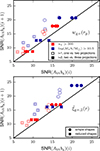Fig. 5. Same as Fig. 3, but for the S/N defined in Eq. (26) obtained from the non-linear alignment model fit.

Similarly to Sect. 5.3, the S/N increases in almost all cases when adding more projections, whereas the gain is larger when adding a second projection than a third. A notable exceptions is w_g+ for reduced shapes using the particle number cut, where the S/N decreases slightly on average when adding a third projection. We believe this to be cause by the resolution condition (Eq. (19)): The error on the correlation function is larger for the higher r_p we consider in this chapter. Therefore, adding highly correlated points means proportionally also adding more noise that can lead to removing more values after the SVD; see also Appendix C. This problem is unique to noisy covariance matrix estimators that might not have full rank and require the aforementioned treatment.

When considering the full data vector in Sect. 5.3, w_g+ benefits more on average than ${\stackrel{\sim }{\xi }}_{\mathrm{g}+}$ when adding additional projections. Here, the reverse seems to be the case. A possible reason for the difference is the additional coupling of the goodness of fit into the S/N consideration. Mathematically, the only difference between the χ² and the actual S/N is the input model (see Eqs. (22) and (25). Since the covariance of the fit parameter is closely related to the Hessian of χ², (Cramér 1946; Rao 1945), we expect that improvements in the goodness-of-fit will propagate into the actual S/N(A_AIb_g). This might further explain why the gain slightly exceeds the theoretical threshold of $\sqrt{2}$ for the reduced-shape ${\stackrel{\sim }{\xi }}_{\mathrm{g}+}$ measurements in the high mass cut case, in particular with a noisy jackknife covariance matrix that is limited by the box size. The question arises whether this behaviour remains with a more robust covariance that is obtained by analytical means. However, this question is outside the scope of this work and can be tackled in future projects.

Even though the fitted NLA amplitudes are affected by a limited scale range and box size, the S/N shows improvement when combining information of multiple projections in the simulation box. The improvement decreasing when going from two to three projections versus from one to two is further in agreement with the results presented in Sect. 5.3. This again solidifies the advantages of this method for obtaining the maximum amount of available information for computationally expensive and extensive hydrodynamical cosmological simulations.

6. Discussion

In this work, we have studied the intrinsic alignments of galaxies in hydrodynamic simulation using the projected shape correlation function, w_g+, and the quadrupole, ${\stackrel{\sim }{\xi }}_{\mathrm{g}+,2}$. Combining the information of the measurements of the intrinsic alignment signals when projected over the three different axis in a simulation box (x, y, z), has led to an increased S/N in most studied cases. Combining two or three projections leads to a gain in S/N for both w_g+ and ${\stackrel{\sim }{\xi }}_{\mathrm{g}+,2}$, for shapes measured with the simple or reduced inertia tensor and for two distinct shape samples defined by n_★ > 300 and log(M_★ h/M_⊙) > 10.5 (see Fig. 3 and Table 1). This gain in S/N when adding a second projection is robust under a change in Π_max, number of jackknife regions used in the covariance estimate and simulation box size (see Appendices A, B and C). There is additional gain in S/N when adding a third projection in the fiducial case, but this is sensitive to the aforementioned changes explored in Appendices A, B, C, and E, where the gain is more marginal.

Compared to the quadrupole measured in Singh et al. (2024) for TNG100, the ${\stackrel{\sim }{\xi }}_{\mathrm{g}+,2}$ signals we measured in TNG300 and TNG100 are very comparable in amplitude and shape. An in-depth comparison is difficult as the scales probed by Singh et al. (2024) only partially overlap with those we chose to study. Regarding the w_g+ signal, we find a good qualitative agreement with previous work. Very similar signal shapes and amplitudes have been measured by e.g. Samuroff et al. (2021) in TNG300, Illustris and MassiveBlack-II; Chisari et al. (2015) in HorizonAGN and Delgado et al. (2023) in MillenniumTNG740, where discrepancies between them mainly arise from differences in galaxy sample selections and the box sizes of the simulations used. In Fig. 1 we see the effect that sample selection can have on the amplitude of the signal and a similar comparison for TNG100 shows that the same sample definitions will lead to lower signal amplitudes in TNG100 when compared to TNG300.

In agreement with (Singh et al. 2024), comparing the S/Ns of w_g+ to ${\stackrel{\sim }{\xi }}_{\mathrm{g}+,2}$, the latter consistently yields a higher S/N for all considered samples, as shown in Fig. 3. However, this is strongly dependent on the chosen value of Π_max, as discussed in Appendix A. When comparing this to the gain in S/N created by adding the information of multiple projections we see that only when comparing the S/N using one projection for the quadrupole to the S/N using three projections for w_g+, do we find that the S/N(3) for w_g+ is larger than S/N(1) for ${\stackrel{\sim }{\xi }}_{\mathrm{g}+,2}$ for a samples using reduced shapes, whereas adding a second projection to w_g+ (S/N(2)) already produces are higher S/N than ${\stackrel{\sim }{\xi }}_{\mathrm{g}+,2}$ with one projection, represented by S/N(1), for simple shapes. This makes the multipole-based estimator a very promising avenue to extract information about IA models from measurements in a more optimal way, especially when multiple projections are combined. Future works could explore the effectiveness of combining multiple projections for other estimators, e.g. the one proposed by Lamman et al. (2025), which will likely show similar gains in S/N.

In this work, we model the correlation functions with the non-linear alignment model (Catelan et al. 2001), that has been shown to be a good model fit for observational galaxy alignment measurements (Singh et al. 2015; Dark Energy Survey and Kilo-Degree Survey Collaboration 2023). Even though the χ_red² indicate good fits for ${\stackrel{\sim }{\xi }}_{\mathrm{g}+,2}$ and w_g+, we detect a consistent mis-match of ∼25% between alignment amplitude obtained from the two different estimators. In Appendix F we show that this can be attributed to a different sensitivity of the estimators to nonlinear physics. Hence, we expect that not only more conservative scale cuts are necessary for ${\stackrel{\sim }{\xi }}_{\mathrm{g}+,2}$ for reliable modelling, but choices of Π_max will influence their comparability as well. More stringent restrictions on reliable scales reduce the total S/N of the measurement, possibly diminishing one of the main advantages of using multipole expanded correlation functions instead of projected ones. We conclude that, even though ${\stackrel{\sim }{\xi }}_{\mathrm{g}+,2}$ has a higher S/N in measurement and corresponding alignment amplitude, better modelling is necessary to exploit the higher S/N of the measurement. The obtained fitted amplitudes are comparable in magnitude to Singh et al. (2024) who carried out a similar analysis on TNG100 data. However, the exact amplitude is highly dependent on galaxy definition and inertia tensor choice, as we demonstrated throughout this work.

Nevertheless, the obtained alignment amplitudes A_IAb_g are consistent between the different projection directions, both for individual and combined projections. By normalising the fitted amplitude with the modelling uncertainty, we obtain S/N(A_AIb_g). Similarly to the measurement S/N, we obtain a clear improvement when adding combining projections that subsequently decreases with number of projections. It must be noted that the improvement exceeds the theoretical limit $\sqrt{N}$ in the case of reduced shapes with mass cut for ${\stackrel{\sim }{\xi }}_{\mathrm{g}+,2}$. The average improvement when going from one to two projections is slightly higher than $\sqrt{2}$ for this specific measurement. Furthermore, the S/N gain is smaller when going from one to three projections than from one to two projections for w_g+ in the reduced inertia tensor sample obtained from the particle number cut. We believe this to be caused by a noisy covariance matrix that propagates into the modelling uncertainty with which we define the S/N(A_AIb_g), in particular since the gain exceeds the threshold for only one of the eight considered cases. This can be further investigated in the future by using more stable covariance matrix estimators.

While the jackknife resampling technique is widely used for estimating covariance matrices, particularly in IA studies, it has known limitations. In the case of this work, it appears that our combined covariance matrix is only stable enough to provide robust results when using the resolution condition, described in Sect. 3.5. In the case of 125 jackknife regions, we filter out 0–6 (mean: 2) elements in the S/N calculation for one projection, 5–13 (7) for two and 9–17 (11) for three, where more elements are filtered out for the quadrupole than w_g+ and simple than reduced shapes; and none of the elements that are used in fitting are filtered out. For 64 jackknife regions, in each case, more elements are filtered out than for 125 jackknife regions. Furthermore, we have seen in Appendix B that the results are sensitive to the number of jackknife regions used. To further investigate this, it would be valuable to compare our jackknife covariance matrix to an analytically calculated covariance matrix. This is a complicated task but presents a possibility for future research. Taking the example of Samuroff et al. (2021), they compare their jackknife covariance matrix to an analytically calculated matrix and find that on scales r_p > 6 Mpc/h, the jackknife tends to underestimate the variance of w_g+ by up to ∼25–50 percent for the TNG300 simulation.

Another viable avenue of further research would include being able to predict covariance of the analytical relations between the projected shapes of our measured ellipsoids. While this is outside of the scope of this work, it would provide insights into why we see a gain in information when adding multiple projections.

As many hydrodynamical simulations currently in use will have comparable or larger box sizes than TNG300, we can assume that our results can be used to measure the IA signals with a consistently larger S/N. Using relatively little computing power compared to the amount needed to run larger simulations, we can use the existing hydrodynamical simulations to better constrain modelling priors currently derived from these same simulations.

7. Conclusions

In this work, we have combined the information of shapes of galaxies projected over multiple axes, while taking their covariance into account, in hydrodynamical simulation TNG300. We show that a consistent and robust gain in S/N can be obtained for both w_g+ and ${\stackrel{\sim }{\xi }}_{\mathrm{g}+,2}$ by combining multiple projections. Below, the main conclusions are summarised.

1. Combining the information of more than one projection, the S/Ns of both w_g+ and ${\stackrel{\sim }{\xi }}_{\mathrm{g}+,2}$ are consistently larger than for a single projection (Table 1 and Fig. 3).

2. Adding a second projection leads to a larger gain in S/N than adding a third projection for both w_g+ and ${\stackrel{\sim }{\xi }}_{\mathrm{g}+,2}$ (Table 1 and Fig. 3).

3. The gain in S/N when adding two or three projections is larger for shapes measured with the reduced inertia tensor than with the simple inertia tensor (Table 1 and Fig. 3).

4. Table 1 shows that the gain in S/N for a high mass shape sample (log(M_★ h/M_⊙) > 10.5) is similar to that for all galaxies with resolved shapes (n_★ > 300), where the high mass sample signal has a much higher amplitude (Fig. 1).

5. The S/N of the fitted amplitude obtained from the non-linear alignment model increases when adding projections in almost all cases but shows inconclusive systematic behaviour between estimators and sample selection. This is likely caused by the increased uncertainty on larger scales commonly used for modelling (Table 3 and Fig. 5).

Acknowledgments

We thank Casper Vedder for plenty of useful discussions. This publication is part of the project “A rising tide: Galaxy intrinsic alignments as a new probe of cosmology and galaxy evolution” (with project number VI.Vidi.203.011) of the Talent programme Vidi which is (partly) financed by the Dutch Research Council (NWO). DN and HH acknowledge support from the European Research Council (ERC) under the European Union’s Horizon 2020 research and innovation program with Grant agreement No. 101053992.

References

Appendix A: Π_max

As mentioned in Sect. 3.2, the choice in the integration limit Π_max can have a significant impact on the measurement of w_g+. In order to match the measurements of the quadrupole more closely, which is dependent on the 3D separation between a galaxy pairs, the results in the main body of the text are measured with Π_max = 20Mpc/h, matching the maximum r and r_p values. In order to give so insight into the influence of the choice in Π_max on the results, Fig. A.1 shows r_pw_g+ when measured with Π_max = 102.5Mpc/h, for both shape samples n_★ > 300 (continuous lines) and log(M_★h/M_⊙) > 10.5 (dashed lines) in all three projections x (light blue), y (medium blue) and z (dark blue), similarly to Fig. 1 in the main text.

When comparing Fig. A.1 to the top panel of Fig. 1, we can see that the shape of the correlation functions has changed, mainly for large scales (r_p ≳ 3Mpc/h). The signal shape matches that of the quadrupole (Fig. 1, bottom panel) less closely. Moreover, the signal at these larger scales is much noisier for a larger Π_max, which is apparent in both the larger error bars in Fig. A.1 and the divergence of the different projections.

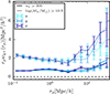Fig. A.1. Correlation function, rpwg+, for Πmax = 102.5Mpc/h, in TNG300 for two shape samples: n★ > 300 (continuous lines) and log(M★h/M⊙) > 10.5 (dashed lines). The shapes are projected over the x (light blue), y (medium blue) and z (dark blue) axes and measured using the simple inertia tensor.

Figure A.2 shows the S/Ns of one versus two (unfilled markers) projections and two versus three (filled) for simple (circles) and reduced (crosses) shapes and for both mass cuts n_★ > 300 (red) and log(M_★h/M_⊙) > 10.5 (blue). The figure is equivalent to the top panel of Fig. 3 in the main text, with the only difference being that here w_g+ was calculated using a Π_max of 102.5Mpc/h. Comparing Fig. A.2 to the top panel of Fig. 3, we can see that a larger Π_max results in much lower S/Ns for w_g+ because of the noisier data vector. Looking at both Fig. A.2 and Table A.1, we see that the rest of the conclusions from the main text remain valid: adding a second projection has a larger gain than the third, although each projection added increases the S/N; the gain in S/N is higher for reduced shapes than simple ones and the gains are comparable between the mass cuts. However, comparing Table A.1 to Table 1, we see that the gains in S/N when adding projections are higher for a larger value of Π_max, even though the S/Ns themselves remain lower.

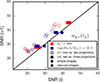Fig. A.2. S/Ns for the wg+ of combining one vs two (unfilled) and two vs three (filled) projections. The colours of the markers correspond to the different shape samples: n★ > 300 is red and log(M★h/M⊙) > 10.5 is blue. Shapes measured using the simple, reduced inertia tensor are depicted by circles, crosses, respectively. The black line denotes the boundary for which both S/Ns are equal. In this figure, Πmax = 102.5Mpc/h, instead of 20Mpc/h as it is in Fig. 3.

Appendix B: Jackknife regions

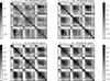Fig. B.1. Normalised combined covariance matrices for wg+ (top) and ${\stackrel{\sim }{\xi }}_{\mathrm{g}+,2}$ (bottom) for the n★ > 300 shape sample, using 64 jackknife samples (left) or 125 jackknife regions (right). Darker colours indicate higher values. Each block of the combined covariance matrix is labelled according to the definitions in Sect. 3.4. The right side of the figure is equal to Fig. 2.

The chosen number of jackknife regions can potentially have a large impact on the S/Ns obtained, as the over- or underestimation of the covariance can lead to very different S/Ns. Furthermore, if the choice in the number of jackknife regions leads to instability in the covariance, the resulting S/Ns can become unreliable and even nonsensical. Especially for the combination of three projections, the covariance matrix is sensitive to these instabilities, due to the high number of strongly correlated elements. Therefore, we have studied two options for the number of jackknife regions: 125 and 64, settling on 125 for TNG300, which is used in the main body of the text as it seems to be the most stable.

The superior stability of 125 jackknife regions versus 64 can be substantiated in two ways. First, when applying the covariance resolution condition, as described in Sect. 3.5, we see that in the case of 125 jackknife regions, systematically, more eigenvalues of the SVD pass the resolution criterium and therefore contribute to the S/N than for 64 jackknife regions. Second, we expect the addition of each term to result in a monotonic increase in the S/N. While this is not true in every case, we see that it is true for many more of the cases using 125 jackknife regions than 64 regions. Combined with the invertability of the matrices and the reasonable values obtained for the S/Ns, the choice of 125 jackknife regions seems to make the most sense.

In this appendix the normalised combined covariance matrices for w_g+ and ${\stackrel{\sim }{\xi }}_{\mathrm{g}+,2}$ are shown for 64 jackknife regions (4³, left side) and 125 jackknife regions (5³, right side) in Fig. B.1, where the right side is is analogous to Fig. 2 and has been added for comparison.

As mentioned in Sect. 5.2, the values of the normalised combined covariance are lower when using 64 jackknife regions than 125, especially for w_g+. This can be seen in Fig. B.1, when comparing the left and right side of the figure: the right side is generally darker, indicating higher values. When taking the median of the ratios between 64 and 125 regions for all elements, we find that this is ∼0.95 for w_g+ and ∼1.0 for ${\stackrel{\sim }{\xi }}_{\mathrm{g}+,2}$. Barring that, the same basic structures arise in both versions of the covariance, consolidating the trust in the measurement accuracy in general.

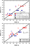Fig. B.2. S/Ns for the wg+ (top) and ${\stackrel{\sim }{\xi }}_{\mathrm{g}+,2}$ (bottom) of combining one versus two (unfilled) and two versus three (filled) projections in TNG300 for 64 jack-knife regions. The colours of the markers correspond to the different shape samples: n★ > 300 is red and log(M★h/M⊙) > 10.5 is blue. Shapes measured using the simple, reduced inertia tensor are depicted by circles, crosses, respectively. The black line denotes the boundary for which both S/Ns are equal.

The impact of the number of jackknife regions on the S/N gains can be seen in Fig. B.2 and Table B.1. While decreasing the number of jackknife regions alters the S/N compared to Fig. 3 and Table 1, the main conclusions presented in Sect. 5.3 remain valid. Adding the second projections increases the S/N in nearly all cases, and in some, adding a third projection also adds additional S/N. The S/N gain also seems to be higher for reduced shapes than for the simple ones and is once again comparable for both shape samples (mass cuts). Furthermore, the difference gain in w_g+ and ${\stackrel{\sim }{\xi }}_{\mathrm{g}+,2}$ seen in Sect. 5.3 is also still there.

The only qualitative difference between using 64 or 125 jackknife regions for the S/N gain, is that when using 64 regions, there are many cases (mostly for simple shapes) where adding a third projection is decreasing the S/N instead of increasing it, leading to sub-one ratios in Table B.1.

In conclusion, the main trends and conclusions seem trustworthy, although there is some sensitivity of the results to the number of jackknife regions. This mostly shows the limitations of the jackknife method for covariance estimation, even when correcting for biases. Ideally, we would use multiple independent realisations of the simulation to estimate the covariance, but with the cost of running hydrodynamical simulations, this is not feasible.

Appendix C: Box size and resolution

This appendix explores the influence of the simulation box size and resolution on the gain in S/N when adding the information of two or three projections to the intrinsic alignment correlation functions. These effects are explored together by doing the same measurements as in the rest of the paper for TNG100-1 instead of TNG300-1, which has a smaller box size (L_box = 75cMpc/h and a higher resolution (1820³ dark matter particles of mass m_DM = 7.5 × 10⁶M_⊙).

Figure C.1 and Table C.1 are the counterparts of Fig. 3 and Table 1, showing the gain in S/N when adding projections in TNG100 for the two shape samples and shape types in both w_g+ (top panel) and ${\stackrel{\sim }{\xi }}_{g+,2}$ (bottom). As the box size of TNG100 is smaller, we opted to use 64 jackknife regions to measure the covariance and used 15 r_(p) bins between 0.1 Mpc/h and 20 Mpc/h. Figure C.1, shows that while the markers lie much closer to the line than in Fig. 3 (for TNG300), the unfilled markers generally still lie in the top left half of the figure, indicating a gain in S/N when adding a second projection (going from one to two projections: unfilled markers; from two to three: filled). The figure axes limits announce that we are in a difference S/N regime: the S/Ns in TNG100 are much lower than in TNG300. This is to be expected, as the box size is much smaller and the measurements are therefore noisier. Adding the information presented in Table C.1, we see that our main conclusions, exhibited in Sect. 5.3, hold. As in TNG300, in TNG100 the gains in S/N are larger when adding the second to the first projection than adding the third to the second (if there is any gain in when adding the third). Also, the gains in S/N when adding projections for the reduced shapes (crosses) are higher than those for the simple shapes (circles) more often than not. Furthermore, the gains in S/N when adding projections (and the S/N values themselves) for the shape samples defined by n_★ > 300 (red) and log(M_★h/M_⊙) > 10.5 (blue) are comparable.

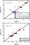Fig. C.1. S/Ns for the wg+ (top) and ${\stackrel{\sim }{\xi }}_{g+,2}$ (bottom) of combining one versus two (unfilled) and two versus three (filled) projections in TNG100. The colours of the markers correspond to the different shape samples: n★ > 300 is red and log(M★h/M⊙) > 10.5 is blue. Shapes measured using the simple, reduced inertia tensor are depicted by circles, crosses, respectively. The black line denotes the boundary for which both S/Ns are equal.

In conclusion, the main conclusions drawn in Sect. 5.3 are not severely impacted by simulation box size and resolution. While individual cases will differ, the trends are robust. Combining the results in this appendix, to those in Appendices A and B we can state that when the measurement becomes noisier (due to e.g. higher Π_max, fewer jackknife regions or smaller box size), the impact of adding a second projection is increased, while the impact of adding a third projection is mitigated by the addition of extra noise.

Appendix D: Motivation of the resolution condition in given by Eq. (19)

We first remind ourselves that the Jackknife covariance estimate is given by Eq. (10). Here, we define the difference between Jackknife per-region estimate and mean as ${\mathrm{\Delta }}_i^{[k]}:={\psi }_i^k-{\overline{\psi }}_i$, with ${\overline{\psi }}_i$ from Eq. (11). Therefore, the Jackknife covariance estimate becomes

$$\begin{array}{c}\hfill {\widehat{C}}_{\mathit{ij}}=\frac{N_{\mathrm{sub}}-1}{N_{\mathrm{sub}}}{\displaystyle \sum _{k=1}^{N_{\mathrm{sub}}}}{\mathrm{\Delta }}_i^{[k]}{\mathrm{\Delta }}_j^{[k]}.\end{array}$$(D.1)

We stress that in this section ${\widehat{C}}_{\mathit{ij}}$ denotes the covariance estimator and not the rescaled covariance matrix described in Sect. 3.5. The individual ${\left\{{\{{\mathrm{\Delta }}_i^{[k]}\}}_{i=1\dots p}\right\}}_{k=1\dots N_{\mathrm{sub}}}$ are matrix elements for the p × N_sub random matrix, where N_sub is the number of Jackknife regions and p the number of used r_(p) bins, i.e. measurement points. Assuming the points to be drawn from a p-dimensional Gaussian 𝒩(0, Σ′) with scale matrix Σ′, Eq. (D.1) is of the same functional form as the Wishart-distributed random scatter matrix (Wishart 1928; Gupta & Nagar 2000)

$$\begin{array}{c}\hfill {\mathcal{S}}_{\mathit{ij}}={\displaystyle \sum _{k=1}^N}{\mathrm{\Delta }}_i^{[k]}{\mathrm{\Delta }}_j^{[k]}.\end{array}$$(D.2)

Denoting Σ as the true covariance, the variance of ${\widehat{C}}_{\mathit{ij}}$ then directly follows from the Wishart distribution using ν = N_sub − 1 degrees of freedom and the scale matrix Σ′ = Σ/(N_sub − 1) Mohammad & Percival (2022) as¹²

$$\begin{array}{cc}\hfill \mathrm{Var}({\widehat{C}}_{\mathit{ij}})& =\frac{N_{\mathrm{sub}}-1}{N_{\mathrm{sub}}}\nu ({({\mathrm{\Sigma }}_{\mathit{ij}}^{\prime })}^2+{\mathrm{\Sigma }}_{\mathit{ii}}^{\prime }{\mathrm{\Sigma }}_{\mathit{ij}}^{\prime })\hfill \\ \hfill & =\frac{1}{N_{\mathrm{sub}}}({({\mathrm{\Sigma }}_{\mathit{ij}})}^2+{\mathrm{\Sigma }}_{\mathit{ii}}{\mathrm{\Sigma }}_{\mathit{ij}}).\hfill \end{array}$$(D.3)

We note that we would obtain the expression given in Gaztañaga & Scoccimarro (2005), $\mathrm{\Delta }{C}_{\mathit{ij}}\simeq \sqrt{\frac{2}{N_{\mathrm{sub}}}}$, by taking the limiting case of i = j and |Σ_ij|≃𝒪(1). The latter holds if we perform the rescaling as specified in Eq. (17). The former provides an upper bound under the reasonable assumption that the off-diagonals of the covariance matrix are smaller than the diagonal entries.

In the case of a positive-semidefinit real matrix (e.g. a covariance), the SVD is given by

$$\begin{array}{c}\hfill {\widehat{\mathit{C}}\mathbf{=}\mathit{U}}^{\mathrm{T}}\mathit{D}\mathit{U}\mathrm{with}{\mathit{U}}^{\mathrm{T}}\mathit{U}\mathbf{=}\mathit{I}.\end{array}$$(D.4)

Thus, we can translate the bound on ΔC_ij to a cut for eigenvalues after SVD by splitting the estimated covariance into a signal and noise term

$$\begin{array}{cc}\hfill \widehat{\mathit{C}}& =\mathbf{\Sigma }+\mathit{N}={\widehat{\mathit{U}}}^{\mathrm{T}}\widehat{\mathit{D}}\widehat{\mathit{U}}\hfill \\ \hfill ⟹\widehat{\mathit{D}}& ={\widehat{\mathit{U}}\mathbf{\Sigma }\widehat{\mathit{U}}}^{\mathrm{T}}+{\widehat{\mathit{U}}\mathit{N}\widehat{\mathit{U}}}^{\mathrm{T}}\simeq \mathit{D}+{\widehat{\mathit{U}}\mathit{N}\widehat{\mathit{U}}}^{\mathrm{T}}.\hfill \end{array}$$(D.5)

For the individual SVD eigenvalues, this which yields ${\widehat{\lambda }}_i^2\simeq {\lambda }_i^2+{\widehat{U}}_i\mathit{N}{\widehat{U}}_i^{\mathrm{T}}.$ The expected noise contribution is then

$$\begin{array}{cc}\hfill \mathrm{Var}({\widehat{U}}_i\mathit{N}{\widehat{U}}_i^{\mathrm{T}})& =\mathrm{Var}\left({\displaystyle \sum _{j,k}}{\widehat{U}}_{\mathit{ij}}{N}_{\mathit{jk}}{\widehat{U}}_{\mathit{ki}}\right)\hfill \\ \hfill & ={\displaystyle \sum _{j,k}}{\widehat{U}}_{\mathit{ij}}\mathrm{Var}(N_{\mathit{jk}}){\widehat{U}}_{\mathit{ki}}\hfill \\ \hfill & ={\displaystyle \sum _{j,k}}{\widehat{U}}_{\mathit{ij}}{(\mathrm{\Delta }{C}_{\mathit{jk}})}^2{\widehat{U}}_{\mathit{ki}}\hfill \\ \hfill & \simeq \frac{2}{N_{\mathrm{sub}}}{\displaystyle \sum _{\mathit{jk}}}{\widehat{U}}_{\mathit{ij}}{\widehat{U}}_{\mathit{ki}}=\frac{2}{N_{\mathrm{sub}}},\hfill \end{array}$$(D.6)

where we used the orthogonality of $\widehat{\mathit{U}}$. Therefore, ${\sigma }_i\simeq \sqrt{\frac{2}{N_{\mathrm{sub}}}}$ and we expect singular values ${\widehat{\lambda }}_i^2<\sqrt{\frac{2}{N_{\mathrm{sub}}}}$ to be dominated by noise.

Appendix E: Averaged covariance

The full covariance matrix containing all three projections (Sect. 5.2, Fig. 2) shows unexpected discrepancies between the off-diagonal blocks and the diagonal blocks, which should be equal in a perfect world. For a large enough simulation box, we expect there to be no preferred line-of-sight direction, which means that $C_{\mathit{ij}}^{\mathit{xx}}=C_{\mathit{ij}}^{\mathit{yy}}=C_{\mathit{ij}}^{\mathit{zz}}$ and $C_{\mathit{ij}}^{\mathit{xy}}=C_{\mathit{ij}}^{\mathit{xy}}=C_{\mathit{ij}}^{\mathit{yz}}$. The current discrepancies can be attributed to the noisiness of the jackknife covariance estimator and the influence of variations in the large scale structure due to the limited box size. Averaging the diagonal blocks and the off-diagonal blocks, and using this averaged covariance matrix to calculate the S/Ns, gives a lower bound to the S/N gain. This procedure produces a lower bound because the differences in the large scale structure between projections are ignored, which should be taken into account, as they are non-trivial in small simulation boxes.

Figure E.1 shows the S/Ns of one versus two (unfilled markers) and two versus three (filled) for simple (circles) and reduced (crosses) shapes for n_★ > 300 (red) and log(M_★h/M_⊙) > 10.5 (blue) for both w_g+ (top) and ${\stackrel{\sim }{\xi }}_{\mathrm{g}+,2}$ (bottom). Comparing Fig. E.1 to Fig. 3, we see that the gains are slightly lower, but still above unity (black line) in most cases. Table E.1 presents the S/N gains in all cases mentioned previously. Comparing Table E.1 to Table 1, we see that the S/N gains are indeed slightly lower when averaging the covariance blocks, but they are still consistently above 1.0 when increasing the number of projections from 1 to 3 or 1 to 2. These gains are high enough to be considered robust, as even this lower bound scenario produces > 1 S/N ratios. Adding a third projection does not consistently add S/N, as we have already seen in other appendices.

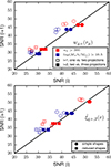Fig. E.1. S/Ns for the wg+ (top) and ${\stackrel{\sim }{\xi }}_{\mathrm{g}+,2}$ (bottom) of combining one vs two (unfilled) and two vs three (filled) projections in TNG300 using the averaged covariance for two and three projections. The colours of the markers correspond to the different shape samples: n★ > 300 is red and log(M★h/M⊙) > 10.5 is blue. Shapes measured using the simple, reduced inertia tensor are depicted by circles, crosses, respectively. The black line denotes the boundary for which both S/Ns are equal.

Appendix F: Fitted amplitude difference between multipole expanded and projected correlation function

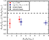Fig. F.1. Fraction of AIAbg obtained from ${\stackrel{\sim }{\xi }}_{\mathrm{g}+,2}$ over AIAbg obtained from wg+ as a function of the AIAbg obtained from wg+ using a Πmax = 20 Mpc/h, depicted in red (blue) for the particle number (mass) cut, and as circles (crosses) for shapes obtained with the simple (reduced) intertia tensor. We show only the case of the joint amplitude across all three axes, since they are fully consistent with the amplitude of the individual axes.

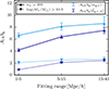Fig. F.2. Evolution of NLA AIAbg when fitting within different scale ranges, shown for particle number and mass cut with upward triangles and solid lines, and downward triangles and dashed lines, respectively. NLA amplitudes fitted with ${\stackrel{\sim }{\xi }}_{\mathrm{g}+,2}$ are depicted in dark blue and those fitted with wg+ in light blue, including the error bars.

In this section, we investigate the difference between NLA amplitude obtained from multipole and projected correlation functions. In Fig. F.1 we show the ratio of NLA amplitude between ${\stackrel{\sim }{\xi }}_{\mathrm{g}+,2}$ and w_g+ as a function of w_g+ NLA amplitude, for simple (reduced) inertia tensor shapes depicted as circles (crosses), and for the particle number (mass) sample cut in red (blue). The amplitudes from ${\stackrel{\sim }{\xi }}_{\mathrm{g}+,2}$ are consistently lower than those of projections. We believe that the most likely explanation for this is the difference in scale dependence. ${\stackrel{\sim }{\xi }}_{\mathrm{g}+,2}$ are functions of the full 3D distance magnitude, r, while w_g+ are functions of the distance perpendicular to the line of sight r_p ≤ r. The fitting range of r_(p) > 6 Mpc/h was chosen close to the scale at which NLA is known to break down for w_g+ (Tenneti et al. 2015). Hence, we can expect a model bias of ${\stackrel{\sim }{\xi }}_{\mathrm{g}+,2}$ if we fit the same scales. In addition, we employed Π_max = 20 Mpc/h for the main body of the paper, staying close to mildly non-linear scales in line-of-sight direction for w_g+ with the advantage of decreasing shape noise at the same time. However, such constraints are naturally not put on ${\stackrel{\sim }{\xi }}_{\mathrm{g}+,2}$. Therefore, we would expect more similar signals for larger Π_max on large r_(p) since w_g+ and ${\stackrel{\sim }{\xi }}_{\mathrm{g}+,2}$ then start probing similar, linear volumes. To illustrate this effect, we additionally measure the correlations in TNG300 using Π_max = 102.5 Mpc/h up to scales of r_max = 40 Mpc/h. Note that this increases the uncertainty on w_g+, making this an unfit measurement for the main analysis of this work. Nevertheless, we can investigate the influence of a model mis-match by fitting the NLA amplitude in three different scale ranges: 1–5 Mpc/h, 5–15 Mpc/h, and 15–40 Mpc/h.

In Fig. F.2 we show the evolution of the fitted NLA amplitude for ranges of increasingly larger scales for w_g+ and ${\stackrel{\sim }{\xi }}_{\mathrm{g}+,2}$ in light and dark blue, respectively, as well as for particle number cut sample with upward triangle symbols and solid line, and mass cut sample with downward triangle symbol and dashed line. We notice that the NLA fit to multipole expanded correlation functions has, as expected, smaller error bars than the fit to projected correlation functions, but also shows a larger mis-match on small scales as opposed to large scales where the NLA model is known to be reasonable. Correspondingly, for ranges of 15–40 Mpc/h the NLA amplitude is consistent between ${\stackrel{\sim }{\xi }}_{\mathrm{g}+,2}$ and w_g+. This leads us to two conclusions: First, naively transferring the accumulated knowledge from modelling projected correlation functions to modelling multipole expanded correlation function will lead to biased results due to different scale dependent behaviour, and second, the bridge between large-scale models such as NLA and small scale models such as the halo model becomes ever more important when dealing with measurements where intermediate scales carry significant part of information, whether that is in simulation boxes of limited sizes or in real-world applications that increasingly rely on pushing scale cuts for improvement in cosmology inference.

All Tables

All Figures

	Fig. 1. Correlation functions, rpwg+ (top) and $r^2{\stackrel{\sim }{\xi }}_{\mathrm{g}+,2}$ (bottom), in TNG300 for two shape samples: n★ > 300 (continuous lines) and log(M★ h/M⊙) > 10.5 (dashed lines). The shapes are projected over the x (light blue), y (medium blue), and z (dark blue) axes and measured using the simple inertia tensor.
In the text

	Fig. 2. Normalised combined covariance matrices for wg+ (top panel) and ${\stackrel{\sim }{\xi }}_{\mathrm{g}+,2}$ (bottom panel) for the n★ > 300 shape sample. Darker colours indicate higher values. Each block of the combined covariance matrix is labelled according to the definitions in Sect. 3.4.
In the text

Fig. 3. S/Ns for the wg+ (top) and ${\stackrel{\sim }{\xi }}_{\mathrm{g}+,2}$ (bottom) of combining one vs. two (unfilled) and two vs. three (filled) projections. The colours of the markers correspond to the different shape samples: n★ > 300 is red and log(M★h/M⊙) > 10.5 is blue. Shapes measured using the simple, reduced inertia tensor are depicted by circles, crosses, respectively. The black line denotes the boundary marking where both S/N values are equal.

In the text

Fig. 4. Correlation functions, rpwg+ (top) and $r^2{\stackrel{\sim }{\xi }}_{\mathrm{g}+,2}$ (bottom) in TNG300 for two shape samples: n★ > 300 (downward triangle) and log(M★ h/M⊙) > 10.5 (upward triangle). The shapes are projected over the x (light blue), y (medium blue) and z (dark blue) axes and measured using the simple inertia tensor, whereas the joint NLA fit is shown as a solid (dashed) line for the cut in n★ (M★). The second panel in both plots shows the fit residual for the y-projection. Grey regions indicate excluded regions for the fit. Note: the data points are slightly horizontally displaced for easier readability.

In the text

	Fig. 5. Same as Fig. 3, but for the S/N defined in Eq. (26) obtained from the non-linear alignment model fit.
In the text

	Fig. A.1. Correlation function, rpwg+, for Πmax = 102.5Mpc/h, in TNG300 for two shape samples: n★ > 300 (continuous lines) and log(M★h/M⊙) > 10.5 (dashed lines). The shapes are projected over the x (light blue), y (medium blue) and z (dark blue) axes and measured using the simple inertia tensor.
In the text

Fig. A.2. S/Ns for the wg+ of combining one vs two (unfilled) and two vs three (filled) projections. The colours of the markers correspond to the different shape samples: n★ > 300 is red and log(M★h/M⊙) > 10.5 is blue. Shapes measured using the simple, reduced inertia tensor are depicted by circles, crosses, respectively. The black line denotes the boundary for which both S/Ns are equal. In this figure, Πmax = 102.5Mpc/h, instead of 20Mpc/h as it is in Fig. 3.

In the text

Fig. B.1. Normalised combined covariance matrices for wg+ (top) and ${\stackrel{\sim }{\xi }}_{\mathrm{g}+,2}$ (bottom) for the n★ > 300 shape sample, using 64 jackknife samples (left) or 125 jackknife regions (right). Darker colours indicate higher values. Each block of the combined covariance matrix is labelled according to the definitions in Sect. 3.4. The right side of the figure is equal to Fig. 2.

In the text

Fig. B.2. S/Ns for the wg+ (top) and ${\stackrel{\sim }{\xi }}_{\mathrm{g}+,2}$ (bottom) of combining one versus two (unfilled) and two versus three (filled) projections in TNG300 for 64 jack-knife regions. The colours of the markers correspond to the different shape samples: n★ > 300 is red and log(M★h/M⊙) > 10.5 is blue. Shapes measured using the simple, reduced inertia tensor are depicted by circles, crosses, respectively. The black line denotes the boundary for which both S/Ns are equal.

In the text

Fig. C.1. S/Ns for the wg+ (top) and ${\stackrel{\sim }{\xi }}_{g+,2}$ (bottom) of combining one versus two (unfilled) and two versus three (filled) projections in TNG100. The colours of the markers correspond to the different shape samples: n★ > 300 is red and log(M★h/M⊙) > 10.5 is blue. Shapes measured using the simple, reduced inertia tensor are depicted by circles, crosses, respectively. The black line denotes the boundary for which both S/Ns are equal.

In the text

Fig. E.1. S/Ns for the wg+ (top) and ${\stackrel{\sim }{\xi }}_{\mathrm{g}+,2}$ (bottom) of combining one vs two (unfilled) and two vs three (filled) projections in TNG300 using the averaged covariance for two and three projections. The colours of the markers correspond to the different shape samples: n★ > 300 is red and log(M★h/M⊙) > 10.5 is blue. Shapes measured using the simple, reduced inertia tensor are depicted by circles, crosses, respectively. The black line denotes the boundary for which both S/Ns are equal.

In the text

Fig. F.1. Fraction of AIAbg obtained from ${\stackrel{\sim }{\xi }}_{\mathrm{g}+,2}$ over AIAbg obtained from wg+ as a function of the AIAbg obtained from wg+ using a Πmax = 20 Mpc/h, depicted in red (blue) for the particle number (mass) cut, and as circles (crosses) for shapes obtained with the simple (reduced) intertia tensor. We show only the case of the joint amplitude across all three axes, since they are fully consistent with the amplitude of the individual axes.

In the text

	Fig. F.2. Evolution of NLA AIAbg when fitting within different scale ranges, shown for particle number and mass cut with upward triangles and solid lines, and downward triangles and dashed lines, respectively. NLA amplitudes fitted with ${\stackrel{\sim }{\xi }}_{\mathrm{g}+,2}$ are depicted in dark blue and those fitted with wg+ in light blue, including the error bars.
In the text

References

- Abbott, T. M. C., Abdalla, F. B., Allam, S., et al. 2018, ApJS, 239, 18 [Google Scholar]
- Abdalla, E., Abellán, G. F., Aboubrahim, A., et al. 2022, J. High Energy Astrophys., 34, 49 [NASA ADS] [CrossRef] [Google Scholar]
- Aihara, H., Arimoto, N., Armstrong, R., et al. 2018, PASJ, 70, S4 [NASA ADS] [Google Scholar]
- Akitsu, K., Li, Y., & Okumura, T. 2023, Phys. Rev. D, 107, 063531 [Google Scholar]
- Albrecht, A., Bernstein, G., Cahn, R., et al. 2006, Report of the Dark Energy Task Force [Google Scholar]
- Bate, J., Chisari, N. E., Codis, S., et al. 2020, MNRAS, 491, 4057 [Google Scholar]
- Bernstein, G. M., & Jarvis, M. 2002, AJ, 123, 583 [NASA ADS] [CrossRef] [Google Scholar]
- Bhowmick, A. K., Chen, Y., Tenneti, A., Di Matteo, T., & Mandelbaum, R. 2020, MNRAS, 491, 4116 [Google Scholar]
- Biagetti, M., & Orlando, G. 2020, JCAP, 2020, 005 [CrossRef] [Google Scholar]
- Blazek, J., McQuinn, M., & Seljak, U. 2011, JCAP, 2011, 010 [CrossRef] [Google Scholar]
- Bridle, S., & King, L. 2007, New J. Phys., 9, 444 [Google Scholar]
- Catelan, P., Kamionkowski, M., & Blandford, R. D. 2001, MNRAS, 320, L7 [NASA ADS] [CrossRef] [Google Scholar]
- Chisari, N. E., & Dvorkin, C. 2013, JCAP, 2013, 029 [CrossRef] [Google Scholar]
- Chisari, N. E., Dvorkin, C., & Schmidt, F. 2014, Phys. Rev. D, 90, 043527 [Google Scholar]
- Chisari, N., Codis, S., Laigle, C., et al. 2015, MNRAS, 454, 2736 [NASA ADS] [CrossRef] [Google Scholar]
- Chisari, N. E., Alonso, D., Krause, E., et al. 2019, ApJS, 242, 2 [Google Scholar]
- Cramér, H. 1946, Mathematical Methods of Statistics (Princeton University Press), Princeton Math. Ser. [Google Scholar]
- Dalal, R., Li, X., Nicola, A., et al. 2023, Phys. Rev. D, 108, 123519 [CrossRef] [Google Scholar]
- Dark Energy Survey and Kilo-Degree Survey Collaboration (Abbott, T. M. C., et al.) 2023, Open J. Astrophys., 6, 36 [NASA ADS] [Google Scholar]
- de Jong, J. T. A., Verdoes Kleijn, G. A., Kuijken, K. H., & Valentijn, E. A. 2013, Exp. Astron., 35, 25 [Google Scholar]
- Delgado, A. M., Hadzhiyska, B., Bose, S., et al. 2023, MNRAS, 523, 5899 [CrossRef] [Google Scholar]
- Dubois, Y., Pichon, C., Welker, C., et al. 2014, MNRAS, 444, 1453 [Google Scholar]
- Eisenstein, D. J., & Zaldarriaga, M. 2001, ApJ, 546, 2 [Google Scholar]
- Fortuna, M. C., Hoekstra, H., Joachimi, B., et al. 2020, MNRAS, 501, 2983 [Google Scholar]
- Gaztañaga, E., & Scoccimarro, R. 2005, MNRAS, 361, 824 [Google Scholar]
- Genel, S., Vogelsberger, M., Nelson, D., et al. 2013, MNRAS, 435, 1426 [NASA ADS] [CrossRef] [Google Scholar]
- Gupta, A. K., & Nagar, D. K. 2000, Matrix Variate Distributions (Boca Raton, FL: Chapman and Hall/CRC) [Google Scholar]
- Hartlap, J., Simon, P., & Schneider, P. 2006, A&A, 464, 399 [Google Scholar]
- Hearin, A. P., Campbell, D., Tollerud, E., et al. 2017, AJ, 154, 190 [Google Scholar]
- Heymans, C., Tröster, T., Asgari, M., et al. 2021, A&A, 646, A140 [NASA ADS] [CrossRef] [EDP Sciences] [Google Scholar]
- Hirata, C. M., & Seljak, U. 2004, Phys. Rev. D, 70, 063526 [Google Scholar]
- Hirata, C. M., Mandelbaum, R., Ishak, M., et al. 2007, MNRAS, 381, 1197 [NASA ADS] [CrossRef] [Google Scholar]
- Ivezić, Ž., Kahn, S. M., Tyson, J. A., et al. 2019, ApJ, 873, 111 [Google Scholar]
- Jarvis, M., Bernstein, G., & Jain, B. 2004, MNRAS, 352, 338 [Google Scholar]
- Joachimi, B., & Bridle, S. L. 2010, A&A, 523, A1 [NASA ADS] [CrossRef] [EDP Sciences] [Google Scholar]
- Joachimi, B., Mandelbaum, R., Abdalla, F. B., & Bridle, S. L. 2011, A&A, 527, A26 [NASA ADS] [CrossRef] [EDP Sciences] [Google Scholar]
- Joachimi, B., Cacciato, M., Kitching, T. D., et al. 2015, Space Sci. Rev., 193, 1 [Google Scholar]
- Khandai, N., Di Matteo, T., Croft, R., et al. 2015, MNRAS, 450, 1349 [NASA ADS] [CrossRef] [Google Scholar]
- Kiessling, A., Cacciato, M., Joachimi, B., et al. 2015, Space Sci. Rev., 193, 67 [Google Scholar]
- Kilbinger, M. 2015, Rep. Progr. Phys., 78, 086901 [Google Scholar]
- Kirk, D., Brown, M. L., Hoekstra, H., et al. 2015, Space Sci. Rev., 193, 139 [Google Scholar]
- Krause, E., Eifler, T., & Blazek, J. 2015, MNRAS, 456, 207 [Google Scholar]
- Kumwembe, A. A., Lamman, C., Eisenstein, D., et al. 2025, Enhancing Multiplet Alignment Measurements with Imaging [Google Scholar]
- Kurita, T., & Takada, M. 2023, Constraints on Anisotropic Primordial Non-Gaussianity From Intrinsic Alignments of SDSS-III BOSS Galaxies [Google Scholar]
- Lamman, C., Tsaprazi, E., Shi, J., et al. 2024, Open J. Astrophys., 7 [Google Scholar]
- Lamman, C., Blazek, J., & Eisenstein, D. J. 2025, Optimal Intrinsic Alignment Estimators in the Presence of Redshift-space Distortions [Google Scholar]
- Landy, S. D., & Szalay, A. S. 1993, ApJ, 412, 64 [Google Scholar]
- Laureijs, R., Amiaux, J., Arduini, S., et al. 2011, ArXiv e-prints [arXiv:1110.3193] [Google Scholar]
- Lewis, A., & Bridle, S. 2002, Phys. Rev. D, 66 [Google Scholar]
- Li, X., Zhang, T., Sugiyama, S., et al. 2023, Phys. Rev. D, 108, 123518 [CrossRef] [Google Scholar]
- Mandelbaum, R., Hirata, C. M., Ishak, M., Seljak, U., & Brinkmann, J. 2006, MNRAS, 367, 611 [CrossRef] [Google Scholar]
- Mandelbaum, R., Blake, C., Bridle, S., et al. 2011, MNRAS, 410, 844 [Google Scholar]
- Mohammad, F. G., & Percival, W. J. 2022, MNRAS, 514, 1289 [NASA ADS] [CrossRef] [Google Scholar]
- Nelson, D., Springel, V., Pillepich, A., et al. 2021, The IllustrisTNG Simulations: Public Data Release [Google Scholar]
- Norberg, P., Baugh, C. M., Gaztañaga, E., & Croton, D. J. 2009, MNRAS, 396, 19 [Google Scholar]
- Okumura, T., & Taruya, A. 2023, ApJ, 945, L30 [Google Scholar]
- Philcox, O. H., Ivanov, M. M., Zaldarriaga, M., Simonović, M., & Schmittfull, M. 2021, Phys. Rev. D, 103 [Google Scholar]
- Quenouille, M. H. 1956, Biometrika, 43, 353 [Google Scholar]
- Rao, C. R. 1945, Bull. Calcutta Math. Soc., 37, 81 [Google Scholar]
- Samuroff, S., Mandelbaum, R., & Blazek, J. 2021, MNRAS, 508, 637 [NASA ADS] [CrossRef] [Google Scholar]
- Schaye, J., Crain, R. A., Bower, R. G., et al. 2015, MNRAS, 446, 521 [Google Scholar]
- Schmidt, F., Chisari, N. E., & Dvorkin, C. 2015, JCAP, 2015, 032 [Google Scholar]
- Schneider, M. D., & Bridle, S. 2010, MNRAS, 402, 2127 [Google Scholar]
- Secco, L. F., Samuroff, S., Krause, E., et al. 2022, Phys. Rev. D, 105, 023515 [NASA ADS] [CrossRef] [Google Scholar]
- Shao, J. 1986, Ann. Stat., 14, 1322 [Google Scholar]
- Singh, S., & Mandelbaum, R. 2016, MNRAS, 457, 2301 [NASA ADS] [CrossRef] [Google Scholar]
- Singh, S., Mandelbaum, R., & More, S. 2015, MNRAS, 450, 2195 [Google Scholar]
- Singh, S., Shakir, A., Jagvaral, Y., & Mandelbaum, R. 2024, Increasing the Power of Weak Lensing Survey Data with Multipole-based Intrinsic Alignment Estimators [Google Scholar]
- Soussana, A., Chisari, N. E., Codis, S., et al. 2020, MNRAS, 492, 4268 [CrossRef] [Google Scholar]
- Spergel, D., Gehrels, N., Baltay, C., et al. 2015, ArXiv e-prints [arXiv:1503.03757] [Google Scholar]
- Springel, V. 2010, MNRAS, 401, 791 [Google Scholar]
- Springel, V., White, S. D. M., Tormen, G., & Kauffmann, G. 2001, MNRAS, 328, 726 [Google Scholar]
- Springel, V., Pakmor, R., Pillepich, A., et al. 2017, MNRAS, 475, 676 [Google Scholar]
- Tenneti, A., Singh, S., Mandelbaum, R., et al. 2015, MNRAS, 448, 3522 [Google Scholar]
- Tenneti, A., Gnedin, N. Y., & Feng, Y. 2017, ApJ, 834, 169 [Google Scholar]
- Tenneti, A., Kitching, T. D., Joachimi, B., & Di Matteo, T. 2020, MNRAS, 501, 5859 [Google Scholar]
- Troxel, M. A., & Ishak, M. 2011, MNRAS, 419, 1804 [Google Scholar]
- Troxel, M., & Ishak, M. 2015, Phys. Rep., 558, 1 [NASA ADS] [CrossRef] [Google Scholar]
- Tukey, J. W. 1958, Ann. Math. Stat., 29, 588 [Google Scholar]
- Velliscig, M., Cacciato, M., Schaye, J., et al. 2015, MNRAS, 453, 721 [Google Scholar]
- Vlah, Z., Chisari, N. E., & Schmidt, F. 2020, JCAP, 2020, 025 [Google Scholar]
- Weinberg, D. H., Mortonson, M. J., Eisenstein, D. J., et al. 2013, Phys. Rep., 530, 87 [Google Scholar]
- Wishart, J. 1928, Biometrika, 20A, 32 [CrossRef] [Google Scholar]
- Xu, K., Jing, Y. P., Zhao, G.-B., & Cuesta, A. J. 2023, Nat. Astron., 7, 1259 [Google Scholar]
- Zhang, P. 2010, MNRAS, 406, L95 [NASA ADS] [CrossRef] [Google Scholar]
Note that the expectation value of the Wishart distribution fulfills 𝔼(𝒮) = νΣ′, hence we choose Σ′=Σ/ν to obtain the true covariance as expectation.