| Issue |
A&A
Volume 706, February 2026
|
|
|---|---|---|
| Article Number | A335 | |
| Number of page(s) | 13 | |
| Section | Planets, planetary systems, and small bodies | |
| DOI | https://doi.org/10.1051/0004-6361/202557262 | |
| Published online | 20 February 2026 | |
Towards a global model for planet formation in layered MHD wind-driven discs
A population synthesis approach to investigate the impact of low viscosity and accretion layer thickness
1
Division of Space Research and Planetary Sciences, Physics Institute, University of Bern,
Gesellschaftsstrasse 6,
3012
Bern,
Switzerland
2
Center for Space and Habitability, University of Bern,
Gesellschaftsstrasse 6,
3012
Bern,
Switzerland
★ Corresponding author: This email address is being protected from spambots. You need JavaScript enabled to view it.
Received:
16
September
2025
Accepted:
19
December
2025
Abstract
Context. Planet formation is inherently linked to the evolution of the protoplanetary disc. Recent developments point towards the possibility that disc evolution results from magnetised winds, rather than turbulent viscosity. This has fundamental implications for planet formation.
Aims. We investigate planet formation in the context of magnetohydrodynamic (MHD) wind-driven disc evolution under the assumption of accretion being driven in a laminar accretion layer at the disc surface above a disc midplane with low turbulent viscosity. Our study is aimed at testing the global consequences of recent findings from 2D and 3D hydrodynamical simulations regarding inefficient midplane heating and the existence of two sub-regimes of type II migration; namely, slow viscosity-dominated and fast wind-driven migration.
Methods. To study the global, potentially observable imprints of the physical processes governing planet formation in layered MHD-wind-driven discs, we ran single-embryo planetary population syntheses with varying initial disc conditions (i.e. disc mass, size, and angular momentum transport) and varying embryo starting location. We tested different parametrisations for the accretion layer thickness, Σactive.
Results. The extent of type II migration in layered discs depends sensitively on the considered accretion layer thickness. For thin (Σactive≲0.01 g/cm2) or fast (≳12% sonic velocity) accretion layers, giant planets migrate in the slow viscosity-dominated regime, which strongly limits the extent of type II migration. The fast wind-driven sub-regime nearly never occurs. For thick (Σactive ≳ 1 g/cm2) or slow (≲ 3% sonic velocity) accretion layers, fast wind-driven type II occurs in contrast frequently, leading to long-range inward migration that sets in once planets reach masses that are sufficiently high to block the accreting layer (typically several 100 M⊕). Disc-limited gas accretion is also strongly affected by deep and early gap opening, limiting maximum giant planet masses.
Conclusions. The existence of two subtypes of type II migration, low type I to type II transition masses and limited runaway gas accretion in layered MHD wind-driven discs strongly influence the final mass–distance diagrams of planets. For thin layers, giant planets form nearly in situ once they have passed into type II migration, which happens already at a few Earth masses. This leads to a bifurcation of the formation tracks where low-mass planets (super-Earths and sub-Neptunes) form closer in while giant planets remain farther out in the disc ≳1 au. For thick layers, fast wind-driven migration leads in contrast to numerous migrated hot Jupiters. Overall, we find that while the global properties of the emerging planet population are strongly modified relative to classical viscous discs, the key properties of the observed population can be reproduced within this new paradigm.
Key words: magnetohydrodynamics (MHD) / planets and satellites: formation / protoplanetary disks / planet-disk interactions
© The Authors 2026
 Open Access article, published by EDP Sciences, under the terms of the Creative Commons Attribution License (https://creativecommons.org/licenses/by/4.0), which permits unrestricted use, distribution, and reproduction in any medium, provided the original work is properly cited.
This article is published in open access under the Subscribe to Open model. This email address is being protected from spambots. You need JavaScript enabled to view it. to support open access publication.
1 Introduction
There are currently more than 6000 confirmed exoplanets discovered, with many more candidates reported1. This population of extrasolar planets shows a wide diversity in planetary masses and orbital distances. The formation pathways of these different planets is subject to current studies; however, it is important to establish the multitude of physical processes involved and the fact that they are interlinked complicates. These physical processes are often not fully understood and generally difficult (even impossible) to be observed. Using global models that include many of the physical processes that are believed to be of fundamental importance our current understanding of planet formation can be put to the test (see the review by Burn & Mordasini 2024). The approach of so called planetary population syntheses was first introduced by Ida & Lin (2004) and refined in subsequent works (e.g. Alibert et al. 2004, 2005; Mordasini et al. 2009a,b; Alibert et al. 2013; Bitsch et al. 2015; Brügger et al. 2018; Emsenhuber et al. 2021a,b; Alessi & Pudritz 2018, 2022; Speedie et al. 2022; Drążkowska et al. 2023; Kimura & Ikoma 2022). These latter studies have incorporated more recent developments in planet formation theory.
Planet formation is inherently closely related to the evolution of the protoplanetary disc as it delivers the material from which planets grow (Miotello et al. 2023). However, the exact processes driving the evolution of the disc remain unknown (Manara et al. 2023). In the last decade, the paradigm has shifted towards discs being driven by magnetohydrodynamic winds (MHD) that can efficiently remove angular momentum (Blandford & Payne 1982; Bai & Stone 2013). The pioneering work by Ogihara et al. (2015a,b) showed that the inclusion of disc winds can help to suppress fast type I inwards migration. Speedie et al. (2022) investigated the effect of a low viscosity disc with an outer turbulent region and found a bifurcation depending on the varying disc viscosity. Alessi & Pudritz (2022) continued investigating planet formation under the combined effects of radially varying angular momentum transport by turbulent viscosity and disc winds using the planet population syntheses approach and found such a bifurcation to be persisting. More recent 2D and 3D (magneto) hydrodynamic simulations including the effects of an MHD wind show the emergence of various new effects on planet formation via the disc temperature structure (e.g. Mori et al. 2019, 2021, 2025b), gap opening (e.g. Elbakyan et al. 2022; Aoyama & Bai 2023; Wafflard-Fernandez & Lesur 2023; Hu et al. 2025), migration (e.g. Kimmig et al. 2020; McNally et al. 2020; Lega et al. 2022; Aoyama & Bai 2023; Wafflard-Fernandez & Lesur 2023, 2025; Hu et al. 2025; Wu & Chen 2025), and gas accretion (e.g. Nelson et al. 2023; Hu et al. 2025).
This work focusses on connecting some of these aspects in a global picture and to assess the potential impact of MHD wind-driven disc evolution on our current understanding of planet formation. We investigate the core accretion scenario within an MHD wind-driven disc where accretion is occurring in accretion layers at the disc surface. Planetary embryos inserted in the disc grow due to pebble accretion, remaining embedded and migrating in type I regime, not influenced by the accretion layer. As the planets continue to grow due to gas accretion, they eventually open a gap. However, the accretion flow is still able to flow through the gap and the planets migrate due to the Lindblad torque inside the gap. We call this the viscosity-dominated type II regime. If the planets continue to grow they eventually are able to block the accretion flow and are then pushed by the outer gap being replenished from the accretion flow. This picture of type II migration follows largely what was found by Lega et al. (2022). Fig. 1 gives a schematic view of the global picture investigated. In Sect. 2, we describe the details of the model and show exemplary cases. We then show and discuss the results of single-embryo planetary population syntheses (SEPPS) in Sect. 3.
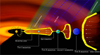 |
Fig. 1 Sketch of the global framework explored in this work. Disc evolution through angular momentum extraction by an MHD wind with additional low-level internal and external photoevaporation with accretion occurring in layers at the disc surface. Low-mass planets remain embedded and undergo type I migration. Growing planets eventually open a gap and transition to type II migration. Initially, the fast accretion layer bypasses the planet, which migrates due to Lindblad torques from the gap (viscosity-dominated regime), while still accreting. At higher masses, the planet fully blocks the flow, entering wind-driven type II migration, where it is pushed by the outer gap replenished by the accretion flow. |
2 Methods
The model is based on the Bern Model of Planet Formation and Evolution (Alibert et al. 2005; Mordasini et al. 2012; Emsenhuber et al. 2021a), including recent findings regarding planet formation in MHD wind-driven discs. The disc evolution is introduced and discussed in Sect. 2.1. Planet-disc interactions such as migration and gap-opening are described in Sect. 2.2 and the planetary growth model is introduced in Sect. 2.3.
2.1 Disc evolution model
The evolution of the gas disc was calculated using the model in Weder et al. (2023), which includes MHD wind-driven disc evolution based on Suzuki et al. (2016).
We started from an initial gas surface density profile,
![Mathematical equation: $\[\Sigma_{\mathrm{g}, \text {init}}(r)=\Sigma_{\mathrm{g}, 0,5.2 \mathrm{au}}\left(\frac{r}{5.2 ~\mathrm{au}}\right)^{-\beta} \exp \left[\left(-\frac{r}{R_{\text {char }}}\right)^{2-\beta}\right]\left(1-\sqrt{\frac{R_{\text {in}}}{r}}\right),\]$](/articles/aa/full_html/2026/02/aa57262-25/aa57262-25-eq1.png) (1)
(1)
with a power-law index of β, with Rin being the inner disc edge and characteristic radius, Rchar. Then, Σg,0,5.2au is the suitable value, where the disc mass, Mdisc, corresponds to the assigned value.
The time evolution of the integrated gas surface density, Σg, is given by the advection-diffusion equation,
![Mathematical equation: $\[\begin{aligned}\frac{\partial \Sigma_{\mathrm{g}}}{\partial t}= & \frac{1}{r} \frac{\partial}{\partial r}\left[\frac{3}{r \Omega} \frac{\partial}{\partial r}\left(r^2 \Sigma_{\mathrm{g}} \overline{\alpha_{r \phi}} c_{\mathrm{s}}^2\right)\right]+\frac{1}{r} \frac{\partial}{\partial r}\left[\frac{2}{\Omega} r \overline{\alpha_{\phi z}}\left(\rho c_{\mathrm{s}}^2\right)_{\mathrm{mid}}\right] \\& -\dot{\Sigma}_{\mathrm{MDW}}-\dot{\Sigma}_{\mathrm{PEW}, \mathrm{int}}-\dot{\Sigma}_{\mathrm{PEW}, \mathrm{ext}},\end{aligned}\]$](/articles/aa/full_html/2026/02/aa57262-25/aa57262-25-eq2.png) (2)
(2)
with r being the distance from the central star, Ω corresponding to the Keplerian frequency, and cs and ρ being sound speed and density at the disc midplane. The sink terms, ![Mathematical equation: $\[\dot{\Sigma}\]$](/articles/aa/full_html/2026/02/aa57262-25/aa57262-25-eq3.png) , correspond to various outflows; namely, the magnetic disc wind (MDW), as well as the internal and external photoevaporation (PEW). The stress acting on the disc is parameterised through
, correspond to various outflows; namely, the magnetic disc wind (MDW), as well as the internal and external photoevaporation (PEW). The stress acting on the disc is parameterised through ![Mathematical equation: $\[\overline{\alpha_{r \phi}}\]$](/articles/aa/full_html/2026/02/aa57262-25/aa57262-25-eq4.png) and
and ![Mathematical equation: $\[\overline{\alpha_{\phi z}}\]$](/articles/aa/full_html/2026/02/aa57262-25/aa57262-25-eq5.png) . The rϕ component accounts for radial transport of angular momentum through turbulence (i.e. magnetorotational instability (MRI) Balbus & Hawley 1991, 1998) and the ϕz component accounts for vertical extraction of angular momentum through the MHD wind. For simplicity, we assumed radially and temporally constant
. The rϕ component accounts for radial transport of angular momentum through turbulence (i.e. magnetorotational instability (MRI) Balbus & Hawley 1991, 1998) and the ϕz component accounts for vertical extraction of angular momentum through the MHD wind. For simplicity, we assumed radially and temporally constant ![Mathematical equation: $\[\overline{\alpha_{r \phi}}\]$](/articles/aa/full_html/2026/02/aa57262-25/aa57262-25-eq6.png) and
and ![Mathematical equation: $\[\overline{\alpha_{\phi z}}\]$](/articles/aa/full_html/2026/02/aa57262-25/aa57262-25-eq7.png) . The mass-loss rate through the magnetised wind
. The mass-loss rate through the magnetised wind ![Mathematical equation: $\[\dot{\Sigma}_{\text {MDW}}\]$](/articles/aa/full_html/2026/02/aa57262-25/aa57262-25-eq8.png) is constrained by the fraction of released gravitational energy going into launching the wind (for details on the energetic constraint, see Suzuki et al. 2016). Following the results of Weder et al. (2023) we focussed on the weak wind approach, where a fraction of the released gravitational energy is going into launching the wind (1 − ϵrad = 0.9), following Mori et al. (2025b). The remaining 10% contribute to disc heating or are radiated away.
is constrained by the fraction of released gravitational energy going into launching the wind (for details on the energetic constraint, see Suzuki et al. 2016). Following the results of Weder et al. (2023) we focussed on the weak wind approach, where a fraction of the released gravitational energy is going into launching the wind (1 − ϵrad = 0.9), following Mori et al. (2025b). The remaining 10% contribute to disc heating or are radiated away.
The assumption of a spatially and temporally constant ![Mathematical equation: $\[\overline{\alpha_{\phi z}}\]$](/articles/aa/full_html/2026/02/aa57262-25/aa57262-25-eq9.png) represents a gross simplification. The stress from the MHD wind is related to the disc magnetisation β ≡ Pth/Pmag (i.e. the ratio of thermal and magnetic pressure) and evolves with the gas density, Σg, and magnetic field strength, B (e.g. Bai & Stone 2013; Lesur 2021). However, the evolution of the magnetic field remains poorly constrained and we lack an analytical formulation. The assumption of a temporally constant
represents a gross simplification. The stress from the MHD wind is related to the disc magnetisation β ≡ Pth/Pmag (i.e. the ratio of thermal and magnetic pressure) and evolves with the gas density, Σg, and magnetic field strength, B (e.g. Bai & Stone 2013; Lesur 2021). However, the evolution of the magnetic field remains poorly constrained and we lack an analytical formulation. The assumption of a temporally constant ![Mathematical equation: $\[\overline{\alpha_{\phi z}}\]$](/articles/aa/full_html/2026/02/aa57262-25/aa57262-25-eq10.png) made here, corresponds to a constant magnetisation, β, and, hence, we have a magnetic field that dissipates at the same rate as the disc. The model used here is similar to the hybrid wind solution with Ψ > 1 and constant αDW in Tabone et al. 2022 (see their Fig. 6). The evolution of the magnetic torque has a strong impact on the evolution of the surface density in the inner disc, which can lead to a positive surface density slope that can suppress type I migration (Ogihara et al. 2015b).
made here, corresponds to a constant magnetisation, β, and, hence, we have a magnetic field that dissipates at the same rate as the disc. The model used here is similar to the hybrid wind solution with Ψ > 1 and constant αDW in Tabone et al. 2022 (see their Fig. 6). The evolution of the magnetic torque has a strong impact on the evolution of the surface density in the inner disc, which can lead to a positive surface density slope that can suppress type I migration (Ogihara et al. 2015b).
2.1.1 Accretion layer
We assume accretion to occur in an active layer at a vertical height zactive,
![Mathematical equation: $\[\Sigma_{\text {active }}=\int_{\text {zactive }}^{\infty} \rho(z) d z.\]$](/articles/aa/full_html/2026/02/aa57262-25/aa57262-25-eq11.png) (3)
(3)
The radial mass flow resulting from the wind torque is given by Eq. (34) in Suzuki et al. (2016) and expressed as
![Mathematical equation: $\[\dot{M}_{r, \phi z}(r)=-\frac{4 \pi}{\Omega} r \overline{\alpha_{\phi z}}\left(\rho c_s^2\right)_{\mathrm{mid}},\]$](/articles/aa/full_html/2026/02/aa57262-25/aa57262-25-eq12.png) (4)
(4)
with the accretion velocity ![Mathematical equation: $\[v_{\text {acc,active}}=\dot{M}_{\mathrm{r}, \phi \mathrm{z}} /\left(2 \pi r \Sigma_{\text {active}}\right)\]$](/articles/aa/full_html/2026/02/aa57262-25/aa57262-25-eq13.png) . Following Nelson et al. (2023), we can define the specific torque exerted by the wind onto the active layer,
. Following Nelson et al. (2023), we can define the specific torque exerted by the wind onto the active layer,
![Mathematical equation: $\[\Lambda_{\phi \mathrm{z}}=\frac{\mathrm{d} \Gamma_{\phi \mathrm{z}}}{\mathrm{~d} m}=\frac{1}{2} r \Omega v_{\text {acc,active }}=\frac{1}{2} r \Omega\left(\frac{\dot{M}_{\mathrm{r}, \phi \mathrm{z}}}{2 \pi r \Sigma_{\text {active }}}\right)=\frac{\Omega}{4 \pi} \frac{\dot{M}_{\mathrm{r}, \phi \mathrm{z}}}{\Sigma_{\text {active }}}.\]$](/articles/aa/full_html/2026/02/aa57262-25/aa57262-25-eq14.png) (5)
(5)
The thickness of the active layer depends on the ionisation rate (i.e. X-ray, cosmic ray and far ultraviolet (FUV) radiation) and recombination rate. We treat the layer thickness either as a constant parameter Σactive or assume accretion in the layer to occur at a fraction of sonic velocity,
![Mathematical equation: $\[\Sigma_{\text {active}}(f_{\mathrm{s}} \times c_{\mathrm{s}})=\frac{\dot{M}_{\mathrm{r}, \phi \mathrm{z}}}{2 \pi r f_{\mathrm{s}} c_{\mathrm{s}}}.\]$](/articles/aa/full_html/2026/02/aa57262-25/aa57262-25-eq15.png) (6)
(6)
The specific torque of the latter shows a much weaker scaling with orbital distance, Λϕz ∝ r−3/4 than that compared to the constant accretion layer thickness, Λϕz ∝ r−7/4.2 We point out that since the specific torque depends only on cs for Σactive (fs × cs), it will only show a very slight temporal evolution; however, for a constant Σactive, the specific torque will decrease along with the accretion rate.
2.1.2 Thermal structure
The 1D vertically integrated model makes so far no assumption to where accretion is occurring. Mori et al. (2021) developed a model for the thermal structure in a disc, where accretion and consequently accretion heating is occurring in an accretion layer. The contribution to the heating of the disc midplane is given as
![Mathematical equation: $\[T_{\mathrm{acc}, \mathrm{mid}}=\left[\left(\frac{3 F_{\mathrm{rad}}}{8 \sigma_{\mathrm{SB}}}\right)\left(\kappa_{\mathrm{R}} \Sigma_{\mathrm{heat}}+\frac{1}{\sqrt{3}}\right)\right]^{1 / 4},\]$](/articles/aa/full_html/2026/02/aa57262-25/aa57262-25-eq16.png) (7)
(7)
with κR being the Rosseland-mean opacity and Σheat being the integrated density from infinity to the bottom of the heating region, which is equivalent to Σactive (Mori et al. 2021). Gas opacities from Malygin et al. (2014) and dust opacities from Semenov et al. (2003) are used to calculate κR, following Marleau et al. (2017, 2019). The midplane temperature is given by
![Mathematical equation: $\[T_{\mathrm{mid}}=\left(T_{\mathrm{acc}, \mathrm{mid}}^4+T_{\mathrm{ext}}^4\right)^{1 / 4},\]$](/articles/aa/full_html/2026/02/aa57262-25/aa57262-25-eq17.png) (8)
(8)
with Text being the contribution due to external irradiation, such as irradiation from the star and surrounding molecular cloud (see Eqs. (3)–(5) in Weder et al. 2023).
2.1.3 Photoevaporative winds
Our model also includes outflows from internal photoevaporation by extreme ultraviolet (EUV) radiation from the host star using a diffuse stellar irradiation model (see Appendix A in Alexander & Armitage 2007). We further accounted for any shielding of the EUV radiation by the merging MHD wind (see Weder et al. 2023, for details on the shielding mechanism). We also included external photoevaporation from far ultraviolet (FUV) irradiation from surrounding stars using the FRIED grid v2 (Haworth et al. 2023). For details on the implementation, we refer to Weder et al. (2023, 2025b). Here, we adopted a low value for the ambient FUV field strength (10 G0) and polycyclic aromatic hydrocarbon (PAH) abundance of 0.1, such that the disc evolution is not strongly influenced by external photoevaporation.
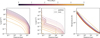 |
Fig. 2 Time evolution of an exemplary disc evolution (see Table 1 for the parameter choice). The left panel shows the evolution of the gas surface density. The evolution of the pebble and dust surface density evolution is shown in the middle panel and the right panel shows the time evolution of the midplane temperature. Note: the sudden change in dust surface density is related to the change from drift limited size (outer disc) to fragmentation limited size (inner disc). |
2.1.4 Dust evolution
For the dust evolution, we follow the two population model of dust growth from Birnstiel et al. (2012), where both dust and pebble surface density evolution are considered (Σdust(r, t) and Σpebble(r, t)). The evolution of the combined solid disc Σs = Σdust + Σpebble is calculated as a combined advection and diffusion equation. For details on the implementation we refer to Voelkel et al. (2020) and Burn et al. (2022). The surface density profiles of the two population is given at each time step as Σdust(r) = Σs(r)(1 − fm(r)) and Σpebble(r) = Σs(r)fm(r), with fm(r) being dependent on whether drift limited or fragmentation limited regime prevails. The grain sizes in the two populations are given through
![Mathematical equation: $\[a_0=10^{-5} \mathrm{cm},\]$](/articles/aa/full_html/2026/02/aa57262-25/aa57262-25-eq18.png) (9)
(9)
![Mathematical equation: $\[a_{\max }(t)=\min \left[a_{\mathrm{drift}}, a_{\mathrm{frag}}, a_0 \cdot e^{t f_{\mathrm{D} / \mathrm{G}} \Omega}\right],\]$](/articles/aa/full_html/2026/02/aa57262-25/aa57262-25-eq19.png) (10)
(10)
where the latter includes grain growth, drift and fragmentation at a threshold vfrag = 10 m/s, neglecting compositional dependencies. The fragmentation limit is correlated with the turbulent viscosity ![Mathematical equation: $\[a_{\text {frag}} \propto \Sigma_{\mathrm{g}} / \overline{\alpha_{r \phi}}\]$](/articles/aa/full_html/2026/02/aa57262-25/aa57262-25-eq20.png) , whereas the drift limited adrift ∝ Σs (Zagaria et al. 2022).
, whereas the drift limited adrift ∝ Σs (Zagaria et al. 2022).
2.1.5 Exemplary disc evolution
Figure 2 shows the time evolution of an exemplary disc. The choices for parameters are listed in Table 1. The disc has a near-infrared (NIR) lifetime of ≃4.7 Myr, which is in line with expected lifetimes of protoplanetary discs (see Weder et al. 2023, for details on the disc dispersal condition). We note the rapid increase in dust surface density that corresponds to the transition from the drift- to fragmentation-limited regime. The case presented here is similar to the hybrid case discussed in Zagaria et al. (2022). The heating of the disc midplane appears to be very ineffective and the midplane temperature is similar to a passively irradiated disc (see also Fig. 2 in Mori et al. 2025b).
Parameter choices for the exemplary case.
2.2 Planetary migration model
A schematic view of the migration regimes is given in Fig. 1. A migration map showing all the different migration regimes is shown in Fig. 3.
2.2.1 Type I migration
The migration of low-mass planets that are still embedded in the disc is not expected to be influenced by the presence of an accreting layer (McNally et al. 2020). Therefore, we used the type I migration prescription from Paardekooper et al. (2011). However, since the midplane has a low turbulent viscosity, we included the dynamical corotation torque using the memory timescale approach in (Weder et al. 2025). We note that Fig. 3 does not include the effect of the dynamical corotation torque on type I migration rates as it is partly dependent on the planet’s initial location.
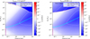 |
Fig. 3 Migration rate as a function of orbital distance and planetary mass for the exemplary disc evolution at 3 Myrs (see Sect. 2.1.5). The cyan line marks the transition from type I to type II migration through gap opening. The pink line denotes the transition into the wind-driven type II migration regime. The left panel shows the migration map for Σactive = 0.1 g/cm2 and the right panel shows the migration map for Σactive (0.08×cs). |
2.2.2 Gap opening
With increasing mass, the planet starts to perturb the gas surface density, eventually opening a deep gap. While gap formation in viscous discs has been studied extensively (Crida et al. 2006; Crida & Morbidelli 2007; Kanagawa et al. 2016, 2018), the process of gap formation in low-viscosity and MHD wind-driven discs remains unclear. Elbakyan et al. (2022) studied gap formation in discs with laminar flows driven by magnetised winds, using 2D simulations with a prescribed torque. They found that gap opening is generally determined by the residual turbulence and proposed a simple modification to the criterion from Crida et al. (2006). More recently, Aoyama & Bai (2023) and Wafflard-Fernandez & Lesur (2023) both conducted 3D global non-ideal MHD simulations including gap opening planets. Aoyama & Bai (2023) found gap shapes similar to those of inviscid discs, however, with a much great depth due to the inhomogeneous wind torque as a result to the magnetic flux concentration in the gap. This result appears to be in contrast to Wafflard-Fernandez & Lesur (2023), where it was found that higher initial magnetisation (lower β and hence higher ![Mathematical equation: $\[\overline{\overline{\alpha_{\phi \mathrm{z}}}\]$](/articles/aa/full_html/2026/02/aa57262-25/aa57262-25-eq23.png) ) leads to a higher gap opening mass (see their Fig. 5), similar to Elbakyan et al. (2022). Furthermore, the opening of deep gaps leads to steep gap edges that are Rossby-wave unstable and small scale vortices appear to diffuse the gap edges (e.g. McNally et al. 2019).
) leads to a higher gap opening mass (see their Fig. 5), similar to Elbakyan et al. (2022). Furthermore, the opening of deep gaps leads to steep gap edges that are Rossby-wave unstable and small scale vortices appear to diffuse the gap edges (e.g. McNally et al. 2019).
Given these uncertainties, we chose to use the criteria from Kanagawa et al. (2016), which does not include the dependence on the magnetic field strength. A major difference between the gap criteria from Kanagawa et al. (2016) and Crida et al. (2006) is the inclusion of the so called thermal criterion qp ≳ h3 (Lin & Papaloizou 1993). In the absence of accretion heating processes, this is in fact similar to the viscous condition for gap formation (see Fig. 4). The surface density inside the gap is given by
![Mathematical equation: $\[\frac{\Sigma_{\text {gap }}}{\Sigma_{\text {unp }}}=\frac{1}{1+0.04 K},\]$](/articles/aa/full_html/2026/02/aa57262-25/aa57262-25-eq24.png) (11)
(11)
where
![Mathematical equation: $\[K=\left(\frac{M_{\mathrm{p}}}{M_{\star}}\right)^2\left(\frac{H_{\mathrm{p}}}{r_{\mathrm{p}}}\right)^{-5} \overline{\alpha_{\mathrm{r} \phi}}-1=q^2 h_{\mathrm{p}}^{-5} \overline{\alpha_{\mathrm{r} \phi}}^{-1}.\]$](/articles/aa/full_html/2026/02/aa57262-25/aa57262-25-eq25.png) (12)
(12)
Gap opening is considered when the perturbed surface density reaches Σunp/2. Figure 4 shows the gap depth as a function of orbital distance and planetary mass for the exemplary disc discussed in Sect. 2.1.5 at 1 Myr.
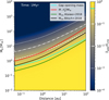 |
Fig. 4 Map showing the reduced surface density in the gap as a function of planetary mass for the exemplary disc evolution at 1 Myr (see Sect. 2.1.5), calculated using Eq. (11). The cyan line corresponds to the gap opening mass with the criterion Σgap/Σunp = 0.5. We show pebble isolation mass formulas from Bitsch et al. (2018) and Ataiee et al. (2018) in green and black and the red line corresponds to the thermal mass criterion. |
2.2.3 Type II migration
As the planet opens a gap, it eventually enters the type II migration regime. In contrast to the type I regime, the type II regime is expected to differ significantly from the classic viscous model due to the fast accretion flow and or different gap shapes. Aoyama & Bai (2023) found type II migration to be generally directed inwards and potentially affected by structures in the disc. In contrast, Wafflard-Fernandez & Lesur (2023) found sustained outward migration for Jovian planets due to asymmetric gaps and stochastic, but net slow outward migration for low-mass planets. Lega et al. (2022) found two distinct migration regimes depending on whether the planet torque onto the disc, |Λp|, exceeds the magnetic torque, |Λϕz|, which can lead to rapid inwards migration of giant planets; this is a potential explanation for the existence of hot and warm Jupiters. Here, we investigate the implication of this mechanism on a global scale, following the analytical description given in Nelson et al. (2023), where the torque density described below is used to distinguish between these two regimes.
The angular momentum exchange between planet and disc can be expressed using torque densities, Λp = dΓp/dm (D’Angelo & Lubow 2010), expressed as
![Mathematical equation: $\[\Lambda_{\mathrm{p}}=\mathcal{F}(x, \beta, \zeta) \Omega_{\mathrm{p}}^2 r_{\mathrm{p}}^2 q^2\left(\frac{r_{\mathrm{p}}}{\Delta_{\mathrm{p}}}\right)^4,\]$](/articles/aa/full_html/2026/02/aa57262-25/aa57262-25-eq26.png) (13)
(13)
with β = −d ln Σg/d ln r and ζ = −d ln T/d ln r. Δp corresponds to the maximum of the vertical scale height and the Hill radius (i.e. Δp = max(Hp, RHill)). The function ℱ is defined as
![Mathematical equation: $\[\mathcal{F}(x, \beta, \zeta)=\left[p_1 e^{-\left(x+p_2\right)^2 / p_3^2}+p_4 e^{-\left(x-p_5\right)^2 / p_6^2}\right] \cdot \tanh \left(p_7-p_8 x\right),\]$](/articles/aa/full_html/2026/02/aa57262-25/aa57262-25-eq27.png) (14)
(14)
with x = (r − rp)/Δp and pi being parameters obtained from fits (see Table 1 in D’Angelo & Lubow 2010).
Viscosity-dominated regime |Λp| < |Λϕz|. Kimmig et al. (2020) investigated the migration behaviour of giant planets in a disc with a laminar MHD wind-driven accretion flow using 2D hydrodynamical simulations. They found that replenishment of the co-orbital region can lead to a type-III-like outward migration. Their simulations suggest that this is the case if the timescale for the material to pass the librating region is sufficiently small in comparison to the libration timescale (τpass/τlib ≲ 10). However, to have outward migration, very high accretion rates through the disc have to be reached (i.e. ![Mathematical equation: $\[\dot{M}_{\mathrm{r}, \phi \mathrm{z}}\]$](/articles/aa/full_html/2026/02/aa57262-25/aa57262-25-eq28.png) ≃ 3 · 10−6 M⊙/yr), which is much higher than what we have in our simulations and we therefore neglect this process.
≃ 3 · 10−6 M⊙/yr), which is much higher than what we have in our simulations and we therefore neglect this process.
In this regime, the negative wind torque exceeds the positive planet torque and the gas flows unimpeded through the gap. We follow the approach from Kanagawa et al. (2018), where the torque onto the planet is related to Σgap. The migration rate is then given as
![Mathematical equation: $\[\dot{r}_{\mathrm{p}}=-150 \frac{\Sigma_{\mathrm{g}} r_{\mathrm{p}}}{M_{\mathrm{p}}} \overline{\alpha_{\mathrm{r} \phi}} h^3 \Omega_{\mathrm{p}}.\]$](/articles/aa/full_html/2026/02/aa57262-25/aa57262-25-eq29.png) (15)
(15)
Since ![Mathematical equation: $\[\overline{\alpha_{r \phi}}\]$](/articles/aa/full_html/2026/02/aa57262-25/aa57262-25-eq30.png) is low, gaps are deep and type II migration in this regime is slow compared to viscous discs.
is low, gaps are deep and type II migration in this regime is slow compared to viscous discs.
Wind-driven regime |Λp| > |Λϕz|. Once the planet torque exceeds the magnetic torque, the gas is halted and starts to pile up at the outer edge of the gap, leading to fast inwards migration (Lega et al. 2022). This so called wind-driven migration occurs at the rate the active layer can replenish the outer gap edge
![Mathematical equation: $\[\dot{r}_{\mathrm{p}}=\frac{\dot{M}_{\mathrm{r}, \phi \mathrm{z}}}{2 \pi r_{\mathrm{p}} \Sigma_{\mathrm{g}}}.\]$](/articles/aa/full_html/2026/02/aa57262-25/aa57262-25-eq31.png) (16)
(16)
However, we note that the planet only is expected to migrate if the the surface density of the disc is large enough. In the limit of Σg → 0, the migration rate in Eq. (16) goes to infinity. This is because we assume that the torque exerted onto a planet by the surface density of the outer gap is enough to push the planet. If we assume that the planet feels the torque exerted by the mass flow in the outer gap ![Mathematical equation: $\[\Gamma_{\mathrm{p}}=r_{\mathrm{p}}^{2} \Omega \dot{M}_{\mathrm{r}, \phi \mathrm{z}}\]$](/articles/aa/full_html/2026/02/aa57262-25/aa57262-25-eq32.png) , we get the following expression for the migration velocity,
, we get the following expression for the migration velocity,
![Mathematical equation: $\[\dot{r}_{\mathrm{p}}=\frac{2 \Gamma_{\mathrm{p}}}{M_{\mathrm{p}} r_{\mathrm{p}} \Omega}=\frac{2 r_{\mathrm{p}} \dot{M}_{\mathrm{r}, \phi \mathrm{z}}}{M_{\mathrm{p}}}\]$](/articles/aa/full_html/2026/02/aa57262-25/aa57262-25-eq33.png) (17)
(17)
The migration rate of the planet is set by the minimum of Eqs. (16) and (17), as it cannot migrate faster than the outer gap is replenished, but also does only feel the torque of the gap edge. The migration rate can thus be written as
![Mathematical equation: $\[\dot{r}_{\mathrm{p}}=\dot{M}_{\mathrm{r}, \phi \mathrm{z}} \cdot \min \left(\frac{1}{2 \pi r_{\mathrm{p}} \Sigma_{\mathrm{g}}}, \frac{2 r_{\mathrm{p}}}{M_{\mathrm{p}}}\right).\]$](/articles/aa/full_html/2026/02/aa57262-25/aa57262-25-eq34.png) (18)
(18)
We note that in the limit of a purely viscously evolving disc, the steady state accretion rate is given by ![Mathematical equation: $\[\dot{M}_{\text {acc}} \simeq 3 \pi \nu \Sigma_{\text {g}}\]$](/articles/aa/full_html/2026/02/aa57262-25/aa57262-25-eq35.png) . This naturally results in the classical migration rates for the disc- and planet dominated case (see Eq. (12) in Paardekooper et al. 2023).
. This naturally results in the classical migration rates for the disc- and planet dominated case (see Eq. (12) in Paardekooper et al. 2023).
In Fig. 3, we see the transition to the wind-driven regime at |Λp| = |Λϕz| for both a constant Σactive (left panel) and Σactive (fs × cs) (right panel). At high planetary masses the planet’s Hill radius exceeds the vertical scale height (RHill > Hp) and, thus, we can express the scaling of the planet torque as ![Mathematical equation: $\[\Lambda_{\mathrm{p}} \propto r^{-1} M_{\mathrm{p}}^{2 / 3}\]$](/articles/aa/full_html/2026/02/aa57262-25/aa57262-25-eq36.png) . Recalling the scalings of Λϕz derived in Sect. 2.1.1, this does indeed show that the critical mass scales with ∝ r0.4 for Σactive (fs × cs), whereas for a constant Σactive it is a decreasing function of orbital distance, ∝ r−1.1, and time,
. Recalling the scalings of Λϕz derived in Sect. 2.1.1, this does indeed show that the critical mass scales with ∝ r0.4 for Σactive (fs × cs), whereas for a constant Σactive it is a decreasing function of orbital distance, ∝ r−1.1, and time, ![Mathematical equation: $\[\propto \dot{M}_{\mathrm{r}, \phi \mathrm{z}}\]$](/articles/aa/full_html/2026/02/aa57262-25/aa57262-25-eq37.png) 3.
3.
2.3 Planetary accretion model
The starting point in our simulations are lunar mass embryos (10−2 M⊕) that are inserted in the disc and accrete pebbles and gas. Planetary embryos are believed to form as a result of pressure maxima (Xu & Bai 2022; Zhao et al. 2025) or streaming instability (Youdin & Goodman 2005). Spontaneous and stochastic magnetic flux concentration naturally leads to the formation of disc substructures (e.g. Riols & Lesur 2019; Riols et al. 2020), which poses a potential starting point of forming planetary embryos.
2.3.1 Pebble accretion
We simplify the solid accretion process by assuming that it occurs via pebbles (see Mordasini & Burn 2024, for a discussion of the importance of the different solid accretion mechanisms) and follow Ormel (2017) to model the accretion of pebbles. The vertical distribution of particles with Stokes number St in the gas disc is dependent on the turbulent viscosity ![Mathematical equation: $\[H_{\text {peb}}= H \sqrt{\overline{\alpha_{\mathrm{r} \phi}} /\left(\overline{\alpha_{\mathrm{r} \phi}}+\mathrm{St}\right)}\]$](/articles/aa/full_html/2026/02/aa57262-25/aa57262-25-eq38.png) . If pebbles reside in a thin layer compared to the accretion impact parameter (Hpeb ≪ bacc) the accretion rate is given as
. If pebbles reside in a thin layer compared to the accretion impact parameter (Hpeb ≪ bacc) the accretion rate is given as
![Mathematical equation: $\[\dot{M}_{2 \mathrm{D}}=2 b_{\mathrm{acc}} v_{\mathrm{enc}}\left(b_{\mathrm{acc}}\right) \Sigma_{\mathrm{peb}}.\]$](/articles/aa/full_html/2026/02/aa57262-25/aa57262-25-eq39.png) (19)
(19)
Here, bacc corresponds to the largest impact parameter that fulfils both tsettle < tenc and tstop < tenc (see Ormel 2017) and venc (bacc) is the relative encounter velocity between planet and pebble (see Eq. (7.6) in Ormel 2017). Since we here focus on discs with low turbulent viscosity, we would generally expect Hpeb ≪ bacc to be true. However, for small impact parameters (i.e. a low planetary mass) it might be the case that Hpeb ≫ bacc and the accretion rate would then be given as
![Mathematical equation: $\[\dot{M}_{\mathrm{peb}}=\dot{M}_{2 \mathrm{D}} \frac{b_{\mathrm{acc}}}{b_{\mathrm{acc}}+\sqrt{8 / \pi} H_{\mathrm{peb}}}.\]$](/articles/aa/full_html/2026/02/aa57262-25/aa57262-25-eq40.png) (20)
(20)
Pebble accretion relies on a sustained influx of pebbles from the outer disc. However, as the planet grows, it starts to influence the gas surface density and create a gap (see Sect. 2.2.2). The outer edge of the gap corresponds to a pressure bump that acts as a pebble trap. Once this so-called pebble isolation mass is reached, pebble accretion is shut off. We used the analytical prescription for the pebble isolation mass by Ataiee et al. (2018):
![Mathematical equation: $\[\left(\frac{M_{\mathrm{p}}}{M_{\star}}\right)_{\mathrm{iso}} \approx h^3 \sqrt{37.3 \overline{\alpha_{\mathrm{r} \phi}}+0.01} \times\left[1+0.2\left(\frac{\sqrt{\overline{\alpha_{\mathrm{r} \phi}}}}{h} \sqrt{\frac{1}{\mathrm{St}^2}+4}\right)^{0.7}\right].\]$](/articles/aa/full_html/2026/02/aa57262-25/aa57262-25-eq41.png) (21)
(21)
2.3.2 Gas accretion
In the attached phase, the envelope is in equilibrium with the gas disc and the accretion rate is limited by the planets ability to radiate away the liberated potential energy. Here, we calculated the gas accretion rate by solving the internal structure equations (see Sect. 4.1.1 in Emsenhuber et al. 2021a). Simultaneously, we calculated the maximum gas accretion rate following the calculations from Choksi et al. (2023) who derived scaling laws with the thermal mass, qth ≡ (Mp/M⋆)(Hp/rp)−3, expressed as
![Mathematical equation: $\[\dot{M}_{\mathrm{env}, \max }=C_i q_{\mathrm{th}, \mathrm{i}}^{a_i} h_{\mathrm{p}}^3 r_{\mathrm{p}}^3 \Omega_{\mathrm{p}} \rho_{\mathrm{gas}, \mathrm{p}},\]$](/articles/aa/full_html/2026/02/aa57262-25/aa57262-25-eq42.png) (22)
(22)
with qth, 1 ≲ 0.3 ≲ qth, 2 ≲ 10 ≲ qth, 3 with corresponding C1 = 3.5, C2 = 4/3, C3 = 9/32/3 and a1 = 2, a2 = 1, a3 = 2/3. We note that the gas density corresponds to the density at the planets location (inside the gap) ![Mathematical equation: $\[\rho_{\text {gas,} \mathrm{p}}=\Sigma_{\text {gap}} /\left(\sqrt{2 \pi} H_{\mathrm{p}}\right)\]$](/articles/aa/full_html/2026/02/aa57262-25/aa57262-25-eq43.png) . The envelope accretion rate is then given by the minimum of the two rates.
. The envelope accretion rate is then given by the minimum of the two rates.
Nelson et al. (2023) found that the accretion rate onto the planet is related to the planets ability to block the flow. In the viscosity-dominated regime (|Λp| < |Λϕz|), the planet continues to accrete at high rates, as long as the unimpeded accretion flow reaches the planet. We included this effect in an approximate way by adding the fraction of the flow that goes through the planets Hill sphere to the planet
![Mathematical equation: $\[\dot{M}_{\mathrm{env}}=\min \left(\dot{M}_{\mathrm{env}, \mathrm{attached}}, \dot{M}_{\mathrm{env}, \max }+\dot{M}_{\mathrm{r}, \phi \mathrm{z}} \frac{2 R_{\mathrm{Hill}}}{2 \pi r_{\mathrm{p}}}\right).\]$](/articles/aa/full_html/2026/02/aa57262-25/aa57262-25-eq44.png) (23)
(23)
When the planet enters the wind-driven migration regime (|Λp| > |Λϕz|), the accretion flow is blocked and accretion from the wind-driven layer (term proportional to ![Mathematical equation: $\[\dot{M}_{\mathrm{r}, \phi \mathrm{z}}\]$](/articles/aa/full_html/2026/02/aa57262-25/aa57262-25-eq45.png) ) is gradually shut down by evaluating at what distance from the planet its torque intercepts the accretion flow Rintercept and reduce the accretion rate by a factor fred = max[3/2 − Rintercept/(2RHill), 0], which is linearly decreasing out to a distance of 3 RHill, corresponding to the upper limit where the planets accrete from (Machida et al. 2010).
) is gradually shut down by evaluating at what distance from the planet its torque intercepts the accretion flow Rintercept and reduce the accretion rate by a factor fred = max[3/2 − Rintercept/(2RHill), 0], which is linearly decreasing out to a distance of 3 RHill, corresponding to the upper limit where the planets accrete from (Machida et al. 2010).
2.4 Exemplary case: Formation tracks
Figure 5 shows the formation tracks for lunar mass embryos (10−2 M⊕) inserted at t = 0 with varying initial location in the (same) exemplary disc (see Section 2.1.5 and Table 1). Each planet forms individually (no N-body interactions). Assuming that embryos are able to form anywhere in the disc at t = 0 might be a gross simplification; however, the focus of this work lies in investigating the interaction between the planets and the gas disc. Initially, the planets grow fast due to pebble accretion until they reach the pebble isolation mass and the core accretion rate goes to zero. The associated drop of the luminosity in the planet’s envelope leads to an increase of the gas accretion rate (Kessler & Alibert 2023). While the envelope is still accreting (albeit at a lower rate than the core accretion rate before) they rapidly migrate inwards (type I migration). They eventually start opening a deep gap and migration slows down (type II migration). Planets starting further out in the disc ≳10 au eventually end up in a runaway growth process. The right panels in Fig. 5 show the growth and migration rate of a planet that starts at ≃20 au. During gas runaway accretion, the migration rate starts to rapidly decrease due to the deep gap. This also eventually causes the gas accretion rate to reduce. Eventually, they enter the fast wind-driven type II migration regime. We point out that they either enter the wind-driven regime by growing or by stalling during growth, where the decreasing ![Mathematical equation: $\[\Lambda_{\phi \mathrm{z}} \propto \dot{M}_{\mathrm{r}, \phi \mathrm{z}}\]$](/articles/aa/full_html/2026/02/aa57262-25/aa57262-25-eq46.png) picks them up. This explains why planets tend to enter this regime at different masses.
picks them up. This explains why planets tend to enter this regime at different masses.
3 Single-embryo planetary population syntheses (SEPPS)
Following our discussion of the model and the resulting accretion and migration regimes at an exemplary case, we continue our assessment of the impact of different paremeterisations for Σactive on planet formation by performing single-embryo planetary population syntheses (SEPPS). We consider discs with varying initial conditions around a solar mass star, presenting the initial conditions in Sect. 3.1 and Appendix A. We give our results in Sect. 3.2.
3.1 SEPPS: Initial conditions
For the distributions of the initial conditions of the discs, we closely followed Weder et al. (2025b), as shown in Appendix A. Dust masses are inferred from a log-normal fit to Class 1 protoplanetary discs from Tychoniec et al. (2018) that is representative for stellar masses of ~0.3 M⊙. Assuming linear scaling with stellar mass, this results in log10(μ/M⊕) = 2.6 and σ = 0.35 dex. The characteristic radius is calculated using the relation Rchar = 70 au · [Mdust/100M⊕]0.25 with a 1 dex spread (Tobin et al. 2020). We used a normal distributed metallicity inferred from observations (μ = −0.02 and σ = 0.22, Santos et al. 2005) to calculate the dust-to-gas ratios using the relation fD/G = fD/G,⊙ 10[Fe/H]. The gas masses are then given by Mdust/fD/G. The strength of angular momentum transport is derived assuming a log-uniform distribution for the accretion timescale log10(τacc) = 𝒰(−0.6, 0.4). Evaluating the expression for the accretion timescale, ![Mathematical equation: $\[\tau_{\text {acc}}=M_{\text {disc}} / \dot{M}_{\text {acc}}\]$](/articles/aa/full_html/2026/02/aa57262-25/aa57262-25-eq47.png) , at the characteristic radius results in a formulation for the wind stress
, at the characteristic radius results in a formulation for the wind stress ![Mathematical equation: $\[\overline{\alpha_{\phi z}}\]$](/articles/aa/full_html/2026/02/aa57262-25/aa57262-25-eq48.png) as a function of the accretion timescale, τacc,
as a function of the accretion timescale, τacc,
![Mathematical equation: $\[\overline{\alpha_{\phi \mathrm{z}}}=\frac{M_{\mathrm{disc}}}{2 \sqrt{2 \pi} r^2 h \Omega \Sigma \tau_{\mathrm{acc}}},\]$](/articles/aa/full_html/2026/02/aa57262-25/aa57262-25-eq49.png) (24)
(24)
with h, Ω, and Σ being evaluated at the characteristic radius Rchar. For the external irradiation, we again adopted a low value of 10 G0 for the ambient FUV field strength as it was not our goal to investigate the impact of strong external photoevaporation. The actual goal is to test different values and parameterisations of the accretion layer thickness, Σactive. We adopted either a constant value for Σactive or assumed accretion to occur at a fraction of the sonic velocity, fs · cs (see Sect. 2.1.1).
Lunar mass embryos are inserted randomly in log uniform, log10(rstart) = 𝒰(log10(Rin), log(Rchar)), at the start of the simulations. This is obviously a strong simplification. However, in this paper we are primarily interested in the effects of the new disc evolution paradigm on migration and planetary growth and the formation of embryos (e.g. Voelkel et al. 2022; Lorek & Johansen 2022) is beyond the scope of this work. The key parameters are given in Table 2.
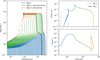 |
Fig. 5 Formation tracks compiled from 100 individual single embryo simulations (Memb = 10−2 M⊕) with varying initial locations rstart spaced uniform in log between 0.05 au and 40 au for our exemplary disc discussed in Section 2.1.5. The tracks are coloured by migration regime. Time evolution of the planet’s accretion rate (core and envelope) and migration rate are shown as an example for a planet with rstart ≃ 20 au. |
3.2 SEPPS: Results
We ran populations of 1000 simulations each with varying initial disc conditions and embryo starting locations distributed randomly in log for different parameterisations of Σactive. Simulations were run until the dispersion of the disc. We would like to point out that the initial conditions of the disc result in disc lifetimes that are in agreement with observations (see panel f in Fig. A.1).
Figure 6 shows the resulting distance-mass diagram of the different populations along 100 simulation tracks coloured by migration regimes for visualisation. At a very basic level, the distance-mass diagrams do not look fundamentally different from observations; namely, there are many close-in low-mass planets, distant giants, and potentially some close-in giants, depending on the accretion layer thickness Σactive.
Based on Fig. 6, we made the following observations.
- (i)
For thin accretion layers (i.e. Σactive = 10−2 g/cm2 and fs = 0.12), planetary growth halts before they reach the wind-driven type 2 migration regime. This shows that the planetary mass function at the high end is set by deep gap opening, which makes it difficult to grow past ~103 M⊕. This corresponds to the case where the wind-driven regime (Eq. (16)) is ignored and migration is solely due to the viscosity-dominated regime (Eq. (17));
- (ii)
For an intermediate layer thickness (i.e. Σactive = 10−1 g/cm2 and fs = 0.08), the influence on the giant planet populations starts to emerge with some giant planets migrating far in, before the disc eventually disperses. We note that for Σactive(0.08 × cs), Λϕz is remaining at a constant value, and planets eventually enter wind-driven migration at high masses. For the case with Σactive = 0.1 g/cm2, the critical mass where |Λp| > |Λϕz| decreases with
![Mathematical equation: $\[\propto \dot{M}_{\mathrm{r}, \phi \mathrm{z}}\]$](/articles/aa/full_html/2026/02/aa57262-25/aa57262-25-eq52.png) and, hence, even planets at masses ~102 M⊕ are influenced;
and, hence, even planets at masses ~102 M⊕ are influenced; - (iii)
For thick accretion layers (i.e. Σactive = 1 g/cm2), the influence is clearly visible. Some of the giant planets intercept the accretion layer during their growth, stop accreting and start migrating inwards rapidly, which can be seen in the planetary mass distribution Fig. 7. This leads to many close in giant planets and few to none giant planets outside of 1 au;
- (iv)
For Σactive (0.03 × cs), the critical mass is again lower as for panel e) and planets enter the wind-driven migration regime during the runaway growth phase, leading to an upper limit of the mass distribution at about 330 M⊕ in Fig. 7.
Some of the planets with masses 20 M⊕ ≲ Mp ≲ 200 M⊕ show a sudden drop in mass due to the loss of their envelope. Young hot giant planets migrated far in are suddenly exposed to direct stellar irradiation, Firr, leading to bloating, driving atmospheric escape, ![Mathematical equation: $\[\dot{M} \propto F_{\text {irr}} / \rho\]$](/articles/aa/full_html/2026/02/aa57262-25/aa57262-25-eq53.png) , in a runaway fashion (Baraffe et al. 2004; Sarkis et al. 2021; Thorngren et al. 2023). This process then leads to the near-vertical drop in planetary mass observed in some cases.
, in a runaway fashion (Baraffe et al. 2004; Sarkis et al. 2021; Thorngren et al. 2023). This process then leads to the near-vertical drop in planetary mass observed in some cases.
With the population syntheses, it is possible to see how physical processes and model parameters such as the layer thickness imprint into the demographics of the exoplanet population, which can in part be observed. By running a single embryo population, we can identify these imprints more clearly. For a detailed comparison with observations, a multi-embryo approach would be needed (Burn & Mordasini 2024). It is, however, still interesting to qualitatively compare some imprints found here with observations.
Planetary population synthesis models have predicted a planetary desert (Ida & Lin 2004) at intermediate masses of 20–200 M⊕ that is caused by the high gas accretion rate in the runaway phase. Clear observational evidence of the existence of such a planetary desert is being discussed with some studies pointing towards such a feature (Mayor et al. 2011; Bertaux & Ivanova 2022; Zang et al. 2025) and others discarding it (Suzuki et al. 2018; Bennett et al. 2021). Our simulations show that such a feature persists (see Fig. 7), where a minimum in the planetary mass function appears around ~10–20 M⊕ which is lower than the observed ~40 M⊕ (Figure 5 in Emsenhuber et al. 2025) and lower than what was found in previous planetary population syntheses using viscous disc evolution (e.g. Emsenhuber et al. 2025, NGPPS). In our simulation, the desert is a result of gas runaway accretion, but the location ~10–20 M⊕ is set by the low pebble isolation and absence of delay of runaway accretion due to higher core masses by planetesimal accretion.
The maximum of the distribution of giant planet masses is at ~300 M⊕, which is in good agreement with observations, whereas past NGPPS simulations with viscous discs overestimated the giant planet masses Emsenhuber et al. (2025). On the other hand, we obtain a sharp drop of the mass function at ~103 M⊕ as already mentioned above, which stands in contrast to the observations. In the NGPPS simulations with viscous discs, this upper end was in contrast well reproduced. We can speculate whether additional mechanisms that are not included here could also be enabling giant planet growth to higher masses in low-viscosity discs. One possibility could be the eccentric instability Papaloizou et al. (2001); Kley & Dirksen (2006), which could be more easily excited in low-viscosity discs with deep and wide gaps.
Figure 7 also shows that although the distance-mass diagrams of panels a) and b) appear vastly different, the mass distributions are similar, suggesting that the planets have already stopped growing when they entered the wind-driven type II migration regime; this is possible due to the ![Mathematical equation: $\[\Lambda_{\phi \mathrm{z}} \propto \dot{M}_{\mathrm{r}, \phi \mathrm{z}}\]$](/articles/aa/full_html/2026/02/aa57262-25/aa57262-25-eq54.png) dependence of the wind torque. In the case of Σactive (fs × cs), we see that the upper limit of the planetary masses in the population is decreasing with lower fs, meaning that the planets are entering the wind-driven migration regime during their growth phase.
dependence of the wind torque. In the case of Σactive (fs × cs), we see that the upper limit of the planetary masses in the population is decreasing with lower fs, meaning that the planets are entering the wind-driven migration regime during their growth phase.
Theoretical constraints on accretion layer thickness remain sparse. Mori et al. (2021) reported values of Σactive ≈ 0.1–0.6 g/cm2, while simulations from Mori et al. (2025a) show slightly subsonic accretion in the active layer. These values are well within the range of where wind-driven type II migration could play a role for the orbital distance of giant planets, making it an additional mechanism to high eccentricity migration (Wu & Murray 2003), which could explain close in giant planets.
Interestingly enough, our simulation allow us to set independent, observationally motivated constraints on the layer thickness via the comparison with the observed demographics of extrasolar giant planets. It is clear that this constraint must be taken with care due to the various limitations of the model. Still, when taking the six distance-mass diagrams shown in Fig. 6 at face value, it is evident that the simulations with the thinnest layer thicknesses (left panels of Fig. 6) are not in agreement with the observations as they do not produce any hot Jupiters. Some of the observed hot Jupiters that are found close-in very early on are coplanar with the star and have smaller bodies in mean motion resonance which is a clear indication of disc migration leading to their current position (Hord et al. 2022). Similarly, the thickest layers (right panels of Fig. 6) are in disagreement with observations as they lead to far too many hot Jupiters compared to the cold Jupiters (i.e. the observed frequency of the former is about 0.5%, of the latter about 20%, as reported in the literature (Fulton et al. 2021)).
The intermediate cases (middle panels of Fig. 6) finally demonstrate that for a distribution active layers with thicknesses that are of the order of 0.1 g/cm2 (agreeing with Mori et al. 2021) or with velocities of the order of 10% of the sound speed or a plausible diversity among the accretion layer thicknesses, it is possible to obtain a ratio of hot-to-cold Jupiters that would be in agreement with observations.
Summary of the parameter choice and initial distributions of the variables for the SEPPS.
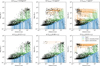 |
Fig. 6 Distance–mass diagrams for single-embryo populations with varying parameterisations of Σactive. Top row shows results for temporally and spatially constant Σactive, while the bottom row shows results with the accretion velocity being a fraction of the local sound speed, fs × cs. Accretion layer thicknesses increase from left to right. Formation tracks are shown for 200 randomly selected simulations coloured by migration regime. |
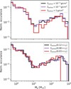 |
Fig. 7 Normalised distribution of planetary masses for the populations shown in Fig. 6. While the overall shape is similar, there are less massive giant planets for slow accretion velocities (≲0.08 × cs). |
4 Summary and conclusions
We have assembled several key aspects of MHD wind-driven discs, including the effects of laminar surface layer accretion on planetary migration and accretion, proposed by Lega et al. (2022) and Nelson et al. (2023) into a global planet formation model. We performed single-embryo planetary population syntheses within this new disc evolution paradigm and we investigated the impact of different parameterisations for the thickness of the accreting layer, Σactive. We present the following conclusions based on our model:
On a very basic level, the paradigm of layered MHD wind-driven discs with planet formation via core accretion including pebble accretion leads to populations that share the key properties of the observed planet population (numerous close-in low-mass and outer, less numerous giant planets, whose locations depend on the specific layer thickness);
The thickness of the active layer has a large impact on the final location of giant planets. The thicker the layer, the more giant planets migrate close to their host star. Fast, wind-driven type II migration could pose an alternative origin to close in giant planets in addition to high eccentricity migration;
A detailed quantitative comparison with the exoplanet population is beyond the scope of this work and would require to include more physical processes. However, if we take the results obtained here at face value, then we would find that the resulting synthetic distance-mass diagrams are in agreement with the observed one in terms of the relative frequency of hot-versus-cold Jupiters for a layer thickness on the order of 0.1 g/cm2 or velocity of approximately 10% of cs. Clearly, thinner or faster layers are incompatible because no hot Jupiters would form at all and thicker or slower layers would lead to the opposite case, namely, too many close-in giants;
Time and location of the critical mass for entering wind-driven type II migration poses a hard limit to upper end of the final mass distribution of giant planets, favouring also rather fast ≳ 0.1 × cs and thin accretion layers ≤ 0.1 g/cm2;
In the absence of wind-driven type II migration (i.e. for very thin accretion layers), we find type II migration to be inefficient due to deep gap opening, leading to a bifurcation of low mass planets forming further in and high-mass planets forming further out in the disc. This specifically means that in low-viscosity discs without an active layer at all (or a very thin one), hot Jupiter formation via disc migration is not possible. Giant planets grow, once they have started runaway gas accretion, virtually in situ;
Using current gap opening criteria and gas accretion rates derived from hydrodynamic simulations, it is difficult to grow past ≳103 M⊕ in low viscosity (
![Mathematical equation: $\[\overline{\alpha_{r \phi}}\]$](/articles/aa/full_html/2026/02/aa57262-25/aa57262-25-eq55.png) = 10−4) due to efficient and deep gap opening. This is in contrast to the observed upper end of the planetary mass function. Alternative physical mechanisms not included here, such as the eccentric instability (Papaloizou et al. 2001; Kley & Dirksen 2006), could allow for growth to higher masses.
= 10−4) due to efficient and deep gap opening. This is in contrast to the observed upper end of the planetary mass function. Alternative physical mechanisms not included here, such as the eccentric instability (Papaloizou et al. 2001; Kley & Dirksen 2006), could allow for growth to higher masses.
Many questions remain regarding planet formation in MHD wind-driven discs that have to be addressed using 2D and 3D magnetohydrodynamic simulations. These results should then be broken down to 1D for inclusion in global models to allow for statistical comparisons with observations. A key question is the formation and depth of gaps and how planets located in these gaps accrete gas. Furthermore, type II migration is closely related to the gap formation process and remains highly uncertain with results differing between models (Lega et al. 2022; Aoyama & Bai 2023; Wafflard-Fernandez & Lesur 2023). Finding analytic expressions for the migration rates (e.g. outward migration found by Wafflard-Fernandez & Lesur 2023) would allow us to test the implications of such migration behaviour on planet formation in a global view, similarly as we have done in this work.
Our simulations already show some distinctions from synthetic populations in viscous discs and draw a picture that is similar to what was proposed in Ziampras et al. (2025). In this work, we neglected any effects from the radial dependence and time evolution of the wind torque, ![Mathematical equation: $\[\overline{\alpha_{\phi \mathrm{z}}}\]$](/articles/aa/full_html/2026/02/aa57262-25/aa57262-25-eq56.png) , and turbulent viscosity,
, and turbulent viscosity, ![Mathematical equation: $\[\overline{\alpha_{r \phi}}\]$](/articles/aa/full_html/2026/02/aa57262-25/aa57262-25-eq57.png) , that can lead to inner cavities and migration traps (e.g. Ogihara et al. 2015b; Flock et al. 2019; Speedie et al. 2022; Alessi & Pudritz 2022). These effects strongly depend on the thermal physics of the disc and the magnetic field configuration, where the latter remains poorly constrained. Testing existing constraints (e.g. Lesur 2021; Kobayashi et al. 2025) using planetary population syntheses approach will offer valuable insights that will help in assessing our current store of knowledge. These areas will be the subject of future studies.
, that can lead to inner cavities and migration traps (e.g. Ogihara et al. 2015b; Flock et al. 2019; Speedie et al. 2022; Alessi & Pudritz 2022). These effects strongly depend on the thermal physics of the disc and the magnetic field configuration, where the latter remains poorly constrained. Testing existing constraints (e.g. Lesur 2021; Kobayashi et al. 2025) using planetary population syntheses approach will offer valuable insights that will help in assessing our current store of knowledge. These areas will be the subject of future studies.
Acknowledgements
We would like to thank Elena Lega, Aurélien Crida, Alessandro Morbidelli and Richard Nelson for fruitful discussions. We would also like to thank Shoji Mori for providing more insights on the results on accretion layer from 2D magnetohydrodynamic simulations. We would like to thank the referee for their useful comments that greatly helped improving the clarity of the manuscript. We further thank Alessandro Morbidelli for a thorough reading of a first version of this manuscript. J.W. and C.M. acknowledge the support from the Swiss National Science Foundation under grant 200021_204847 “PlanetsInTime”. Part of this work has been carried out within the framework of the NCCR PlanetS supported by the Swiss National Science Foundation under grants 51NF40_182901 and 51NF40_205606. Calculations were performed on the Horus cluster of the Division of Space Research and Planetary Sciences at the University of Bern.
References
- Alessi, M., & Pudritz, R. E. 2018, MNRAS, 478, 2599 [NASA ADS] [CrossRef] [Google Scholar]
- Alessi, M., & Pudritz, R. E. 2022, MNRAS, 515, 2548 [NASA ADS] [CrossRef] [Google Scholar]
- Alexander, R. D., & Armitage, P. J. 2007, MNRAS, 375, 500 [NASA ADS] [CrossRef] [Google Scholar]
- Alibert, Y., Mordasini, C., & Benz, W. 2004, A&A, 417, L25 [NASA ADS] [CrossRef] [EDP Sciences] [Google Scholar]
- Alibert, Y., Mordasini, C., Benz, W., & Winisdoerffer, C. 2005, A&A, 434, 343 [NASA ADS] [CrossRef] [EDP Sciences] [Google Scholar]
- Alibert, Y., Carron, F., Fortier, A., et al. 2013, A&A, 558, A109 [NASA ADS] [CrossRef] [EDP Sciences] [Google Scholar]
- Aoyama, Y., & Bai, X.-N. 2023, ApJ, 946, 5 [NASA ADS] [CrossRef] [Google Scholar]
- Ataiee, S., Baruteau, C., Alibert, Y., & Benz, W. 2018, A&A, 615, A110 [NASA ADS] [CrossRef] [EDP Sciences] [Google Scholar]
- Bai, X.-N., & Stone, J. M. 2013, ApJ, 769, 76 [Google Scholar]
- Balbus, S. A., & Hawley, J. F. 1991, ApJ, 376, 214 [Google Scholar]
- Balbus, S. A., & Hawley, J. F. 1998, Rev. Mod. Phys., 70, 1 [Google Scholar]
- Baraffe, I., Selsis, F., Chabrier, G., et al. 2004, A&A, 419, L13 [NASA ADS] [CrossRef] [EDP Sciences] [Google Scholar]
- Bennett, D. P., Ranc, C., & Fernandes, R. B. 2021, AJ, 162, 243 [NASA ADS] [CrossRef] [Google Scholar]
- Bertaux, J.-L., & Ivanova, A. 2022, MNRAS, 512, 5552 [NASA ADS] [CrossRef] [Google Scholar]
- Birnstiel, T., Klahr, H., & Ercolano, B. 2012, A&A, 539, A148 [NASA ADS] [CrossRef] [EDP Sciences] [Google Scholar]
- Bitsch, B., Lambrechts, M., & Johansen, A. 2015, A&A, 582, A112 [NASA ADS] [CrossRef] [EDP Sciences] [Google Scholar]
- Bitsch, B., Morbidelli, A., Johansen, A., et al. 2018, A&A, 612, A30 [NASA ADS] [CrossRef] [EDP Sciences] [Google Scholar]
- Blandford, R. D., & Payne, D. G. 1982, MNRAS, 199, 883 [CrossRef] [Google Scholar]
- Brügger, N., Alibert, Y., Ataiee, S., & Benz, W. 2018, A&A, 619, A174 [Google Scholar]
- Burn, R., & Mordasini, C. 2024, in Handbook of Exoplanets, 143–2 [Google Scholar]
- Burn, R., Emsenhuber, A., Weder, J., et al. 2022, A&A, 666, A73 [NASA ADS] [CrossRef] [EDP Sciences] [Google Scholar]
- Choksi, N., Chiang, E., Fung, J., & Zhu, Z. 2023, MNRAS, 525, 2806 [Google Scholar]
- Crida, A., & Morbidelli, A. 2007, MNRAS, 377, 1324 [Google Scholar]
- Crida, A., Morbidelli, A., & Masset, F. 2006, Icarus, 181, 587 [Google Scholar]
- D’Angelo, G., & Lubow, S. H. 2010, ApJ, 724, 730 [Google Scholar]
- Drążkowska, J., Bitsch, B., Lambrechts, M., et al. 2023, in Astronomical Society of the Pacific Conference Series, 534, Protostars and Planets VII, eds. S. Inutsuka, Y. Aikawa, T. Muto, K. Tomida, & M. Tamura, 717 [Google Scholar]
- Elbakyan, V., Wu, Y., Nayakshin, S., & Rosotti, G. 2022, MNRAS, 515, 3113 [NASA ADS] [CrossRef] [Google Scholar]
- Emsenhuber, A., Mordasini, C., Burn, R., et al. 2021a, A&A, 656, A69 [NASA ADS] [CrossRef] [EDP Sciences] [Google Scholar]
- Emsenhuber, A., Mordasini, C., Burn, R., et al. 2021b, A&A, 656, A70 [NASA ADS] [CrossRef] [EDP Sciences] [Google Scholar]
- Emsenhuber, A., Mordasini, C., Mayor, M., et al. 2025, A&A, 701, A64 [NASA ADS] [CrossRef] [EDP Sciences] [Google Scholar]
- Flock, M., Turner, N. J., Mulders, G. D., et al. 2019, A&A, 630, A147 [NASA ADS] [CrossRef] [EDP Sciences] [Google Scholar]
- Fulton, B. J., Rosenthal, L. J., Hirsch, L. A., et al. 2021, ApJS, 255, 14 [NASA ADS] [CrossRef] [Google Scholar]
- Haworth, T. J., Coleman, G. A. L., Qiao, L., Sellek, A. D., & Askari, K. 2023, MNRAS, 526, 4315 [NASA ADS] [CrossRef] [Google Scholar]
- Hord, B. J., Colón, K. D., Berger, T. A., et al. 2022, AJ, 164, 13 [NASA ADS] [CrossRef] [Google Scholar]
- Hu, X., Li, Z.-Y., Bae, J., & Zhu, Z. 2025, MNRAS, 536, 1374 [NASA ADS] [Google Scholar]
- Ida, S., & Lin, D. N. C. 2004, ApJ, 604, 388 [Google Scholar]
- Kanagawa, K. D., Muto, T., Tanaka, H., et al. 2016, PASJ, 68, 43 [NASA ADS] [Google Scholar]
- Kanagawa, K. D., Tanaka, H., & Szuszkiewicz, E. 2018, ApJ, 861, 140 [Google Scholar]
- Kessler, A., & Alibert, Y. 2023, A&A, 674, A144 [NASA ADS] [CrossRef] [EDP Sciences] [Google Scholar]
- Kimmig, C. N., Dullemond, C. P., & Kley, W. 2020, A&A, 633, A4 [NASA ADS] [CrossRef] [EDP Sciences] [Google Scholar]
- Kimura, T., & Ikoma, M. 2022, Nat. Astron., 6, 1296 [NASA ADS] [CrossRef] [Google Scholar]
- Kimura, S. S., Kunitomo, M., & Takahashi, S. Z. 2016, MNRAS, 461, 2257 [NASA ADS] [CrossRef] [Google Scholar]
- Kley, W., & Dirksen, G. 2006, A&A, 447, 369 [NASA ADS] [CrossRef] [EDP Sciences] [Google Scholar]
- Kobayashi, Y., Takaishi, D., Tsukamoto, Y., & Basu, S. 2025, ApJ, 990, 95 [Google Scholar]
- Lega, E., Morbidelli, A., Nelson, R. P., et al. 2022, A&A, 658, A32 [NASA ADS] [CrossRef] [EDP Sciences] [Google Scholar]
- Lesur, G. R. J. 2021, A&A, 650, A35 [NASA ADS] [CrossRef] [EDP Sciences] [Google Scholar]
- Lin, D. N. C., & Papaloizou, J. C. B. 1993, in Protostars and Planets III, eds. E. H. Levy, & J. I. Lunine, 749 [Google Scholar]
- Lorek, S., & Johansen, A. 2022, A&A, 666, A108 [NASA ADS] [CrossRef] [EDP Sciences] [Google Scholar]
- Machida, M. N., Kokubo, E., Inutsuka, S.-I., & Matsumoto, T. 2010, MNRAS, 405, 1227 [Google Scholar]
- Malygin, M. G., Kuiper, R., Klahr, H., Dullemond, C. P., & Henning, T. 2014, A&A, 568, A91 [NASA ADS] [CrossRef] [EDP Sciences] [Google Scholar]
- Manara, C. F., Ansdell, M., Rosotti, G. P., et al. 2023, in Astronomical Society of the Pacific Conference Series, Vol. 534, Protostars and Planets VII, eds. S. Inutsuka, Y. Aikawa, T. Muto, K. Tomida, & M. Tamura, 539 [Google Scholar]
- Marleau, G.-D., Klahr, H., Kuiper, R., & Mordasini, C. 2017, ApJ, 836, 221 [Google Scholar]
- Marleau, G.-D., Mordasini, C., & Kuiper, R. 2019, ApJ, 881, 144 [Google Scholar]
- Mayor, M., Marmier, M., Lovis, C., et al. 2011, arXiv e-prints [arXiv:1109.2497] [Google Scholar]
- McNally, C. P., Nelson, R. P., Paardekooper, S.-J., & Benítez-Llambay, P. 2019, MNRAS, 484, 728 [Google Scholar]
- McNally, C. P., Nelson, R. P., Paardekooper, S.-J., Benítez-Llambay, P., & Gressel, O. 2020, MNRAS, 493, 4382 [NASA ADS] [CrossRef] [Google Scholar]
- Miotello, A., Kamp, I., Birnstiel, T., Cleeves, L. C., & Kataoka, A. 2023, in Astronomical Society of the Pacific Conference Series, 534, Protostars and Planets VII, eds. S. Inutsuka, Y. Aikawa, T. Muto, K. Tomida, & M. Tamura, 501 [Google Scholar]
- Mordasini, C., & Burn, R. 2024, Rev. Mineral. Geochem., 90, 55 [Google Scholar]
- Mordasini, C., Alibert, Y., & Benz, W. 2009a, A&A, 501, 1139 [CrossRef] [EDP Sciences] [Google Scholar]
- Mordasini, C., Alibert, Y., Benz, W., & Naef, D. 2009b, A&A, 501, 1161 [NASA ADS] [CrossRef] [EDP Sciences] [Google Scholar]
- Mordasini, C., Alibert, Y., Klahr, H., & Henning, T. 2012, A&A, 547, A111 [NASA ADS] [CrossRef] [EDP Sciences] [Google Scholar]
- Mori, S., Bai, X.-N., & Okuzumi, S. 2019, ApJ, 872, 98 [NASA ADS] [CrossRef] [Google Scholar]
- Mori, S., Bai, X.-N., & Tomida, K. 2025a, ApJ, 992, 85 [Google Scholar]
- Mori, S., Okuzumi, S., Kunitomo, M., & Bai, X.-N. 2021, ApJ, 916, 72 [NASA ADS] [CrossRef] [Google Scholar]
- Mori, S., Kunitomo, M., & Ogihara, M. 2025b, A&A, 697, A192 [NASA ADS] [CrossRef] [EDP Sciences] [Google Scholar]
- Nelson, R. P., Lega, E., & Morbidelli, A. 2023, A&A, 670, A113 [NASA ADS] [CrossRef] [EDP Sciences] [Google Scholar]
- Ogihara, M., Kobayashi, H., Inutsuka, S.-i., & Suzuki, T. K. 2015a, A&A, 579, A65 [NASA ADS] [CrossRef] [EDP Sciences] [Google Scholar]
- Ogihara, M., Morbidelli, A., & Guillot, T. 2015b, A&A, 584, L1 [NASA ADS] [CrossRef] [EDP Sciences] [Google Scholar]
- Ormel, C. W. 2017, in Astrophysics and Space Science Library, 445, Formation, Evolution, and Dynamics of Young Solar Systems, eds. M. Pessah, & O. Gressel, 197 [Google Scholar]
- Paardekooper, S. J., Baruteau, C., & Kley, W. 2011, MNRAS, 410, 293 [NASA ADS] [CrossRef] [Google Scholar]
- Papaloizou, J. C. B., Nelson, R. P., & Masset, F. 2001, A&A, 366, 263 [NASA ADS] [CrossRef] [EDP Sciences] [Google Scholar]
- Paardekooper, S., Dong, R., Duffell, P., et al. 2023, in Astronomical Society of the Pacific Conference Series, 534, Protostars and Planets VII, eds. S. Inutsuka, Y. Aikawa, T. Muto, K. Tomida, & M. Tamura, 685 [Google Scholar]
- Riols, A., & Lesur, G. 2019, A&A, 625, A108 [NASA ADS] [CrossRef] [EDP Sciences] [Google Scholar]
- Riols, A., Lesur, G., & Menard, F. 2020, A&A, 639, A95 [NASA ADS] [CrossRef] [EDP Sciences] [Google Scholar]
- Santos, N. C., Israelian, G., Mayor, M., et al. 2005, A&A, 437, 1127 [NASA ADS] [CrossRef] [EDP Sciences] [Google Scholar]
- Sarkis, P., Mordasini, C., Henning, T., Marleau, G. D., & Mollière, P. 2021, A&A, 645, A79 [NASA ADS] [CrossRef] [EDP Sciences] [Google Scholar]
- Semenov, D., Henning, T., Helling, C., Ilgner, M., & Sedlmayr, E. 2003, A&A, 410, 611 [NASA ADS] [CrossRef] [EDP Sciences] [Google Scholar]
- Speedie, J., Pudritz, R. E., Cridland, A. J., Meru, F., & Booth, R. A. 2022, MNRAS, 510, 6059 [Google Scholar]
- Suzuki, T. K., Ogihara, M., Morbidelli, A., Crida, A., & Guillot, T. 2016, A&A, 596, A74 [NASA ADS] [CrossRef] [EDP Sciences] [Google Scholar]
- Suzuki, D., Bennett, D. P., Ida, S., et al. 2018, ApJ, 869, L34 [NASA ADS] [CrossRef] [Google Scholar]
- Tabone, B., Rosotti, G. P., Cridland, A. J., Armitage, P. J., & Lodato, G. 2022, MNRAS, 512, 2290 [NASA ADS] [CrossRef] [Google Scholar]
- Thorngren, D. P., Lee, E. J., & Lopez, E. D. 2023, ApJ, 945, L36 [NASA ADS] [CrossRef] [Google Scholar]
- Tobin, J. J., Sheehan, P. D., Megeath, S. T., et al. 2020, ApJ, 890, 130 [CrossRef] [Google Scholar]
- Tychoniec, Ł., Tobin, J. J., Karska, A., et al. 2018, ApJS, 238, 19 [Google Scholar]
- Voelkel, O., Klahr, H., Mordasini, C., & Emsenhuber, A. 2022, A&A, 666, A90 [NASA ADS] [CrossRef] [EDP Sciences] [Google Scholar]
- Voelkel, O., Klahr, H., Mordasini, C., Emsenhuber, A., & Lenz, C. 2020, A&A, 642, A75 [NASA ADS] [CrossRef] [EDP Sciences] [Google Scholar]
- Wafflard-Fernandez, G., & Lesur, G. 2023, A&A, 677, A70 [NASA ADS] [CrossRef] [EDP Sciences] [Google Scholar]
- Wafflard-Fernandez, G., & Lesur, G. 2025, A&A, 696, A8 [NASA ADS] [CrossRef] [EDP Sciences] [Google Scholar]
- Weder, J., Mordasini, C., & Emsenhuber, A. 2023, A&A, 674, A165 [NASA ADS] [CrossRef] [EDP Sciences] [Google Scholar]
- Weder, J., Baruteau, C., & Mordasini, C. 2025, A&A, 701, A16 [NASA ADS] [CrossRef] [EDP Sciences] [Google Scholar]
- Weder, J., Winter, A. J., & Mordasini, C. 2026, A&A, 705, A102 [NASA ADS] [CrossRef] [EDP Sciences] [Google Scholar]
- Wu, Y., & Chen, Y.-X. 2025, MNRAS, 536, L13 [Google Scholar]
- Wu, Y., & Murray, N. 2003, ApJ, 589, 605 [Google Scholar]
- Xu, Z., & Bai, X.-N. 2022, ApJ, 937, L4 [NASA ADS] [CrossRef] [Google Scholar]
- Youdin, A. N., & Goodman, J. 2005, ApJ, 620, 459 [Google Scholar]
- Zagaria, F., Rosotti, G. P., Clarke, C. J., & Tabone, B. 2022, MNRAS, 514, 1088 [CrossRef] [Google Scholar]
- Zang, W., Jung, Y. K., Yee, J. C., et al. 2025, Science, 388, 400 [Google Scholar]
- Zhao, H., Lau, T. C. H., Birnstiel, T., Stammler, S. M., & Drążkowska, J. 2025, A&A, 694, A205 [NASA ADS] [CrossRef] [EDP Sciences] [Google Scholar]
- Ziampras, A., Nelson, R. P., & Paardekooper, S.-J. 2025, MNRAS, 542, 1685 [Google Scholar]
As of August 2025, according to https://exoplanet.eu
For these scalings we assumed Σg ∝ r−1 and a temperature profile of a passively irradiated disc Tmid ∝ r−1/2.
Note that the scaling with r is less precise for constant Σactive as the dependencies on ![Mathematical equation: $\[\dot{M}_{\phi \mathrm{z}}\]$](/articles/aa/full_html/2026/02/aa57262-25/aa57262-25-eq58.png) and Σg do not cancel out when comparing Λp and Λϕz and hence the assumptions made in Sect. 2.1.1 may not hold after some time.
and Σg do not cancel out when comparing Λp and Λϕz and hence the assumptions made in Sect. 2.1.1 may not hold after some time.
Appendix A Distributions of the initial conditions for the population and resulting disc lifetime distribution
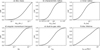 |
Fig. A.1 Distributions of the initial disc conditions according to Sect. 3.1. Resulting NIR disc lifetimes according to Kimura et al. (2016) are shown in panel f). |
All Tables
Summary of the parameter choice and initial distributions of the variables for the SEPPS.
All Figures
|
Fig. 1 Sketch of the global framework explored in this work. Disc evolution through angular momentum extraction by an MHD wind with additional low-level internal and external photoevaporation with accretion occurring in layers at the disc surface. Low-mass planets remain embedded and undergo type I migration. Growing planets eventually open a gap and transition to type II migration. Initially, the fast accretion layer bypasses the planet, which migrates due to Lindblad torques from the gap (viscosity-dominated regime), while still accreting. At higher masses, the planet fully blocks the flow, entering wind-driven type II migration, where it is pushed by the outer gap replenished by the accretion flow. |
| In the text | |
|
Fig. 2 Time evolution of an exemplary disc evolution (see Table 1 for the parameter choice). The left panel shows the evolution of the gas surface density. The evolution of the pebble and dust surface density evolution is shown in the middle panel and the right panel shows the time evolution of the midplane temperature. Note: the sudden change in dust surface density is related to the change from drift limited size (outer disc) to fragmentation limited size (inner disc). |
| In the text | |
|
Fig. 3 Migration rate as a function of orbital distance and planetary mass for the exemplary disc evolution at 3 Myrs (see Sect. 2.1.5). The cyan line marks the transition from type I to type II migration through gap opening. The pink line denotes the transition into the wind-driven type II migration regime. The left panel shows the migration map for Σactive = 0.1 g/cm2 and the right panel shows the migration map for Σactive (0.08×cs). |
| In the text | |
|
Fig. 4 Map showing the reduced surface density in the gap as a function of planetary mass for the exemplary disc evolution at 1 Myr (see Sect. 2.1.5), calculated using Eq. (11). The cyan line corresponds to the gap opening mass with the criterion Σgap/Σunp = 0.5. We show pebble isolation mass formulas from Bitsch et al. (2018) and Ataiee et al. (2018) in green and black and the red line corresponds to the thermal mass criterion. |
| In the text | |
|
Fig. 5 Formation tracks compiled from 100 individual single embryo simulations (Memb = 10−2 M⊕) with varying initial locations rstart spaced uniform in log between 0.05 au and 40 au for our exemplary disc discussed in Section 2.1.5. The tracks are coloured by migration regime. Time evolution of the planet’s accretion rate (core and envelope) and migration rate are shown as an example for a planet with rstart ≃ 20 au. |
| In the text | |
|
Fig. 6 Distance–mass diagrams for single-embryo populations with varying parameterisations of Σactive. Top row shows results for temporally and spatially constant Σactive, while the bottom row shows results with the accretion velocity being a fraction of the local sound speed, fs × cs. Accretion layer thicknesses increase from left to right. Formation tracks are shown for 200 randomly selected simulations coloured by migration regime. |
| In the text | |
|
Fig. 7 Normalised distribution of planetary masses for the populations shown in Fig. 6. While the overall shape is similar, there are less massive giant planets for slow accretion velocities (≲0.08 × cs). |
| In the text | |
|
Fig. A.1 Distributions of the initial disc conditions according to Sect. 3.1. Resulting NIR disc lifetimes according to Kimura et al. (2016) are shown in panel f). |
| In the text | |
Current usage metrics show cumulative count of Article Views (full-text article views including HTML views, PDF and ePub downloads, according to the available data) and Abstracts Views on Vision4Press platform.
Data correspond to usage on the plateform after 2015. The current usage metrics is available 48-96 hours after online publication and is updated daily on week days.
Initial download of the metrics may take a while.