| Issue |
A&A
Volume 706, February 2026
|
|
|---|---|---|
| Article Number | A183 | |
| Number of page(s) | 16 | |
| Section | Stellar structure and evolution | |
| DOI | https://doi.org/10.1051/0004-6361/202557292 | |
| Published online | 10 February 2026 | |
The hydrogen-free circumstellar interaction in the Type Ib supernova 2021efd: A clue to the mechanism of the helium-layer stripping
1
Department of Physics and Astronomy, University of Turku FI-20014 Turku, Finland
2
Nordic Optical Telescope, Rambla José Ana Fernández Pérez 7 E-38711 Breña Baja, Spain
3
Aalto University Metsähovi Radio Observatory Metsähovintie 114 02540 Kylmälä, Finland
4
Aalto University Department of Electronics and Nanoengineering PO BOX 15500 FI-00076 AALTO, Finland
5
National Astronomical Observatory of Japan, National Institutes of Natural Sciences 2-21-1 Osawa Mitaka Tokyo 181-8588, Japan
6
Finnish Center of Astronomy with ESO (FINCA), 20014 University of Turku Vesilinnantie 5 Turku, Finland
7
Department of Physics and Astronomy, Aarhus University, Denmark Aarhus University Ny Munkegade 120 DK-8000 Aarhus C, Denmark
8
Department of Astronomy, Kyoto University Kitashirakawa-Oiwake-cho Sakyo-ku Kyoto 606-8502, Japan
9
Institute for Advanced Study in Physics, Zhejiang University Hangzhou 310027, China
10
Institute for Astronomy, School of Physics, Zhejiang University Hangzhou 310027, China
11
The Oskar Klein Centre, Department of Astronomy, Stockholm University AlbaNova SE-10691 Stockholm, Sweden
12
Observatories of the Carnegie Institution for Science 813 Santa Barbara St. Pasadena CA 91101, USA
13
Instituto de Astrofísica de La Plata (UNLP – CONICET) Paseo del Bosque S/N 1900 La Plata, Argentina
14
Facultad de Ciencias Astronómicas y Geofísicas (UNLP) Paseo del Bosque S/N 1900 La Plata, Argentina
15
Kavli Institute for the Physics and Mathematics of the Universe (WPI),The University of Tokyo Institutes for Advanced Study, The University of Tokyo Kashiwa Chiba 277-8583, Japan
16
Carnegie Observatories, Las Campanas Observatory Casilla 601 La Serena, Chile
17
INAF – Osservatorio Astronomico di Padova Vicolo dell’Osservatorio 5 I-35122 Padova, Italy
18
INAF – Osservatorio Astronomico di Brera Via E. Bianchi 46 I-23807 Merate (LC), Italy
19
INAF–Osservatorio Astronomico di Capodimonte Salita Moiariello 16 80131 Napoli, Italy
20
School of Sciences, European University Cyprus Diogenes Street Engomi 1516 Nicosia, Cyprus
21
Department of Particle Physics and Astrophysics Weizmann Institute of Science 234 Herzl St. Rehovot, Israel
22
Division of Physics, Mathematics, and Astronomy, California Institute of Technology Pasadena CA 91125, USA
23
Kavli Institute for Particle Astrophysics and Cosmology, Stanford University Stanford CA 94305-4085, USA
24
Institut d’Estudis Espacials de Catalunya (IEEC), Edifici RDIT, Campus UPC 08860 Castelldefels Barcelona, Spain
25
Institute of Space Sciences (ICE, CSIC), Campus UAB, Carrer de Can Magrans s/n E-08193 Barcelona, Spain
26
Institute for Astronomy, University of Hawai’i at Manoa 2680 Woodlawn Dr. Hawai’i HI 96822, USA
27
Center for Interdisciplinary Exploration and Research in Astrophysics (CIERA), Northwestern University 1800 Sherman Ave. Evanston IL 60201, USA
28
IPAC, California Institute of Technology 1200 E. California Blvd Pasadena CA 91125, USA
★ Corresponding author: This email address is being protected from spambots. You need JavaScript enabled to view it.
Received:
17
September
2025
Accepted:
9
December
2025
Abstract
Context. Stripped-envelope supernovae (SESNe), including Type IIb, Ib, and Ic supernovae (SNe), originate from the explosions of massive stars whose outer envelopes have been largely removed during their lifetimes. The main stripping mechanism for the hydrogen (H) envelope in the progenitors of SESNe is often considered to be interaction with a binary companion, but the stripping mechanism for the helium (He) layer is unclear.
Aims. We study the process of the He-layer stripping in the progenitors of SESNe. This is closely related to the origin of their diverse observational properties.
Methods. We conducted photometric and spectroscopic observations of the Type Ib SN 2021efd, which shows signs of interaction with H-free circumstellar material (CSM). At early phases, its photometric and spectroscopic properties resemble those of typical Type Ib SNe. Around 30 days after the r-band light curve (LC) peak until at least ∼770 days, the luminosity of the multiband LCs is higher than that of regular SESNe and has at least three distinct peaks. The LC evolution is similar to that of SN 2019tsf, whose previously unpublished spectrum at 400 days is also presented here. The nebular spectrum of SN 2021efd shows narrow emission lines (∼1000 km s−1) in various species, such as O I, Ca II, Mg II, He I, [O I], [Ca II], and [S II]. Based on the observations, we studied the properties of the ejecta and CSM of SN 2021efd.
Results. Our observations suggest that SN 2021efd is a Type Ib SN that interacts with the CSM with the following parameters: The estimated ejecta mass, explosion energy, and 56Ni mass are 2.2 M⊙, 9.1 × 1050 erg, and 0.14 M⊙, respectively, and the estimated CSM mass, composition, and distribution are at least a few times 0.1 M⊙, H free, and clumpy, respectively. Based on the estimated ejecta properties, we conclude that this event is a transitional SN whose progenitor was experiencing He-layer stripping at the epoch of the explosion and was on the way to becoming a carbon-oxygen star (as the progenitors of Type Ic SNe) from a He star (as the progenitors of Type Ib SNe). The estimated CSM properties suggest that the progenitor had some episodic mass ejections at a rate of ∼5 × 10⁻³ − 10−2 M⊙ yr−1 for the last decade and slightly lower before this final phase at least from ∼200 years before the explosion for the assumed CSM velocity of 100 km s−1. For the case of ∼1000 km s−1, the necessary mass-loss rate would be higher by a factor of ten, and the timescales would be shorter by a factor of ten.
Key words: circumstellar matter / stars: mass-loss / supernovae: general / supernovae: individual: SN 2021efd / supernovae: individual: SN 2019tsf
© The Authors 2026
 Open Access article, published by EDP Sciences, under the terms of the Creative Commons Attribution License (https://creativecommons.org/licenses/by/4.0), which permits unrestricted use, distribution, and reproduction in any medium, provided the original work is properly cited.
This article is published in open access under the Subscribe to Open model. This email address is being protected from spambots. You need JavaScript enabled to view it. to support open access publication.
1. Introduction
Massive stars (M ≳ 8 M⊙) terminate their lives in catastrophic explosions known as core-collapse supernovae (CCSNe). CCSNe are classified into several types based on their observational properties. CCSNe containing hydrogen (H) lines in their spectra are categorized as Type II SNe, and those with little to no H in their spectra are collectively called stripped-envelope supernovae (SESNe), which include the types IIb, Ib, and Ic (e.g., Filippenko 1997; Gal-Yam 2017). SNe Ib show helium (He) lines in their spectra around peak brightness, but SNe Ic do not exhibit H or He lines. The spectroscopic properties of SNe IIb are similar to those of SNe II at early phases, but after the light-curve maximum, their spectra change and become identical to those of Type Ib SNe.
The observational diversity in CCSNe is considered to reflect the different mass-loss histories of their progenitors before the explosions (e.g., Nomoto et al. 1995; Gal-Yam 2017; Dessart et al. 2024). When the H-envelope of a progenitor star is almost entirely stripped by the mass loss before the terminal explosion, it explodes as a Type Ib SN. When a star also loses most of its He layer, it explodes as a Type Ic SN. A star with a largely intact H envelope would be a Type II SN, and a star with a mostly stripped H envelope would produce a Type IIb SN.
The origin of the difference in the observational properties, and thus, in the mass-loss history in CCSNe, has been discussed over the past decades. The initial mass and metallicity of massive stars are important parameters that govern their evolution. To estimate the initial masses of the CCSN progenitors, a method based on the [O I]/[Ca II] ratio in the nebular spectra is often used, which is correlated with the carbon-oxygen core mass of the progenitor, and thus, with its zero-age main-sequence (ZAMS) mass (e.g., Fransson & Chevalier 1989; Kuncarayakti et al. 2015; Jerkstrand et al. 2017; Dessart et al. 2021, 2023). Based on a statistical analysis of the nebular spectra of SESNe, Fang et al. (2019) and Fang et al. (2022) concluded that the initial masses of the Type IIb and Ib progenitors are similar and systematically lower than those of Type Ic SNe. This conclusion was also supported by environmental studies (e.g., Anderson et al. 2012; Kangas et al. 2017; Kuncarayakti et al. 2018a). Additionally, Barmentloo et al. (2024) also investigated the progenitor masses of SESNe using a new method based on the [N II] λλ6548, 6583 lines in their nebular spectra. They also concluded that Type IIb SNe mostly originate in stars with a low He core mass (∼3 M⊙), whose ZAMS masses are similar to the progenitors of typical Type II SNe, roughly 8–17 M⊙ (e.g., Smartt 2009). We note that certain mostly peculiar Type IIb and Ib SNe arise from progenitors with higher initial masses than we considered here (e.g., Stritzinger et al. 2020; Schweyer et al. 2025). Based on the observational conclusion that the progenitors of Type IIb and Ib SNe originate from similarly low-mass massive stars, Fang et al. (2019) concluded that the H-envelope stripping is a mass-insensitive process. A promising candidate for the H-envelope stripping is interaction with a binary companion (e.g., Nomoto et al. 1995; Maund et al. 2004; Smith et al. 2011a; Dessart et al. 2011; Bersten et al. 2012; Eldridge et al. 2013; Yoon et al. 2017). This scenario explains not only observational properties (e.g., Dessart et al. 2024) well, but also the observational relations between the progenitor radius and mass-loss rate in Type IIb SNe (Ouchi & Maeda 2017). On the other hand, since the progenitors of Type Ic SNe are more massive on average than those of Type IIb and Type Ib SNe, the He-layer stripping might be a mass-dependent process (Fang et al. 2019). In addition, the metallicities of Type Ic SNe environments are higher than those of Type IIb and Ib SNe (e.g., Anderson et al. 2015; Kuncarayakti et al. 2018a), which implies that the mechanism for the He-layer stripping might also depend on the metallicity. While simulations support binary stripping for H-envelope removal in SESN progenitors, they disfavor it for He-layer stripping in typical Type Ic progenitors because this extreme stripping is difficult to reproduce through binary interactions (e.g., Yoon et al. 2017; Dessart et al. 2024). Strong stellar winds (e.g., Crowther 2007) and pre-SN eruptions (e.g., Crowther 2007; Fuller & Ro 2018; Wu & Fuller 2021 are other possibilities. The detailed nature of this process is theoretically and observationally unclear.
In some rare SESNe, significant interactions between the SN ejecta and their circumstellar material (CSM) have been observed. The CSM originates in mass loss from the progenitor systems before the explosion, and interacting SESNe therefore provide good opportunities to unravel the mass-loss histories of SESN progenitor systems. Types Ibn and Icn SNe are characterized by interaction with He-rich and C/O-rich CSM, respectively (e.g., Pastorello et al. 2007; Gal-Yam et al. 2022; Pellegrino et al. 2022). Their early spectra show narrow lines that are caused by this interaction. Their spectra differ from regular Type Ib and Ic SNe beyond these narrow lines, and they generally show a faster light-curve evolution and higher peak brightness than regular Type Ib and Type Ic SESNe. This suggests that the progenitor systems of Ibn SNe and SESNe might not be related. Binary interaction and strong winds or outbursts have been suggested as the mass-loss mechanism for Type Ibn/Icn SN progenitors (Hosseinzadeh et al. 2017; Maeda & Moriya 2022). Some Type Ibn and Type Icn SNe have been suggested to be the explosions of Wolf-Rayet (WR) stars that are more massive than regular SESNe progenitors (e.g., Pastorello et al. 2007; Tominaga et al. 2008). Gal-Yam et al. (2022), suggesting that the differences between Type Ibn and Type Icn SNe mirror those of WN and WC subclasses of WR stars. Other scenarios include explosions of relatively low-mass stars surrounded by massive CSM (e.g., Moriya & Maeda 2016; Dessart et al. 2022) and mergers between a WR star and a compact companion (Metzger 2022). Recently, Schulze et al. (2025) suggested that SN 2021yfj resulted from the explosion of an ultrastripped star, classified as a Type Ien SN, that interacted with sulfur-rich and silicon-rich CSM.
The photometric and/or spectroscopic properties of some other interacting SESNe are also similar to those of typical SESNe for some time, but with some signs of extensive circumstellar interaction (CSI). A blue continuum, narrow lines in their spectra, and/or slow photometric evolution are some examples of these properties. Some are colliding with H-rich CSM, such as Type Ib SN 2019oys (Sollerman et al. 2020) and Type Ib SN 2019yvr (Ferrari et al. 2024). In one case, a He-poor Type Ic SN 2017dio evolved into a Type IIn-like SN with narrow H lines (Kuncarayakti et al. 2018b). Since the outer layers of the progenitors of Type Ic SNe are H poor, the observed H-rich CSM is thought to originate from the companion star in the binary system and not from the progenitor itself. Hence, the CSM in systems like this preserves information on the mass loss from periods of intense binary interaction. In some cases, SESNe are thought to be interacting with H-poor CSM. The Type Ib SN 2019tsf (Sollerman et al. 2020; Zenati et al. 2022) is one of these cases. Its light curve (LC) is bumpy and declines slowly. The broadline Type Ic SN 2022xxf is another object with a bumpy LC (Kuncarayakti et al. 2023), suggesting that it might have interacted with H/He-poor CSM. The Type Ic SNe 2010mb (Ben-Ami et al. 2014), 2021ocs (Kuncarayakti et al. 2022), and possibly 2022esa (Maeda et al. 2025) are also inferred to be SNe that interact with H/He-poor CSM. When the H-poor CSM likely results from envelope stripping in progenitor stars and not from mass loss of the companion star, it is essential to characterize the CSM.
We present observations of the peculiar Type Ib SN 2021efd with multiple peaks in its light-curve evolution that indicate a strong interaction with CSM. SN 2021efd was discovered on 2.79 March 2021 UT (i.e., MJD = 59275.34) by the Zwicky Transient Facility (ZTF) using the 1.2 m Palomar Oschin telescope (Masci et al. 2019; Bellm et al. 2019; Graham et al. 2019; Dekany et al. 2020). The last nondetection prior to the discovery was based on an r-band image taken by ZTF on MJD 59269.27 with a limiting magnitude of > 21.35 mag. We estimate the explosion date in Sect. 3.1. All phases are in the rest frame and are henceforth displayed relative to the epoch of the r-band maximum (MJD 59289.15 ± 0.99).
The host galaxy of SN 2021efd is KUG 1121+239 (see Fig. 1), which has a spectroscopic redshift of z = 0.027756 ± 0.000016 (Sloan Digital Sky Survey 2017). We adopted the luminosity distance of 116.4 Mpc inferred from this redshift with the assumption of a flat cosmology and a Hubble constant (H0) of 73 km s−1 Mpc−1, Ωm = 0.3 and ΩΛ = 0.7. Based on a spectrum obtained with the 2.56 m Nordic Optical Telescope (NOT) 1.81 days after discovery, Reguitti & Stritzinger (2021) classified SN 2021efd as a SN Ibc. Our analysis shows that the spectra are more similar to SNe Ib than to Type Ic SNe (see Sect. 4). Because significant Na I D absorption lines in the SN spectrum at the redshift of the host galaxy are lacking, we assumed the extinction within the host galaxy to be very weak, and we thus only corrected the photomeric data for the Milky Way (MW) extinction of E(B − V)MW = 0.0168 mag (Schlafly & Finkbeiner 2011).
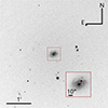 |
Fig. 1. Acquisition image of SN 2021efd and its host galaxy, taken with the NOT using ALFOSC without a filter on 4 April 2021 UT (MJD 59318.94). The red markers in the zoomed-in image mark the location of SN 2021efd in the host galaxy. |
The organization of this paper is as follows. Sect. 2 presents the observations. The photometric and spectroscopic properties are detailed in Sects. 3 and 4, respectively. Sect. 5 estimates the key properties of SN 2021efd. The origin of the brightness excess is examined in Sect. 6, along with the derivation of the CSM properties through LC modeling. Sect. 7 addresses the mass-loss mechanism that creates the CSM in SN 2021efd and its progenitor. The paper concludes with a summary in Sect. 8.
2. Observations and data reduction
2.1. Photometry
We present 40 epochs of multiband (uBVgri) photometry of SN 2021efd obtained with the Las Campanas Observatory’s (LCO) 1-m Henrietta Swope telescope equipped with a direct imaging camera. These data were obtained as part of the Precision Observations of Infant Supernova Explosions (POISE) collaboration (Burns et al. 2021) and extend from −12.6 to +27.2 days with three additional epochs between +390.6 and +392.1 days. Imaging data were reduced following standard procedures (Hamuy et al. 2006), and the instrumental magnitudes from the point-spread-function (PSF) photometry of the SN were calibrated to apparent magnitudes using nightly zero-points inferred from a local sequence of stars calibrated by standard star observations. The host galaxy flux was subtracted with a template photometry taken three years after the explosion.
We also present eight epochs of late-time gri photometry from the NOT using the Alhambra Faint Object Spectrograph and Camera (ALFOSC), two epochs of r photometry with the Palomar 60-inch telescope (P60) using SED Machine (SEDM, Blagorodnova et al. 2018), and one epoch of griz photometry with the 6.5-m Multi-Mirror Telescope (MMT) using the Binospec instrument. These data were obtained as part of the Zwicky Transient Facility collaboration. Photometry of ALFOSC and Binospec data was performed following the procedures as described in Chen et al. (2022). We used archival images from the Pan-STARRS1 (PS1) survey as reference images for image subtraction. The instrumental magnitudes were obtained with PSF photometry on the subtracted images. The photometric zero-point calibration was done using the reference stars in the field view of the science image.
Our photometry of SN 2021efd is complemented with measurements obtained by the ZTF survey (Bellm et al. 2019; Graham et al. 2019; Masci et al. 2019) and the ATLAS Project (Asteroid Terrestrial-impact Last Alert System; Tonry et al. 2018; Smith et al. 2020). Photometry from these public surveys were retrieved through the ZTF Forced Photometry Service1 (Masci et al. 2023) and the ATLAS Forced Photometry Service (Shingles et al. 2021)2, respectively. These photometric measurements were obtained on science images having undergone host-galaxy template subtraction. We adopted a signal-to-noise ratio of 3 as the detection limit for the forced photometry. The photometry from these surveys was binned into one-day intervals.
2.2. Spectroscopy
We present 13 epochs of optical spectroscopy of SN 2021efd extending from −12 days to +771 days. Four of these were obtained with the NOT equipped with ALFOSC as part of the NOT Unbiased Transient Survey (NUTS2) collaboration. A pre-maximum spectrum was also obtained by POISE with the 6.5-m Magellan Baade telescope equipped with the Inamori-Magellan Areal Camera and Spectrograph (IMACS). One nebular spectrum was obtained with the Very Large Telescope (VLT) equipped with the FOcal Reducer and low dispersion Spectrograph 2 (FORS2). Additionally, six nebular spectra were obtained by the ZTF collaboration with the Keck telescope using the Low Resolution Imaging Spectrograph (LRIS), and one with the MMT using the Binospec instrument. The nebular spectra span from +324 days until +771 days. A journal of spectroscopic observations is provided in Table 1.
Log of spectral observations of SN 2021efd.
Spectroscopic data were reduced following standard procedures, including bias subtraction, flat-field correction, spectral extraction, wavelength correction, and flux calibration relative to sensitivity functions derived from observations of spectroscopic flux standard stars. We reduced the spectroscopic data using the ALFOSCGUI3 and ESO pipelines for the ALFOSC and FORS spectra, respectively. The IMACS spectrum was reduced with standard IRAF procedures. For the Binospec spectrum, the basic data processing (bias subtraction, flat fielding) is done using the Binospec pipeline (Kansky et al. 2019). The spectrum is reduced with IRAF, including cosmic-ray removal, wavelength calibration (using arc lamp frames taken immediately after the target observation), and relative flux calibration with archived spectroscopic standards observation. The LRIS spectra (Oke et al. 1995) were reduced with Lpipe (Perley 2019). The nebular phase spectra and the IMACS spectrum were also corrected for telluric features. In the case of the IMACS spectrum, residuals of the telluric feature remain.
We obtained the nebular spectrum of SN 2019tsf at +418 days under the same program and setup as the FORS2 spectrum of SN 2021efd, except with an order blocking filter. This phase was not covered by the previous studies of SN 2019tsf (Sollerman et al. 2020; Zenati et al. 2022). Spectroscopic data are available for download in electronic format on WISeREP (Weizmann Interactive Supernova Data Repository)4.
3. Photometric properties
3.1. Estimating the explosion date
We estimate the explosion date by fitting the early phases of the LC with a power-law curve of f0(t − t0)n. Here, t0 is the explosion date, f0 is a scaling coefficient in flux units, and n is the power-law index. The r-band data for this analysis were used because of the comprehensive coverage of the early phases. The epochs chosen for the fitting are from −11 to −5 days before the peak. We estimate the explosion date to be MJD ≈59273.7 ± 1.2. This is 15.5 ± 1.2 days prior to the observed r-band peak. The last nondetection prior to discovery, obtained on MJD 59269.27 with a ZTF r-band limiting magnitude of > 21.35, occurred ∼4.4 days before this estimated explosion date.
3.2. Light-curve evolution
The multiband LCs of SN 2021efd are displayed in Fig. 2. The peak absolute g- and r-band magnitudes are Mg = −16.77 ± 0.02 mag and Mr = −17.31 ± 0.01 mag, where the error is the photometric error. The absolute magnitudes here are corrected for MW extinction, but no K-correction was applied. The late-time (≳300 days) photometric data points from the ZTF and ATLAS surveys are near the detection limits of these surveys, which is reflected by their large uncertainties. After the first peak, the LCs show rapid declines, which slow down at ∼30 days from the LC peak, as well as a rebrightening starting from ∼60 days. The LCs of SN 2021efd exhibit at least three clear peaks at +0, +75, and +105 days; these are visible in Fig. 3, where the LCs of all bands are overlaid. The magnitudes in this figure are shifted to match the second peak of the LCs at 75 days. The durations of these bumps are roughly 30 days; the bump at ∼105 days is more luminous than the one at ∼75 days. The late phases of the LC of SN 2021efd appear to have more bumpy features at ∼325 days, ∼345 days, ∼390 days, and ∼400 days that can not be clearly distinguished due to a low cadence of observations and large uncertainties. The strengths and durations of the latter bumps after ∼300 days can not be constrained with certainty since there is a lack of detailed observations during the possible bump and around it.
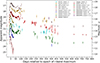 |
Fig. 2. Optical LCs of SN 2021efd corrected for MW extinction. The photometry obtained by POISE, ATLAS, and ZTF is plotted with triangles, squares, and circles, respectively. The unfilled triangles correspond to ZTF and ATLAS nondetections obtained prior to the first detections in each band. |
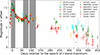 |
Fig. 3. Light curves of SN 2021efd with shifted magnitudes so that the second peaks match roughly. The shaded areas highlight the clear bumps at +0 days, ∼ + 75 days, and ∼ + 105 days. The dotted lines mark the possible later bumps at ∼ + 325 days, ∼ + 345 days, ∼ + 390 days, and ∼ + 400 days. |
We compare the r-band LC of SN 2021efd to those of other well-observed SESNe including the Type IIb SN 1993J (Richmond et al. 1994), the Type Ib iPTF13bvn (Srivastav et al. 2014), and the Type Ic SN 2007gr (Hunter et al. 2009) in Fig. 4. All of the LCs were corrected for extinction, which were determined in their respective articles. The first peak is similar to those of other SESNe, which are powered by the energy input from 56Ni. The rise time of SN 2021efd in the r band to the peak is 15.5 days (see Sect. 3.1), which is intermediate between the typical values for Type Ib and Type Ic SNe, i.e., slightly shorter than those for Type Ib and longer than those for Type Ic SNe (see Fig. 10 of Taddia et al. 2015). The decline rate after the first peak (Δm15 ∼ 0.57 mag for SN 2021efd from the POISE LC) is similar to the comparison SNe (0.83, 0.98, and 0.61 mag for SN 1993J, iPTF13bvn, and SN 2007gr, respectively). After ∼30 days from the r-band peak, its decline becomes slower, as if it enters the tail phase. The difference between the magnitudes at the peak and the beginning of the tail phase is smaller (Δm30 ∼ 0.86 mag for SN 2021efd) than those for the other SNe (1.37, 1.58, and 1.41 mag for SN 1993J, iPTF13bvn, and SN 2007gr, respectively). This may imply that an additional powering mechanism starts to contribute to the LC evolution around this time, in addition to the radioactive decay power by 56Ni and 56Co (see Sect. 6).
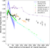 |
Fig. 4. Light curve of SN 2021efd compared to the LCs of other SESNe and templates of Type Ibn SNe from Hosseinzadeh et al. (2017). The comparison SNe include a regular Type Ib SN iPTF13bvn (Srivastav et al. 2014), a regular Type IIb SN 1993J (Richmond et al. 1994), a regular Type Ic SN 2007gr (Hunter et al. 2009), and a peculiar Type Ib SN 2019tsf (Masci et al. 2019). |
The r-band LC of SN 2021efd at late times bears no resemblance to regular SESNe. Around 30 days after the r-band peak, the LC deviates from the linear decline, and at around 60 days, the LC begins brightening again with two additional peaks at ∼75 and 105 days. At the beginning of the tail phase during the period from 20 to 50 days, the decline rate is 1.49 mag per 100 days, which is roughly consistent with the 1.33 mag per 100 days expected from radioactive decay of both 56Ni and 56Co with full γ-ray trapping (Arnett 1980, 1982). The decline rate at the tail phase is 0.60 mag per 100 days during the period from 50 to 200 days from the r-band peak. This value is less than that expected from 56Co decay, 0.98 mag per 100 days in the case of the full γ-ray trapping (Arnett 1980, 1982). SN 2019tsf, which has been interpreted to be a Type Ib SN interacting with H-poor CSM (e.g., Sollerman et al. 2020; Zenati et al. 2022), has a similar bumpy LC. Its LC has a faster decay rate than that of SN 2021efd. SN 2010mb, which is a Type Ic SNe interacting with H/He-poor CSM (Ben-Ami et al. 2014), exhibits a slower decline and brightness excess at earlier epochs compared to SN 2021efd. The averaged R-band LC of Type Ibn SNe has a much higher peak luminosity and a significantly higher decline rate than those of regular SESNe and SN 2021efd.
3.3. Color evolution
The color evolution of SN 2021efd is presented in Fig. 5. We took all the ZTF photometry epochs that have both g- and r-band observations within one day and interpolated the magnitudes at these epochs. Using these interpolated magnitudes, we derive the g − r color of SN 2021efd. At late times, colors from ALFOSC, Swope, and Binospec are also included. Every individual (g − r) color is derived using g and r photometry from the same instrument. The photometric data were corrected for MW extinction but not for that of the host galaxy. The color evolution of SN 2021efd around the first peak is similar to that of SN 2006ep and SN 2007hn, respectively, a Type Ib and a Type Ic. During the rebrightenings, the color becomes bluer at a similar rate, although this is uncertain due to the noisy color evolution observed in SN 2021efd. At ∼100 days, the uncertainties in the photometry of SN 2021efd become large, and the observation epochs on different bands do not always coincide. Once SN 2021efd re-emerged from behind the Sun at ∼200 days, it had evolved to become much bluer. We note that, since the values of the magnitudes at late phases should be dominated by the strong spectral emission lines, the interpretation of the color evolution is not straightforward.
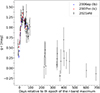 |
Fig. 5. g − r color evolution. The black dots show the evolution of SN 2021efd. The circles, diamonds, and pentagons correspond to ZTF, ALFOSC, and Binospec data, respectively. The blue line represents the color evolution of the Type Ib SN 2006ep, and the red line represents the Type Ic 2007hn presented in Stritzinger et al. (2018) |
3.4. Pseudo-bolometric light curve
We constructed a pseudo-bolometric LC of SN 2021efd by fitting its optical spectral energy distributions (SEDs) with single blackbody (BB) functions with both radius and temperature set as free parameters. The fitting was done using the linearly interpolated uBVcgroi data. We only used the epochs that had detections in three or more bands within 10 days (5 days before or after them). We determined the best fits using the χ2 goodness-of-fit test, and the errors represent the 1σ uncertainties. The results are displayed in Fig. 6. We note that, since the radiation at late phases does not exhibit a BB spectrum but is instead dominated by emission lines (see also Sect. 4), the inferred BB parameters at late phases should be considered reference values based on the assumption of BB radiation.
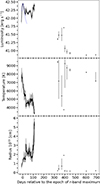 |
Fig. 6. Results of the BB fitting. Top: bolometric LC of SN 2021efd (black) and bolometric luminosity of Type Ib SN 2004gv (blue) (Taddia et al. 2018) indicated by a dotted blue line. Middle: BB temperature of the photosphere. Bottom: BB radius of the photosphere. The errors are the 1σ uncertainties of the χ2-fitting. Since the cadence after 115 days is poor, these observations were plotted separately. |
The pseudo-bolometric LC to first order follows the evolution of the LC in the single bands, also displaying multiple bumps and an overall slow decline. The peak luminosity during the first peak is ∼2.8 × 1042 erg. The total radiated energy derived from the pseudo-bolometric LC until ∼710 days is ∼4.9 × 1049 erg. The total generated energy from the decay of 56Ni and 56Co is 1.89 × 1050 × MNi/M⊙ erg (Arnett 1980, 1982) and MNi for SESNe ranges from ∼0.01 to 0.3 M⊙ (e.g., Taddia et al. 2018; Afsariardchi et al. 2021), thus the typical energy released in radioactive decay is ∼1048 − 1049 erg. Due to incomplete γ-ray trapping, not all of the released energy contributes to the observed luminosity.
The BB temperature evolution shows cooling until phase 25 days. The sudden drop in temperature happened at the time of the last observations with the Swope telescope (27 days), which is probably caused by the end of the coverage on the uBV bands. After this, the temperature appears to be roughly constant. Later, at ≳300 days from the r-band peak, SN 2021efd shows an increase in temperature, although at later epochs the error on the temperature is large. During the photospheric phase, the SN is well described by a BB function, but as the SN ejecta expands, the SN becomes emission-line dominated. At later epochs, this increases the BB fit uncertainties, especially in the calculated temperature, which is sensitive to the relative brightness in different bands. In addition to this, the cadence of the observations drops after ∼115 days. The BB fit at later phases ≳100 days may not reflect the actual physical characteristics of the SN, and the derived values are indicative.
The BB radius increases to ∼2 × 1015 cm toward the LC peak and remains roughly constant for ∼70 days. It slightly decreases to ∼1.5 × 1015 cm as the BB temperature increases at ∼80 days after the r-band peak. After the gap in observations, the radius is relatively stable at ∼2 × 1014 cm. From the initial rise of the BB-radius, we can roughly estimate a photospheric velocity of ∼6000 km s−1 measured from −12 days until −5 days.
4. Spectroscopic properties
4.1. Spectroscopic evolution
The early-phase spectra of SN 2021efd are displayed in Fig. 7. They were taken before the rebrightening, which begins at around 60 days. These spectra are typical of the early and near-maximum phases of Type Ib SNe with He I, Fe II, and Ca II lines being present. A weak Si II is also present, and a O I line starts forming at 7774 Å after the brightness peak. The narrow Hα-[N II] lines in the spectra likely originate from the host galaxy.
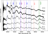 |
Fig. 7. Early-time spectra of SN 2021efd. The flux scale is arbitrary. The telluric features are marked with gray lines. The locations of some typical lines at zero velocities are indicated. |
The nebular spectra of SN 2021efd, displayed in Fig. 8, are dominated by emission lines, as is typical for SESNe. The [O I] doublet at ∼6300 Å, the O I line at 7774 Å, the [Ca II] doublet at ∼7200 Å, and the Ca II NIR triplet at ∼8500 Å are the most prominent features. Additionally, He lines are present at 4921 Å and 5876 Å. These coincide in wavelength with an Fe II and a Na I line, respectively, but as there are other prominent He I lines present, we consider the He I identification as more likely. The blue part is dominated by Fe II complex lines. At 4571 Å there is also a superposition of Mg I] and [Fe II]. In the nebular spectrum, prominent lines (e.g., O I, Ca II) have both broad and narrow (∼1000 km s−1) components, which is observed in other interacting SESNe as well (e.g., SN 2022xxf, Kuncarayakti et al. 2023). The time evolution of the lines in the nebular spectra is displayed in Fig. 9. Except for some small variation, the nebular lines remain mostly unchanged.
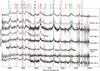 |
Fig. 8. Nebular phase spectra of SN 2021efd. The spectra are corrected for telluric features. The locations of some typical lines are indicated in the figure, even when they are not present. |
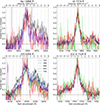 |
Fig. 9. Line profiles of the nebular spectra. Some epochs are excluded for clarity. The rest wavelength of what appears to be the strongest line is displayed as the zero point of velocity. |
4.2. Comparison of the spectra
The early-phase spectra of SN 2021efd are compared in Fig. 10 with those of the Type Ib iPTF13bvn (Cao et al. 2013), the Type IIb SN 1993J (Barbon et al. 1995), the Type Ic SN 2007gr (Valenti et al. 2008), the peculiar Type Ib SN 2019tsf (Sollerman et al. 2020), as well as with the Type Ibn SNe iPTF14aki (Hosseinzadeh et al. 2017) and 2010al (Pastorello et al. 2015). At early phases, SN 2021efd is similar to the typical Type Ib SNe. All the lines present in SN 2021efd are also present in iPTF13bvn. The other SESNe differ notably by their lack of helium in the case of SN 2007gr, or by the presence of hydrogen in SN 1993J. SN 1993J also has weaker Fe II lines in the blue part of the spectrum and a weaker Ca II NIR triplet absorption feature. Observationally SN 2021efd has no resemblance to Type Ibn SNe. The spectra of Type Ibn SNe are mostly continuum-dominated, with iPTF14aki showing a greater number of narrow lines in its spectra. The spectral features of SN 2019tsf are similar to those of SN 2021efd and iPTF13bvn, which is noteworthy as its LC decline rate at this epoch already suggests a contribution from another powering mechanism in addition to radioactive decay.
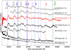 |
Fig. 10. Photospheric phase spectra of SN 2021efd and multiple other SESNe. Flux normalization was done by dividing the flux at every wavelength by the peak flux between 4200 and 5000 Å. The locations of some typical lines are indicated. |
The nebular-phase spectrum of SN 2021efd is compared in Fig. 11 to similar phase spectra of the comparison sample. These include SN 1993J (Jerkstrand et al. 2014), the Type Ib SN 2012au (Milisavljevic et al. 2013), SN 2007gr (Shivvers et al. 2019), SN 2019tsf and the interacting Type Ic SN 2010mb (Ben-Ami et al. 2014). The spectrum of SN 2021efd exhibits a narrow O Iλ7774 line similar to the one observed in SN 2019tsf. It can also be seen that the Ca II NIR triplet is much stronger in SN 2021efd than in the regular SESNe. Similar to SN 2019tsf, SN 2021efd has an excess of continuum flux around the iron complex (∼4000 − 5500 Å). This may suggest a similar powering mechanism of H-free CSI. Despite the lack of narrow lines in the spectrum of SN 2019tsf, they can not be ruled out due to the noisiness of the spectra. SN 2010mb also exhibits a blue excess and strong Ca II NIR lines.
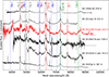 |
Fig. 11. Nebular phase spectra of SN 2021efd and several other SESNe. Flux normalization was done by dividing the flux at every wavelength with the peak flux of the [O I] line at ∼6300 Å. |
4.3. Velocity evolution
We calculate the velocity of the Fe IIλ5169 line and the He Iλ5876 line from their absorption minima by fitting the absorption features with a Gaussian function. The He I 5876 Å feature might have a contribution from Na Iλλ5890, 5896. In Fig. 12, we compare the spectral line evolution of these features along with those measured from the SESN sample published by the Carnegie Supernova Project (Stritzinger et al. 2023; Holmbo et al. 2023). The ejecta velocity of SN 2021efd inferred from both the He I and Fe II lines in the spectra at the early epochs is in the range of what is typical for SESNe (Fig. 12). While the He I velocity is around the higher end for an SESN, the Fe II velocity is at the lower end, though both velocities are still within the distributions. The velocity inferred from the early-time evolution of the BB radius (∼6000 km s−1; see Sect. 3) is roughly in line with the Fe II velocity measured from the spectra (∼8000 km s−1 around the brightness peak).
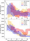 |
Fig. 12. Top: He Iλ5876 velocity of SN 2021efd. Bottom: Fe IIλ5169 velocity of SN 2021efd. The templates are the rolling mean of SESNe as presented by Holmbo et al. (2023); H23. The λ5876 feature they measured for Type Ic SNe is expected to be composed of Na Iλλ5890,5896 doublet, and little to no He Iλ5876. |
4.4. [O I]/[Ca II] line ratio
We measured the fluxes of the [O I] λλ6300, 6364 and the [Ca II] λλ7292, 7324 doublets. We determine a continuum level and then subtract the nearby Fe II and N II lines by assuming a symmetric profile, as done in Fang et al. 2022. The [O I] to [Ca II] ratio of SN 2021efd is 1.3–1.4 during the epochs from 324 days to 473 days. At 641 days and at 771 days, the ratio is 1.7. The measurement of the [O I] to [Ca II] ratio might be affected by uncertainties from the nearby lines, in particular their possible asymmetry due to the assumption of the symmetric profiles of Fe II and N II. It has been found that Type IIb and Type Ib SNe have similar [O I]/[Ca II] flux ratios, while Type Ic SNe typically have higher values, although overlapping with SNe IIb/Ib (Fang et al. 2022). Compared to the values reported in Fig. 3 of Fang et al. (2019), SN 2021efd sits in the overlapping region of SESNe.
5. Supernova ejecta properties
We estimate the ejecta properties of SN 2021efd, such as the mass, kinetic energy, and 56Ni mass of the ejecta, under the assumption that the CSM interaction has a minimal contribution to the SN brightness before and around the first LC peak. This assumption is supported by the fact that the early-phase photometric and spectroscopic properties of SN 2021efd are similar to those of the other noninteracting, SESNe.
For the estimation of the mass and kinetic energy of the ejecta, we use the following equations in the one-zone analytic model for the LCs from the homologously expanding gas with radiative diffusion (Arnett 1982, 1996),
where β is an integration constant equal to 13.8, κ is the opacity of the ejecta gas, vph is the ejecta velocity, and tmax is the rise time of the LC. Here, κ is assumed to be 0.1 cm2 g−1, which is typical for ionized H-poor gas, although it can vary depending on the chemical composition of the gas. We assume the ejecta velocity to be 8300 km s−1, which is the velocity inferred from the Fe IIλ5169 line around the LC peak, and the rise time to be 18.5 days, which is the value estimated from the pseudo-bolometric LC. We find the ejecta mass to be 2.2 ± 0.3 M⊙ and the kinetic energy of the ejecta to be 9.1 ± 1.2 × 1050 erg, where the uncertainty is due to the error of the rise time.
We estimate the 56Ni mass from its relation with the peak luminosity (Arnett 1980, 1982),

This gives an estimate of 0.14 ± 0.01 M⊙, where the error is calculated using the limits from the bolometric luminosity fit. This method is known to overestimate the 56Ni mass by a factor of ∼2 (Afsariardchi et al. 2021). In addition, since the peak luminosity of SN 2021efd might be enhanced by the contribution of potential interaction with CSM, the actual 56Ni mass can be smaller than this estimated value. The total energy released by the radioactive decay of this amount of 56Ni is (2.6 ± 0.2)×1049 erg, which is smaller than the total energy radiated by SN 2021efd (4.9 × 1049 erg) until 710 days, as measured by integrating the entire pseudo-bolometric LC.
We compare these derived values of the ejecta mass, kinetic energy, and 56Ni mass for SN 2021efd to those of other SESNe. Taddia et al. (2018), who followed a similar approach in their work, found the average values for Type Ib SNe to be Mej = 3.9 ± 2.7 M⊙, Ek = 1.6 ± 1.0 × 1051 erg, and MNi = 0.10 ± 0.05 M⊙ respectively. For Type Ic, they estimated Mej = 2.5 ± 1.2 M⊙, Ek = 1.2 ± 0.8 × 1051 erg, and MNi = 0.14 ± 0.04 M⊙. The errors here are the standard deviations of the sample. The values that we derived for SN 2021efd (Mej = 2.2 ± 0.3 M⊙, Ek = 0.91 ± 0.12 × 1051 erg, and MNi = 0.14 ± 0.01 M⊙) are consistent with these average values for Type Ib and Type Ic SNe within the standard deviation. While SN 2021efd has slightly lower ejecta mass and kinetic energy than the average values, its 56Ni mass is slightly higher than the average value for Type Ib SNe and similar to the average value for Type Ic SNe.
6. Origin of the late-time excess and the CSM properties
In this section, we discuss the origin of the late-time excess in the brightness of SN 2021efd and derive its CSM properties with LC modeling. Several possible scenarios for the late-phase rebrightening in SESNe (e.g., Moore et al. 2023; Kuncarayakti et al. 2023; Chen et al. 2024; Kangas et al. 2024) have been proposed. These include: delayed CSM interaction (e.g., Chevalier & Fransson 2006), delayed activity of a newly formed magnetar (e.g., Kasen & Bildsten 2010), or delayed accretion onto a newly formed compact object (e.g., Dexter & Kasen 2013). In the case of SN 2021efd, the LC shows clear bumps at ∼75 and ∼100 days from the explosion, and possibly at 325, 345, 390, and 400 days as well. With either the magnetar or fall-back accretion scenarios, it is difficult to explain not only the delayed onsets of the rebrightenings but also the multiple onsets (e.g., Kasen & Bildsten 2010; Dexter & Kasen 2013). The multiple bumps in the LC favor the CSM interaction scenario, where the bumps are created by interactions with multiple shell-like or clumpy CSM. At the same time, since its early-time photometric and spectroscopic properties are similar to those of prototypical Type Ib SNe (see Sects. 3 and 4), it might be natural to consider the cause of the rebrightenings as not the difference of the SN ejecta or progenitors (e.g., as in the magnetar or fall-back accretion scenarios) but the difference of some external factor (e.g., as in the CSM interaction scenario). Furthermore, the features in the late-time spectrum (i.e., the spectra from phase 315 days onward; see Fig. 8) support the CSM interaction scenario. The narrow emission lines with velocities of ∼1000 km s−1 point to slower-moving material than the bulk SN ejecta, consistent with the CSM interaction scenario. A similar velocity scale was observed in post-maximum near-infrared spectra of Type Ic SN 2016adj, which also showed signatures of interaction with H-rich gas (Stritzinger et al. 2024). The so-called Fe bump near ∼5200 Å, likely created by highly ionized and/or excited Fe lines, is frequently seen in interacting SNe of various types, including Type IIn, Ia-CSM, interacting Ibc, Ibn, and Icn (e.g., Sharma et al. 2023; Kuncarayakti et al. 2018b; Pastorello et al. 2008; Pellegrino et al. 2022). Therefore, we conclude that the late-time LC bumps in SN 2021efd are due to interaction with multiple-shell, multiple-ring, or clumpy CSM.
6.1. Light-curve model
In order to derive the properties of the CSM in SN 2021efd, we analyzed the bolometric LC using the luminosity model presented in Moriya et al. (2013b). The strong interaction between the SN ejecta and CSM creates a shock shell, in which the kinetic energy of some parts of the ejecta is transformed into radiation energy. For calculating the radiation from the CSM interaction, we assess the evolution of the shock shell. We assume that the parameters within the shock shell are uniform, and the width of the shock shell is negligible in comparison to its extent. As in Moriya et al. (2013b), we derive the time evolution of the location (rsh) and velocity (vsh) of the interaction shock shell using its equation of motion,
![Mathematical equation: $$ \begin{aligned} M_{\mathrm{sh}} \frac{\mathrm{d} v_{\mathrm{sh}}}{\mathrm{d} t} = 4 \pi r_{\mathrm{sh}}^2\left[\rho _{\mathrm{ej}}\left(v_{\mathrm{ej}}-v_{\mathrm{sh}}\right)^2-\rho _{\mathrm{csm}}\left(v_{\mathrm{sh}}-v_{\mathrm{csm}}\right)^2\right], \end{aligned} $$](/articles/aa/full_html/2026/02/aa57292-25/aa57292-25-eq3.gif) (1)
(1)
where ρ and v are density and velocity, respectively, and the subscripts of ej, sh, and csm correspond to the ejecta, shock shell, and CSM, respectively. Msh is the total mass of the shock shell, i.e., the shocked CSM and ejecta. We assume that the CSM velocity is constant, and that the ejecta is homologously expanding:  . We use the density profiles of the ejecta that are estimated based on numerical simulations (Matzner & McKee 1999), that is, the double power-law distribution of Moriya et al. (2013b),
![Mathematical equation: $$ \begin{aligned} \rho _{\mathrm{ej} }\left(v_{\mathrm{ej}}, t\right) = {\left\{ \begin{array}{ll}\frac{1}{4 \pi (n-\delta )} \frac{\left[2(5-\delta )(n-5) E_{\mathrm{ej}}\right]^{(n-3) / 2}}{\left[(3-\delta )(n-3) M_{\mathrm{ej}}\right]^{(n-5) / 2}} t^{-3} v_{\mathrm{ej}}^{-n}&\left(v_{\mathrm{ej}}>v_t\right), \\ \frac{1}{4 \pi (n-\delta )} \frac{\left[2(5-\delta )(n-5) E_{\mathrm{ej}}\right]^{(\delta -3) / 2}}{\left[(3-\delta )(n-3) M_{\mathrm{ej}}\right]^{[\delta -5) / 2}} t^{-3} v_{\mathrm{ej}}^{-\delta }&\left(v_{\mathrm{ej}} < v_t\right),\end{array}\right.} \end{aligned} $$](/articles/aa/full_html/2026/02/aa57292-25/aa57292-25-eq5.gif) (2)
(2)
where δ and n are the outer and inner density slopes, respectively. Mej and Eej are the mass and energy of the ejecta, respectively, and vt is the velocity at the border of the power laws,
![Mathematical equation: $$ \begin{aligned} v_t=\left[\frac{2(5-\delta )(n-5) E_{\mathrm{cj}}}{(3-\delta )(n-3) M_{\mathrm{ej}}}\right]^{\frac{1}{2}}. \end{aligned} $$](/articles/aa/full_html/2026/02/aa57292-25/aa57292-25-eq6.gif) (3)
(3)
For the mass and energy of the ejecta, we adopt the values estimated in Sect. 5: Mej = 2.2 ± 0.3 M⊙ and Eej = 9.1 ± 1.2 × 1050 erg. We adopt the values n = 10 and δ = 1 (e.g., Matzner & McKee 1999; Kasen 2010; Moriya et al. 2013b).
We assume the rate of the mass loss from the progenitor system (Ṁ) is constant in time, and thus the density of the CSM at distance r is written as
 (4)
(4)
Here, we define D as Ṁ/(4π vcsm). Since we do not know the mechanism of the mass loss, the expansion velocity of the CSM (vcsm) is unclear. We estimate the CSM velocity to be ∼100 − 1000 km s−1 (see Sect. 7.2). Here, we simply use the minimum value of vcsm = 100 km s−1, which produces the minimum value of the necessary mass-loss rate, as a fiducial value, and also discuss the case with the maximum value of vcsm = 1000 km s−1.
By numerically solving the equation of motion with the ejecta and CSM parameters assumed above, we calculate the distance and velocity of the shock shell as a function of time. We assume the optically thin limit, where a fraction of the generated energy ( ) immediately escapes from the shocked shell as optical radiation, and calculate the optical luminosity as follows (Moriya et al. 2013b):
 (5)
(5)
The value ϵ is the conversion efficiency from the kinetic energy of the SN ejecta into the optical radiation due to the CSM interaction. We assume the value of ϵ to be 0.1 (Moriya et al. 2013a).
6.2. Comparison with the observation
The bolometric LC of SN 2021efd is compared to the calculated interaction luminosity in Fig. 13. The radioactive-decay component is subtracted using the analytical formula presented in Arnett (1980, 1982) and assuming the 56Ni mass to be 0.14 M⊙. Since this formula assumes full γ-ray trapping, the later parts of this radioactive-decay LC are likely overestimated. The actual interaction component is thus expected to be somewhere between the LC without the radioactive component and the original bolometric LC. After ∼60 days from the explosion onward, the interaction luminosity is increasing. This could be due to an increase in the corresponding mass-loss rate for the encountered CSM, suggesting the presence of an inner cavity in the CSM distribution. The early parts (at least from ∼80 to ∼120 days) can be roughly explained by the LC models with ∼5 × 10⁻³ − ∼10−2 M⊙ yr−1. The later parts (at least after ∼340 days) are significantly lower than these levels, which suggests that the mass-loss rate of the progenitor of SN 2021efd is not constant, but grows with time toward the explosion.
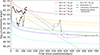 |
Fig. 13. Comparison of the bolometric LC of SN 2021efd with the models. The colored lines are the calculated luminosities from interaction based on the model. The black line is the bolometric luminosity of SN 2021efd with the radioactive decay component subtracted. The dashed line is the observed bolometric LC, and the dotted line is the radioactive decay component calculated from peak luminosity. |
Here, we note a caveat on the estimated mass-loss rate. The CSM velocity is directly proportional to the mass-loss rate, as can be seen from Eq. 4. CSM velocities of 1000–2000 km s−1 have been found for Type Ibn SNe, and have been suggested for WR stars (e.g., Hosseinzadeh et al. 2017; Crowther 2007). A velocity of 1000 km s−1 would increase the estimated mass-loss rate by an order of magnitude, to 10−1 M⊙ yr−1. Since we cannot estimate the precise CSM velocity in the case of SN 2021efd, the estimated mass-loss rate is a lower limit. The uncertainty of the value of the efficiency ϵ, which is directly proportional to the luminosity, does not largely affect the estimated value. In fact, even a change of the assumed ϵ value by a factor of two, i.e., ϵ = 0.05 − 0.2, does not change the order of magnitude of the estimate, as this is equivalent to adding or subtracting log10(L) by log10(2) = 0.3 (see Fig. 13).
Figure 14 displays the accumulated mass of the shock shell over time. From this figure, we can see that the masses for the good-fit models already reach a few times 10−1 M⊙ at ∼120 days. This is the lowest limit of the actual total CSM mass, as in the observed LCs we can see excessive flux until at least ∼770 days and possibly later as well (see Fig. 2).
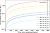 |
Fig. 14. Mass of the shock shell accumulated from the CSM at each epoch according to the values used in the calculated interaction luminosity. Effectively, this tells us the CSM mass up to a certain distance from the progenitor star. |
6.3. Geometry of the CSM
Here we discuss the geometry of the CSM, which is directly related to the mass-loss mechanism. We have concluded that the late-time rebrightenings in SN 2021efd are due to interaction with CSM with a multiple-shell/ring-like or clumpy structure. The LC modeling demonstrates that mass loss with an average rate of Ṁ ∼ 10−2 M⊙ yr−1 can explain the overall luminosity of the bolometric LC. Here, the best-fit model predicts the velocity of the interaction shock as ∼6000 km s−1, while the narrow allowed lines in the nebular spectra (OI, Ca II, Mg II, and He I; see Fig. 9), which should originate from the gas in the shock shell, and not from the unshocked ejecta, indicate that some interaction regions of the SN ejecta were decelerated to ∼1000 km s−1. This discrepancy suggests that the actual CSM must be confined to smaller regions and thus denser than the spherical CSM assumed in the LC modeling. At the same time, the coexistence of the narrow and broad components of the ejecta emission lines in the nebular spectra of SN 2021efd further supports a clumpy distribution for the CSM rather than a distribution with multiple rings of different sizes on a single orbital plane. This spectral feature requires multiple emitting regions at different locations of the ejecta, while, in the multiple-ring scenario, the interaction – and thus the energy input – occurs at a specific radius at a given time. A schematic representation of the inferred CSM geometry is shown in Fig. 15.
 |
Fig. 15. Schematic of the preferred model in the nebular phase. Arrows are used to mark characteristic regions for the narrow and broad components, respectively. The light blue coloring approximately corresponds to the shock regions. |
7. Discussion
7.1. Progenitor system of SN 2021efd
In this subsection, we discuss the potential progenitor of SN 2021efd. As shown in Sect. 5, the estimated ejecta properties of SN 2021efd (the velocity, mass, kinetic energy, and Ni mass) are within the diversity of typical Type Ib and Ic SNe. This might suggest that the progenitor star of SN 2021efd is similar to those of typical Type Ib and Ic SNe, whose ZAMS masses are likely ≲20 M⊙ (e.g., Bersten et al. 2014; Yoon et al. 2017; Dessart et al. 2024).
Another hint for estimating the properties of the progenitor is the [O I]/[Ca II] ratio in the nebular spectra, which is often used as a measure of the ZAMS core masses of the SN progenitors. We compare the [O I] to [Ca II] ratios of SN 2021efd, which are estimated to be ∼1.3 from the spectra between phases from 324 days to 476 days and ∼1.7 from the spectra at 641 days and 771 days (see Sect. 4.4), to those from the simulated spectra of SESNe in Dessart et al. (2023). These spectra are calculated with different initial conditions, including the mass of the He star. We measure the [O I] to [Ca II] ratios of these synthesised spectra as for the nebular spectrum of SN 2021efd. The results are plotted in Fig. 16. The [O I] to [Ca II] ratio of SN 2021efd is closest to that for the model with He star mass of 7 M⊙, which corresponds to a ZAMS mass of ∼25 M⊙ (Dessart et al. 2023; Woosley 2019; Ertl et al. 2020). Here, we note that in SN 2021efd, the dominant energy input at late phases is not the 56Co decay in the inner ejecta, but rather the CSM interaction in the outer ejecta, which might affect the [O I]/[Ca II] ratio. Therefore, this progenitor mass measurement should be considered as a reference. Although this estimate is not necessarily correct, the estimated ZAMS mass of ∼25 M⊙ for SN 2021efd is roughly comparable to those for typical Type Ib and Ic SNe. The progenitors of Type Ic SNe are typically expected to have slightly greater ZAMS masses than those of Type Ib SNe. Depending on metallicity, a ZAMS mass of ∼25 M⊙ is compatible with progenitors of both Type Ib and Type Ic SNe based on, for example, theoretical predictions from stellar evolution models (Georgy et al. 2009), and population studies of SN environments (Kuncarayakti et al. 2018a).
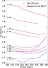 |
Fig. 16. [[O I]/[Ca II] ratio of models with different He star masses measured from synthetic spectra presented by Dessart et al. (2023). The different lines correspond to different He star masses of the models. The black dots are the values measured from the nebular spectra of SN 2021efd (see Sect. 4.4). |
7.2. Mass-loss properties
The CSM properties inferred in Sect. 6 suggest that the final mass-loss processes of the progenitor of SN 2021efd before the explosion were accompanied by episodic mass ejections with mass-loss rates of Ṁ ≲ 10−2 M⊙ yr−1. The velocity of the CSM is uncertain. Theoretically, different mechanisms would predict different CSM velocities. The minimum value of ∼100 km s−1 might be achieved in cases where the mass loss happens at a large distance from the progenitor star, such as the mass loss via the Roche-lobe overflow in a binary system, while the maximum value of ∼2000 km s−1 can be realized in cases such as mass ejections from the surface of H poor massive stars (e.g., Crowther 2007). Here, we have an observational hint for the velocity from the nebular spectra. As discussed in Sect. 6.3, the narrow lines from allowed transitions in the nebular spectra (O I, Ca II, Mg II, and S II), which have widths of ∼1000 km s−1, should originate from the gas in the shock shell. This indicates that some interaction regions should be decelerated to ∼1000 km s−1, and thus that the CSM velocity should be lower than this velocity. Therefore, we adopt 100 and 1000 km s−1 as the minimum and maximum values of the mass-loss velocity, respectively. In the following discussions, we use the minimum value of vcsm = 100 km s−1, which produces the minimum value of the necessary mass-loss rate, as a fiducial value, and also discuss the case with the maximum value assuming vcsm = 1000 km s−1.
The timescale of the mass ejections is estimated from the distances of the CSM clumps to the progenitor star. For simplicity, a characteristic velocity of 10 000 km s−1 is adopted for the outer ejecta. Since the peaks of the first and second rebrightenings are at ∼90 and ∼120 days after the explosion, respectively, we can estimate the distances of the CSM clumps that are responsible for these rebrightenings to be 8 × 10¹⁵ and 1 × 1016 cm. Such CSM clumps would have been ejected at ∼25 and ∼32 years before the SN explosion, assuming the CSM velocity of 100 km s−1. If the CSM velocity is 1000 km s−1, these values would instead be ∼2.5 and ∼3.2 years before the explosion. The duration of ∼30 days for these rebrightenings corresponds to the time duration of the mass ejections to be ∼0.8 − 8 years, depending on the assumed CSM velocity. The first and second rebrightenings correspond to mass-loss rates of approximately ∼5 × 10⁻³ − ∼10−2 M⊙ yr−1 with durations of about 8 years, assuming a CSM velocity of 100 km s−1. In contrast, for a CSM velocity of 1000 km s−1, the corresponding mass-loss rates are higher by a factor of ten, while the durations are shorter by a factor of ten. Regardless of the assumed CSM velocity, the masses of these CSM clumps were therefore estimated to be about 0.04 − 0.2 M⊙. The CSM interaction continues at least until ∼770 days after the explosion, which is the epoch of the last photometric detection. Thus, the extensive mass loss would have lasted at least from ∼220 to ∼12 years before the explosion with the assumption of vcsm = 100 km s−1 (from ∼22 to ∼1.2 years with the assumption of vcsm = 1000 km s−1). It is likely that this extensive mass loss would have been ongoing even before this period, simply because our last photometric observation does not suggest a decline. It might also be possible that there were minor mass ejections even after this period until the explosion, whose signs would have been hidden by the SN component of SN 2021efd.
7.3. Mass-loss mechanism
In this subsection, we discuss possible mass-loss mechanisms to create the CSM estimated for SN 2021efd based on its derived properties. Combining constraints on the progenitor and CSM properties, the progenitor of SN 2021efd was likely a He star, similar to those of typical Type Ib SNe, originating from stars with ZAMS masses of ≲25 M⊙ (e.g., Yoon et al. 2017; Dessart et al. 2024). In addition, the progenitor system should have a mass loss rate of 10−2 M⊙ yr−1 at least from ∼130 to ∼25 years before the explosion with the assumption of vcsm = 100 km s−1 (0.1 M⊙ yr−1 from ∼13 to ∼2.5 years with the assumption of vcsm = 1000 km s−1), which is much larger than the typical mass loss from massive stars including He stars (e.g., Smith 2014). This implies some extensive unknown type of mass ejections in a similar He star to the progenitors of typical Type Ib SNe, which we have rarely observed. If this extensive mass loss had lasted for a few thousands of years before the explosion in the scenario with vcsm = 100 km s−1 (a few hundred years for the scenario with vcsm = 1000 km s−1), the progenitor star would have become a carbon-oxygen-rich massive star, which would have exploded as a Type Ic SN. Given that the properties of SN 2021efd are similar to those of typical Type Ib and Type Ic SNe, the progenitor of SN 2021efd might have been a He star that was indeed on the way to becoming a potential progenitor of a Type Ic SN, but ended up as a Type Ib SN because of the timing of the explosion or late initiation of the mass loss. Thus, it is important to study the mass-loss mechanism in objects like SN 2021efd for a better understanding of the He-layer stripping in the progenitors of Type Ic SNe.
The first thing that we can say about the mass-loss mechanism is that the CSM appears to originate from the progenitor star. Since the CSM should be H-poor gas, it is natural to consider that the CSM gas should originate from the He star progenitor rather than from the potential companion star. If we consider the companion star as the origin of the CSM, it should be an H-poor star. In this case, since the main mechanism for the H-layer stripping is likely due to binary interaction (e.g., Yoon et al. 2017), the original H-rich gas of the companion star should transfer into the primary star, and the primary star should become a H-rich star. This is contradicted by the fact that the primary star exploded as a Type Ib SN, however. Thus, the H-poor CSM should originate from the He star progenitor that exploded as the Type Ib SN 2021efd.
One possible mechanism to remove the outer parts of the progenitor might be binary interaction, where the primary He star fills the Roche potential and transfers its gas into the companion star (e.g., Podsiadlowski et al. 1992; Yoon et al. 2010). The expected properties of the CSM in the binary interaction scenario do not match those inferred for SN 2021efd, however. The expected mass-loss rate in the binary scenario (≲10−4 M⊙ yr−1; Ercolino et al. 2025) is much smaller than that estimated for SN 2021efd (≳10−2 M⊙ yr−1; see Sect. 6). In addition, it is difficult to create not only episodic mass ejections with a period of ≲10 years (e.g., Ouchi & Maeda 2017) but also clumpy mass ejections accompanied by the CSM clumps (e.g., Vetter et al. 2024). The He layer stripping is therefore probably due to some mass ejections caused by the He star itself.
The mass ejections might be triggered by some instability related to the last burning phases in the massive-star evolution, which might be similar to the phenomenon that causes the confined CSM observed in Type II SNe (e.g., Khazov et al. 2016; Yaron et al. 2017; Boian & Groh 2020; Bruch et al. 2021). For this scenario, the rarity of the SN 2021efd-like events, that is, Type Ib SNe interacting with massive clumpy CSM (so far SNe 2019tsf and 2021efd), might be problematic. In addition, the CSM mass estimated for SN 2021efd is close to the upper end of those of the confined CSM of Type II SNe (≲1 M⊙; e.g., Förster et al. 2018), and its extension is larger than the confined CSM (≲1015 cm; e.g., Yaron et al. 2017), although it is more difficult to remove the mass from a H-poor star than the H-rich progenitors of Type II SNe. It might be natural to interpret that the progenitor of SN 2021efd was in an unstable state caused by another reason.
SN 2021efd might be related to other types of SNe. If the active mass-loss episode observed in SN 2021efd had occurred much earlier, the SN could have appeared as a regular Type Ib SN or Type Ic SN, depending on how much He remained at the surface. Conversely, if the mass-loss episode had started slightly earlier and lasted longer until the explosion, the SN might appear as a Type Ic SN interacting with H-poor CSM. In fact, some Type Ic SNe interacting with massive H-poor CSM show similar observational properties (e.g., SN 2010mb; Ben-Ami et al. 2014, SN 2021ocs; Kuncarayakti et al. 2022, SN 2022xxf; Kuncarayakti et al. 2023). These transients might be related to each other. The clumpy distribution and high mass-loss rate of the CSM in SN 2021efd resemble the giant eruptions of luminous blue variables (LBVs), although they are considered to be H-rich stars (e.g., Smith et al. 2011b). The mass-loss mechanism in SN 2021efd might be related to that for LBVs, although it is also under debate (e.g., Smith et al. 2011b).
Another speculative origin might be a merged He-rich star that has a peculiar ratio between the core and the envelope, creating an unstable state. Depending on the parameters of the original merging stars and the timing of the merger to the explosion, such merged stars might explode as Type IIL or Type IIn SNe (explosions of LBVs), normal Type Ib or Type Ic SNe, SN 2021efd-like events, or Type Ic-CSM SNe.
SN 2019tsf has a lot of similarities with SN 2021efd. When it appeared from solar conjunction, it had a similar r-band absolute magnitude to SN 2021efd at peak. Unlike SN 2021efd, it does not show a decay rate similar to regular SESNe at first, which may mean that it is already at a later epoch, or that the CSM was in closer proximity to the progenitor. In the multiband LC presented in Fig. 2 of Zenati et al. (2022), it has at least two additional bumps after the first detection, which was already after the first peak. The spectrum at the nebular phase is similar and shows the excess at the blue end like SN 2021efd, but no narrow lines are present in SN 2019tsf. Overall, we consider that SN 2019tsf might come from a similar progenitor system as SN 2021efd. One potential avenue to understanding the mass-loss histories of systems like these might be radio and X-ray observations.
8. Conclusion
We have performed an in-depth analysis of the peculiar Type Ib SN 2021efd. The photometric and spectroscopic properties of this object are typical of a Type Ib SN until ∼30 days after the epoch of maximum light. After this epoch, the LC of SN 2021efd began to show a higher luminosity until the end of the LC at ∼770 days, with at least two clear peaks at ∼75 and ∼105 days from maximum light. The early spectra of SN 2021efd are not significantly different from those of typical Type Ib SNe. The velocities of Fe IIλ5169 and He Iλ5876 in the early-phase spectra are consistent with those seen in other SESNe. The spectra of the nebular phase (≳300 days), however, contain features that are common in interacting SNe. There is an excess in the blue continuum, and almost all of the lines in the nebular spectra have a narrow and a broad component. The narrow components are ∼1000 km s−1 wide and probably originate from the shocked regions (allowed lines) and the SN ejecta around the shocked regions (forbidden lines). No signatures of hydrogen are detected at any epoch. The observational features of SN 2021efd resemble those of SN 2019tsf, suggesting comparable progenitor systems.
The derived ejecta and CSM properties are as follows: SN 2021efd has an ejecta mass of Mej = 2.2 ± 0.3 M⊙, a kinetic energy of Ek = (0.91 ± 0.12)×1051 erg, and a 56Ni mass of MNi = 0.14 ± 0.01 M⊙. The estimated progenitor mass of SN 2021efd from the [O I]/[Ca II] ratio is ∼25 M⊙, although this value is uncertain because we omitted the effects of CSI on the ratio. As for the CSM features, the estimated mass-loss rate of the progenitor is roughly ∼5 × 10⁻³ − 10−2 M⊙ yr−1 for the last few decades (∼8 − 32 years, depending on the assumed CSM velocity) and slightly lower before this final phase. The minimum CSM mass estimated by the photometric observations is a few times 10−1 M⊙. The observational properties suggest a clumpy CSM distribution.
The derived CSM properties contain important information on the He-layer stripping mechanism of Type Ic SNe progenitors. If this extensive mass loss had continued for a longer time than the actual case before the explosion, the progenitor of SN 2021efd could have lost more helium and become a carbon-oxygen-rich star that exploded as a Type Ic SN. The ejecta properties of SN 2021efd are similar to those of both Type Ib and Ic SNe, and its progenitor was therefore likely a He star in transition toward becoming a Type Ic SN. The study of this mass-loss process using our derived CSM properties provides insight into how He-layers are stripped in progenitors of Type Ic SNe.
Data availability
The photometric data presented in Fig. 2, all the spectra of SN 2021efd, the nebular phase spectrum of SN 2019tsf, and the result of the bolometric fit presented in Fig. 6 are available at the CDS via https://cdsarc.cds.unistra.fr/viz-bin/cat/J/A+A/706/A183. All spectra of SN 2021efd and the previously unpublished nebular spectrum of SN 2019tsf will also be available at WISeREP.
Acknowledgments
We thank Qiliang Fang, Anders Jerkstrand, and Stan Barmentloo for helpful discussions. We thank the anonymous referee for helpful comments. NP, TN, and HK acknowledge support via the Research Council of Finland (grant 340613). H.K. and T.N. were funded by the Research Council of Finland projects 324504, 328898, 353019, and 340613. M.D. Stritzinger and S. Bose are funded by the Independent Research Fund Denmark (IRFD, grant number 10.46540/2032-00022B) and by an Aarhus University Research Foundation Nova project (AUFF-E-2023-9-28). T.K. acknowledges support from the Research Council of Finland project 360274. Based on observations made with the Nordic Optical Telescope (NOT), owned in collaboration by the University of Turku and Aarhus University, and operated jointly by Aarhus University, the University of Turku and the University of Oslo, representing Denmark, Finland and Norway, the University of Iceland and Stockholm University at the Observatorio del Roque de los Muchachos, La Palma, Spain, of the Instituto de Astrofisica de Canarias. The NOT data were obtained under program ID P62-505. Based on observations collected at the European Organisation for Astronomical Research in the Southern Hemisphere under ESO programs 105.20DF.001 and 108.2282.001 (PI: Kuncarayakti). This work has made use of data from the Asteroid Terrestrial-impact Last Alert System (ATLAS) project. The Asteroid Terrestrial-impact Last Alert System (ATLAS) project is primarily funded to search for near earth asteroids through NASA grants NN12AR55G, 80NSSC18K0284, and 80NSSC18K1575; byproducts of the NEO search include images and catalogs from the survey area. This work was partially funded by Kepler/K2 grant J1944/80NSSC19K0112 and HST GO-15889, and STFC grants ST/T000198/1 and ST/S006109/1. The ATLAS science products have been made possible through the contributions of the University of Hawaii Institute for Astronomy, the Queen’s University Belfast, the Space Telescope Science Institute, the South African Astronomical Observatory, and The Millennium Institute of Astrophysics (MAS), Chile. Based on observations obtained with the Samuel Oschin Telescope 48-inch and the 60-inch Telescope at the Palomar Observatory as part of the Zwicky Transient Facility project. ZTF is supported by the National Science Foundation under Grant No. AST-2034437 and a collaboration including Caltech, IPAC, the Weizmann Institute of Science, the Oskar Klein Center at Stockholm University, the University of Maryland, Deutsches Elektronen-Synchrotron and Humboldt University, the TANGO Consortium of Taiwan, the University of Wisconsin at Milwaukee, Trinity College Dublin, Lawrence Livermore National Laboratories, IN2P3, University of Warwick, Ruhr University Bochum, Cornell University, and Northwestern University. Operations are conducted by COO, IPAC, and UW. The ZTF forced-photometry service was funded under the Heising-Simons Foundation grant #12540303 (PI: Graham). The Gordon and Betty Moore Foundation, through both the Data-Driven Investigator Program and a dedicated grant, provided critical funding for SkyPortal. SED Machine is based upon work supported by the National Science Foundation under Grant No. 1106171 Zwicky Transient Facility access was supported by Northwestern University and the Center for Interdisciplinary Exploration and Research in Astrophysics (CIERA). This research has made use of the Spanish Virtual Observatory (https://svo.cab.inta-csic.es) project funded by MCIN/AEI/10.13039/501100011033/ through grant PID2020-112949GB-I00. IS is supported by the PRIN-INAF 2022 project “Shedding light on the nature of gap transients: from the observations to the models”. AR acknowledges financial support from the GRAWITA Large Program Grant (PI P. D’Avanzo) and from the PRIN-INAF 2022 “Shedding light on the nature of gap transients: from the observations to the models”. K.M. acknowledges support from the Japan Society for the Promotion of Science (JSPS) KAKENHI grant (JP24KK0070, JP24H01810). The work is partly supported by the JSPS Open Partnership Bilateral Joint Research Projects between Japan and Finland (K.M and H.K; JPJSBP120229923). S.M. acknowledges financial support from the Research Council of Finland project 350458. L.G. acknowledges financial support from AGAUR, CSIC, MCIN and AEI 10.13039/501100011033 under projects PID2023-151307NB-I00, PIE 20215AT016, CEX2020-001058-M, ILINK23001, COOPB2304, and 2021-SGR-01270. AGY’s research is supported by ISF, IMOS and BSF grants, as well as the André Deloro Institute for Space and Optics Research, the Center for Experimental Physics, a WIS-MIT Sagol grant, the Norman E Alexander Family M Foundation ULTRASAT Data Center Fund, and Yeda-Sela; AGY is the incumbent of The Arlyn Imberman Professorial Chair. This material is based upon work supported by the National Science Foundation Graduate Research Fellowship Program under Grant Nos. 1842402 and 2236415. Any opinions, findings, conclusions, or recommendations expressed in this material are those of the author(s) and do not necessarily reflect the views of the National Science Foundation. CPG acknowledges financial support from the Secretary of Universities and Research (Government of Catalonia) and by the Horizon 2020 Research and Innovation Programme of the European Union under the Marie Skłodowska-Curie and the Beatriu de Pinós 2021 BP 00168 programme, from the Spanish Ministerio de Ciencia e Innovación (MCIN) and the Agencia Estatal de Investigación (AEI) 10.13039/501100011033 under the PID2023-151307NB-I00 SNNEXT project, from Centro Superior de Investigaciones Cientificas (CSIC) under the PIE project 20215AT016 and the program Unidad de Excelencia Maria de Maeztu CEX2020-001058-M, and from the Departament de Recerca i Universitats de la Generalitat de Catalunya through the 2021-SGR-01270 grant.
References
- Afsariardchi, N., Drout, M. R., Khatami, D. K., et al. 2021, ApJ, 918, 89 [NASA ADS] [CrossRef] [Google Scholar]
- Anderson, J. P., Habergham, S. M., James, P. A., & Hamuy, M. 2012, MNRAS, 424, 1372 [NASA ADS] [CrossRef] [Google Scholar]
- Anderson, J. P., James, P. A., Habergham, S. M., Galbany, L., & Kuncarayakti, H. 2015, PASA, 32, e019 [NASA ADS] [CrossRef] [Google Scholar]
- Arnett, W. D. 1980, ApJ, 237, 541 [Google Scholar]
- Arnett, W. D. 1982, ApJ, 253, 785 [Google Scholar]
- Arnett, W. D. 1996, Supernovae and Nucleosynthesis: An Investigation of the History of Matter from the Big Bang to the Present (Princeton University Press) [Google Scholar]
- Barbon, R., Benetti, S., Cappellaro, E., et al. 1995, A&AS, 110, 513 [NASA ADS] [Google Scholar]
- Barmentloo, S., Jerkstrand, A., Iwamoto, K., et al. 2024, MNRAS, 533, 1251 [Google Scholar]
- Bellm, E. C., Kulkarni, S. R., Graham, M. J., et al. 2019, PASP, 131, 018002 [Google Scholar]
- Ben-Ami, S., Gal-Yam, A., Mazzali, P. A., et al. 2014, ApJ, 785, 37 [NASA ADS] [CrossRef] [Google Scholar]
- Bersten, M. C., Benvenuto, O. G., Nomoto, K., et al. 2012, ApJ, 757, 31 [Google Scholar]
- Bersten, M. C., Benvenuto, O. G., Folatelli, G., et al. 2014, AJ, 148, 68 [NASA ADS] [CrossRef] [Google Scholar]
- Blagorodnova, N., Neill, J. D., Walters, R., et al. 2018, PASP, 130, 035003 [Google Scholar]
- Boian, I., & Groh, J. H. 2020, MNRAS, 496, 1325 [CrossRef] [Google Scholar]
- Bruch, R. J., Gal-Yam, A., Schulze, S., et al. 2021, ApJ, 912, 46 [NASA ADS] [CrossRef] [Google Scholar]
- Burns, C., Hsiao, E., Suntzeff, N., et al. 2021, ATel, 14441, 1 [NASA ADS] [Google Scholar]
- Cao, Y., Kasliwal, M. M., Arcavi, I., et al. 2013, ApJ, 775, L7 [NASA ADS] [CrossRef] [Google Scholar]
- Chen, P., Dong, S., Kochanek, C. S., et al. 2022, ApJS, 259, 53 [NASA ADS] [CrossRef] [Google Scholar]
- Chen, P., Gal-Yam, A., Sollerman, J., et al. 2024, Nature, 625, 253 [NASA ADS] [CrossRef] [Google Scholar]
- Chevalier, R. A., & Fransson, C. 2006, ApJ, 651, 381 [NASA ADS] [CrossRef] [Google Scholar]
- Crowther, P. A. 2007, AR&A, 45, 177 [Google Scholar]
- Dekany, R., Smith, R. M., Riddle, R., et al. 2020, PASP, 132, 038001 [NASA ADS] [CrossRef] [Google Scholar]
- Dessart, L., Hillier, D. J., Livne, E., et al. 2011, MNRAS, 414, 2985 [NASA ADS] [CrossRef] [Google Scholar]
- Dessart, L., Hillier, D. J., Sukhbold, T., Woosley, S. E., & Janka, H. T. 2021, A&A, 656, A61 [NASA ADS] [CrossRef] [EDP Sciences] [Google Scholar]
- Dessart, L., Hillier, D. J., & Kuncarayakti, H. 2022, A&A, 658, A130 [NASA ADS] [CrossRef] [EDP Sciences] [Google Scholar]
- Dessart, L., Gutiérrez, C. P., Ercolino, A., Jin, H., & Langer, N. 2024, A&A, 685, A169 [NASA ADS] [CrossRef] [EDP Sciences] [Google Scholar]
- Dessart, L., Hillier, D. J., Woosley, S. E., & Kuncarayakti, H. 2023, A&A, 677, A7 [Google Scholar]
- Dexter, J., & Kasen, D. 2013, ApJ, 772, 30 [NASA ADS] [CrossRef] [Google Scholar]
- Eldridge, J. J., Fraser, M., Smartt, S. J., Maund, J. R., & Crockett, R. M. 2013, MNRAS, 436, 774 [NASA ADS] [CrossRef] [Google Scholar]
- Ercolino, A., Jin, H., Langer, N., & Dessart, L. 2025, A&A, 696, A103 [NASA ADS] [CrossRef] [EDP Sciences] [Google Scholar]
- Ertl, T., Woosley, S. E., Sukhbold, T., & Janka, H. T. 2020, ApJ, 890, 51 [CrossRef] [Google Scholar]
- Fang, Q., Maeda, K., Kuncarayakti, H., Sun, F., & Gal-Yam, A. 2019, Nat. Astron., 3, 434 [Google Scholar]
- Fang, Q., Maeda, K., Kuncarayakti, H., et al. 2022, ApJ, 928, 151 [NASA ADS] [CrossRef] [Google Scholar]
- Ferrari, L., Folatelli, G., Kuncarayakti, H., et al. 2024, MNRAS, 529, L33 [Google Scholar]
- Filippenko, A. V. 1997, ARA&A, 35, 309 [NASA ADS] [CrossRef] [Google Scholar]
- Förster, F., Moriya, T. J., Maureira, J. C., et al. 2018, Nat. Astron., 2, 808 [CrossRef] [Google Scholar]
- Fransson, C., & Chevalier, R. A. 1989, ApJ, 343, 323 [NASA ADS] [CrossRef] [Google Scholar]
- Fuller, J., & Ro, S. 2018, MNRAS, 476, 1853 [NASA ADS] [CrossRef] [Google Scholar]
- Gal-Yam, A. 2017, in Handbook of Supernovae, eds. A. W. Alsabti, & P. Murdin, 195 [Google Scholar]
- Gal-Yam, A., Bruch, R., Schulze, S., et al. 2022, Nature, 601, 201 [NASA ADS] [CrossRef] [Google Scholar]
- Georgy, C., Meynet, G., Walder, R., Folini, D., & Maeder, A. 2009, A&A, 502, 611 [NASA ADS] [CrossRef] [EDP Sciences] [Google Scholar]
- Graham, M. J., Kulkarni, S. R., Bellm, E. C., et al. 2019, PASP, 131, 078001 [Google Scholar]
- Hamuy, M., Folatelli, G., Morrell, N. I., et al. 2006, PASP, 118, 2 [NASA ADS] [CrossRef] [Google Scholar]
- Holmbo, S., Stritzinger, M. D., Karamehmetoglu, E., et al. 2023, A&A, 675, A83 [NASA ADS] [CrossRef] [EDP Sciences] [Google Scholar]
- Hosseinzadeh, G., Arcavi, I., Valenti, S., et al. 2017, ApJ, 836, 158 [Google Scholar]
- Hunter, D. J., Valenti, S., Kotak, R., et al. 2009, A&A, 508, 371 [NASA ADS] [CrossRef] [EDP Sciences] [Google Scholar]
- Jerkstrand, A. 2017, in Handbook of Supernovae, eds. A. W. Alsabti, & P. Murdin, 795 [Google Scholar]
- Jerkstrand, A., Ergon, M., Smartt, S. J., et al. 2014, VizieR Online Data Catalog: SN1993J spectra 100 to 500 days post-explosion (Jerkstrand+, 2015) [Google Scholar]
- Kangas, T., Portinari, L., Mattila, S., et al. 2017, A&A, 597, A92 [NASA ADS] [CrossRef] [EDP Sciences] [Google Scholar]
- Kangas, T., Kuncarayakti, H., Nagao, T., et al. 2024, A&A, 689, A182 [NASA ADS] [CrossRef] [EDP Sciences] [Google Scholar]
- Kansky, J., Chilingarian, I., Fabricant, D., et al. 2019, PASP, 131, 075005 [CrossRef] [Google Scholar]
- Kasen, D. 2010, ApJ, 708, 1025 [Google Scholar]
- Kasen, D., & Bildsten, L. 2010, ApJ, 717, 245 [NASA ADS] [CrossRef] [Google Scholar]
- Khazov, D., Yaron, O., Gal-Yam, A., et al. 2016, ApJ, 818, 3 [CrossRef] [Google Scholar]
- Kuncarayakti, H., Maeda, K., Bersten, M. C., et al. 2015, A&A, 579, A95 [CrossRef] [EDP Sciences] [Google Scholar]
- Kuncarayakti, H., Anderson, J. P., Galbany, L., et al. 2018a, A&A, 613, A35 [NASA ADS] [CrossRef] [EDP Sciences] [Google Scholar]
- Kuncarayakti, H., Maeda, K., Ashall, C. J., et al. 2018b, ApJ, 854, L14 [NASA ADS] [CrossRef] [Google Scholar]
- Kuncarayakti, H., Maeda, K., Dessart, L., et al. 2022, ApJ, 941, L32 [NASA ADS] [CrossRef] [Google Scholar]
- Kuncarayakti, H., Sollerman, J., Izzo, L., et al. 2023, A&A, 678, A209 [NASA ADS] [CrossRef] [EDP Sciences] [Google Scholar]
- Maeda, K., & Moriya, T. J. 2022, ApJ, 927, 25 [NASA ADS] [CrossRef] [Google Scholar]
- Maeda, K., Kuncarayakti, H., Nagao, T., et al. 2025, Publications of the Astronomical Society of Japan, psaf140, https://doi.org/10.1093/pasj/psaf140 [Google Scholar]
- Masci, F. J., Laher, R. R., Rusholme, B., et al. 2019, PASP, 131, 018003 [Google Scholar]
- Masci, F. J., Laher, R. R., Rusholme, B., et al. 2023, arXiv e-prints [arXiv:2305.16279] [Google Scholar]
- Matzner, C. D., & McKee, C. F. 1999, ApJ, 510, 379 [Google Scholar]
- Maund, J. R., Smartt, S. J., Kudritzki, R. P., Podsiadlowski, P., & Gilmore, G. F. 2004, Nature, 427, 129 [NASA ADS] [CrossRef] [Google Scholar]
- Metzger, B. D. 2022, ApJ, 932, 84 [NASA ADS] [CrossRef] [Google Scholar]
- Milisavljevic, D., Soderberg, A. M., Margutti, R., et al. 2013, ApJL, 770, L38 [Google Scholar]
- Moore, T., Smartt, S. J., Nicholl, M., et al. 2023, ApJ, 956, L31 [NASA ADS] [CrossRef] [Google Scholar]
- Moriya, T. J., & Maeda, K. 2016, ApJ, 824, 100 [Google Scholar]
- Moriya, T. J., Blinnikov, S. I., Tominaga, N., et al. 2013a, MNRAS, 428, 1020 [NASA ADS] [CrossRef] [Google Scholar]
- Moriya, T. J., Maeda, K., Taddia, F., et al. 2013b, MNRAS, 435, 1520 [CrossRef] [Google Scholar]
- Nomoto, K. I., Iwamoto, K., & Suzuki, T. 1995, Phys. Rep., 256, 173 [CrossRef] [Google Scholar]
- Oke, J. B., Cohen, J. G., Carr, M., et al. 1995, PASP, 107, 375 [Google Scholar]
- Ouchi, R., & Maeda, K. 2017, ApJ, 840, 90 [NASA ADS] [CrossRef] [Google Scholar]
- Pastorello, A., Smartt, S. J., Mattila, S., et al. 2007, Nature, 447, 829 [NASA ADS] [CrossRef] [Google Scholar]
- Pastorello, A., Mattila, S., Zampieri, L., et al. 2008, MNRAS, 389, 113 [Google Scholar]
- Pastorello, A., Benetti, S., Brown, P. J., et al. 2015, MNRAS, 449, 1921 [Google Scholar]
- Pellegrino, C., Howell, D. A., Terreran, G., et al. 2022, ApJ, 938, 73 [NASA ADS] [CrossRef] [Google Scholar]
- Perley, D. A. 2019, PASP, 131, 084503 [Google Scholar]
- Podsiadlowski, P., Joss, P. C., & Hsu, J. J. L. 1992, ApJ, 391, 246 [Google Scholar]
- Reguitti, A., & Stritzinger, M. 2021, Transient Name Server Classification Report, 2021–682, 1 [Google Scholar]
- Richmond, M. W., Treffers, R. R., Filippenko, A. V., et al. 1994, AJ, 107, 1022 [Google Scholar]
- Schlafly, E. F., & Finkbeiner, D. P. 2011, ApJ, 737, 103 [Google Scholar]
- Schulze, S., Gal-Yam, A., Dessart, L., et al. 2025, Nature, 644, 634 [Google Scholar]
- Schweyer, T., Sollerman, J., Jerkstrand, A., et al. 2025, A&A, 693, A13 [NASA ADS] [CrossRef] [EDP Sciences] [Google Scholar]
- Sharma, Y., Sollerman, J., Fremling, C., et al. 2023, ApJ, 948, 52 [NASA ADS] [CrossRef] [Google Scholar]
- Shingles, L., Smith, K. W., Young, D. R., et al. 2021, Transient Name Server AstroNote, 7, 1 [NASA ADS] [Google Scholar]
- Shivvers, I., Filippenko, A. V., Silverman, J. M., et al. 2019, MNRAS, 482, 1545 [Google Scholar]
- Sloan Digital Sky Survey 2017, Sloan Digital Sky Survey Data Release 13 as obtained Jan. 31, 2017 from http://www.sdss.org/dr13/dataaccess/bulk/ [Google Scholar]
- Smartt, S. J. 2009, ARA&A, 47, 63 [NASA ADS] [CrossRef] [Google Scholar]
- Smith, K. W., Smartt, S. J., Young, D. R., et al. 2020, PASP, 132, 085002 [Google Scholar]
- Smith, N. 2014, ARA&A, 52, 487 [NASA ADS] [CrossRef] [Google Scholar]
- Smith, N., Li, W., Filippenko, A. V., & Chornock, R. 2011a, MNRAS, 412, 1522 [NASA ADS] [CrossRef] [Google Scholar]
- Smith, N., Li, W., Silverman, J. M., Ganeshalingam, M., & Filippenko, A. V. 2011b, MNRAS, 415, 773 [NASA ADS] [CrossRef] [Google Scholar]
- Sollerman, J., Fransson, C., Barbarino, C., et al. 2020, A&A, 643, A79 [NASA ADS] [CrossRef] [EDP Sciences] [Google Scholar]
- Srivastav, S., Anupama, G. C., & Sahu, D. K. 2014, MNRAS, 445, 1932 [NASA ADS] [CrossRef] [Google Scholar]
- Stritzinger, M. D., Anderson, J. P., Contreras, C., et al. 2018, A&A, 609, A134 [NASA ADS] [CrossRef] [EDP Sciences] [Google Scholar]
- Stritzinger, M. D., Taddia, F., Holmbo, S., et al. 2020, A&A, 634, A21 [NASA ADS] [CrossRef] [EDP Sciences] [Google Scholar]
- Stritzinger, M. D., Holmbo, S., Morrell, N., et al. 2023, A&A, 675, A82 [NASA ADS] [CrossRef] [EDP Sciences] [Google Scholar]
- Stritzinger, M. D., Baron, E., Taddia, F., et al. 2024, A&A, 686, A79 [NASA ADS] [CrossRef] [EDP Sciences] [Google Scholar]
- Taddia, F., Sollerman, J., Leloudas, G., et al. 2015, A&A, 574, A60 [NASA ADS] [CrossRef] [EDP Sciences] [Google Scholar]
- Taddia, F., Stritzinger, M. D., Bersten, M., et al. 2018, A&A, 609, A136 [NASA ADS] [CrossRef] [EDP Sciences] [Google Scholar]
- Tominaga, N., Limongi, M., Suzuki, T., et al. 2008, ApJ, 687, 1208 [NASA ADS] [CrossRef] [Google Scholar]
- Tonry, J. L., Denneau, L., Heinze, A. N., et al. 2018, PASP, 130, 064505 [Google Scholar]
- Valenti, S., Elias-Rosa, N., Taubenberger, S., et al. 2008, ApJ, 673, L155 [NASA ADS] [CrossRef] [Google Scholar]
- Vetter, M., Röpke, F. K., Schneider, F. R. N., et al. 2024, A&A, 691, A244 [NASA ADS] [CrossRef] [EDP Sciences] [Google Scholar]
- Woosley, S. E. 2019, ApJ, 878, 49 [Google Scholar]
- Wu, S., & Fuller, J. 2021, ApJ, 906, 3 [NASA ADS] [CrossRef] [Google Scholar]
- Yaron, O., Perley, D. A., Gal-Yam, A., et al. 2017, Nat. Phys., 13, 510 [NASA ADS] [CrossRef] [Google Scholar]
- Yoon, S. C., Woosley, S. E., & Langer, N. 2010, ApJ, 725, 940 [NASA ADS] [CrossRef] [Google Scholar]
- Yoon, S.-C., Dessart, L., & Clocchiatti, A. 2017, ApJ, 840, 10 [NASA ADS] [CrossRef] [Google Scholar]
- Zenati, Y., Wang, Q., Bobrick, A., et al. 2022, ArXiv e-prints [arXiv:2207.07146] [Google Scholar]
All Tables
All Figures
|
Fig. 1. Acquisition image of SN 2021efd and its host galaxy, taken with the NOT using ALFOSC without a filter on 4 April 2021 UT (MJD 59318.94). The red markers in the zoomed-in image mark the location of SN 2021efd in the host galaxy. |
| In the text | |
|
Fig. 2. Optical LCs of SN 2021efd corrected for MW extinction. The photometry obtained by POISE, ATLAS, and ZTF is plotted with triangles, squares, and circles, respectively. The unfilled triangles correspond to ZTF and ATLAS nondetections obtained prior to the first detections in each band. |
| In the text | |
|
Fig. 3. Light curves of SN 2021efd with shifted magnitudes so that the second peaks match roughly. The shaded areas highlight the clear bumps at +0 days, ∼ + 75 days, and ∼ + 105 days. The dotted lines mark the possible later bumps at ∼ + 325 days, ∼ + 345 days, ∼ + 390 days, and ∼ + 400 days. |
| In the text | |
|
Fig. 4. Light curve of SN 2021efd compared to the LCs of other SESNe and templates of Type Ibn SNe from Hosseinzadeh et al. (2017). The comparison SNe include a regular Type Ib SN iPTF13bvn (Srivastav et al. 2014), a regular Type IIb SN 1993J (Richmond et al. 1994), a regular Type Ic SN 2007gr (Hunter et al. 2009), and a peculiar Type Ib SN 2019tsf (Masci et al. 2019). |
| In the text | |
|
Fig. 5. g − r color evolution. The black dots show the evolution of SN 2021efd. The circles, diamonds, and pentagons correspond to ZTF, ALFOSC, and Binospec data, respectively. The blue line represents the color evolution of the Type Ib SN 2006ep, and the red line represents the Type Ic 2007hn presented in Stritzinger et al. (2018) |
| In the text | |
|
Fig. 6. Results of the BB fitting. Top: bolometric LC of SN 2021efd (black) and bolometric luminosity of Type Ib SN 2004gv (blue) (Taddia et al. 2018) indicated by a dotted blue line. Middle: BB temperature of the photosphere. Bottom: BB radius of the photosphere. The errors are the 1σ uncertainties of the χ2-fitting. Since the cadence after 115 days is poor, these observations were plotted separately. |
| In the text | |
|
Fig. 7. Early-time spectra of SN 2021efd. The flux scale is arbitrary. The telluric features are marked with gray lines. The locations of some typical lines at zero velocities are indicated. |
| In the text | |
|
Fig. 8. Nebular phase spectra of SN 2021efd. The spectra are corrected for telluric features. The locations of some typical lines are indicated in the figure, even when they are not present. |
| In the text | |
|
Fig. 9. Line profiles of the nebular spectra. Some epochs are excluded for clarity. The rest wavelength of what appears to be the strongest line is displayed as the zero point of velocity. |
| In the text | |
|
Fig. 10. Photospheric phase spectra of SN 2021efd and multiple other SESNe. Flux normalization was done by dividing the flux at every wavelength by the peak flux between 4200 and 5000 Å. The locations of some typical lines are indicated. |
| In the text | |
|
Fig. 11. Nebular phase spectra of SN 2021efd and several other SESNe. Flux normalization was done by dividing the flux at every wavelength with the peak flux of the [O I] line at ∼6300 Å. |
| In the text | |
|
Fig. 12. Top: He Iλ5876 velocity of SN 2021efd. Bottom: Fe IIλ5169 velocity of SN 2021efd. The templates are the rolling mean of SESNe as presented by Holmbo et al. (2023); H23. The λ5876 feature they measured for Type Ic SNe is expected to be composed of Na Iλλ5890,5896 doublet, and little to no He Iλ5876. |
| In the text | |
|
Fig. 13. Comparison of the bolometric LC of SN 2021efd with the models. The colored lines are the calculated luminosities from interaction based on the model. The black line is the bolometric luminosity of SN 2021efd with the radioactive decay component subtracted. The dashed line is the observed bolometric LC, and the dotted line is the radioactive decay component calculated from peak luminosity. |
| In the text | |
|
Fig. 14. Mass of the shock shell accumulated from the CSM at each epoch according to the values used in the calculated interaction luminosity. Effectively, this tells us the CSM mass up to a certain distance from the progenitor star. |
| In the text | |
|
Fig. 15. Schematic of the preferred model in the nebular phase. Arrows are used to mark characteristic regions for the narrow and broad components, respectively. The light blue coloring approximately corresponds to the shock regions. |
| In the text | |
|
Fig. 16. [[O I]/[Ca II] ratio of models with different He star masses measured from synthetic spectra presented by Dessart et al. (2023). The different lines correspond to different He star masses of the models. The black dots are the values measured from the nebular spectra of SN 2021efd (see Sect. 4.4). |
| In the text | |
Current usage metrics show cumulative count of Article Views (full-text article views including HTML views, PDF and ePub downloads, according to the available data) and Abstracts Views on Vision4Press platform.
Data correspond to usage on the plateform after 2015. The current usage metrics is available 48-96 hours after online publication and is updated daily on week days.
Initial download of the metrics may take a while.