| Issue |
A&A
Volume 706, February 2026
|
|
|---|---|---|
| Article Number | A202 | |
| Number of page(s) | 21 | |
| Section | Extragalactic astronomy | |
| DOI | https://doi.org/10.1051/0004-6361/202557424 | |
| Published online | 10 February 2026 | |
Galaxy And Mass Assembly (GAMA): Deconstructing the galaxy stellar mass function by star formation and environment
1
Hamburger Sternwarte, Universität Hamburg Gojenbergsweg 112 21029 Hamburg, Germany
2
Cluster of Excellence Quantum Universe, Universität Hamburg Luruper Chaussee 149 22761 Hamburg, Germany
3
International Centre for Radio Astronomy Research (ICRAR), University of Western Australia Crawley WA 6009, Australia
4
Centre for Astrophysics and Supercomputing, Swinburne University of Technology Hawthorn VIC 3122, Australia
★ Corresponding author: This email address is being protected from spambots. You need JavaScript enabled to view it.
Received:
26
September
2025
Accepted:
18
December
2025
Abstract
Using the equatorial Galaxy and Mass Assembly (GAMA) dataset, we investigate how the low-redshift galaxy stellar mass function (GSMF) varies across different galaxy populations and as a function of halo mass. We find that: (i) the GSMF of passive and star-forming galaxies are well described by a double and a single Schechter function, respectively, although the inclusion of a second component for the star-forming population yields a more accurate description. Furthermore, star-forming galaxies dominate the low-mass end of the total GSMF, whereas passive galaxies mainly shape the intermediate-to-high-mass regime; (ii) the GSMF of central galaxies dominates the high-mass end, whereas satellites and ungrouped galaxies shape the intermediate-to-low-mass regime. Additionally, we find a relative increase in the abundance of low-mass galaxies moving from dense group environments to isolated systems; (iii) more massive halos host more massive galaxies, have a higher fraction of passive systems, and show a steeper decline in the number of intermediate-mass galaxies. Finally, our results reveal larger differences between passive and star-forming GSMFs than predicted by a phenomenological quenching model, but generally confirm the environmental quenching trends for central and satellite galaxies reported in other works.
Key words: galaxies: distances and redshifts / galaxies: evolution / galaxies: fundamental parameters / galaxies: luminosity function / mass function / galaxies: stellar content / large-scale structure of Universe
© The Authors 2026
 Open Access article, published by EDP Sciences, under the terms of the Creative Commons Attribution License (https://creativecommons.org/licenses/by/4.0), which permits unrestricted use, distribution, and reproduction in any medium, provided the original work is properly cited.
This article is published in open access under the Subscribe to Open model. This email address is being protected from spambots. You need JavaScript enabled to view it. to support open access publication.
1. Introduction
The rate at which new stars form in galaxies is a crucial aspect of understanding the initial formation and subsequent evolution of galaxies. Galaxies grow primarily through two mechanisms, namely, star formation (SF; Kennicutt 1998a) and hierarchical merging (Baugh 2006), which are not independent. The first process is closely related to a galaxy’s internal properties, such as its atomic and molecular gas content (Kennicutt 1998a; Kereš et al. 2005), as well as the stellar (Brinchmann et al. 2004; Daddi et al. 2007; Elbaz et al. 2007; Noeske et al. 2007) and dust mass (da Cunha et al. 2010), morphology (Kauffmann et al. 2003; Guglielmo et al. 2015), activity of active galactic nuclei (AGN; Netzer 2009; Thacker et al. 2014), and metallicity (Ellison et al. 2008; Mannucci et al. 2010; Lara-López et al. 2013). In contrast, galaxy mergers are driven by external factors, particularly the local environment in 6D phase space, which determines how galaxies interact in pairs, groups, or clusters (McIntosh et al. 2008; Ellison et al. 2010; de Ravel et al. 2011). In addition, galaxy mergers and other close interactions with nearby galaxies can enhance or inhibit SF (Davies et al. 2015). Measuring the star formation rate (SFR) across different galaxy types and environments is therefore essential to understanding how galaxies accumulate mass through SF and how their surroundings shape this process.
The advent of large-scale galaxy surveys, such as the Two-degree Field Galaxy Redshift Survey (2dFGRS; Colless et al. 2001) and the Sloan Digital Sky Survey (SDSS; Abazajian et al. 2009) has revealed that galaxies in the Local Universe can be broadly classified into two populations: at fixed stellar mass, the early-type elliptical galaxies can be interpreted as old, red, quiescent (or passive) systems, which have more spheroidal morphologies and little or no active SF; whereas the late-type spiral galaxies as blue star-forming systems, which typically have disc-like morphologies and are actively converting gas into new stars (i.e. high SFR; Shen et al. 2003; Blanton et al. 2003; Baldry et al. 2004; Balogh et al. 2004a; Bell et al. 2004a; Brinchmann et al. 2004; Ellis et al. 2005; Driver et al. 2006; Papovich et al. 2012; Taylor et al. 2015). Additionally, early-type galaxies are on average more massive and more commonly found in groups or clusters than late-type galaxies (Dressler 1980; Kauffmann et al. 2004, 2003; Blanton et al. 2005; Baldry et al. 2006; van der Wel 2008).
Since colour is more easily measured than morphology in large imaging surveys, it is now preferable to classify galaxies as belonging to the red or blue sequence rather than as early- or late-type systems. In this context, the colour-magnitude diagram (CMD) is a fundamental diagnostic tool. On the one hand, the colour provides key insights into galaxies’ stellar populations, acting as a proxy for the dust-corrected, luminosity-weighted mean stellar age. This, in turn, reflects the average specific SFR (sSFR) over long (∼Gyr) timescales. In other words, a galaxy’s colour is directly tied to its SF activity, dust content, and chemical enrichment history, making it easier to interpret within theoretical models. On the other hand, a galaxy’s absolute magnitude represents its total integrated starlight and often serves as a proxy for its stellar mass. As a result, the CMD effectively traces the evolution of SF as a function of stellar mass. However, a key challenge arises from the significant overlap in the (optical) colour distributions of the red and blue populations (Baldry et al. 2004; Taylor et al. 2015). This introduces both a practical issue in separating the two populations and a deeper conceptual ambiguity in defining red and blue galaxies.
A clearer bimodality emerges when considering the SFR or sSFR versus stellar mass (Balogh et al. 2004a; Moustakas et al. 2013; Davies et al. 2016, 2019a), separating galaxies into passive and star-forming ones, and suggesting that these populations may represent distinct and possibly sequential evolutionary stages. In particular, investigations of this bimodality across different redshifts show that the passive population has nearly doubled in terms of stellar mass, stellar mass density, and number density over the past ∼7 Gyr, although the two populations seem to be roughly equivalent in terms of total stellar mass at z ∼ 1 (Bell et al. 2004a; Arnouts et al. 2007; Foltz et al. 2018). However, the existence of two distinct colour distributions implies that the transition from blue to red must occur over a broad range of stellar masses and on relatively short timescales (Balogh et al. 2004b). Besides stellar mass, environmental factors play a crucial role in shaping the transition from actively star-forming to passive quiescent systems. Sbaffoni et al. (2025, hereafter Paper I) provided a detailed overview of the various definitions of environments used in the literature. These include the geometric classification of galaxies (into voids, sheets, filaments, and clusters, groups, or knots), the distinction between grouped and ungrouped galaxies (also referred to as field galaxies), the classification based on halo mass, and the local density estimates averaged over a given scale. In particular, many studies demonstrate that galaxies in groups or clusters, at a given stellar mass, are more likely to be red (Kauffmann et al. 2004; Baldry et al. 2006; van der Burg et al. 2018; Reeves et al. 2021) and quiescent (Dressler 1980; Blanton et al. 2005; Woo et al. 2013) than galaxies in the field. Additionally, increased local environmental density is often correlated with lower SFR (Schaefer et al. 2017, 2019), a lower fraction of star-forming galaxies (Barsanti et al. 2018), and changes in their stellar kinematics (van de Sande et al. 2021).
Cosmological models incorporate quenching mechanisms to reproduce the observed galaxy colour bimodality (Bell et al. 2003; Baldry et al. 2004; Balogh et al. 2004b; Taylor et al. 2015), and in particular the evolving mass functions of red and blue galaxies (Bell et al. 2004b; Arnouts et al. 2007; Drory et al. 2009; Peng et al. 2010; Ilbert et al. 2010; Brammer et al. 2011). In these models, quenching primarily affects more massive galaxies and/or galaxies in groups or clusters, by either depleting their existing gas reservoirs or preventing the inflow of new material. In the Local Universe, environmental effects and internal quenching mechanisms have been argued to act independently of each other (Peng et al. 2010; Kovač et al. 2014). Specifically, Peng et al. (2010) distinguish between mass quenching, which depends on SFR and predominantly affects massive galaxies regardless of their environment, and environmental quenching, which acts independently of stellar mass and preferentially affects galaxies in groups or clusters (Davies et al. 2016; Kawinwanichakij et al. 2017). Therefore, the observed quenching results from a combination of these two mechanisms.
The exact mechanisms responsible for quenching are still under debate. Mass quenching is commonly attributed to feedback mechanisms, including supernovae and galactic winds (Oppenheimer et al. 2010), differences between hot and cold accretion modes due to the presence or absence of persistent shocks in infalling gas (Kereš et al. 2005; Dekel & Birnboim 2006; Cattaneo et al. 2008; van den Bosch et al. 2008), and AGN activity, especially in high-mass systems (Benson et al. 2003; Croton et al. 2006; Menci et al. 2006; Bower et al. 2006, 2008; Tremonti et al. 2007; Somerville et al. 2008; Davies et al. 2025a). Although different cosmological models implement these mechanisms in various ways, they generally agree that mass quenching correlates strongly with halo mass, primarily through the suppression of gas cooling in massive halos.
At the same time, other processes have been proposed as drivers of environmental quenching. These include cold gas stripping through tidal interactions and ram pressure (Gunn & Gott 1972; Moore et al. 1999; Brough et al. 2013; Brown et al. 2017; Poggianti et al. 2017; Barsanti et al. 2018), or hot gas removal through strangulation or starvation (Larson et al. 1980; Moore et al. 1999; Nichols & Bland-Hawthorn 2011; Peng et al. 2015), as well as galaxy harassment and dry mergers (Moore et al. 1996; Bialas et al. 2015). These processes lead to the depletion of star-forming gas, particularly in galaxy groups and clusters (Barsanti et al. 2018; Trussler et al. 2020; Sotillo-Ramos et al. 2021). These environmental mechanisms primarily affect satellite galaxies, whereas central galaxies remain largely unaffected. Centrals, as being the most massive galaxies in their group and located at the centre of their halo, retain their gas reservoirs because of minimal tidal interactions, harassment, or stripping. As a result, centrals and satellites undergo different quenching mechanisms, leading to different passive fractions, even when controlling for other factors (van den Bosch et al. 2008; Weinmann et al. 2009; Peng et al. 2012; Wetzel et al. 2012; Knobel et al. 2013; Robotham et al. 2014; Grootes et al. 2017; Davies et al. 2025b). This framework represents the accepted model of environmental quenching, where satellite galaxies experience additional suppression of SF in groups and clusters (Wetzel et al. 2013; Treyer et al. 2018; Davies et al. 2025b), particularly when they are significantly less massive than their central galaxy.
An important approach to studying environmental quenching involves linking the evolutionary histories of galaxies to the environments defined by their host dark matter (DM) halos. Group catalogues are powerful tools in this context, as they provide a crucial bridge between astrophysical observations and DM halos predicted by the lambda cold dark matter (ΛCDM) cosmological paradigm (Press & Schechter 1974; Zheng et al. 2024). Since galaxy groups represent the observable counterparts of DM halos, they provide direct insight into the physical processes shaping these structures over cosmic time. For example, these catalogues allow for the study of DM dynamics (Plionis et al. 2006; Robotham et al. 2008), and reveal how galaxies are distributed within halos (Cooray & Sheth 2002; Yang et al. 2003; Cooray 2006; Robotham et al. 2006, 2010a). In particular, using the GAMA galaxy group catalogue (G3C; Robotham et al. 2011), we can investigate galaxy evolution as a function of halo mass, especially in statistically significant low-mass regimes. This represents a significant improvement over earlier spectroscopic surveys such as SDSS and 2dFGRS, which, being mostly single-pass, suffer from spectroscopic incompleteness in groups and clusters. In contrast, GAMA, with at least six passes per sky unit, achieves high completeness across all angular scales (Robotham et al. 2010b; Liske et al. 2015).
The galaxy stellar mass function (GSMF; Bell et al. 2003; Baldry et al. 2008, 2012; Wright et al. 2017; Driver et al. 2022), which describes the number density of galaxies as a function of stellar mass, is one of the most fundamental measurements in extragalactic astronomy, containing valuable information on the assembly history of stellar mass and the evolution of SFR through cosmic time. Quenching mechanisms influence both the shape and the evolution of the GSMF, making it a powerful tool for understanding the physical processes responsible for the observed CMD bimodality (Bell et al. 2003; Baldry et al. 2004; Faber et al. 2007; Martin et al. 2007; Schawinski et al. 2014). Abundance matching between the theoretical halo mass function (HMF) and the observed GSMF reveals that the fraction of baryonic mass converted into stars increases with mass, reaching a peak before declining again (Marinoni & Hudson 2002; Shankar et al. 2006; Baldry et al. 2008; Conroy & Wechsler 2009; Guo et al. 2010; Moster et al. 2010). Therefore, cosmological models of galaxy formation must account for the preferred mass for SF efficiency, the relatively shallow low-mass slope compared to the HMF, and the exponential cutoff at high masses (Oppenheimer et al. 2010). In other words, assuming a direct correlation between stellar and halo mass results in an overestimation in the number of both low- and high-mass galaxies. This discrepancy between the GSMF and the HMF is thought to be regulated by the feedback mechanisms discussed above.
The mass distributions of star-forming and passive galaxies, as well as those of centrals and satellites, show significant differences. Peng et al. (2010) proposed a phenomenological model in which the combination of mass and environment quenching naturally produces a quasi-static single Schechter function for star-forming galaxies, governed entirely by the mass quenching rate, and a double Schechter function for passive galaxies, with its components corresponding to the two distinct quenching mechanisms. In a follow-up study, Peng et al. (2012) showed that environmental quenching affects only satellite galaxies, whereas central galaxies are subject to mass-driven quenching. As a result, the GSMF of passive centrals is well described by a single Schechter function, while that of passive satellites requires a double Schechter form because of the combined effects of mass and satellite quenching. In addition, halo mass is a fundamental driver of galactic properties, including their stellar mass. Vázquez-Mata et al. (2020) showed that the mass functions of centrals and satellites vary systematically with halo mass, and that the red galaxy fraction increases with halo mass, highlighting the ongoing suppression of SF in galaxy groups.
This study aims to clarify the respective contributions of mass and environmental quenching in shaping the GSMF. To this end, we present a detailed characterisation of the mass functions for star-forming and passive galaxies, centrals, and satellites, along with their dependence on halo mass, using GAMA, which offers robust measurements of galaxy properties and group environments at low redshift.
This paper is organised as follows. In Sect. 2, we first describe the precise GAMA data products that have been used for the present analysis. In Sects. 3 and 4, we explain the complexities of our target selection and the derivation of different galaxy subsamples, respectively. In Sect. 5, we describe our method of deriving the GSMF. In Sect. 6, we present our results separately for each galaxy subsample. In Sect. 7, we compare our results to previous studies that also investigated the dependence of the GSMF on the galaxy type and environment. Finally, in Sect. 8, we draw our conclusions. Throughout this paper, we assume a ‘737’ cosmology, with (H0, ΩM, ΩΛ) = (70, 0.3, 0.7), corresponding to the same cosmological model used in most GAMA studies on the GSMF. For all physical quantities that depend on H0 we include this dependency using h70 = H0/(70 km s−1 Mpc−1).
2. Data
Our data are part of both the GAMA1 II (Liske et al. 2015) and the GAMA III (Bellstedt et al. 2020a; Driver et al. 2022) surveys. GAMA is a spectroscopic and multi-wavelength imaging survey of ∼238 000 galaxies down to r < 19.8 mag over ∼286 deg2 of sky, split into five survey regions, including three equatorial fields of 12 × 5 deg2 = 60 deg2 each, and out to a redshift of ∼0.6. Thanks to its depth, imaging resolution, area coverage and high spectroscopic completeness, GAMA provides an exceptionally comprehensive overview of the low redshift galaxy population across a wide range of physical scales. In contrast to the previous phases, GAMA III (also known as GAMA-KiDS-VIKING or GKV) did not add any spectroscopic data to the survey. Instead, the input catalogue of the equatorial survey regions was (retroactively) replaced by a new, GAMA-derived photometric catalogue based on KiDS and VIKING imaging data.
As in Paper I, we only considered the three equatorial GAMA survey regions G09, G12, and G15, for which the overall redshift completeness is ∼98.5% down to the magnitude limit of r = 19.8 mag. We again highlight that this exceptionally high average redshift completeness is maintained even in the densest environments such as pairs, groups, and clusters of galaxies (Paper I, see Fig. 1).
In the rest of this section, we describe the various GAMA data products that we used in our work. These include stellar masses (Sect. 2.1), star formation rates (Sect. 2.2), and the group catalogue (Sect. 2.3).
2.1. Stellar masses
The GAMA collaboration has updated both their preferred multi-band photometry, now derived using the the source finding and image analysis software PROFOUND (Robotham et al. 2018 and published by Bellstedt et al. 2020a), and their preferred method of deriving stellar masses, now using the code PROSPECT (Robotham et al. 2020). PROSPECT is a generative galaxy spectral energy distribution (SED) package, which is used to fit the far-UV to far-IR (0.15 − 500 μm; Driver et al. 2016) photometry of GAMA III galaxies.
Using PROSPECT instead of the method presented in Taylor et al. (2011) on the previously preferred LAMBDAR photometry yields systematically higher stellar masses, with a median offset of 0.06 dex and scatter of 0.13 dex. This is attributed to the greater flexibility of PROSPECT in modelling star formation history (SFH), allowing for older stellar populations and consequently higher M/L values, which in turn require more stellar mass to reproduce the observed flux (Robotham et al. 2020, Fig. 33). When combining our new PROFOUND photometry with our new stellar mass estimation method using PROSPECT, the offset relative to Taylor et al. (2011) increases to 0.10 dex, with a scatter of 0.11 dex, indicating improved consistency with the data and enhanced sensitivity to older stellar populations (Robotham et al. 2020, Fig. 34).
Thus, for the stellar mass measurements and uncertainties, we made use of the table ProSpectv03 (Bellstedt et al. 2020b), which provides stellar masses, star formation rates, metallicities, and dust parameters derived with the PROSPECT SED-fitting code for all GAMA III galaxies with a redshift in the equatorial survey regions. The values in this catalogue were derived using H0 = 67.8 km s−1 Mpc−1, ΩM = 0.308 and ΩΛ = 0.692 (consistent with a Planck 15 cosmology: Planck Collaboration XIII 2016).
2.2. Star formation rates
The Hα emission represents a direct tracer of a galaxy’s present-day SFR, reflecting SF activity over short timescales (less than 10 − 20 Myr) and being thus minimally affected by the galaxy’s past SFH (Kennicutt 1998a). Therefore, for the SFRs, we made use of the Hα-derived values as described in Davies et al. (2016).
Following the approach of Hopkins et al. (2003), the stellar absorption-corrected Hα luminosity can be written as:
 (1)
(1)
In Equation (1), EWHα represents the Hα equivalent width, EWc the equivalent width correction for stellar absorption, Mr the galaxy rest-frame absolute r-band AB magnitude, and FHα/FHβ the Balmer decrement. Here, we use a single value for the stellar absorption corrections, namely, EWc = 2.5 Å (Gunawardhana et al. 2011, 2013; Hopkins et al. 2013; Davies et al. 2016). We note that the third factor converts the continuum luminosity from per unit frequency (as determined by the second factor) to per unit wavelength.
In this way, the SFRHα are determined from Kennicutt (1998b) as
 (2)
(2)
where the last factor converts from a Salpeter to a Chabrier initial mass function (IMF; Driver et al. 2013). The SFRHα uncertainties can be computed by propagating the observational errors of EW, flux, and r-band absolute magnitude in Equation (1). We note that PROSPECT (see Sect. 2.1) provides not only stellar masses but also SFRs. However, we choose to use the Hα-based SFRs rather than the SED-based SFRs from PROSPECT, because the bimodality between star-forming and passive galaxies is more clearly defined in the Hα SFR–stellar mass plane than in the SED SFR–stellar mass plane. Consequently, we only use the SED-based SFRs in cases where the Hα-based SFR provides only an inconclusive upper limit (see Sect. 4.1).
2.3. Group catalogue
As in Paper I, we made use of the same tables G3CGalv08 and G3CFoFGroupv09 provided by the GAMA galaxy group catalogue (G3C; Robotham et al. 2011). We again emphasise that the G3C lists two different estimates for the dynamical group halo masses, namely, MassA and MassAfunc, and for the luminosity-based ones as well.
Paper I showed that the dynamical group halo masses yield more conclusive results. They also found that the results are largely insensitive to the particular dynamical halo mass estimator used (Figs. 13 and 15). Thus, in this work we only make use of MassAfunc in studying the dependence of the GSMF on group halo mass, as it explicitly accounts for group multiplicity and redshift.
3. Sample selection
In this section, we describe the selection defining our parent sample of galaxies. The final selection, which results from the application of the redshift-dependent stellar mass limit, is described in Section 5.2.
As in Paper I, the starting point is represented by the table TilingCatv46, which defines the class of each survey target (SURVEY_CLASS) as well as various redshift quality parameters (nQ and nQ2_FLAG). Following the same approach, our initial sample selection is defined as follows:
-
(i)
Survey regions G09, G12, and G15;
-
(ii)
r < 19.8 mag;
-
(iii)
SURVEY_CLASS ≥ 4 to select only main survey targets, excluding additional filler targets from the sample;
-
(iv)
nQ ≥ 3 or (nQ = 2 and nQ2_FLAG ≥ 1) to select targets with reliable redshifts;
-
(v)
z ≤ 0.2132.
The same considerations made in Paper I regarding the exclusion of sources due to their nQ and nQ2_FLAG values, as well as the determination of the selection function that precisely bounds the parent sample data, still apply here. We refer to Sect. 3 of Paper I for a detailed discussion.
Our parent galaxy sample thus contains a total of 89 451 galaxies across G09, G12, and G15, of which 39 903 galaxies belong to 11 820 groups. In the rest of this section, we define three additional restrictions that have to be applied to our sample.
3.1. Stellar mass availability
A mismatch of 5778 galaxies between our spectroscopic and the available stellar mass sample described in Section 2.1, due to different selection processes, reduces our sample to 83 673 objects. Furthermore, the PROSPECT catalogue provides the logarithm of the posterior (LP) at the best-fit values as a goodness of fit statistic. In Fig. 1 we show the distribution of the LP parameter for our galaxy sample. For LP < −50 we find a small secondary bump in the distribution. A visual inspection of these sources reveals problematic SED fits, often driven by unreliable photometric measurements. This confirms that the model struggles to reproduce the observed data for these objects. Hence, we impose here a lower limit of LP ≥ −50 (dashed red line) in order to discard those galaxies where the data most invalidate the model. After the LP cut, our galaxy sample consists of 83 431 total galaxies, of which 37 202 galaxies belong to 11 642 groups.
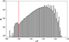 |
Fig. 1. Distribution of the LP parameter. The dashed red line marks our lower limit (LP = −50) that has been applied to exclude galaxies with poor SED fits, caused by unreliable photometric data. |
3.2. Lower redshift limit
To be consistent with Paper I, in this step of the selection we impose the same lower redshift limit of z = 0.02 on our sample, in addition to the upper limit of z = 0.213 already applied above. Our galaxy sample now consists of 82 981 total galaxies and 37 066 galaxies identified within 11 579 groups.
3.3. Hα star formation rate availability
Another small mismatch of 45 galaxies is found between our spectroscopic sample and the available SFR sample described in Section 2.2. Our final parent sample thus consists of a total of 82 936 galaxies and 37 040 galaxies belonging to the same groups. We summarise the complete selection process of the parent sample in Table 1. The final step of the selection process, namely, the application of the redshift-dependent stellar mass limit, is described in Section 5.2.
Our parent sample selection process.
4. Defining new subsamples
In this section, we describe how we determined two additional selections for our analysis. In particular, we describe how we distinguish between star-forming and passive galaxies (Sect. 4.1) as well as between centrals and satellites (Sect. 4.2).
4.1. Selecting star-forming/passive galaxies
In the literature, several approaches provide a separation between blue, star-forming, and red, passive galaxies, based on colour, SFR, morphology, or other galactic properties (Davies et al. 2019a). A common method, for instance, relies on specific colour cuts (Bell et al. 2003; Baldry et al. 2004; Peng et al. 2010).
However, at lower stellar masses, dust attenuation and complex SFHs make this distinction more problematic. To address this issue, Taylor et al. (2015) develop a statistical model that describes the observed galaxy distribution as the sum of two overlapping components, referred to as R-type and B-type, each defined by its own stellar mass function, colour-mass relation, and intrinsic scatter. They show that the previously observed differences between red and blue galaxy populations arise from inconsistent and arbitrary definitions, as hard cuts in CMDs lead to contamination and incompleteness, particularly at low masses where the two populations significantly overlap. While this method is flexible and highly effective, it is challenging to apply, as it consists of a complex 40-parameter probabilistic model tuned for nearby z < 0.12 galaxies.
Interestingly, Davies et al. (2019b) use a distinction based on an offset from the star-forming sequence (SFS). More precisely, they first consider a preliminary division at SFR/M = 10−10.5 yr−1; then, they perform two different least-squares regression fits to galaxies above and below this threshold (defining the star-forming and passive fits, respectively); finally, they identify the minimum density points along cross-sections perpendicular to the two fits, and the interpolation of those minima is taken as the final dividing line. The choice not to consider a separation at 1 dex below the SFS, as performed in other previous works, is due to the fact that within GAMA the SFS and the passive cloud show two different slopes. Therefore, this approach just provides a more robust division between the two populations.
Here, we implement the separation between SF and passive samples following a similar approach to that of Davies et al. (2019b). Since we do not want to be limited to their fixed, somewhat arbitrary initial division at SFR/M = 10−10.5 yr−1, we here implement an iterative procedure. At each iteration, the two regression fits and the dividing line are redetermined, using the current dividing line to define the star-forming and passive samples for the next step. The process continues until the dividing line converges, with a tolerance of 10−2. This slightly modified approach gives a final dividing line between the star-forming and passive populations which is independent of the choice of the initial division. In Fig. 2 we show the distribution of our parent sample in the log M − log SFR plane, split by star-forming (cyan dots) and passive (pink dots) galaxies. The star-forming and passive fits are marked as dashed blue and red lines, respectively, whereas the green solid line represents our final division. The density contours in Fig. 2 show that the dividing line accurately follows the minimum ridge. Our procedure yields a final separation that is very similar to the one obtained by Davies et al. (2019b).
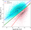 |
Fig. 2. Selection of star-forming and passive galaxies using the log M − log SFR plane. The dashed blue and red lines display the star-forming and passive population fits, respectively, whereas the solid green line displays our final dividing line. Star-forming galaxies are shown in cyan and passive galaxies in pink. Black dots refer to the 242 sources with LP < −50 (Sect. 3.1). |
We note that the black dots identify the 242 sources with LP < −50 (Sect. 3.1): this is to show that, since they are distributed approximately randomly in the log M − log SFR plane, their exclusion from our sample is expected not to introduce any bias. We also note that for 4165 galaxies our Hα-based SFR measurements provide only an upper limit. Among these, 128 have an upper limit that lies above our dividing line, and therefore their classification is uncertain. For these galaxies, we use the SED-based SFR measurements from PROSPECT instead. This results in 51 of these 128 galaxies being classified as star-forming. The remaining 77 galaxies are classified as passive. From our total parent sample of 82 936 objects, we thus identify 55 914 star-forming and 27 022 passive galaxies. Of these, 20 769 and 16 271 are grouped galaxies, respectively.
4.2. Grouped central and satellite galaxies
The G3C provides two different approaches for the determination of the central galaxy in a group. In particular, the catalogue identifies the source with the highest r-band luminosity (i.e. the brightest group galaxy, or BGG hereafter) and the source closest to the iterative centre of the group. This centre is defined through an iterative procedure where, at each iteration, the r-band centre of light is calculated and the most distant galaxy rejected until only two galaxies remain. Then, the brightest r-band galaxy is selected as central. See Sect. 4.2 of Robotham et al. (2011) for detailed explanations. Despite these two approaches producing similar results, Robotham et al. (2011) show that the iterative method always offers the most accurate agreement with the exact group centre. Therefore, as done by Vázquez-Mata et al. (2020), in this work we adopt this strategy to identify the central galaxy in each group.
From our final sample of 37 040 grouped galaxies, the iterative procedure identifies 11 038 centrals and 26 002 satellites. Here, we highlight that ∼97% of those centrals are also BGGs. Therefore, we do not expect our results to differ when selecting centrals according to the BGG approach.
5. Method
In this section, we describe the methods we used in our work: the modified maximum likelihood (MML) estimator for the construction of the GSMFs (Sect. 5.1) and the stellar mass completeness limit for the derivation of the selection function (Sect. 5.2).
5.1. Analytical parametrisation of the GSMFs
In this work, we adopted the well-established parametrisation that represents the GSMFs with either a single or a double Schechter function. The latter is given by:
 (3)
(3)
where  ,
,  and α1, α2 describe the normalisation and slope parameters, respectively, for the two components. The single Schechter function is simply obtained by neglecting the second term in parentheses.
Following the approach of Paper I, we fit the Schechter function using the MML estimation, which was comprehensively documented by Obreschkow et al. (2018). See Sect. 5.1 of Paper I for a detailed explanation of the MML approach.
Following the approach of Weigel et al. (2016), we do not impose any a priori assumption about whether the individual GSMFs are better described by a single or a double Schechter function. However, in all but one case, the decision between the two functional forms is straightforward and does not require a sophisticated model selection procedure. The only exception is the star-forming galaxy sample, for which we employ the statistical model selection techniques described in Sect. 7.1 to determine the preferred functional form.
5.2. Stellar mass completeness limit
As in Paper I, we followed the same approach presented by Pozzetti et al. (2010) for deriving the stellar mass limit, Mlim(z), above which our sample is complete at a given redshift. We refer to Sect. 5.2 of Paper I for a thorough explanation of this approach.
We once again emphasise that, after determining Mlim(z), the (small) remaining incompleteness of the selected subsample is not random, but rather depends on luminosity and stellar mass-to-light ratio (M/L), with faint, high-M/L galaxies being the most affected. For the purposes of this work, it would be inappropriate to adopt the selection function of the full sample as representative for the subsamples discussed in Section 4, since each of these exhibits its own Lr − M/Lr distribution, resulting in different levels of incompleteness. Unlike Paper I, we thus re-derive Mlim(z) individually for each subsample, that is, we adopt distinct selection functions for star-forming and passive galaxies (Sect. 4.1) as well as for centrals and satellites (Sect. 4.2). In practice, however, we find that using a single selection function (that of the full sample) produces essentially the same results. As in Paper I, we also impose a lower stellar mass limit of ![Mathematical equation: $ \log[M/(M_\odot\,h_{70}^{-1})] > 8.3 $](/articles/aa/full_html/2026/02/aa57424-25/aa57424-25-eq6.gif) to guarantee accurate GSMF measurements across all subsamples. Accordingly, we compute the GSMF of each subsample by providing the comoving distances, stellar masses and their uncertainties, selection function, and the chosen fitting function (i.e. double Schechter) using the MML framework.
to guarantee accurate GSMF measurements across all subsamples. Accordingly, we compute the GSMF of each subsample by providing the comoving distances, stellar masses and their uncertainties, selection function, and the chosen fitting function (i.e. double Schechter) using the MML framework.
6. Results
In this section, we present our results on the variation of the GSMF as a function of the subsamples defined in Sect. 4: star-forming and passive galaxies (Sect. 6.1), and centrals and satellites (Sect. 6.2). Furthermore, we study the dependence of the GSMF on group halo mass, Mhalo (Sect. 6.3).
6.1. How the GSMF differs in star-forming and passive galaxies
We went on to investigate the GSMF in star-forming and passive galaxies. As discussed in Sect. 4.1, we implemented a modified version of the method by Davies et al. (2019b) to separate the two populations in the log M − log SFR plane, using an iterative procedure that updates the linear regression fits and dividing line at each step until convergence. This approach removes any dependence on an arbitrary initial sSFR threshold.
In Fig. 3, we show the GSMFs for both our star-forming and passive galaxy populations, first using our full parent sample and then considering only galaxies inside and outside of groups (panels a, b, and c, respectively). In panel a, we also display the two Schechter components of each mass function as dashed lines. For the star-forming population, we note that the transition between the two components occurs at relatively high stellar masses compared to both the passive and global populations. In other words, in the mass range where the two Schechter components of the star-forming subsample intersect, both the passive and the total GSMFs are entirely dominated by the intermediate-mass component. As a result, the shape of the star-forming GSMF from low to intermediate masses is effectively governed by the low-mass component, while the intermediate-mass component primarily accounts for the exponential cut-off at the high-mass end. This behaviour makes the star-forming GSMF resemble a single Schechter function, which explains why previous works have typically found that a single component is a good description for such samples. Still, we find that the inclusion of a second component yields a slightly more accurate description, based on commonly used model selection criteria (see Sect. 7.1 for a more detailed discussion of this issue).
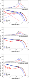 |
Fig. 3. GSMFs for our total, star-forming and passive galaxy populations, as indicated in the legend. Panel (a) full sample. Panels (b) and (c) grouped and ungrouped galaxies, respectively. In each sub-figure, the lower panel shows the GSMFs and the upper panel displays the raw number of galaxies as a function of stellar mass in each sample, as indicated. Dashed lines in panel (a) show the two individual Schechter components of each GSMF. |
In contrast, for the passive galaxy population, we confirm the need for a double Schechter function, as we clearly observe a low-mass upturn consistent with several previous findings (Peng et al. 2010; Baldry et al. 2012; Weigel et al. 2016), although some other studies do not report this upturn (e.g. Taylor et al. 2015; Moffett et al. 2016). This may be due in part to the method used to distinguish between star-forming and passive galaxies. The question thus arises whether the observed upturn may be due to an increased classification uncertainty towards the low-mass end. To investigate this, we visually inspected a random subsample of 20 galaxies with stellar masses below 109 M⊙, examining both their grz colour images and spectra. We find that ∼20% of the galaxies classified as passive in this mass range show clear signs of ongoing SF. Although this result demonstrates that some level of contamination of the passive subsample by star-forming galaxies is present, it is not sufficient to account for the pronounced low-mass upturn that we observe in the passive GSMF (see panel a of Fig. 3).
The best-fit double Schechter parameters are tabulated in Table 2 and shown in Fig. 4. Following the approach of Paper I, in these and similar tables and figures throughout this paper we only present our results regarding M★, α1, and α2, since we are more interested in any change of the shape of the mass function and less in its normalisation. As double Schechter fits can exhibit strong parameter degeneracies, we further examine the joint likelihood distributions of M★, α1 and α2. The 1σ, 2σ, and 3σ likelihood contours for the double Schechter parameters of all GSMFs presented in this paper are shown in Appendix A. Any claimed differences in the fitted parameters are based on these corner plots rather than on the best-fit values and their error bars alone.
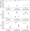 |
Fig. 4. Best-fit double Schechter function parameters of the GSMFs shown in Fig. 3, using the same colour-coding. The x-axes distinguish between all, grouped, and ungrouped galaxies; within each sample, the three ticks correspond to the total (T), star-forming (SF), and passive (P) subsamples. Corresponding corner plots illustrating the correlations among fitted parameters are provided in Figs. A.1–A.3. |
Best-fit double Schechter function parameters of the GSMFs of all, grouped, ungrouped, central, and satellite galaxies for different subsamples, as indicated.
We also test the robustness of our GSMF fits against variations in the dividing line used to separate star-forming and passive galaxies in Sect. 4.1, considering the 1σ confidence region around the fiducial slope and intercept. The resulting uncertainties in the double Schechter parameters are small (∼0.02 dex for log M★, 0.03 and 0.01 for α1 and α2, respectively), indicating that our conclusions are not significantly affected by these errors (see Appendix B for details).
When considering our full parent sample as well as grouped and ungrouped galaxies, we find that the total GSMF is dominated by passive and star-forming galaxies at the high- and low-mass end, respectively (cf. Fig. 3). Notably, the characteristic mass, M★, of the passive population almost coincides with that of the total sample in each case; in contrast, the low-mass slopes, α2, of the star-forming population are just slightly shallower compared to those of the total sample (cf. Fig. 4). We attribute these small discrepancies in M★ and α2 to the use of different selection functions for the passive and star-forming subsamples, compared to the total populations. On the other hand, the star-forming population exhibits systematically lower M★ values compared to the total sample, while the passive population shows steeper (i.e. lower) α2 values. Interestingly, the intermediate-mass slope, α1, of the total population is, in each case, steeper than those of the passive and star-forming components, and more closely resembles that of the passive population. These results confirm that star-forming and passive galaxies play a more prominent role in shaping the total GSMF at the low- and intermediate-to-high-mass regimes, respectively.
By comparing the grouped and ungrouped subsamples3, we find that both star-forming and passive galaxies outside of groups show systematically lower M★ values than their counterparts residing in groups, as already expected from the results in Paper I. This confirms that galaxies in groups are more likely to grow into more massive systems. In contrast, we observe that α1 for passive galaxies is shallower outside of groups, indicating a relatively higher abundance of intermediate-mass passive objects. Furthermore, the low-mass slope, α2, is slightly steeper for both star-forming and passive galaxies outside of groups, suggesting a relatively lower abundance of low-mass galaxies.
Finally, we note that uncertainties on α1 are relatively large for star-forming galaxies. This is because the two Schechter components intersect at relatively high masses, with the intermediate-mass component contributing significantly only at the high-mass end. As a result, its slope is poorly constrained. For passive galaxies, instead, the large errors on α2 are due to the limited number of low-mass objects available. These results still hold in Sect. 6.3, where we further investigate the dependence of the GSMF on Mhalo for both our star-forming and passive subsamples.
6.2. How the GSMF differs in central and satellites galaxies
Next we investigated the GSMF in central and satellite galaxies. As discussed in Sect. 4.2, centrals and satellites are identified using the iterative method from the G3C, which selects as central the brightest galaxy among the two closest to the group’s centre of light. Following Vázquez-Mata et al. (2020), ungrouped galaxies are excluded from the central galaxy population.
In Fig. 5 we show the GSMFs for our central, satellite, and ungrouped galaxy populations, first considering the entire samples and then their subdivision into star-forming and passive galaxies (left- and right-hand panels, respectively). Their best-fit double Schechter parameters are tabulated in Table 2 and shown in Fig. 6.
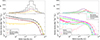 |
Fig. 5. GSMFs for our total, central, satellite, and ungrouped galaxy populations, as indicated in the legend. Left: GSMFs for each entire population. Right: Subdivision into star-forming and passive galaxies. In each sub-figure, the lower panel shows the GSMFs and the upper panel displays the raw number of galaxies as a function of stellar mass in each sample, as indicated. |
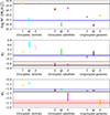 |
Fig. 6. Best-fit double Schechter function parameters of the GSMFs shown in Fig. 5, using the same colour-coding. The x-axes distinguish between central, satellite, and ungrouped galaxies; within each sample, the three ticks correspond to the total (T), star-forming (SF), and passive (P) subsamples. The black, blue and red horizontal bands show the results for the full parent, all-star-forming and all-passive samples, respectively, taken from Fig. 4. These reference lines are meant to be compared only with the T, SF, and P values in each subsample, respectively. Corresponding corner plots illustrating the correlations among fitted parameters are provided in Figs. A.4 and A.5. |
When considering the entire samples, we find that the total GSMF is dominated by centrals and ungrouped galaxies at the high- and low-mass ends, respectively (cf. Fig. 5, left-hand panel). Notably, the characteristic mass, M★, of central galaxies closely matches that of the total sample, with satellites and ungrouped galaxies showing progressively lower values. Small differences in the fitted parameters across different samples may arise from the use of different selection functions, but these do not affect the main trends discussed below. In contrast, the low-mass slope, α2, of ungrouped galaxies is very similar to that of the total sample, while satellites and centrals exhibit increasingly shallower slopes. This results in a decreasing trend for both M★ and α2 from centrals to ungrouped galaxies (cf. Fig. 6). Interestingly, the intermediate-mass slope, α1, of satellites is in striking agreement with that of the total population, whereas both centrals and ungrouped galaxies show significantly higher (i.e. shallower) values. This may suggest that satellites play the dominant role in shaping the total GSMF in this stellar mass regime.
When splitting into star-forming and passive galaxies, we observe consistent trends across all populations. In each case, passive galaxies exhibit higher M★ values and steeper α2 slopes compared to their star-forming counterparts (cf. Fig. 5, right-hand panel). The only exception is the α2 values for central galaxies, since the passive subpopulation is best fit by a single Schechter function, for which only α1 is defined. Specifically, we observe a decreasing trend for M★ from centrals to satellites to ungrouped galaxies, within both the star-forming and passive subpopulations. Notably, the M★ value of the central star-forming population is comparable to that of the all-star-forming sample, and the same holds for the passive central population with respect to the all-passive sample (cf. Table 2).
This finding demonstrates that central star-forming and passive galaxies dominate the high-mass end of the corresponding total GSMFs. A similar trend is observed for α2 within the star-forming subpopulation, with increasingly steeper slopes from centrals to satellites to ungrouped galaxies. For the passive subpopulation, although α2 is not available for centrals, the slope still steepens from satellites to ungrouped galaxies. In particular, the α2 value of the all-star-forming galaxy sample lies between those of the satellite and ungrouped populations, showing good agreement with both. In contrast, the all-passive galaxy sample exhibits a value of α2 that is in striking agreement with that of the ungrouped passive population. These findings suggest that both satellite and ungrouped galaxies shape the low-mass end of the star-forming GSMF, whereas the passive GSMF in this regime is primarily shaped by ungrouped galaxies. For α1, the trend remains consistent with the previous results only within the star-forming subpopulation, with increasingly steeper values from centrals to satellites to ungrouped galaxies. In particular, the α1 value of the all-star-forming galaxy sample is comparable to those of the satellites and ungrouped star-forming populations. For passive galaxies, the value of α1 is closest to that of passive satellites, with centrals and ungrouped galaxies showing significantly higher values (i.e. shallower) values. These findings suggest that both satellite and ungrouped galaxies shape the intermediate-mass regime of the star-forming GSMF, whereas the passive GSMF in this regime is predominantly shaped by satellite galaxies alone.
By comparing the grouped (both central and satellite) and ungrouped subsamples, we confirm the trends found in Sect. 6.1 regarding M★ and α2. Isolated galaxies exhibit lower M★ and steeper α2 values compared to galaxies in groups.
6.3. GSMF dependence on group halo mass
To study the dependence of the GSMF on group halo mass, Mhalo, we are forced to discard 1055/11 579 (9.1%) of our groups for which the G3C does not report any Mdyn values because the measured velocity dispersion of these groups is smaller than its error. These are overwhelmingly groups with multiplicity NFOF = 2. Our total sample now consists of 10 524 groups containing 34 931 galaxies.
We now bin galaxies according to the mass of the group that they belong to into four different bins in ![Mathematical equation: $ \log [M_{\mathrm{halo}}/(M_{\odot}\,h^{-1}_{70})] $](/articles/aa/full_html/2026/02/aa57424-25/aa57424-25-eq12.gif) : ≤12.65, 12.65 − 13.3, 13.3 − 13.85, and > 13.85. This choice is made to maintain approximately the same number of galaxies per bin. Our resulting GSMFs, colour-coded by Mhalo, are shown in Fig. 7. Panel a shows the GSMFs as a function of Mdyn, while panels b and c further distinguish between passive and star-forming galaxies, and between central and satellite galaxies, respectively. Their best-fit double Schechter parameters are tabulated in Table 3 and shown in Fig. 8.
: ≤12.65, 12.65 − 13.3, 13.3 − 13.85, and > 13.85. This choice is made to maintain approximately the same number of galaxies per bin. Our resulting GSMFs, colour-coded by Mhalo, are shown in Fig. 7. Panel a shows the GSMFs as a function of Mdyn, while panels b and c further distinguish between passive and star-forming galaxies, and between central and satellite galaxies, respectively. Their best-fit double Schechter parameters are tabulated in Table 3 and shown in Fig. 8.
Best-fit double Schechter function parameters of the GSMFs of grouped galaxies for different subsamples, as indicated.
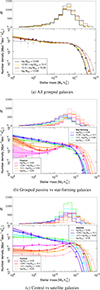 |
Fig. 7. GSMFs of our grouped galaxy subsample colour-coded by Mhalo, as indicated in the legend. Panel a GSMFs as a function of Mdyn. Panels b and c further distinguish between passive and star-forming galaxies, and between central and satellite galaxies, respectively. In each sub-figure, the lower panel shows the GSMFs and the upper panel displays the raw number of galaxies as a function of stellar mass in each sample, as indicated. |
When we consider our entire grouped galaxy sample, we note that the characteristic mass, M★, increases systematically with Mdyn, indicating that more massive halos tend to host more massive galaxies. Both the intermediate-mass slope, α1, and the low-mass slope, α2, exhibit a similar trend, namely a mild steepening when moving from low- to intermediate-mass halos, followed by a progressive shallowing as Mdyn continues to increase. We note that the exceptionally high value of α1 in the most massive halo bin reflects that the GSMF can be more accurately described by a single Schechter function, as the intermediate-mass component has negligible influence on the overall shape. Unsurprisingly, our findings are essentially identical with the main results of Paper I, where we investigated the dependence of the GSMF on Mhalo using four different halo mass estimators, despite the use of a different photometry and revised stellar mass estimates in the present analysis.
When we further distinguish between passive and star-forming galaxies, we observe distinct behaviours in the evolution of M★. Passive galaxies follow a consistent trend similar to the overall sample, with M★ increasing steadily as Mdyn grows. Star-forming galaxies show a similar trend, except for the highest halo mass bin where M★ actually decreases. This decline may reflect environmental effects suppressing SF in the most massive halos. However, passive galaxies show consistently higher M★ values than star-forming galaxies, confirming their tendency to be more massive at fixed halo mass. Regarding α2, both populations exhibit a consistent trend similar to the overall sample, namely a steepening from low to intermediate halo masses, followed by a shallowing as Mdyn continues to increase. However, this trend is more pronounced in passive galaxies, which show a stronger steepening and subsequent flattening. In contrast, star-forming galaxies display a milder but more extended steepening, with the shallowing occurring only at the highest halo mass bin. Similarly, α1 shows a comparable evolution for both star-forming and passive galaxies. In both cases, there is a steepening with increasing Mdyn, followed by a shallowing at the most massive halos. As previously noted for the entire grouped galaxy sample, the exceptionally high values of α1 in the highest halo mass bin likely indicate that the intermediate-mass component contributes negligibly to the shape of the GSMF. Consequently, those mass functions are better represented by a single Schechter function, with the intermediate-mass slope effectively losing its physical meaning.
When we separate galaxies into centrals and satellites, M★ still increases steadily with Mdyn, regardless of the population, indicating that more massive halos host more massive galaxies. However, central galaxies show consistently higher values than satellites, confirming their tendency to be more massive at fixed halo mass. Regarding α2, central galaxies exhibit a mild but progressive steepening as Mdyn increases. This indicates that the relative abundance of low-mass centrals gradually grows in more massive halos. In contrast, satellite galaxies show the opposite behaviour, namely α2 becomes progressively shallower with increasing Mdyn, indicating a relative decrease in the number of low-mass satellites in more massive halos. Concerning α1, central galaxies follow a trend similar to that observed in the overall sample, with a steepening from low to intermediate halo masses, followed by a progressive shallowing as Mdyn continues to increase. In contrast, satellites exhibit the opposite trend, with α1 becoming shallower as Mdyn increases and then steepening in the highest halo mass bin. These distinct behaviours for central and satellite galaxies presumably reflect different quenching mechanisms shaping these galaxy populations.
7. Discussion
In this section, we discuss and compare our results on the variation of the GSMF for star-forming and passive galaxies (Sect. 7.1), for centrals and satellites (Sect. 7.2), and as a function of group halo mass (Sect. 7.3), in the context of other similar studies.
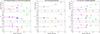 |
Fig. 8. Best-fit double Schechter function parameters of the GSMFs shown in Fig. 7, using the same colour-coding by Mhalo. Panel a is in the centre, while panels b and c are on the left and right, respectively. For clarity, the vertical error bars corresponding to the passive galaxies in the left-hand panel and the centrals in the right-hand panel have been slightly offset to the right. Corresponding corner plots illustrating the correlations among fitted parameters are provided in Figs. A.6–A.8. |
7.1. How the GSMF differs in star-forming and passive galaxies
Peng et al. (2010) presented an empirical model describing galaxy evolution based on observations from the SDSS and zCOSMOS, emphasising the roles of mass and environment. The study demonstrates that the effects of mass and environment on galaxy quenching are fully separable up to redshift z ∼ 1. This suggests distinct mechanisms are at play, where mass quenching is related to a galaxy’s SFR, and environment quenching is linked to the growth of large-scale cosmic structures. The combination of these two quenching processes, plus some additional quenching due to merging, naturally produces (1) a quasi-static single Schechter mass function for star-forming galaxies with an exponential cut-off at a value M★ that is set uniquely by the constant of proportionality between the SF and mass quenching rates, and (2) a double Schechter function for passive galaxies. Remarkably, the characteristic mass of the star forming population remains constant up to redshift z ∼ 2, indicating a universal efficiency of mass quenching over cosmic time. For the passive population, the dominant component (at high masses) is produced by mass quenching and shares the same M★ as star-forming galaxies but has a low-mass slope, α1,P, differing by approximately α1,P − αSF ≈ 1. The other component is produced by environmental effects and has the same M★ and α2,P as star-forming galaxies, but lower amplitude depending on the environment, with high-density environments showing a stronger component.
Several key predictions of the empirical model proposed by Peng et al. (2010) are not supported by our results. The only qualitative agreement that we observe is in the functional form of the GSMFs. Specifically, we confirm that both the total and the passive populations are best described by a double Schechter function fit, whereas the star-forming population is well approximated by a single Schechter function. Although we show that a double Schechter fit provides a marginally better representation, the transition between the two components occurs at very high stellar masses. As a consequence, the star-forming GSMF is dominated by its low-mass component across most of its mass range, and its overall shape closely resembles a single Schechter function, consistent with Peng et al. (2010). Nonetheless, our analysis shows that adding a second component produces a slight improvement in the fit, possibly reflecting early signs of quenching at the intermediate-mass regime of the star-forming population. However, except for this structural similarity, our results diverge significantly from the predictions of Peng et al. (2010).
Comparisons between the best-fit double Schechter function parameters from Peng et al. (2010) and our results are shown in Table 4 and Fig. 9. To investigate the role of environment in shaping the GSMF, we also compare our measurements for grouped and ungrouped galaxies with the high- and low-density bins (D4 and D1, respectively) presented by Peng et al. (2010). While our environmental classification is based on group membership within the GAMA survey, Peng et al. (2010) use local overdensity quartiles derived from the zCOSMOS sample, where density is estimated via the fifth nearest neighbour method.
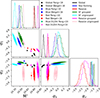 |
Fig. 9. Comparison between our best-fit double Schechter function parameters and literature values for different subsamples, as indicated in the legend. The likelihood contours show the 1σ, 2σ, and 3σ confidence regions for our fits. For each distribution, 104 random samples were generated. Symbols indicate the best-fit values from previous studies: circles for Peng et al. (2010) and squares for Weigel et al. (2016). |
First, contrary to their model’s prediction that the characteristic stellar mass, M★, should be the same for star-forming and passive galaxies, regardless of environment, we find much larger discrepancies between the two populations. Whereas Peng et al. (2010) report a difference of ΔM★ ≈ 0.05 dex between their full star-forming and passive samples, and a maximum offset of ΔM★ ≈ 0.16 dex when comparing their star-forming D1 and passive D4 bins, our results show significantly larger variations, with ΔM★ ≈ 0.35 dex for our full samples and up to ΔM★ ≈ 0.54 dex between our grouped and ungrouped subsamples. Similarly, the low-mass slope, α2, which in Peng et al. (2010) is nearly identical for star-forming and passive galaxies, both for the full samples and across different environments, differs substantially in our results. The empirical framework proposed by Peng et al. (2010) assumes that mass and environment quenching act independently, and that the characteristic mass, M★, remains constant because the mass-quenching rate scales directly with the SFR. The strong dependences of both M★ and α2 on environment revealed here suggest that these assumptions break down: environmental conditions seem to modulate the efficiency of mass quenching, indicating that the two processes are physically coupled rather than independent. Similarly, the differences in M★ between star-forming and passive populations also imply that mass quenching cannot be simply proportional to SFR, and that additional factors, such as structural properties or local density, likely influence the quenching process.
Regardless of our environmental classification (i.e. full sample, grouped, or ungrouped galaxies), we find that the α2 value for passive galaxies is significantly steeper than those of star-forming and total populations, which instead display relatively similar values. In the Peng et al. (2010) model, environment quenching is expected to be a mass-independent process that only changes the normalisation of the passive GSMF. The fact that we observe systematically steeper slopes for passive galaxies in denser environments once again indicates that environmental quenching may depend on stellar mass, modifying the shape of the mass function itself.
Interestingly, one prediction from Peng et al. (2010) that still holds in our results is the relation α1,P − αSF ≈ 1, which we confirm for both our full sample (=0.96) and our grouped galaxy population (=0.82). However, this trend does not extend to ungrouped galaxies, for which α1,P − αSF = 1.42, suggesting that the connection between star-forming and passive slopes may be more sensitive to the environment than previously thought.
Together, the persistence of α1,P − αSF ≈ 1 and the agreement in the overall shapes of the GSMFs indicate that the empirical framework proposed by Peng et al. (2010) still provides a good phenomenological description of galaxy populations. However, the deviations in M★ and the environmental trends discussed above suggest a more intricate interplay between mass and environment quenching than assumed in their model.
We caution here that our classification of galaxies into star-forming and passive populations is based on direct measurements of SF activity via Hα emission, while Peng et al. (2010) use broad-band photometric colours. These choices may partly account for the discrepancies that we observe in our results.
Finally, we have tested whether the differences in the M★ values between star-forming and passive galaxies could be driven by our choice of the fitting function (i.e. using a double instead of a single Schechter parametrisation). When fitting the star-forming population with a single Schechter function, as done by Peng et al. (2010), the inferred M★ shifts to higher values, partially reducing the discrepancies with the passive population. Specifically, M★ increases from 1010.48 to 1010.74 M⊙ for the full sample, from 1010.52 to 1010.80 M⊙ for the grouped subsample, and from 1010.38 to 1010.68 M⊙ for the ungrouped subsample. Although a significant mismatch with the M★ value of the passive population persists in all cases, a large part of the star-forming/passive M★ discrepancy rests on our choice of representing the star-forming population with a double Schechter function. Hence, the question arises as to how robust this choice is when faced with variations among our star-forming versus passive classification method.
In Sect. 6.1 we already investigated the sensitivity of the fitted double Schechter function parameters to variations of our dividing line used to separate star-forming and passive galaxies. We now also test the robustness of the model selection in favour of the double Schechter function. For each of the 100 pairs extracted from the 1σ confidence region of our fiducial dividing line in the log M − log SFR plane, we perform the GSMF fit using both a single and a double Schechter function, and compute different model selection statistics such as the log-likelihood ratio test (LRT), the Bayesian information criterion (BIC; Schwarz 1978), the Akaike information criterion (AIC; Akaike 1974), and the Bayesian evidence4.
The LRT values, as well as the differences in BIC and AIC between the single and double Schechter models, are consistently very high. According to the scale proposed by Jeffreys (1939), such values provide decisive evidence in support of the more complex model (i.e. double Schechter). Likewise, the strongly negative differences in Bayesian evidence further confirm that the double Schechter representation is robust to small changes in the classification process. In particular, we explore the distribution of the LRT statistic derived from the 100 different star-forming subsamples, and shown in Fig. 10. Our observed LRT value, shown as a dashed red line, lies near the peak of the simulated distribution, which exhibits no significant tails towards lower or higher values. This finding indicates that, regardless of how the dividing line is perturbed within the 1σ region, the double Schechter model reliably provides a significantly better fit to the data. Therefore, our preference for a double Schechter function is well justified and not an artefact of how we select star-forming and passive galaxies. We thus conclude that the discrepancies that we observe with the results of Peng et al. (2010) cannot be attributed to the functional form alone, but rather arise from real deviations in the assumptions of their model.
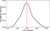 |
Fig. 10. Distribution of the LRT statistic obtained from 100 star-forming subsamples. The red dashed line marks our observed LRT value, which lies near the peak of the simulated distribution. This compatibility suggests that the data are consistent with the double Schechter model representing the true distribution, whereas the single Schechter function fails to provide an accurate description. |
Taylor et al. (2015) investigate the GSMFs for their blue/star-forming (B-type) and red/passive (R-type) populations, based on a sample of M★ > 108.7 M⊙ and z < 0.12 galaxies from the GAMA survey. When modelling the GSMFs, they use a double Schechter function for both subsamples. For the B-type population, the secondary component detects a small deficit of galaxies observed in the range 1010 − 1010.3 M⊙, which corresponds to the apparent upturn observed in the overall GSMF. This results in a slightly more complex shape that cannot be fully described by a single Schechter function. For the R-type population, in contrast, the secondary component becomes negligible above 109.5 M⊙, failing to reproduce the apparent low-mass upturn in the red GSMF observed by Peng et al. (2010). This discrepancy is mainly due to broader selection criteria for the red population, which includes a significant number of star-forming galaxies with young stellar populations. Such misclassifications are particularly common at low masses, where red galaxies are intrinsically rare, and a simple colour cut would classify the reddest tail of the blue population as red galaxies. It is important to note, however, that Taylor et al. (2015) do detect a similar low-mass upturn in their R-type GSMF. This upturn is more pronounced when the B/R classification is based on the intrinsic, rather than the restframe, CMD. However, they do not consider this feature to be robust.
We also confirm that the double Schechter function provides a better representation of both blue/star-forming and red/passive galaxies. However, we do not find strong evidence that the apparent upturn in the overall GSMF is primarily driven by the blue population. In contrast to Taylor et al. (2015), we clearly observe a low-mass upturn in the red population, which is more evident for ungrouped than grouped galaxies, but still present when considering the full passive sample (cf. Fig. 3). Although we confirm that the low-mass Schechter component of the red GSMF becomes negligible above M★ ≈ 109.5 M⊙, the upturn we observe may also be due to the fact that our sample extends down to M★ ≈ 108.3 M⊙, somewhat deeper than the limit of 108.7 M⊙ adopted by Taylor et al. (2015). While the R-type GSMF remains relatively flat below 1010.5 M⊙ and is systematically lower at low masses compared to the red GSMFs available in the literature, we find excellent agreement at the very low-mass end in terms of number density between our all-passive GSMF and the R-type GSMF of Taylor et al. (2015). This consistency is particularly evident when the B/R classification is based on the intrinsic, rather than the restframe, CMD. The smooth decline of the R-type fraction toward lower stellar masses observed by Taylor et al. (2015) indicates that, while more massive galaxies are more likely to host older stellar populations, quenching cannot be attributed to stellar mass alone.
Weigel et al. (2016) present a comprehensive study of the GSMF at 0.02 ≤ z ≤ 0.06, using data from the SDSS DR7. Their analysis investigates how the GSMF depends on various galaxy properties and environmental parameters. To this end, the main sample is divided into more than 130 subsamples based on morphology, colour, sSFR, central versus satellite classification, halo mass, and local density. For each subsample, they independently evaluate both single and double Schechter fits and use a likelihood ratio test to identify the model that best describes the data. The classification of blue and red galaxies does not follow the method of Taylor et al. (2015), but rather relies on two linear cuts in the CMD, which identify blue, red, and intermediate green galaxies lying between the two cuts. Blue galaxies are generally well described by a single Schechter function with a relatively steep low-mass slope, whereas red galaxies show an upturn at the low-mass end, which requires a double Schechter fit. Weigel et al. (2016) find their blue and red GSMFs to be systematically lower than those presented by Peng et al. (2010), likely because they explicitly identify a green valley population, which reduces the number densities of both blue and red galaxies. Nevertheless, their GSMFs are more consistent with those of Taylor et al. (2015) and with our own, despite their use of a single Schechter function.
Direct comparisons of the best-fit double Schechter parameters (Table 4 and Fig. 9) show that the total and red GSMFs presented by Weigel et al. (2016) are remarkably consistent with our mass functions, and significantly closer than those reported by Peng et al. (2010). In particular, the values of M★ for both the total and red populations differ by ≈0.05 dex, whereas the slopes α1 and α2 are consistent within the uncertainties. This agreement is particularly notable given the differences in methodology and classification criteria. For the blue population, however, the discrepancy is more pronounced. Weigel et al. (2016) find a higher M★ and a significantly shallower α2. This difference is attributed to our use of a double Schechter function, which provides a better fit to the mass function, particularly around the intermediate-mass regime, and likely results in a lower M★ and a steeper α2.
Best-fit double Schechter function parameters of the GSMFs of star-forming and passive galaxies, corresponding to blue and red populations in other studies, as indicated.
7.2. How the GSMF differs in central and satellite galaxies
In a follow-up study, Peng et al. (2012) investigate the environmental effects on galaxy evolution, focusing on the quenching of satellite galaxies within SDSS groups. They find that the environmental quenching effects identified in Peng et al. (2010) can be entirely attributed to the satellites, while central galaxies (including isolated singletons) are affected only by internal, mass-dependent processes. For centrals, the red fraction depends solely on stellar mass and shows no dependence on environmental factors such as local overdensity or halo mass. In contrast, the red fraction of satellites increases with both stellar mass and local overdensity, but interestingly not with global group properties, such as richness or the parent DM halo mass. Moreover, the fraction of blue central galaxies that are quenched when they become satellites (the so-called satellite quenching efficiency) is found to be largely independent of stellar mass but strongly dependent on local overdensity (which reflects a galaxy’s position within the group) rather than the overall DM halo mass. The phenomenological model adopted in Peng et al. (2010) also predicts the GSMFs of star forming and passive centrals and satellites. In particular, the star forming population, whether it consists of centrals or satellites, follow a single Schechter function with the same M★, which is independent of halo mass (above 1012 M⊙). This confirms the universality of the mass-quenching process, which operates through the same physical mechanism for both types of galaxies, unaffected by their environment. For the passive population, centrals are well described by a single Schechter, whereas satellites require a double Schechter function, with one component attributed to mass quenching and the other to satellite quenching.
If we adopt a similar classification, namely, defining as centrals both central galaxies in groups and isolated singletons, we find that our results are broadly consistent with this framework. In terms of functional form, we show that the GSMF of the passive central population is well described by a single Schechter function, in line with the results of Peng et al. (2012), who associate this shape with only mass quenching. Similarly, the GSMFs of the star-forming population, whether centrals or satellites, can also be reasonably fitted with a single Schechter function. Although a double Schechter may offer a slightly more accurate fit, the α1 values being very close to zero suggest that the intermediate-mass component does not play a significant role. Therefore, the only subsample that clearly requires a double Schechter function fit is the passive satellite population, as also shown by Peng et al. (2012), where the excess at low masses is attributed to environment (satellite) quenching.
In Table 5 and Fig. 11, we also provide comparisons of the best-fit double Schechter function parameters from Peng et al. (2012) with our results. Although the values differ, possibly due to differences in photometry, stellar mass estimation methods, and GSMF measurement techniques, the observed trends are in good qualitative agreement. The characteristic stellar mass, M★, systematically increases from satellite to central galaxies, and from blue to red populations. In both studies, red centrals exhibit the highest values, followed by red satellites, blue centrals, and blue satellites. We find a difference in M★ of 0.10 dex between centrals and satellites, for both red and blue populations, compared to 0.09 dex and 0.02 dex, respectively, as reported by Peng et al. (2012). For the low-mass slopes, α2, of the blue populations, we find similar values for blue centrals and satellites. In contrast, Peng et al. (2012) show a shallower and a steeper α2 for blue centrals and satellites, respectively, indicating a stronger environmental dependence in the low-mass regime. This discrepancy might be attributed to the different fitting procedures: while we adopt a double Schechter function, Peng et al. (2012) use a single Schechter, which potentially influences the derived low-mass slope values. Interestingly, our intermediate-mass slope, α1, for red central galaxies is fully consistent with the value shown by Peng et al. (2012), within the uncertainties, confirming that a single Schechter function adequately describes this subsample. Finally, for the red satellite galaxies, we find that our values of α1 and α2 are significantly steeper than those reported by Peng et al. (2012). This indicates a more pronounced decline in the GSMF at both intermediate and low masses in our red satellite population. Nevertheless, we confirm that a double Schechter function remains the most appropriate fit, consistent with Peng et al. (2012).
Best-fit double Schechter function parameters of the GSMFs of central and satellite galaxies for different works, as indicated.
In their study, Weigel et al. (2016) also find that the total GSMFs of both central and satellite galaxies are better described by a double Schechter function. For centrals, this is due to an excess of high-mass galaxies, which requires an additional high-mass component. Satellites, on the other hand, show a pronounced upturn at the low-mass end, which also requires an additional steeper component. This result is in contrast with Yang et al. (2009), who suggest that the satellite GSMF can be sufficiently fit by a single Schechter function.
Direct comparisons of the best-fit double Schechter parameters for central and satellite galaxies (Table 5 and Fig. 11) show overall good agreement between our results and those of Weigel et al. (2016). The characteristic mass, M★, differs by less than 0.05 dex in each subsample. Similarly, α1 for satellites and α2 for centrals are consistent within the uncertainties. However, we find a notably higher (i.e. less negative) value of α1 for central galaxies, indicating a flatter slope at intermediate masses. For satellites, instead, our α2 is significantly shallower than in Weigel et al. (2016), suggesting a less pronounced upturn at the low-mass end. These differences may be attributed to the different sample selection and group identification method. Nonetheless, the overall agreement in M★ and the general shape of the GSMFs confirm the consistency of the main trends across both studies.
When splitting both centrals and satellites into blue and red galaxies, Weigel et al. (2016) model all GSMFs using a single Schechter function. This approach is consistent with our results and those of Peng et al. (2012) for centrals and blue satellites, but not red satellites, for which a double Schechter is needed to capture the low-mass upturn. These differences may be attributed to their use of two colour cuts to explicitly define three separate populations (blue, green, and red) rather than just a binary classification. As a result, a significant fraction of objects falls into the green valley, reducing the number densities of both the blue and red samples. This also makes their results not directly comparable to our work or that of Peng et al. (2012), where no green population is explicitly defined. We note that Weigel et al. (2016) adopt a double Schechter function for both green centrals and green satellites. This suggests that the steep low-mass component that we observe in the red satellite subpopulation may instead be captured by their green subsample, making direct comparisons more challenging.
A complementary analysis by Davies et al. (2019b), based on the G3C, investigates the passive fractions of central and satellite galaxies as a function of both stellar and halo mass. By taking the appropriate ratios of the GSMFs presented in Sect. 6.2, we are able to reproduce all of their results. Specifically, we confirm that the passive fractions of both centrals and satellites increase with halo mass when considering all stellar masses, and also increase with stellar mass when considering all halo masses. Moreover, satellites exhibit higher passive fractions than centrals at fixed stellar mass for ![Mathematical equation: $ \log[M/(M_{\odot}\,h^{-2}_{70})] < 11 $](/articles/aa/full_html/2026/02/aa57424-25/aa57424-25-eq40.gif) , consistent with the environmental quenching scenario for low-mass satellites. Even when controlling for both stellar and halo mass, we find that satellite galaxies have systematically higher passive fractions than centrals, particularly at low stellar masses and in high-mass halos. These results are expected, as we adopt a similar method for separating star-forming and passive galaxies (see Sect. 4.1). This consistency confirms the robustness of our classification and supports the reliability of our derived GSMFs and their environmental trends.
, consistent with the environmental quenching scenario for low-mass satellites. Even when controlling for both stellar and halo mass, we find that satellite galaxies have systematically higher passive fractions than centrals, particularly at low stellar masses and in high-mass halos. These results are expected, as we adopt a similar method for separating star-forming and passive galaxies (see Sect. 4.1). This consistency confirms the robustness of our classification and supports the reliability of our derived GSMFs and their environmental trends.
7.3. GSMF dependence on group halo mass
Weigel et al. (2016) also investigate how the GSMF varies as a function of halo mass, Mhalo. Although their analysis is based on only three bins, the identified trends are fully consistent with ours. In particular, they report a systematic increase of the characteristic mass, M★, with Mhalo and, for the low-mass slope, α2, a steepening from low to intermediate halo masses, followed by a shallower slope in the most massive halos. Moreover, they find that a single Schechter function better describes the GSMF in the highest halo mass bin. This confirms the behaviour we also observe, where the intermediate-mass component becomes negligible and the double Schechter fit effectively reduces to a single component. These trends for M★ and α2 with Mhalo are preserved when Weigel et al. (2016) split their sample into red and blue galaxies, although their classification explicitly identifies a green valley population in between. Specifically, they find a systematic increase in M★ as Mhalo increases for both red and blue galaxies, with red galaxies still showing higher M★ values than their blue counterparts at fixed halo mass. Similarly, α2 shows a steepening from low to intermediate halo masses, followed by a shallower value in the most massive halos. These trends are in excellent agreement with our findings when we divide galaxies into passive and star-forming populations. Despite differences in data sets, sample selection, classification methods, and halo mass bins, our results on M★ and α2 seem to be generally comparable with those of Weigel et al. (2016) across corresponding halo mass regimes.
In another study, Vázquez-Mata et al. (2020) investigated how the GSMFs of central and satellite galaxies depend on the host DM halo mass, using data from the GAMA survey. Central GSMFs are well described by log-normal functions, especially at high masses, for both blue and red populations. However, at low halo masses, they observe a slight excess of low-mass centrals, indicating that the log-normal function underestimates their abundance in this regime. In contrast, satellite GSMFs are generally well described by single Schechter functions. Nonetheless, at high halo masses, a slight excess of high-mass satellites is observed. Central galaxies show a clear increase in their characteristic stellar mass, M★, with halo mass. At fixed halo mass, red centrals are systematically ≈0.2 dex more massive than blue centrals. Similarly, satellite galaxies exhibit an increase in their characteristic stellar mass as halo mass grows. This reflects the mass–richness correlation in galaxy groups, where more massive halos host both more numerous and more massive satellites. While the general trends are consistent with previous studies, Vázquez-Mata et al. (2020) find a stronger dependence of the characteristic stellar mass of both centrals and satellites on halo mass compared to Yang et al. (2009), likely due to differences in group definitions and halo mass estimates. In addition, they do not confirm the systematic steepening of the satellite GSMF low-mass slope with halo mass reported by Yang et al. (2009), in either blue or red populations. Instead, they find the steepest slopes in the lowest mass halos, suggesting that faint, low-mass satellite galaxies are relatively more abundant in low-mass environments. Finally, they show that the fraction of red galaxies increases with halo mass. Further evidence for environmental quenching comes from the observed increment in the red-to-blue galaxy ratio within groups since z ∼ 0.3, compared to the field. This suggests that group environments continuously quench SF in infalling galaxies.
Although Vázquez-Mata et al. (2020) model central and satellite GSMFs using different functional forms than those adopted in this work, a meaningful comparison with our results is still possible. First, we confirm the increase of M★ with Mhalo for both central and satellite galaxies. Specifically, our M★ values for satellites in all halo mass bins agree well with those reported by Vázquez-Mata et al. (2020), despite differences in binning and data sets. For centrals, their M★ values tend to be slightly higher than ours, especially in the most massive halos. Nevertheless, both studies consistently find that, at fixed halo mass, central galaxies are more massive than satellites. Regarding the low-mass end slope, both analyses report a general shallowing of the GSMF with increasing halo mass. As presented in Vázquez-Mata et al. (2020), this trend is not strictly monotonic, as the slope slightly steepens in their highest halo mass bin, but the overall behaviour is still comparable. On the other hand, our α values are systematically steeper across all bins, which may be attributed to our use of a double Schechter function, as well as to differences in binning and data sets.
8. Conclusions
We employed the equatorial GAMA II dataset at z ≤ 0.213 to construct multiple GSMFs. For our analysis, we made use of various GAMA data products: stellar masses (Sect. 2.1; Robotham et al. 2020), Hα-derived SFRs (Sect. 2.2; Davies et al. 2016), and the G3C (Sect. 2.3) for the identification of groups (Robotham et al. 2011). Our magnitude-limited parent galaxy sample (the selection of which is summarised in Table 1) consists of 82 936 galaxies and 11 579 groups. To account for completeness, we re-derived the redshift-dependent stellar mass limit for each subsample considered. This differs from Paper I, where a single selection function was applied. However, adopting a global selection function yields nearly identical results.
We investigated how the low-redshift GSMF varies across different galaxy populations (star-forming versus passive in Sect. 6.1, and centrals versus satellites in Sect. 6.2) and as a function of halo mass (Sect. 6.3). We noted first that the GSMFs of star-forming and passive galaxies show distinct shapes: passive galaxies require a double Schechter function to capture the low-mass bump, while the star-forming population appears well approximated by a single Schechter function due to its high-mass cut-off being dominated by the intermediate-mass component. Nonetheless, we find that a double Schechter provides a slightly more accurate description for the star-forming sample. Our results confirm that the total GSMF is dominated by star-forming galaxies at the low-mass end and by passive galaxies in the intermediate-to-high-mass regime (cf. Fig. 3). We also tested the robustness of our star-forming and passive GSMFs against small variations of the star-forming versus passive classification by varying the dividing line in the log M − log SFR plane within its 1σ confidence region. The resulting uncertainties in the double Schechter function parameters were similar or smaller to the random errors, confirming that our results are robust against small perturbations in the classification. Comparing galaxies inside and outside of groups, we found that galaxies in groups have higher M★ and shallower α2 for both our star-forming and passive populations, indicating, respectively, that more massive systems preferentially form in groups and that groups host a relatively lower abundance of low-mass galaxies.
Next, we examined the GSMFs of central and satellite galaxies. We found that central and ungrouped galaxies dominate the high- and low-mass end of the total GSMF, respectively (cf. Fig. 5). M★ shows a decreasing trend from centrals to satellites to ungrouped galaxies, consistently across the full, star-forming, and passive samples. A similar trend is observed for α2, with steeper values for isolated systems, although for passive centrals the fit requires only a single Schechter component (cf. Fig. 6). Interestingly, the α1 values of satellites closely match results characterising the total population, suggesting that satellites play a key role in shaping the intermediate-mass regime of the total GSMF. When separating by SF activity, we find that central star-forming and passive galaxies dominate the high-mass ends of their respective GSMFs. In contrast, the low-mass end of the star-forming GSMF is shaped by both satellite and ungrouped galaxies, while that of the passive GSMF is primarily shaped by ungrouped galaxies. These trends confirm and extend the environmental dependencies observed in Sect. 6.1: galaxies in groups show higher M★ and shallower α2 values compared to their ungrouped counterparts.
Finally, we studied the dependence of the GSMF on group halo mass, Mhalo. We found that M★ increases with Mhalo across all populations, confirming that more massive halos host more massive galaxies (cf. Fig. 8). For α2, we observed opposite trends in centrals and satellites: it steepens with Mhalo in centrals, but becomes progressively shallower in satellites, reflecting a relative decline in the number of low-mass satellites in more massive halos. Star-forming and passive galaxies exhibit consistent trends in all double Schechter parameters, although passive galaxies are systematically more massive. Overall, these results confirm and refine those of Paper I and are consistent with the trends reported by other studies (Weigel et al. 2016; Vázquez-Mata et al. 2020), highlighting the combined influence of halo mass and galaxy type on the shape of the GSMF.
The only qualitative agreement with the empirical model of Peng et al. (2010) lies in the overall functional form: star-forming galaxies are well described by a single Schechter function (with marginal improvement from a second component), while passive and total populations require a double Schechter function. Beyond this, several key aspects of their model are not supported by our findings. First, M★ is not constant across different galaxy types or environments. Second, α2 is significantly steeper for passive galaxies, in contrast to their assumption of similar slopes for star-forming and passive galaxies. The relation α1,P − αSF ≈ 1 holds in our grouped, but not ungrouped environments, suggesting a stronger environmental dependence than originally proposed. Part of the mismatch arises from differences in classification methods, as we rely on Hα-derived SFR measurements rather than photometric colours. While adopting a single Schechter fit for star-forming galaxies reduces some discrepancies, it does not entirely remove them. Additionally, model selection criteria (e.g. LRT; Fig. 10) strongly favour a double Schechter function for the star-forming population, confirming that the observed discrepancies with Peng et al. (2010) cannot be attributed to the functional form alone; rather, they arise from real deviations from the assumptions of their model.
On the other hand, our results agree well with those of Weigel et al. (2016), particularly for passive galaxies, both in terms of M★ and α2. In contrast, the lack of a low-mass upturn in the red GSMF reported by Taylor et al. (2015) is not confirmed in our analysis, which reveals a clear low-mass component in passive galaxies down to M★ ∼ 108.3 M⊙.
Our central and satellite populations exhibit distinct mass functions, in agreement with the environmental quenching scenario proposed by Peng et al. (2012). Passive centrals are well described by a single Schechter function, indicating that their quenching is primarily mass-driven and largely independent of environment. In contrast, passive satellites require a double Schechter function, reflecting an additional low-mass subpopulation quenched by environmental processes. The star-forming populations of both centrals and satellites are generally consistent with a single Schechter form, supporting the universality of mass quenching across different environments. Our findings are in qualitative agreement with previous studies (Peng et al. 2012; Weigel et al. 2016), despite some quantitative differences that are likely due to methodology and sample selection. Moreover, we have the ability to reproduce the enhanced passive fractions in satellites at fixed stellar and halo mass observed by Davies et al. (2019b), supporting the importance of environment in suppressing SF. Overall, these findings demonstrate that galaxy environment plays a crucial role in shaping the low-mass end of the GSMF, particularly through satellite quenching, while mass quenching dominates for centrals.
Acknowledgments
GAMA is a joint European-Australasian project based around a spectroscopic campaign using the Anglo-Australian Telescope. The GAMA input catalogue is based on data taken from the SDSS and the UKIRT Infrared Deep Sky Survey. Complementary imaging of the GAMA regions was obtained by a number of independent survey programmes including GALEX MIS, VST KiDS, VISTA VIKING, WISE, Herschel-ATLAS, GMRT and ASKAP providing UV to radio coverage. GAMA is funded by the STFC (UK), the ARC (Australia), the AAO, and the participating institutions. The GAMA website is https://www.gama-survey.org/. AS is funded by, and JL acknowledges support by the Deutsche Forschungsgemeinschaft (DFG, German Research Foundation) under Germany’s Excellence Strategy – EXC 2121 “Quantum Universe” – 390833306.
References
- Abazajian, K. N., Adelman-McCarthy, J. K., Agüeros, M. A., et al. 2009, ApJS, 182, 543 [Google Scholar]
- Akaike, H. 1974, IEEE Trans. Autom. Control, 19, 716 [Google Scholar]
- Arnouts, S., Walcher, C. J., Le Fèvre, O., et al. 2007, A&A, 476, 137 [CrossRef] [EDP Sciences] [Google Scholar]
- Baldry, I. K., Glazebrook, K., Brinkmann, J., et al. 2004, ApJ, 600, 681 [Google Scholar]
- Baldry, I. K., Balogh, M. L., Bower, R. G., et al. 2006, MNRAS, 373, 469 [Google Scholar]
- Baldry, I. K., Glazebrook, K., & Driver, S. P. 2008, MNRAS, 388, 945 [NASA ADS] [Google Scholar]
- Baldry, I. K., Driver, S. P., Loveday, J., et al. 2012, MNRAS, 421, 621 [NASA ADS] [Google Scholar]
- Balogh, M., Eke, V., Miller, C., et al. 2004a, MNRAS, 348, 1355 [Google Scholar]
- Balogh, M. L., Baldry, I. K., Nichol, R., et al. 2004b, ApJ, 615, L101 [Google Scholar]
- Barsanti, S., Owers, M. S., Brough, S., et al. 2018, ApJ, 857, 71 [NASA ADS] [CrossRef] [Google Scholar]
- Baugh, C. M. 2006, Rep. Progr. Phys., 69, 3101 [Google Scholar]
- Bell, E. F., McIntosh, D. H., Katz, N., & Weinberg, M. D. 2003, ApJS, 149, 289 [Google Scholar]
- Bell, E. F., McIntosh, D. H., Barden, M., et al. 2004a, ApJ, 600, L11 [NASA ADS] [CrossRef] [Google Scholar]
- Bell, E. F., Wolf, C., Meisenheimer, K., et al. 2004b, ApJ, 608, 752 [NASA ADS] [CrossRef] [Google Scholar]
- Bellstedt, S., Driver, S. P., Robotham, A. S. G., et al. 2020a, MNRAS, 496, 3235 [NASA ADS] [CrossRef] [Google Scholar]
- Bellstedt, S., Robotham, A. S. G., Driver, S. P., et al. 2020b, MNRAS, 498, 5581 [NASA ADS] [CrossRef] [Google Scholar]
- Benson, A. J., Bower, R. G., Frenk, C. S., et al. 2003, ApJ, 599, 38 [NASA ADS] [CrossRef] [Google Scholar]
- Bialas, D., Lisker, T., Olczak, C., Spurzem, R., & Kotulla, R. 2015, A&A, 576, A103 [NASA ADS] [CrossRef] [EDP Sciences] [Google Scholar]
- Blanton, M. R., Hogg, D. W., Bahcall, N. A., et al. 2003, ApJ, 594, 186 [NASA ADS] [CrossRef] [Google Scholar]
- Blanton, M. R., Eisenstein, D., Hogg, D. W., Schlegel, D. J., & Brinkmann, J. 2005, ApJ, 629, 143 [Google Scholar]
- Bower, R. G., Benson, A. J., Malbon, R., et al. 2006, MNRAS, 370, 645 [Google Scholar]
- Bower, R. G., McCarthy, I. G., & Benson, A. J. 2008, MNRAS, 390, 1399 [NASA ADS] [Google Scholar]
- Brammer, G. B., Whitaker, K. E., van Dokkum, P. G., et al. 2011, ApJ, 739, 24 [NASA ADS] [CrossRef] [Google Scholar]
- Brinchmann, J., Charlot, S., White, S. D. M., et al. 2004, MNRAS, 351, 1151 [Google Scholar]
- Brough, S., Croom, S., Sharp, R., et al. 2013, MNRAS, 435, 2903 [NASA ADS] [CrossRef] [Google Scholar]
- Brown, T., Catinella, B., Cortese, L., et al. 2017, MNRAS, 466, 1275 [Google Scholar]
- Cattaneo, A., Dekel, A., Faber, S. M., & Guiderdoni, B. 2008, MNRAS, 389, 567 [NASA ADS] [CrossRef] [Google Scholar]
- Colless, M., Dalton, G., Maddox, S., et al. 2001, MNRAS, 328, 1039 [Google Scholar]
- Conroy, C., & Wechsler, R. H. 2009, ApJ, 696, 620 [NASA ADS] [CrossRef] [Google Scholar]
- Cooray, A. 2006, MNRAS, 365, 842 [NASA ADS] [CrossRef] [Google Scholar]
- Cooray, A., & Sheth, R. 2002, Phys. Rep., 372, 1 [Google Scholar]
- Croton, D. J., Springel, V., White, S. D. M., et al. 2006, MNRAS, 365, 11 [Google Scholar]
- da Cunha, E., Charmandaris, V., Díaz-Santos, T., et al. 2010, A&A, 523, A78 [NASA ADS] [CrossRef] [EDP Sciences] [Google Scholar]
- Daddi, E., Dickinson, M., Morrison, G., et al. 2007, ApJ, 670, 156 [NASA ADS] [CrossRef] [Google Scholar]
- Davies, L. J. M., Robotham, A. S. G., Driver, S. P., et al. 2015, MNRAS, 452, 616 [NASA ADS] [CrossRef] [Google Scholar]
- Davies, L. J. M., Driver, S. P., Robotham, A. S. G., et al. 2016, MNRAS, 461, 458 [NASA ADS] [CrossRef] [Google Scholar]
- Davies, L. J. M., Lagos, C. D. P., Katsianis, A., et al. 2019a, MNRAS, 483, 1881 [Google Scholar]
- Davies, L. J. M., Robotham, A. S. G., Lagos, C. D. P., et al. 2019b, MNRAS, 483, 5444 [Google Scholar]
- Davies, L. J. M., Thorne, J. E., Bellstedt, S., et al. 2025a, MNRAS, 541, 573 [Google Scholar]
- Davies, L. J. M., Fuentealba-Fuentes, M. F., Wright, R. J., et al. 2025b, MNRAS, 541, 3220 [Google Scholar]
- de Ravel, L., Kampczyk, P., Le Fèvre, O., et al. 2011, ArXiv e-prints [arXiv:1104.5470] [Google Scholar]
- Dekel, A., & Birnboim, Y. 2006, MNRAS, 368, 2 [NASA ADS] [CrossRef] [Google Scholar]
- Dressler, A. 1980, ApJ, 236, 351 [Google Scholar]
- Driver, S. P., Allen, P. D., Graham, A. W., et al. 2006, MNRAS, 368, 414 [Google Scholar]
- Driver, S. P., Robotham, A. S. G., Bland-Hawthorn, J., et al. 2013, MNRAS, 430, 2622 [NASA ADS] [CrossRef] [Google Scholar]
- Driver, S. P., Wright, A. H., Andrews, S. K., et al. 2016, MNRAS, 455, 3911 [NASA ADS] [CrossRef] [Google Scholar]
- Driver, S. P., Bellstedt, S., Robotham, A. S. G., et al. 2022, MNRAS, 513, 439 [NASA ADS] [CrossRef] [Google Scholar]
- Drory, N., Bundy, K., Leauthaud, A., et al. 2009, ApJ, 707, 1595 [NASA ADS] [CrossRef] [Google Scholar]
- Elbaz, D., Daddi, E., Le Borgne, D., et al. 2007, A&A, 468, 33 [NASA ADS] [CrossRef] [EDP Sciences] [Google Scholar]
- Ellis, S. C., Driver, S. P., Allen, P. D., et al. 2005, MNRAS, 363, 1257 [Google Scholar]
- Ellison, S. L., Patton, D. R., Simard, L., & McConnachie, A. W. 2008, AJ, 135, 1877 [NASA ADS] [CrossRef] [Google Scholar]
- Ellison, S. L., Patton, D. R., Simard, L., et al. 2010, MNRAS, 407, 1514 [NASA ADS] [CrossRef] [Google Scholar]
- Faber, S. M., Willmer, C. N. A., Wolf, C., et al. 2007, ApJ, 665, 265 [Google Scholar]
- Foltz, R., Wilson, G., Muzzin, A., et al. 2018, ApJ, 866, 136 [NASA ADS] [CrossRef] [Google Scholar]
- Grootes, M. W., Tuffs, R. J., Popescu, C. C., et al. 2017, AJ, 153, 111 [CrossRef] [Google Scholar]
- Guglielmo, V., Poggianti, B. M., Moretti, A., et al. 2015, MNRAS, 450, 2749 [NASA ADS] [CrossRef] [Google Scholar]
- Gunawardhana, M. L. P., Hopkins, A. M., Sharp, R. G., et al. 2011, MNRAS, 415, 1647 [NASA ADS] [CrossRef] [Google Scholar]
- Gunawardhana, M. L. P., Hopkins, A. M., Bland-Hawthorn, J., et al. 2013, MNRAS, 433, 2764 [NASA ADS] [CrossRef] [Google Scholar]
- Gunn, J. E., & Gott, J. R., III 1972, ApJ, 176, 1 [Google Scholar]
- Guo, Q., White, S., Li, C., & Boylan-Kolchin, M. 2010, MNRAS, 404, 1111 [NASA ADS] [Google Scholar]
- Hopkins, A. M., Miller, C. J., Nichol, R. C., et al. 2003, ApJ, 599, 971 [Google Scholar]
- Hopkins, A. M., Driver, S. P., Brough, S., et al. 2013, MNRAS, 430, 2047 [NASA ADS] [CrossRef] [Google Scholar]
- Ilbert, O., Salvato, M., Le Floc’h, E., et al. 2010, ApJ, 709, 644 [Google Scholar]
- Jeffreys, H. 1939, Theory of Probability (Oxford: Oxford University Press) [Google Scholar]
- Kauffmann, G., Heckman, T. M., White, S. D. M., et al. 2003, MNRAS, 341, 54 [Google Scholar]
- Kauffmann, G., White, S. D. M., Heckman, T. M., et al. 2004, MNRAS, 353, 713 [Google Scholar]
- Kawinwanichakij, L., Papovich, C., Quadri, R. F., et al. 2017, ApJ, 847, 134 [NASA ADS] [CrossRef] [Google Scholar]
- Kennicutt, R. C., Jr. 1998a, ARA&A, 36, 189 [Google Scholar]
- Kennicutt, R. C., Jr. 1998b, ApJ, 498, 541 [Google Scholar]
- Kereš, D., Katz, N., Weinberg, D. H., & Davé, R. 2005, MNRAS, 363, 2 [Google Scholar]
- Knobel, C., Lilly, S. J., Kovač, K., et al. 2013, ApJ, 769, 24 [Google Scholar]
- Kovač, K., Lilly, S. J., Knobel, C., et al. 2014, MNRAS, 438, 717 [CrossRef] [Google Scholar]
- Lara-López, M. A., Hopkins, A. M., López-Sánchez, A. R., et al. 2013, MNRAS, 434, 451 [Google Scholar]
- Larson, R. B., Tinsley, B. M., & Caldwell, C. N. 1980, ApJ, 237, 692 [Google Scholar]
- Liske, J., Baldry, I. K., Driver, S. P., et al. 2015, MNRAS, 452, 2087 [Google Scholar]
- Mannucci, F., Cresci, G., Maiolino, R., Marconi, A., & Gnerucci, A. 2010, MNRAS, 408, 2115 [NASA ADS] [CrossRef] [Google Scholar]
- Marinoni, C., & Hudson, M. J. 2002, ApJ, 569, 101 [NASA ADS] [CrossRef] [Google Scholar]
- Martin, D. C., Wyder, T. K., Schiminovich, D., et al. 2007, ApJS, 173, 342 [NASA ADS] [CrossRef] [Google Scholar]
- McIntosh, D. H., Guo, Y., Hertzberg, J., et al. 2008, MNRAS, 388, 1537 [NASA ADS] [CrossRef] [Google Scholar]
- Menci, N., Fontana, A., Giallongo, E., Grazian, A., & Salimbeni, S. 2006, ApJ, 647, 753 [NASA ADS] [CrossRef] [Google Scholar]
- Moffett, A. J., Ingarfield, S. A., Driver, S. P., et al. 2016, MNRAS, 457, 1308 [NASA ADS] [CrossRef] [Google Scholar]
- Moore, B., Katz, N., Lake, G., Dressler, A., & Oemler, A. 1996, Nature, 379, 613 [Google Scholar]
- Moore, B., Lake, G., Quinn, T., & Stadel, J. 1999, MNRAS, 304, 465 [NASA ADS] [CrossRef] [Google Scholar]
- Moster, B. P., Somerville, R. S., Maulbetsch, C., et al. 2010, ApJ, 710, 903 [Google Scholar]
- Moustakas, J., Coil, A. L., Aird, J., et al. 2013, ApJ, 767, 50 [NASA ADS] [CrossRef] [Google Scholar]
- Netzer, H. 2009, MNRAS, 399, 1907 [CrossRef] [Google Scholar]
- Nichols, M., & Bland-Hawthorn, J. 2011, ApJ, 732, 17 [Google Scholar]
- Noeske, K. G., Weiner, B. J., Faber, S. M., et al. 2007, ApJ, 660, L43 [CrossRef] [Google Scholar]
- Obreschkow, D., Murray, S. G., Robotham, A. S. G., & Westmeier, T. 2018, MNRAS, 474, 5500 [NASA ADS] [CrossRef] [Google Scholar]
- Oppenheimer, B. D., Davé, R., Kereš, D., et al. 2010, MNRAS, 406, 2325 [NASA ADS] [CrossRef] [Google Scholar]
- Papovich, C., Bassett, R., Lotz, J. M., et al. 2012, ApJ, 750, 93 [NASA ADS] [CrossRef] [Google Scholar]
- Peng, Y.-J., Lilly, S. J., Kovač, K., et al. 2010, ApJ, 721, 193 [Google Scholar]
- Peng, Y.-J., Lilly, S. J., Renzini, A., & Carollo, M. 2012, ApJ, 757, 4 [NASA ADS] [CrossRef] [Google Scholar]
- Peng, Y., Maiolino, R., & Cochrane, R. 2015, Nature, 521, 192 [Google Scholar]
- Planck Collaboration XIII. 2016, A&A, 594, A13 [NASA ADS] [CrossRef] [EDP Sciences] [Google Scholar]
- Plionis, M., Basilakos, S., & Ragone-Figueroa, C. 2006, ApJ, 650, 770 [Google Scholar]
- Poggianti, B. M., Moretti, A., Gullieuszik, M., et al. 2017, ApJ, 844, 48 [Google Scholar]
- Pozzetti, L., Bolzonella, M., Zucca, E., et al. 2010, A&A, 523, A13 [NASA ADS] [CrossRef] [EDP Sciences] [Google Scholar]
- Press, W. H., & Schechter, P. 1974, ApJ, 187, 425 [Google Scholar]
- Reeves, A. M. M., Balogh, M. L., van der Burg, R. F. J., et al. 2021, MNRAS, 506, 3364 [NASA ADS] [CrossRef] [Google Scholar]
- Robotham, A., Wallace, C., Phillipps, S., & De Propris, R. 2006, ApJ, 652, 1077 [Google Scholar]
- Robotham, A., Phillipps, S., & De Propris, R. 2008, ApJ, 672, 834 [Google Scholar]
- Robotham, A., Phillipps, S., & de Propris, R. 2010a, MNRAS, 403, 1812 [NASA ADS] [CrossRef] [Google Scholar]
- Robotham, A., Driver, S. P., Norberg, P., et al. 2010b, PASA, 27, 76 [NASA ADS] [CrossRef] [Google Scholar]
- Robotham, A. S. G., Norberg, P., Driver, S. P., et al. 2011, MNRAS, 416, 2640 [NASA ADS] [CrossRef] [Google Scholar]
- Robotham, A. S. G., Driver, S. P., Davies, L. J. M., et al. 2014, MNRAS, 444, 3986 [NASA ADS] [CrossRef] [Google Scholar]
- Robotham, A. S. G., Davies, L. J. M., Driver, S. P., et al. 2018, MNRAS, 476, 3137 [NASA ADS] [CrossRef] [Google Scholar]
- Robotham, A. S. G., Bellstedt, S., Lagos, C. D. P., et al. 2020, MNRAS, 495, 905 [Google Scholar]
- Sbaffoni, A., Liske, J., Driver, S. P., Robotham, A. S. G., & Taylor, E. N. 2025, A&A, 696, A89 [NASA ADS] [CrossRef] [EDP Sciences] [Google Scholar]
- Schaefer, A. L., Croom, S. M., Allen, J. T., et al. 2017, MNRAS, 464, 121 [NASA ADS] [CrossRef] [Google Scholar]
- Schaefer, A. L., Croom, S. M., Scott, N., et al. 2019, MNRAS, 483, 2851 [NASA ADS] [CrossRef] [Google Scholar]
- Schawinski, K., Urry, C. M., Simmons, B. D., et al. 2014, MNRAS, 440, 889 [Google Scholar]
- Schwarz, G. 1978, Ann. Stat., 6, 461 [Google Scholar]
- Shankar, F., Lapi, A., Salucci, P., De Zotti, G., & Danese, L. 2006, ApJ, 643, 14 [NASA ADS] [CrossRef] [Google Scholar]
- Shen, S., Mo, H. J., White, S. D. M., et al. 2003, MNRAS, 343, 978 [NASA ADS] [CrossRef] [Google Scholar]
- Somerville, R. S., Hopkins, P. F., Cox, T. J., Robertson, B. E., & Hernquist, L. 2008, MNRAS, 391, 481 [NASA ADS] [CrossRef] [Google Scholar]
- Sotillo-Ramos, D., Lara-López, M. A., Pérez-García, A. M., et al. 2021, MNRAS, 508, 1817 [NASA ADS] [CrossRef] [Google Scholar]
- Taylor, E. N., Hopkins, A. M., Baldry, I. K., et al. 2011, MNRAS, 418, 1587 [Google Scholar]
- Taylor, E. N., Hopkins, A. M., Baldry, I. K., et al. 2015, MNRAS, 446, 2144 [NASA ADS] [CrossRef] [Google Scholar]
- Thacker, R. J., MacMackin, C., Wurster, J., & Hobbs, A. 2014, MNRAS, 443, 1125 [NASA ADS] [CrossRef] [Google Scholar]
- Tremonti, C. A., Moustakas, J., & Diamond-Stanic, A. M. 2007, ApJ, 663, L77 [NASA ADS] [CrossRef] [Google Scholar]
- Treyer, M., Kraljic, K., Arnouts, S., et al. 2018, MNRAS, 477, 2684 [NASA ADS] [CrossRef] [Google Scholar]
- Trussler, J., Maiolino, R., Maraston, C., et al. 2020, MNRAS, 491, 5406 [Google Scholar]
- van de Sande, J., Croom, S. M., Bland-Hawthorn, J., et al. 2021, MNRAS, 508, 2307 [NASA ADS] [CrossRef] [Google Scholar]
- van den Bosch, F. C., Aquino, D., Yang, X., et al. 2008, MNRAS, 387, 79 [Google Scholar]
- van der Burg, R. F. J., McGee, S., Aussel, H., et al. 2018, A&A, 618, A140 [NASA ADS] [CrossRef] [EDP Sciences] [Google Scholar]
- van der Wel, A. 2008, ApJ, 675, L13 [Google Scholar]
- Vázquez-Mata, J. A., Loveday, J., Riggs, S. D., et al. 2020, MNRAS, 499, 631 [Google Scholar]
- Weigel, A. K., Schawinski, K., & Bruderer, C. 2016, MNRAS, 459, 2150 [NASA ADS] [CrossRef] [Google Scholar]
- Weinmann, S. M., Kauffmann, G., van den Bosch, F. C., et al. 2009, MNRAS, 394, 1213 [NASA ADS] [CrossRef] [Google Scholar]
- Wetzel, A. R., Tinker, J. L., & Conroy, C. 2012, MNRAS, 424, 232 [NASA ADS] [CrossRef] [Google Scholar]
- Wetzel, A. R., Tinker, J. L., Conroy, C., & van den Bosch, F. C. 2013, MNRAS, 432, 336 [Google Scholar]
- Woo, J., Dekel, A., Faber, S. M., et al. 2013, MNRAS, 428, 3306 [CrossRef] [Google Scholar]
- Wright, A. H., Robotham, A. S. G., Driver, S. P., et al. 2017, MNRAS, 470, 283 [NASA ADS] [CrossRef] [Google Scholar]
- Yang, X., Mo, H. J., & van den Bosch, F. C. 2003, MNRAS, 339, 1057 [Google Scholar]
- Yang, X., Mo, H. J., & van den Bosch, F. C. 2009, ApJ, 695, 900 [Google Scholar]
- Zheng, H., Bose, S., Frenk, C. S., et al. 2024, MNRAS, 528, 7300 [Google Scholar]
As in our previous work, this redshift cut is based on different measurements for different galaxies: the CMB frame redshift, zCMB, coming from the table DistanceFramev14 for ungrouped galaxies; the median redshift, zFOF, of the galaxy’s group coming from G3CFoFGroupv09 for a grouped galaxy.
In contrast to Paper I, we do not apply any volume corrections here. Therefore, these are the actual mass functions, not the conditional ones.
The LRT compares the goodness-of-fit of two nested models, where one (e.g. the single Schechter) is a special case of the other (e.g. the double Schechter) and is defined as: ℛ = −2lnℒsingle + 2lnℒdouble, where lnℒsingle and lnℒdouble represent the maximum log-likelihoods obtained from fitting the single and double Schechter functions, respectively. This statistic quantifies the improvement in fit when moving from the simpler to the more complex model. Hence, starting from the maximum log-likelihood, lnℒ, the BIC is defined as BIC = −2lnℒ + klnn, while the AIC as AIC = 2k − 2lnℒ, where k is the number of model parameters and n the number of data points. The differences in BIC and AIC values between single and double Schechter models, RBIC and RAIC respectively, quantify the relative preference for one model over the other. Finally, the Bayesian evidence provides a fully Bayesian approach by integrating the likelihood over the prior distribution of the model parameters.
Appendix A: Parameter degeneracies in the best-fit double Schechter GSMF fits
In this appendix, we present the joint likelihood distributions of the double Schechter function parameters M★, α1, and α2 for all GSMFs discussed in Sects. 6.1–6.3. These plots illustrate possible parameter degeneracies and provide a visual check of the robustness of our fits.
For each subsample, the contours correspond to the 1σ, 2σ, and 3σ confidence levels. Figures A.1–A.8 are grouped according to the corresponding sections of the main text: Figs. A.1–A.3 for Sect. 6.1, Figs. A.4 and A.5 for Sect. 6.2, and Figs. A.6–A.8 for Sect. 6.3.
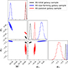 |
Fig. A.1. 1σ, 2σ, and 3σ likelihood contours of the GSMFs for our all-total, all-star-forming, and all-passive galaxy sample, as indicated in the legend. For each distribution, 104 random samples were generated. |
Appendix B: Robustness of the GSMF fits to the star-forming/passive classification
In this appendix, we investigate the extent to which our results depend on the specific division between star-forming and passive galaxies, that is, how robust our best-fit double Schechter parameters are against small changes in the dividing line used to separate the two populations in Sect. 4.1. To address this, we perform the following experiment. We first identify the 1σ confidence region based on the posterior distribution of the slope and intercept defining our fiducial dividing line in the log M − log SFR plane. From this region, we randomly extract 100 different (slope, intercept) pairs. Each of these defines a slightly different separation between star-forming and passive galaxies. For each resulting star-forming subsample, we compute the corresponding GSMF and perform a double Schechter fit. This procedure allows us to estimate the sensitivity of the fitted parameters to small variations in the classification between the two populations. We find that the resulting uncertainty on log M★ is ∼0.02, i.e. of the same order of magnitude as the random error obtained using our fiducial dividing line (cf. Table 2), while the errors on α1 and α2 are subdominant in comparison (0.03 and 0.01, respectively). This test, performed on the star-forming population, suggests that our results are not significantly affected by small perturbations in the classification.
All Tables
Best-fit double Schechter function parameters of the GSMFs of all, grouped, ungrouped, central, and satellite galaxies for different subsamples, as indicated.
Best-fit double Schechter function parameters of the GSMFs of grouped galaxies for different subsamples, as indicated.
Best-fit double Schechter function parameters of the GSMFs of star-forming and passive galaxies, corresponding to blue and red populations in other studies, as indicated.
Best-fit double Schechter function parameters of the GSMFs of central and satellite galaxies for different works, as indicated.
All Figures
|
Fig. 1. Distribution of the LP parameter. The dashed red line marks our lower limit (LP = −50) that has been applied to exclude galaxies with poor SED fits, caused by unreliable photometric data. |
| In the text | |
|
Fig. 2. Selection of star-forming and passive galaxies using the log M − log SFR plane. The dashed blue and red lines display the star-forming and passive population fits, respectively, whereas the solid green line displays our final dividing line. Star-forming galaxies are shown in cyan and passive galaxies in pink. Black dots refer to the 242 sources with LP < −50 (Sect. 3.1). |
| In the text | |
|
Fig. 3. GSMFs for our total, star-forming and passive galaxy populations, as indicated in the legend. Panel (a) full sample. Panels (b) and (c) grouped and ungrouped galaxies, respectively. In each sub-figure, the lower panel shows the GSMFs and the upper panel displays the raw number of galaxies as a function of stellar mass in each sample, as indicated. Dashed lines in panel (a) show the two individual Schechter components of each GSMF. |
| In the text | |
|
Fig. 4. Best-fit double Schechter function parameters of the GSMFs shown in Fig. 3, using the same colour-coding. The x-axes distinguish between all, grouped, and ungrouped galaxies; within each sample, the three ticks correspond to the total (T), star-forming (SF), and passive (P) subsamples. Corresponding corner plots illustrating the correlations among fitted parameters are provided in Figs. A.1–A.3. |
| In the text | |
|
Fig. 5. GSMFs for our total, central, satellite, and ungrouped galaxy populations, as indicated in the legend. Left: GSMFs for each entire population. Right: Subdivision into star-forming and passive galaxies. In each sub-figure, the lower panel shows the GSMFs and the upper panel displays the raw number of galaxies as a function of stellar mass in each sample, as indicated. |
| In the text | |
|
Fig. 6. Best-fit double Schechter function parameters of the GSMFs shown in Fig. 5, using the same colour-coding. The x-axes distinguish between central, satellite, and ungrouped galaxies; within each sample, the three ticks correspond to the total (T), star-forming (SF), and passive (P) subsamples. The black, blue and red horizontal bands show the results for the full parent, all-star-forming and all-passive samples, respectively, taken from Fig. 4. These reference lines are meant to be compared only with the T, SF, and P values in each subsample, respectively. Corresponding corner plots illustrating the correlations among fitted parameters are provided in Figs. A.4 and A.5. |
| In the text | |
|
Fig. 7. GSMFs of our grouped galaxy subsample colour-coded by Mhalo, as indicated in the legend. Panel a GSMFs as a function of Mdyn. Panels b and c further distinguish between passive and star-forming galaxies, and between central and satellite galaxies, respectively. In each sub-figure, the lower panel shows the GSMFs and the upper panel displays the raw number of galaxies as a function of stellar mass in each sample, as indicated. |
| In the text | |
|
Fig. 8. Best-fit double Schechter function parameters of the GSMFs shown in Fig. 7, using the same colour-coding by Mhalo. Panel a is in the centre, while panels b and c are on the left and right, respectively. For clarity, the vertical error bars corresponding to the passive galaxies in the left-hand panel and the centrals in the right-hand panel have been slightly offset to the right. Corresponding corner plots illustrating the correlations among fitted parameters are provided in Figs. A.6–A.8. |
| In the text | |
|
Fig. 9. Comparison between our best-fit double Schechter function parameters and literature values for different subsamples, as indicated in the legend. The likelihood contours show the 1σ, 2σ, and 3σ confidence regions for our fits. For each distribution, 104 random samples were generated. Symbols indicate the best-fit values from previous studies: circles for Peng et al. (2010) and squares for Weigel et al. (2016). |
| In the text | |
|
Fig. 10. Distribution of the LRT statistic obtained from 100 star-forming subsamples. The red dashed line marks our observed LRT value, which lies near the peak of the simulated distribution. This compatibility suggests that the data are consistent with the double Schechter model representing the true distribution, whereas the single Schechter function fails to provide an accurate description. |
| In the text | |
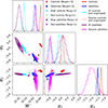 |
Fig. 11. Same as Fig. 9, but for different subsamples as indicated in the legend. |
| In the text | |
|
Fig. A.1. 1σ, 2σ, and 3σ likelihood contours of the GSMFs for our all-total, all-star-forming, and all-passive galaxy sample, as indicated in the legend. For each distribution, 104 random samples were generated. |
| In the text | |
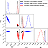 |
Fig. A.2. Same as Fig. A.1, but for the subsamples indicated. |
| In the text | |
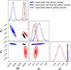 |
Fig. A.3. Same as Fig. A.1, but for the subsamples indicated. |
| In the text | |
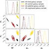 |
Fig. A.4. Same as Fig. A.1, but for the subsamples indicated. |
| In the text | |
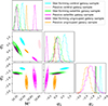 |
Fig. A.5. Same as Fig. A.1, but for the subsamples indicated. |
| In the text | |
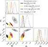 |
Fig. A.6. Same as Fig. A.1, but for the subsamples indicated. |
| In the text | |
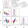 |
Fig. A.7. Same as Fig. A.1, but for the subsamples indicated. |
| In the text | |
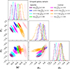 |
Fig. A.8. Same as Fig. A.1, but for the subsamples indicated. |
| In the text | |
Current usage metrics show cumulative count of Article Views (full-text article views including HTML views, PDF and ePub downloads, according to the available data) and Abstracts Views on Vision4Press platform.
Data correspond to usage on the plateform after 2015. The current usage metrics is available 48-96 hours after online publication and is updated daily on week days.
Initial download of the metrics may take a while.